Abstract

In the framework of precision experiments, the search for electric dipole moments and the precise determination of magnetic dipole moments (g-2) have since long been of prime interest. Hadronic decays offer the best accuracy, since only the kinematic information carried by a single neutrino per decay is lost. Thus, they reveal more easily precious information on the helicity of the initial tau lepton. However, in contrast to one- or two-body hadronic final states, the description of hadronic multi-body final states depends on the model for the hadronic current. In this work, we determine how the choice of a hadronic model impacts the extraction of tau electric and magnetic dipole moments.

1 Introduction

In light of the recent result on the anomalous magnetic moment of the muon $(g-2)_{\mu}$ [1], the study of the magnetic moments $\mu_{\tau}$ of the tau lepton receives new attention motivated by the mass of the tau lepton being about 17 times larger than the mass of the muon. In addition, electric dipole moments like $d_{\tau}$ are a key observable to search for effects of new physics, as well.

Both $\mu_{\tau}$ and $d_{\tau}$ may be studied measuring to high precision the production and subsequent decays of $\tau^{\pm}$-pairs in $e^{+}$-$e^{-}$-collisions at $B$-factories. Since the tau lepton has many different decay modes with none of them being dominant, the inclusion of the largest number of decay channels is required to statistically improve the precision of such measurements.

For most of the dominating decay modes like $(\pi\nu)$ or $(\ell\nu_{\ell}\nu_{\tau})$, we can construct the decay amplitudes from first principles. However, the amplitudes for hadronic multi-body final states depend on modelling the hadronic systems. Hadronic decays are particularly suited since they include only a single escaping neutrino in contrast to leptonic decays with two neutrinos ($\nu_{\tau}$ and $\nu_{\ell}$) missing in the final state. The latter results in large uncertainties in the reconstruction of the total event kinematics. The inclusion of hadronic decays (37% branching fraction), however, requires their very good understanding in order to reduce systematic uncertainties connected to their modelling. This is particularly true for hadronic multi-body ($n>2$) decays, which make up about $40\%$ of all hadronic decays [2]. Since for the measurement of the electric and magnetic moments the full $\tau^{\pm}$-pair event is studied, the inclusion of multi-body final states improves the exploitation of available data sets, presently mostly constrained to final states of $(e^{\pm}\nu_{e}\nu_{\tau})$, $(\mu^{\pm}\nu_{\mu}\nu_{\tau})$, $(\pi^{\pm}\nu_{\tau})$ and $(\rho^{\pm}\nu_{\tau})$, commonly used for such measurements [3].

The choice of the model for hadronic multi-body final states is not unique and we must thus estimate the impact of the differences between the true model and the analysis model on the measurement of the tauon electric and magnetic moments.

This article is structured as follows: in Sec. 2 we introduce the form factors $F_{2}$ and $F_{3}$ and construct the spin-density matrix for the production of $\tau^{\pm}$-pairs. In Sec. 3, we elaborate on the effects of the escaping neutrinos on the determination of $F_{2/3}$. In Sec. 4, we introduce the hadronic model required for hadronic multi-body final states. In Sec. 5, we construct so-called optimal observables used to extract the value of $F_{2/3}$ from data and use them to study the impact of the hadronic model on the measurement of $F_{2/3}$, as described in Sec. 6 using simulated data.

2 Form factors

The coupling of $\tau^{\pm}$-pairs to the photon field is described by:

$$-e\bar{u}_{\lambda_{-}}\Gamma^{\mu}v_{\lambda_{+}},$$ (1)

where $u_{\lambda^{-}}$ and $v_{\lambda^{+}}$ are the usual Dirac-spinors of the tauons with helicities $\lambda_{\pm}$ and the $\Gamma^{\mu}$ is given by:

$$\Gamma^{\mu}=F_{1}(q^{2})\gamma^{\mu}+\frac{iF_{2}(q^{2})}{2m_{\tau}}\sigma^{\mu\nu}q_{\nu}+\frac{F_{3}(q^{2})}{2m_{\tau}}\sigma^{\mu\nu}\gamma^{5}q_{\nu},$$ (2)

where $q^{\mu}$ is the total four-momentum. $F_{1}(q^{2})$ is the Dirac form-factor and $F_{2}(q^{2})$ is the Pauli form-factor. $F_{2/3}$ are connected to the electric and magnetic dipole moments via:

$$F_{2}(q^{2}=0)+1=\frac{2m_{\tau}}{eQ_{\tau}}\mu_{\tau}\quad\text{and}\quad F_{3}(q^{2}=0)=\frac{2m_{\tau}}{eQ_{\tau}}d_{\tau}.$$ (3)

The amplitude for the $\tau^{\pm}$-pair production in $e^{+}$-$e^{-}$-collisions is then given by:

$$\mathcal{A}_{\lambda_{e^{-}}\lambda_{e^{+}}\lambda_{-}\lambda_{+}}=\frac{e^{2}}{q^{2}}\cdot\bar{v}_{\lambda_{e^{p}}}\gamma_{\mu}u_{\lambda_{e^{-}}}\cdot u_{\lambda_{-}}\Gamma^{\mu}v_{\lambda_{+}},$$ (4)

where $\lambda_{e^{-}}$ and $\lambda_{e^{+}}$ are the helicities of the beam particles. From this amplitude, we can construct the spin-density-matrix for the $\tau^{\pm}$-pair, which for the case of unpolarized $e^{+}$ and $e^{-}$ beams is given by:

$$\chi_{\lambda_{-}\lambda_{+}\lambda_{-}^{\prime}\lambda_{+}^{\prime}}=\frac{1}{4}\sum_{\lambda_{e^{\pm}}}\mathcal{A}_{\lambda_{e^{-}}\lambda_{e^{+}}\lambda_{-}\lambda_{+}}^{*}\mathcal{A}_{\lambda_{e^{-}}\lambda_{e^{+}}\lambda_{-}^{\prime}\lambda_{+}^{\prime}}.$$ (5)

Non-zero values of the form factors $F_{2/3}$ change the spin-density matrix and thus the spin-correlations of the produced $\tau^{\pm}$-pair. The changes to the spin-density matrix elements related to $\Re/\Im(F_{2/3})$ are shown as function of the $\cos(\theta)$ in Fig. 1, where $\theta$ is the production angle of the $\tau^{-}$ with respect to the incoming electron. The varying symmetry properties of the spin density matrix elements can be seen, and only $\Re(F_{2})$ changes the total production cross-section. For most form factors and spin combinations, extreme forward and backward angles as well as 90 degrees provide no sensitivity. Here, production angles around $\pm 45$ degrees seem most important.

Since tauons decay before crossing any detector element, spin-correlations of the $\tau^{\pm}$-pair can only be accessed through the angular distributions of the $\tau^{\pm}$ decay products. In this work, we focus on such spin correlations in $\tau^{\pm}$-pair production and the corresponding intensity distribution $\mathcal{I}$ of the decay products of both $\tau^{\pm}$ is constructed via:

$$\mathcal{I}=\sum_{\lambda^{(\prime)}_{\pm}}\chi_{\lambda_{-}\lambda_{+}\lambda_{-}^{\prime}\lambda_{+}^{\prime}}\cdot D^{-}_{\lambda_{-}\lambda_{-}^{\prime}}\cdot D^{+}_{\lambda_{+}\lambda_{+}^{\prime}},$$ (6)

where $D^{\pm}_{\lambda_{\pm}\lambda_{pm}^{\prime}}$ are the spin-density matrices for the $\tau^{\pm}$ decays.

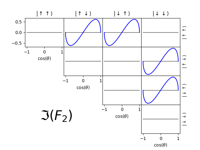
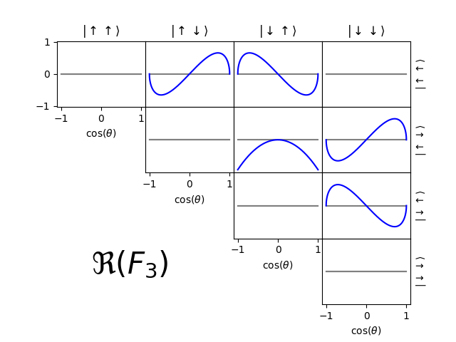
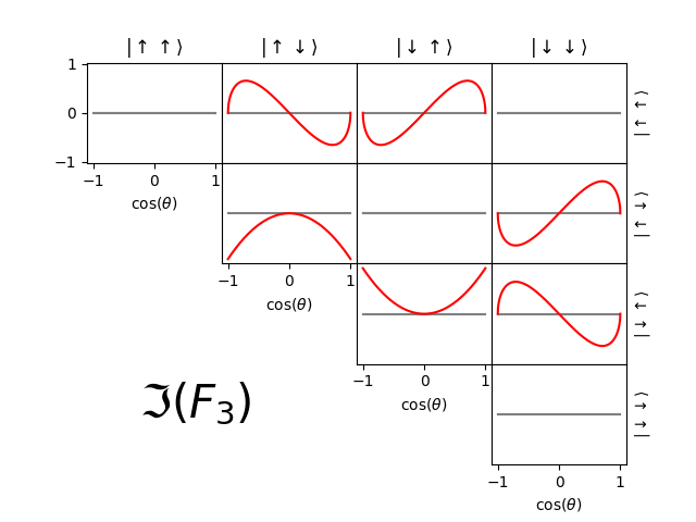
Figure 1: Contributions from the form-factors $F_{2/3}$ to the $\tau^{\pm}$-pair production spin-density matrix as function of the production angle $\cos(\theta)$. Contributions from the real and imaginary parts of $F_{2/3}$ are on the left and right, respectively. The influence of $F_{2}$ and $F_{3}$ are shown on the top and bottom row. Real and imaginary parts of the spin-density matrix are shown as red and blue lines, respectively. The vertical axis range is the same for all 10 plots of one contribution and is indicated on the leftmost sub-plot. Entries below the diagonal are omitted, since they are hermitian conjugates of the upper-diagonal entries.

3 Effects of neutrino kinematics

In principle, all decay modes of the $\tau$-lepton are suitable for the determination of the form factors $F_{2/3}$. Simple accuracy studies similar to studies presented in Sec. 6 show that the accuracy for the form-factors $F_{2/3}$ is similar for all combinations of the dominant $\tau^{\pm}$ decay modes. This, however, requires the final-state kinematic information to be complete, and thus the intensity distribution $\mathcal{I}$ given in Eq. (6) can simply be calculated.

However, since in every decay at least one neutrino is escaping, calculating the intensity distribution is no longer possible and unmeasurable degrees of freedom have to be integrated out. In events, where only a single neutrino escapes in each tau decay—making two in total—a two-fold kinematic ambiguity arises for the direction of the tauons that has to be averaged in the calculation of $\mathcal{I}$. For this, both $\tau^{-}$ and $\tau^{+}$ must decay hadronically. For every $\tau^{\pm}$ decaying leptonically, an additional integration has to be performed:

$$\mathcal{I}\to\iiint\mathcal{I}\,\mathrm{d}\phi\,\mathrm{d}\!\cos\theta\,\mathrm{d}m_{\nu\bar{\nu}}^{2},$$ (7)

where $m_{\nu\bar{\nu}}$ is the invariant mass of the escaping $(\nu\bar{\nu})$-system and $\theta$ and $\phi$ the polar and azimuthal angle of the $\tau$ neutrino within this system.

This loss of kinematic information decreases the accuracy for the form factors $F_{2/3}$ depending on the particular combination of decay channels used. This reduction in accuracy is summarized in Table 1, comparing the accuracies $\delta$ obtained with integrated and with fully known kinematic information:

$$x_{\delta\Re/\Im(F_{2/3})}=\frac{\delta_{\text{integrated}}\Re/\Im(F_{2/3})}{\delta_{\text{known}}\Re/\Im(F_{2/3})}.$$ (8)

The averaging of the two-fold ambiguity for hadronic decays thus leads to a small decrease in accuracy, while the integration given in Eq. (7) for leptonic decays has a much larger effect, in particular for $\Re(F_{3})$.

Thus, an increase of the usable data set of hadronic decays would improve the accuracies for $F_{2/3}$. In this work, we discuss the inclusion of the multi-body final-state with the highest branching fraction of $9.31\%$[2]: $\tau^{\pm}\to\pi^{\mp}\pi^{\pm}\pi^{\pm}+\nu$. Since this decay mode can be combined with all available decay modes of the opposite-sign $\tau$, its inclusion would increase the number of available purely hadronic events by a factor 1.57.

Table 1: Decrease of accuracy due to the loss of kinematic information due to escaping neutrino kinematics for 16 combinations of $\tau^{\pm}$ decay modes. The numbers are based on sets of $10^{6}$ simulated events.

$\tau^{-}$ mode	$\tau^{+}$ mode	$x_{\delta\Re(F_{2})}$	$x_{\delta\Im(F_{2})}$	$x_{\delta\Re(F_{3})}$	$x_{\delta\Im(F_{3})}$
$\pi^{-}\nu_{\tau}$	$\pi^{+}\bar{\nu}_{\tau}$	$1.09$	$1.60$	$1.61$	$1.06$
$\pi^{-}\nu_{\tau}$	$\rho^{+}\bar{\nu}_{\tau}$	$1.11$	$1.19$	$1.19$	$1.10$
$\pi^{-}\nu_{\tau}$	$\mathrm{e}^{+}\bar{\nu}_{\tau}\nu_{\mathrm{e}}$	$2.07$	$1.75$	$3.84$	$1.92$
$\pi^{-}\nu_{\tau}$	$\mu^{+}\bar{\nu}_{\tau}\nu_{\mu}$	$2.06$	$1.72$	$3.73$	$1.92$
$\rho^{-}\nu_{\tau}$	$\pi^{+}\bar{\nu}_{\tau}$	$1.11$	$1.19$	$1.19$	$1.10$
$\rho^{-}\nu_{\tau}$	$\rho^{+}\bar{\nu}_{\tau}$	$1.11$	$1.26$	$1.15$	$1.10$
$\rho^{-}\nu_{\tau}$	$\mathrm{e}^{+}\bar{\nu}_{\tau}\nu_{\mathrm{e}}$	$2.03$	$1.79$	$3.18$	$1.92$
$\rho^{-}\nu_{\tau}$	$\mu^{+}\bar{\nu}_{\tau}\nu_{\mu}$	$2.04$	$1.79$	$3.17$	$1.92$
$\mathrm{e}^{-}\nu_{\tau}\bar{\nu}_{\mathrm{e}}$	$\pi^{+}\bar{\nu}_{\tau}$	$2.09$	$1.81$	$3.97$	$2.04$
$\mathrm{e}^{-}\nu_{\tau}\bar{\nu}_{\mathrm{e}}$	$\rho^{+}\bar{\nu}_{\tau}$	$2.03$	$1.75$	$3.32$	$1.82$
$\mathrm{e}^{-}\nu_{\tau}\bar{\nu}_{\mathrm{e}}$	$\mathrm{e}^{+}\bar{\nu}_{\tau}\nu_{\mathrm{e}}$	$3.45$	$2.28$	$21.83$	$3.33$
$\mathrm{e}^{-}\nu_{\tau}\bar{\nu}_{\mathrm{e}}$	$\mu^{+}\bar{\nu}_{\tau}\nu_{\mu}$	$3.73$	$2.28$	$11.72$	$3.29$
$\mu^{-}\nu_{\tau}\bar{\nu}_{\mu}$	$\pi^{+}\bar{\nu}_{\tau}$	$2.07$	$1.79$	$3.92$	$2.02$
$\mu^{-}\nu_{\tau}\bar{\nu}_{\mu}$	$\rho^{+}\bar{\nu}_{\tau}$	$2.03$	$1.72$	$3.25$	$1.83$
$\mu^{-}\nu_{\tau}\bar{\nu}_{\mu}$	$\mathrm{e}^{+}\bar{\nu}_{\tau}\nu_{\mathrm{e}}$	$5.83$	$2.28$	$12.26$	$3.31$
$\mu^{-}\nu_{\tau}\bar{\nu}_{\mu}$	$\mu^{+}\bar{\nu}_{\tau}\nu_{\mu}$	$3.11$	$2.32$	$14.41$	$3.27$

4 Hadronic current model for tau decays

The spin-density matrices $D^{\pm}_{\lambda_{\pm}\lambda_{\pm}^{\prime}}$ used in Eq. (6) for the decays of the $\tau^{\pm}$ are constructed via:

$$D^{\pm}_{\lambda_{\pm}\lambda_{\pm}^{\prime}}=\mathfrak{A}_{\lambda_{\pm}}^{\pm*}\mathfrak{A}_{\lambda_{\pm}^{\prime}}^{\pm},$$ (9)

where $\mathfrak{A}_{\lambda_{\pm}}^{\pm}$ is the amplitude for the decay of a $\tau^{\pm}$ with helicity $\lambda^{\pm}$ into a particular final-state. For $\tau^{-}$ decays into hadronic final-states, this amplitude is given by:

$$\mathfrak{A}_{\lambda_{-}}^{-}\propto\bar{u}_{\nu}\gamma_{\mu}(1-\gamma^{5})u_{\lambda_{-}}\,J_{\text{had}}^{\mu}=\ell_{\lambda_{-}\mu}J_{\text{had}}^{\mu},$$ (10)

where $J_{\text{had}}^{\mu}$ is the hadronic current describing the hadronic dynamics of the decay. For decays into a single $\pi^{-}$ or $\rho^{-}$ and an escaping $\nu_{\tau}$, the corresponding hadronic currents are given by:

$$J_{\pi^{-}}^{\mu}\propto p_{\pi}^{\mu}\quad\text{and}\quad J_{\rho^{-}}^{\mu}\propto\text{BW}_{\rho}(p_{\rho}^{2})\left(\eta^{\mu}_{\nu}-\frac{p_{\rho}^{\mu}p_{\rho\nu}}{p_{\rho}^{2}}\right)\left(p_{\pi^{-}}^{\nu}-p_{\pi^{0}}^{\nu}\right).$$ (11)

$\text{BW}_{\rho}(s)$ describes the dynamic amplitude of the intermediate $\rho(770)$ resonance, subsequently decaying into two pions. Since this only acts as a scalar factor in the hadronic current, it cancels in the construction of the optimal observables defined in Eq. (14) and thus does not affect the measurement of $F_{2/3}$.

The formulation of the hadronic current in terms of final-state particle momenta for multi-body final-states is not straightforward and requires modelling of the hadron dynamics. In this work, we study the decay $\tau^{-}\to 3\pi^{\pm}+\nu_{\tau}$ and model the hadronic current within the isobar model, following previous analyses [4] and [6]. In the isobar model, the total hadronic current is composed of several partial waves, which each corresponds to a particular set of quantum numbers $J^{PC}$ for the three-pion system, which subsequently decays into a $\pi^{-}$ and another known resonance finally decaying into $\pi^{+}+\pi^{-}$, hereafter called the isobar.

$$J_{3\pi}^{\mu}=\sum_{w\in\{\text{waves}\}}c_{w}j_{w}^{\mu}.$$ (12)

The complex-valued coefficients $c_{w}$ encode the strengths and relative phases of the individual partial waves, while the partial-wave currents $j_{w}^{\mu}$ encode their specific dependence on the final-state four-momenta. A detailed formulation of the $j_{w}^{\mu}$ can be found in Ref. [6]. Besides the isobar model presented here, there are other models for $J_{3\pi}^{\mu}$, e.g. R$\chi$T models [7] also commonly used.

5 Optimal observables

The tau lepton form factors $F_{2/3}(q^{2})$, which contain the here sought after physics observables $\mu_{\tau}$ and $d_{\tau}$ only enter in the description of the spin density matrix for the $\tau^{\pm}$ pair production [see eq. (5)]. We may thus single out their effect on the intensity $\mathcal{I}$ by rewriting equation 6:

$$\mathcal{I}=\mathcal{I}_{\text{SM}}+\sum_{x\in\{\Re/\Im(F_{2/3})\}}x\cdot\mathcal{I}_{x},$$ (13)

where $\mathcal{I}_{\text{SM}}$ is the standard model intensity distribution and $\mathcal{I}_{x}$ are the specific intensity distributions corresponding the non-zero real and imaginary parts $\Re/\Im(F_{2/3})$. Since the form factors $F_{2/3}$ are known to be small, quadratic terms in the form factors are neglected.

Each observable (form factors and thus the dipole moments) depends on specific relations among the measurable quantities of the final state particles. Using this expansion, we can define four optimal observables $OO_{x}$, one for each of the four $x\in\{\Re/\Im(F_{2/3})\}$, being optimally sensitive to the form factors [8]:

$$OO_{x}=\frac{\mathcal{I}_{x}}{\mathcal{I}_{\text{SM}}}.$$ (14)

Using these observables, the form factors can be extracted via the expectation values of the corresponding $OO_{x}$ obtained for a given data-set:

$$\left\langle OO_{x}\right\rangle=a_{x}\cdot x+b_{x},$$ (15)

where the coefficients $a_{x}$ and $b_{x}$ are determined from simulations.

6 Studies using simulated data

We now study the impact of the hadronic model on the determination of $F_{2/3}$ using the optimal observables defined in Sec. 5. For this we construct a hadronic toy model consisting of the following nine partial waves:

$$\begin{array}[]{ccc}a_{1}[\rho\pi]_{S}&a_{1}[\rho\pi]_{D}&a_{1}[f_{2}\pi]_{P}\\ a_{1}[\sigma\pi]_{P}&a_{1}[f_{0}\pi]_{P}&\pi_{1}[\rho\pi]_{P}\\ \pi[\sigma\pi]_{S}&\pi[f_{0}\pi]_{S}&\pi[\rho\pi]_{P}\end{array}$$ (16)

where the naming scheme $X[\xi\pi]_{L}$ denotes a three-pion resonance $X$ (the hadronic system) decaying into an isobar $\xi$ and a pion with relative orbital angular momentum $L$. The subsequent decay of the isobar $\xi$ into two pions is implied and in turn described by a set of known decay amplitudes. Each resonance $X$ represents a set of quantum numbers $J^{PC}$.

For the model, we used partial-wave coefficients $c_{w}$ loosely inspired by a partial-wave analysis of the three-pion final state in Ref. [9]. The dominant wave in this model is the $a_{1}[\rho\pi]_{S}$ wave, as is expected following previous analyses [4]. Using our toy model, we generated data sets with $10^{6}$ $\tau^{\pm}$-pair events, where the $\tau^{-}$ decays into $(3\pi^{\pm}+\nu_{\tau})$ according to the model described above, while the $\tau^{+}$ decays into $(\pi^{+}+\bar{\nu}_{\tau})$. In total, we generated four toy data sets, where one of each of the four $\Re/\Im(F_{2/3})$ takes the value of 0.01, while the other three values remain 0.

In a first study, we analyze the pseudo data using the same hadronic model as used for the simulation and extract the form-factors. We found no bias and an accuracy comparable to the other hadronic decay modes $(\pi^{-}+\nu_{\tau})$ and $(\rho^{-}+\nu_{\tau})$ for the same number of events is obtained. For $10^{6}$ simulated events, we find:

$$\begin{array}[]{ll}\delta\Re(F_{2})=0.0006;&\delta\Im(F_{2})=0.0007;\\ \delta\Re(F_{3})=0.0009;&\delta\Im(F_{3})=0.0005,\end{array}$$ (17)

In a second study, we analyzed the same simulated data sets but now using a simplified model for the hadronic current, namely now only comprising the $a_{1}[\rho\pi]_{S}$ wave. To quantify the similarity of two hadroic models, we define the model overlap $\omega_{m,m^{\prime}}$ of two models $m$ and $m^{\prime}$ for the hadronic current as the normalized product of the total hadronic currents $J^{\mu}_{m}$, contracted with the corresponding leptonic current $\ell_{\lambda_{-}}^{\mu}$ and integrated over the full Lorentz invariant phase space (LIPS)::

$$\omega_{m,m^{\prime}}=\left|\int\mathrm{dLIPS}\,\left(J_{m}^{\mu}\ell_{\lambda_{-}\mu}\right)^{*}\left(\ell_{\lambda_{-}\nu}J_{m^{\prime}}^{\nu}\right)\right|\Bigg{/}\Big{(}\mathcal{N}_{m}\cdot\mathcal{N}_{m^{\prime}}\Big{)},$$ (18)

with the leptonic current $\ell_{\lambda_{-}}^{\mu}$ defined in Eq. (10). The model-overlap of $\omega_{\text{true},\text{ana}}$ of the simplified model with the model used for simulation was $78\%$.

For this study, we also re-determined the coefficients $a_{x}$ and $b_{x}$ defined in Eq. (15) so that they correspond to our simplified analysis model. Repeating our analysis with a wrong hadronic model results in the following values for $\Re/\Im(F_{2/3})$:

$$\begin{array}[]{ll}\Re(F_{2})=0.0529\pm 0.0008;&\Im(F_{2})=0.0118\pm 0.0008;\\ \Re(F_{3})=0.0086\pm 0.0012;&\Im(F_{3})=0.0079\pm 0.0005,\end{array}$$ (19)

while the true value for these quantities is always 0.01. We find, that $\Re(F_{2})$ is largely over-estimated, while the effect in $\Im(F_{2})$ is not very large. $\Re(F_{3})$ and $\Im(F_{3})$ suffer an under-estimation, which, however, is less than for $\Re(F_{2})$. If the true value is set to $0$, the bias in $\Re(F_{2})$ persists, while we observe no bias for $\Re/\Im(F_{3})$ in this case.

We now repeated this procedure with different de-tuned analysis models for every individual partial wave given in Eq. (16). For this, we scale up one individual partial wave coefficient $c_{w}$ [see Eq. (12)] from the true model such, that the model overlap $\omega_{\text{true},\text{ana}}$ drops to $95\%$, while keeping the remaining coefficients at their nominal values. Doing so, we find that the values obtained for $F_{3}$ and $\Im(F_{2})$ are consistent with the input values, regardless of the wave scaled. Thus, the extraction of these three quantities appears to be rather robust with respect to changes in the hadronic model.

In the case of $\Re(F_{2})$, we observe a significant bias due to the mismatch between generator and analysis hadronic model. This bias depends on the individual partial wave that is scaled in the particular study and is given in Tab. 2.

Table 2: $\Re(F_{2})$ extracted from a simulated data set with an input value of $\Re(F_{2})=0.01$, analyzed with a single de-tuned partial wave. The statistical uncertainties of all values shown are $0.0007$.

De-tuned wave	$a_{1}[\rho\pi]_{S}$	$a_{1}[\rho\pi]_{D}$	$a_{1}[f_{2}\pi]_{P}$	$a_{1}[\sigma\pi]_{P}$	$a_{1}[f_{0}\pi]_{P}$
$\Re(F_{2})$	0.0178	0.0168	0.0144	0.0169	0.0143
De-tuned partial wave	$\pi_{1}[\rho\pi]_{P}$	$\pi[\sigma\pi]_{S}$	$\pi[f_{0}\pi]_{S}$	$\pi[\rho\pi]_{P}$
$\Re(F_{2})$	0.0147	0.0186	0.0162	0.0180

In a final study, we de-tuned the $a_{1}[\rho\pi]_{S}$-wave such that the model-overlap $\omega_{\text{true},\text{ana}}=99\%$. In this case, we obtain:

$$\begin{array}[]{ll}\Re(F_{2})=0.0112\pm 0.0007;&\Im(F_{2})=0.0102\pm 0.0007;\\ \Re(F_{3})=0.0097\pm 0.0009;&\Im(F_{3})=0.0103\pm 0.0005.\end{array}$$ (20)

Thus, we find that a proper model for the hadronic current $J_{3\pi}^{\mu}$ alleviates possible bias in the determination of $\Im(F_{2})$ and $F_{3}$, while the bias in $\Re(F_{2})$ remains significantly larger than the uncertainty, even for a model overlap very close to unity. Since $\Re(F_{2})$ is the only quantity that alters the total cross-section (see Fig. 1), it might be advisable to neglect the spin-information of the decays and only use the total $\tau^{\pm}$-pair production cross-section. Doing so, we find for the same simulated data introduced above:

$$\Re(F_{2})=0.0108\pm 0.0015.$$ (21)

Even though the accuracy for $\Re(F_{2})$ is worse by a factor of two, this result is independent of a hadronic model and thus is not affected by model bias. Including only the spin-information from the $(\pi^{+}+\bar{\nu}_{\tau})$ decay does not improve the accuracy given in Eq. (21). This is expected, since $\Re(F_{2})$ only affects the correlation of both $\tau^{\pm}$ spins. However, the measurement of the total cross-section requires that all radiative corrections are known and is typically very difficult, since it introduces new sources of systematic uncertainties.

Evaluating the distributions from Fig. 1 for each partial wave, we could not single out particular waves being specifically more sensitive to the observation of EDM or MDMs than others. The scheme of optimized variables would, however, take into account such possible effects.

7 Conclusion

We studied the determination of the tauon form factors $F_{2}$ and $F_{3}$ using simulated $(3\pi^{\pm}+\nu_{\tau})$$\times$ $(\pi^{+}+\bar{\nu}_{\tau})$ $\tau^{\pm}$-events. We find the $3\pi^{\pm}$ hadronic final-state to give an accuracy on the form-factors comparable to other hadronic channels, assuming the model for the hadronic current $J_{3\pi}^{\mu}$ to be perfect. Thus, this decay channel will help to significantly increase usable data for purely hadronically decaying $\tau^{\pm}$-pair events. For a simulated data set of $10^{6}$ events, we obtain an accuracy for $\mu_{\tau}$ and $d_{\tau}$ of:

$$\begin{array}[]{ll}\delta\Re(\mu_{\tau})=3.46\times 10^{-18}e\text{cm}&\delta\Im(\mu_{\tau})=3.58\times 10^{-18}e\text{cm}\\ \delta\Re(d_{\tau})=4.66\times 10^{-18}e\text{cm}&\delta\Im(d_{\tau})=2.61\times 10^{-18}e\text{cm}.\end{array}$$ (22)

However, the model for $J_{3\pi}^{\mu}$ is not known a priori and all models currently used, e.g. the isobar model or R$\chi$T models [4, 6, 7], are based on assumptions, a perfect hadronic model is currently not available. Thus, we extended our study to hadronic models for $J^{\mu}_{3\pi}$ that differ from the true model and found a small bias in the extraction of $F_{3}$ and $\Im(F_{2})$, while $\Re(F_{2})$ is heavily over-estimated.

The observed bias results in an under-estimation of $\Re/\Im(F_{3})$, which in turn vanishes as the analysis model approached the true model. The bias in $\Re(F_{2})$, however, remains significant even at a model overlap $\omega_{\text{true},\text{ana}}=99\%$ and thus seems to prohibit the use of the $3\pi^{\pm}$ channel in a determination of $\Re(F_{2})$. However, since $\Re(F_{2})$ alters the total $\tau^{\pm}$ pair production cross-section, we may ignore spin effects for such final states and still determine $\Re(F_{2})$. Ignoring spin-correlations decreases the accuracy by a factor of two, but removes the strong model-dependence.

Finally, we stress that a good knowledge of the hadron dynamics of multi-particle $\tau^{\pm}$ decays is prerogative for their inclusion in precision measurements like $F_{2/3}(q^{2})$. A simple approximation of the hadronic current by the dominating $a_{1}\to[\rho\pi]_{S}$ contribution does not suffice, since according to current knowledge it only describes around $70\%$ of the $\tau\to 3\pi+\nu$ intensity [4].

References

- [1] B. Abi et al. [Muon g-2], Phys. Rev. Lett. 126 (2021) 141801, [arXiv:2104.03281].
- [2] P.A. Zyla et al. (Particle Data Group), Prog. Theor. Exp. Phys. 2020, 083C01 (2020) and 2021 update.
- [3] K. Inami et al. [Belle], Phys. Lett. B 551 (2003) 16–26, [arXiv:hep-ex/0210066].
- [4] D. M. Asner et al. [CLEO], Phys. Rev. D 61 (2000), 012002, [arXiv:hep-ex/9902022].
- [5] F. Krinner and N. Kaiser, [arXiv:2110.05358].
- [6] F. Krinner and S. Paul, EPJ C 81 (2021), 1073, [arXiv:2107.04295].
- [7] D. Gomez Dumm, A. Pich and J. Portoles, Phys. Rev. D 69 (2004), 073002, [arXiv:hep-ph/0312183].
- [8] D. Atwood and A. Soni, Phys. Rev. D 45, 2405-2413 (1992).
- [9] C. Adolph et al. [Compass], Phys. Rev. D 95 (2017) 032004, [arXiv:1509.00992].