Revisiting Neuron Coverage for DNN Testing: A Layer-Wise and Distribution-Aware Criterion1

Abstract

Various deep neural network (DNN) coverage criteria have been proposed to assess DNN test inputs and steer input mutations. The coverage is characterized via neurons having certain outputs, or the discrepancy between neuron outputs. Nevertheless, recent research indicates that neuron coverage criteria show little correlation with test suite quality.

In general, DNNs approximate distributions, by incorporating hierarchical layers, to make predictions for inputs. Thus, we champion to deduce DNN behaviors based on its approximated distributions from a layer perspective. A test suite should be assessed using its induced layer output distributions. Accordingly, to fully examine DNN behaviors, input mutation should be directed toward diversifying the approximated distributions.

This paper summarizes eight design requirements for DNN coverage criteria, taking into account distribution properties and practical concerns. We then propose a new criterion, NeuraL Coverage (NLC), that satisfies all design requirements. NLC treats a single DNN layer as the basic computational unit (rather than a single neuron) and captures four critical properties of neuron output distributions. Thus, NLC accurately describes how DNNs comprehend inputs via approximated distributions. We demonstrate that NLC is significantly correlated with the diversity of a test suite across a number of tasks (classification and generation) and data formats (image and text). Its capacity to discover DNN prediction errors is promising. Test input mutation guided by NLC results in a greater quality and diversity of exposed erroneous behaviors.

I Introduction

Recent work has incorporated software testing methodologies to successfully evaluate DNN [44, 51, 45]. However, fundamental understanding of a DNN’s mechanism has remained largely unexplored due to its intrinsic non-linearity. As a result, DNN evaluation is highly dependent on the test suite’s representativeness. Testing criteria are thus required to characterize a test suite’s quality and toward which the input mutations can comprehensively explore DNN behaviors.

Similar to how coverage criteria are developed in software testing, recent research proposes several neuron coverage criteria. In principle, the current criteria are mostly designed to monitor the outputs of neurons in a DNN model. They argue that each neuron is an “individual computing unit” (as the authors put it [33]), or “individually encoding a feature” [28], comparable to a statement in traditional software. Further, despite neuron outputs are continuous, existing criteria often first convert neuron outputs into discrete states (e.g., activated or not) to reduce the modeling complexity. Thus, by analyzing the discrete states of neurons, the DNN coverage exercised by an input is measured. Recent works measure the distance between neuron output traces of a new input and historical inputs to decide the discrepancy of the new input. The derived coverage is calculated via clusters [32] or discretized buckets over some distance scores [22, 23].

However, the key assumption — each neuron is an individual computing unit — often does not hold true for modern DNNs. Given a DNN is composed of stacked and non-linear layers, the intermediate outputs (also known as latent representations) from neurons are continuous and highly entangled. Disentangling intermediate outputs remains a long-lasting challenge [26, 35, 27]. Recent research also points out that the efficacy of a test suite to uncover faults and existing neuron coverage attained by the test suite are not always positively correlated [16].

Establishing proper DNN coverage criteria requires a principled understanding about how DNN performs computations, which is fundamentally different with traditional software. A DNN, as a composition of non-linear functions (i.e., layers), extracts task-oriented features (e.g., classification vs. localization) and then makes decisions. Features, that are hierarchically propagated by layer outputs, approximate the posterior distribution of underlying explanatory factors $H$ for an input $x$, namely $P(H|x)$ [4, 5]. For example, an image classifier generates a set of posterior distributions $P(h_{i}|x)$ (where $i$ is the layer index and $h_{i}\in H$) with each $h_{i}$ depicts class-invariant properties of an image from different aspects (e.g., shape, texture) [4]. In addition, the dependability of a DNN is defined as the degree to which the distribution, approximated on training data, is accurate when applied to real test data.

This work initializes a principled view on designing DNN coverage criteria, by assessing test inputs regarding their induced layer output distributions. We first concretize our focus into eight design requirements. These requirements characterize the distribution approximated by a DNN from various aspects, and also take practical constraints (e.g., cost, hyper-parameter free) into account. Then, we propose a new coverage criterion, namely NLC (NeuraL Coverage), that can fully meet the design requirements. NLC is referred to as “neural coverage” rather than neuron coverage since we focus on the overall activity of groups of neurons (i.e., each layer) and consider relations of neurons (different with all existing criteria; see comparison in Sec. III-B). Our evaluation includes nine DNNs that analyze various data formats (e.g., image, text) and perform various tasks (e.g., classification, generation). We show that NLC is substantially correlated with the diversity and capacity of a test suite to reveal DNN defects. Meanwhile, by taking NLC as the fuzzing feedback, we show that more and diverse errors can be found, and the mutations guided by NLC generate more natural inputs. Our contributions are summarized as:

• This work advocates to design DNN testing criteria via a principled understanding about how DNN, with its hierarchical layers, approximate distributions. We argue that a proper DNN testing criterion should model the continuous neuron outputs and neuron entanglement, instead of analyzing each neuron individually.

• We propose eight design requirements by considering the distributions approximated by a DNN and practical implementation considerations. We accordingly design NLC, satisfying all these requirements.

• We show that NLC can better assess the quality of test suites. NLC is particularly correlated with the diversity and fault-revealing capacity of a test suite. Fuzz testing under the guidance of NLC can also detect a large number of errors, which are shown as diverse and natural-looking.

Artifact: We released our artifact and supplementary materials at https://github.com/Yuanyuan-Yuan/NeuraL-Coverage [1].

II Preliminary and Overview

DNNs are often explained from the distribution approximation perspective [4, 5, 40]. Following, this section provides a high-level overview of DNNs to motivate NLC.

“Neural” and “Network”. The term neural in DNN may be obscure. In cognitive science, neural signifies non-linear functions (e.g., Sigmoid) in DNNs that simulate how human neurons process signals [37, 6]. DNNs are powerful at analyzing high-dimensional media data due to their non-linearity [3, 4]. Neurons in a layer are therefore highly entangled, impeding to comprehend the DNN’s internal mechanics. Moreover, outputs of neurons are continuous. The term network in DNN refers to topological connections of non-linear layers. Each layer has a group of neurons cooperating to process certain input features. The DNN hierarchy is established by gradually abstracting features from shallow to deep layers. For instance, image classifiers commonly collect shapes in an image at shallow layers and texture at deeper layers [14, 50]. Each layer (not each neuron) serves a minimal computing unit, whose output distribution encodes its focused features.

Given a collection of data $X$ labeled as $Y$, most popular DNNs can be categorized as discriminative and generative models, depending on how $X$ and $Y$ are involved in the distribution approximation.

Discriminative Models. Deep discriminative models approximate the conditional probability distribution $P(Y|X)$. A classification model requires $Y$ as discrete labels, and a regression model (e.g., forecasting) requires $Y$ as a range of continuous values. For instance, a convolutional neural network (CNN) can classify images by extracting features (conveyed via outputs of intermediate neurons) and making decisions in one forward propagation. A layer outputs a conditional distribution denoting the extracted input features at this layer [4, 5, 40]. And with the extracted features getting more abstract at deeper layers, the ending layer returns the probability that the input belongs to each label. Sequential data, such as text, is processed by recurrent models (e.g., LSTM) in a similar way.

Generative Models. Another popular paradigm is the deep generative model, which estimates the joint probability distribution $P(X,Y)$ of data $X$ and label $Y$. The most common models are VAE [24] and GAN [15]. Generative models are primarily adopted to synthesize realistic data. To do so, both VAE and GAN project the data distribution to a simple distribution (e.g., normal distribution). To generate realistic outputs, random inputs sampled from the pre-defined distribution are fed into deep generative models.

Visualizing DNN Outputs. We empirically assess and visualize the distribution of intermediate neurons’ outputs. We prepare a DNN (denoted as Net; see implementation in [1]) with two neurons $n_{1}$ and $n_{2}$ (thus the dimensions are two) in the last layer and extend Net into 1) a VAE, 2) a class-conditional VAE (C-VAE), and 3) a classifier. The three models are trained on the MNIST dataset [12] for 1) random image generation, 2) labeled image (e.g., “2”) generation, and 3) image classification. In short, these models inherit the same structure from Net yet perform different tasks by using different trailing layers.

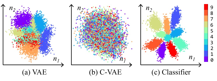
Figure 1: Visualization of $n_{1}$ and $n_{2}$’s outputs in three models extended from Net. X- and y-axis are outputs of $n_{1}$ and $n_{2}$.

Fig. 1 shows the outputs of $n_{1}$ and $n_{2}$ in these models. Each dot denotes one output of $n_{1}$ and $n_{2}$, corresponds to one input. Colors represent labels of the inputs (e.g., red represents “9”). In Fig. 1(a) and Fig. 1(c), neuron outputs are jointly distributed corresponding to different labels, whereas in Fig. 1(b), outputs are not split. Also, outputs gather as regions of varied density and shapes. Fig. 1 demonstrates that, models sharing the same architecture, inputs, and output range (e.g., Fig. 1(a) Fig. 1(b)), may have distinct behaviors, which can hardly be assessed using range or distance of neuron outputs by existing criteria.

This study captures DNN behaviors by examining the continuity of neuron outputs. It also considers neuron entanglement, where neurons in a layer are correlated and jointly form distributions that reflect how DNNs (of different tasks) understand inputs distinctly.

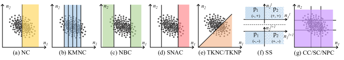
Figure 2: A schematic view of prior DNN coverage criteria. Aligned to Fig. 1, two axes denote two neurons in a layer.

NeuraL Coverage. Distributions formed by entangled neurons are important indicators of DNN behaviors. Given that “neural”, holistically, correlates to distributions of neuron outputs when understanding input features, this work proposes NeuraL Coverage, NLC, a new criterion that captures properties in distributions formed by neuron outputs. The term “neural,” as an adjective, better reflects that neuron outputs are processed in the continuous form and “L” also indicates each Layer is considered as the minimal computing unit.

III Motivation and Related Works

This section, by 1) comparing traditional software and DNN, 2) demonstrating limitations of prior criteria, and 3) incorporating practical considerations, proposes eight requirements for DNN coverage criteria that motivates NLC.

III-A DNN Testing and Software Testing

Discrete vs. Continuous States. Software coverage is often measured by counting #statements or #paths executed by an input. Software testing aims to maximize code coverage, as high coverage suggests comprehensive testing. Inspired by software testing, previous DNN testing often converts a neuron’s continuous outputs [33, 28], or distance between neuron output traces [22, 23], into discrete states. The coverage is denoted as the #activated states of a test input. As shown in Fig. 1, discrete states are unexpressive for describing neuron behavior. Instead, we advocate that a DNN coverage criterion should precisely describe the continuous output of a neuron.

Statement vs. Correlation. It is inaccurate to compare neurons to software statements, because each neuron is not an independent computing unit. In general, an “unactivated” neuron (defined by [33]) can still affect the DNN activities and final predictions. In contrast, software statements may not be covered by an input. Given that said, Fig. 1 shows that neuron outputs are often correlated (e.g., increasing simultaneously). Neuron correlation is, to some extent, analogous to program dependency, e.g., statements within an if block execute together. Rather than studying individual neurons, it is preferable (and more efficient) to measure DNN coverage by characterizing correlations of neurons.

Execution vs. Estimation. Software executes its input on an execution path. DNNs, as described in Sec. II, use a series of layers to approximate certain distributions for an input. Different DNN inputs produce different distributions, as seen in Fig. 1. Hence, we advocate to define the coverage criterion over approximated distributions. While it’s difficult to precisely describe the approximated distribution [34, 36, 48], certain informative properties of a distribution can be captured. Also, since coverage criteria are used to assess test suite quality and guide input mutations, knowing the exact distribution may not be required (see our empirical results in Sec. VI). In brief, we advocate that the DNN coverage criterion should analyze how outputs of neurons in a layer are distributed.

III-B Existing Neuron Coverage and Their Limitations

We illustrate existing DNN coverage criteria in Fig. 2 using two neurons to ease reading. In general, prior coverage criteria leverages discretization to decide if a state is “covered.”

Major Behavior of One Neuron. Neuron Coverage (NC) [33], as the first criterion, argues that the major behavior of a neuron is mostly reflected when its outputs are above zero. As in Fig. 2(a), NC deems a neuron as activated if its output is above threshold $T$ ($T$ is zero or a small value above). Following, three criteria were proposed [28], namely K-Multisection Neuron Coverage (KMNC), Neuron Boundary Coverage (NBC) and Strong Neuron Activation Coverage (SNAC). We display KMNC, NBC and SNAC in Fig. 2(b), Fig. 2(c) and Fig. 2(d). All three criteria first run training data to scope the output range of each neuron. Then, KMNC splits each range into $K$ segments and regards coverage as #segments covered by neuron outputs. NBC denotes coverage as #neuron outputs lying outside the range, while SNAC counts coverage as #neurons whose outputs are larger than the upper bound of its normal value range. Their intuition is that the major behaviors of neurons are denoted as outputs that lie in the range decided by training data.

Limitations: Considering the blue region in Fig. 1(c), it is easy to see that when feeding inputs of label “1”, NC over those two neurons will saturate. This indicates that criteria, which simply discretize neuron outputs, cannot properly describe the diversity of test suites (e.g., inputs of different labels). Moreover, since these criteria do not consider neuron entanglement, they should not change if the orange distribution of label “7” in Fig. 1(c) is rotated for 90 degrees. That is, these criteria might hardly reflect distinctly changed DNN behaviors.

Following , we argue that a neuron’s major behavior can hardly be defined using coarse-grained thresholds. Instead, given that the high-density regions formed by neuron outputs in a layer (e.g., the “dots” on Fig. 2’s background) are distinct on shapes, we deem the major behavior as the shapes which reflect the majority of neuron activates. Corner-case behaviors are therefore regarded as neuron outputs lying in low-density regions. In sum, we argue that DNN coverage should consider density of neuron output distributions. Measuring density considers both major and corner-case behaviors of DNNs, which is desirable in DNN testing.

Discretizing Outputs of Multiple Neurons. Two layer-wise criteria, Top-K Neuron Coverage (TKNC) and Top-K Neuron Patterns (TKNP), were also proposed in [28]. Both criteria denote a neuron as activated if its outputs are ranked at top-$K$ among neurons in a layer. TKNC counts #neurons once been activated, whereas TKNP records #patterns formed by activated neurons. As shown in Fig. 2(e) where there are two neurons, a neuron is activated if its output is greater than another one (i.e., $K=1$ and $n_{1}>n_{2}$). Sign-Sign coverage (SS) [43] captures the sign change of layer-wise adjacent neurons. A neuron is activated if 1) its outputs, and outputs from its adjacent neuron, have different signs for any pair of input $\langle p_{1},p_{2}\rangle$ (i.e., $n_{1}^{l}$ and $n_{1}^{l+1}$ in Fig. 2(f)) and simultaneously, 2) outputs from all other neurons in the same layer have an identical sign for $\langle p_{1},p_{2}\rangle$ (i.e., $n_{2}^{l}$ and $n_{2}^{l+1}$ in Fig. 2(f)).

Limitations: Despite considering all neurons in a layer, TKNC and TKNP still treat one neuron as a minimal computing unit and are incapable of analyzing the output distribution. They are easily saturated w.r.t. inputs of one or a few classes (see Fig. 1 and Fig. 2(e)), failing to assessing the diversity of a test suite. SS is specifically designed for ReLU-DNNs (i.e., DNNs with ReLU as the non-linear function). However, since most of the neuron outputs are nearly zero-centered due to input and layer normalization in modern DNNs [21, 42], SS can be less useful for many of them. Also, while SS considers the relation of adjacent layers, since each neuron is still a separate unit in SS, the relation of layers is modeled at the neuron-level.

As noted in Sec. II, the DNN hierarchy is formed by input feature re-use (e.g., processing shape at shallow layers and then texture at deep layers [14, 50]). The hierarchy is generally encoded into layer outputs. NLC, by capturing the distribution of layer outputs, is more desirable compared to SS.

Discretizing Distances over Traces of Neurons. Cluster-based Coverage (CC) assesses distances between traces of neuron outputs [32]. CC counts #clusters, where two clusters are formed if, the Euclidean distance of outputs from all neurons within a layer, is larger than a threshold. Given that more clusters are formed if neuron outputs get spread, CC can be regarded as counting #regions covered by several neuron outputs; as illustrated Fig. 2(g).

Surprise adequacy (SA) metrics, namely, Likelihood SA (LSA), Distance-ratio SA (DSA) and Mahalanobis Distance SA (MDSA), assess the distance between the neuron output trace of an input and neuron output traces of all training data to decide how “surprise” the new input is [22, 23]. LSA and DSA require iterating over all traces of neuron outputs collected from training data. MDSA reduces the computation cost by caching class-conditional mean and covariance matrices estimated on training data. Surprise Coverage (SC) derived via SAs discretizes the range of SA values into buckets, and coverage is denoted as the ratio of covered buckets.

Neuron Path Coverage (NPC) [46] is based on explainable AI techniques [2]: a path is constituted by critical neurons (identified via DNN gradients) from different layers. Similar to SCs, the coverage is calculated via discretized buckets of distance values over different paths. Holistically, since more spreading neuron outputs induce higher coverage values for SCs and NPC, they can also be expressed using Fig. 2(g).

Limitations: CC is more desirable than prior criteria given it is more comprehensive to overlay the output distribution. Nevertheless, CC could not capture correlations among neurons. SCs/NPC have similar limitations. In addition, unlike existing gray-box coverage criteria, NPC requires white-box access (e.g., DNN weights, back-propagation gradients) to the tested DNN, which limits its application scope.

III-C Practical Considerations

Incorporating Training Data. The training of a DNN involves a “test-and-fix” procedure: the DNN is tuned to reduce its errors and fit better on training data. This way, training data generally reflects how DNN works inside. We argue that DNN coverage should support incorporating prior-knowledge extracted from training data. Existing criteria use training data to scope neuron output ranges [28]. Nevertheless, for some criteria, e.g., TKNC/TKNP, their hyper-parameter $K$ depends on model structures instead of training data. NLC can use training data to estimate distributions of neuron outputs before being used in online testing, thereby satisfying .

Matrix-Form Computation. Coverage criteria are often used in costly DNN testing. According to the released code of existing criteria, we notice that they are mostly written in a loop-fashion which is slow. We find that testings guided by these criteria spend most time (over $80\%$) on coverage calculation. We re-implemented these criteria in a matrix-fashion, i.e., the calculation is performed as a sequence of matrix operations. Given that modern DL frameworks (e.g., PyTorch) can optimize matrix operations and also use hardware optimizations [10, 38, 29], the calculation is accelerated over $100$ times; see our codebase at [1]. Therefore, we advocate that a coverage criterion should support matrix-form computation to be optimizable by modern DL frameworks and hardware.

Incremental Update. DNN coverage is also typically used to guide test input mutations. Since inputs are gradually fed, we point out that a coverage should feature efficient incremental update. Ideally, when processing a new input, the cost for updating coverage should be a small constant. Since CC iterates over existing clusters and #clusters increases when more data are produced, it fails to fulfill . TKNP suffers from similar drawbacks. SS requires extensively comparing each neuron output with others and is thus inefficient for incremental update. Similarly, for each new input, LSC and DSC iterate over all neuron output traces of training data, resulting in a computing cost of the (#training data) $\times$ (#neurons) magnitude. Compared with other criteria (except for CC, TKNP, SS) which have a fixed small cost with a magnitude of (#neurons) for each incremental update, LSC and DSC fail to satisfy .

User-Friendliness. Most existing criteria rely on hyper-parameters. When using existing criteria, we find that coverage results are usually highly sensitive to hyper-parameters (see Sec. VI-A1), whereas existing works hardly provide guidance to decide hyper-parameters under different scenarios. Viewing that deciding hyper-parameters likely requires expertise (in both software testing and deep learning), we advocate that a DNN coverage is desirable to be hyper-parameter free.

TABLE I: Benchmarking coverage criteria for DNN testing. ✓, $\Diamond$, ✗ denote support, partially support, and not support. denotes gray-box (only needs neuron outputs) and denotes white-box that requires DNN weights and gradients.

NC [33]	✗	✗	✗	✗	✓	✓	✓	✗
KMNC [28]	✗	✗	✗	$\Diamond$	✓	✓	✓	✗
NBC [28]	✗	✗	✗	$\Diamond$	✓	✓	✓	✓
SNAC [28]	✗	✗	✗	$\Diamond$	✓	✓	✓	✓
TKNC [28]	✗	$\Diamond$	✗	✗	✗	✓	✓	✗
TKNP [28]	✗	$\Diamond$	✗	✗	✗	✓	✗	✗
SS [43]	✗	$\Diamond$	✗	✗	✗	✗	✗	✓
CC [32]	✗	✗	$\Diamond$	$\Diamond$	✓	✓	✗	✗
LSC [22]	✗	✗	$\Diamond$	$\Diamond$	✓	✓	✗	✗
DSC [22]	✗	✗	$\Diamond$	✗	✓	✓	✗	✗
MDSC [23]	✗	✗	$\Diamond$	✗	✓	✓	✓	✗
NPC [46]	✗	✗	$\Diamond$	$\Diamond$	✓	✓	✓	✗
NLC	✓	✓	✓	✓	✓	✓	✓	✓

III-D Comparison with Previous Criteria

Table I benchmarks existing DNN coverage criteria (and NLC) w.r.t. the eight requirements summarized in this section. Note that TKNC/TKNP consider the relative relation of neuron outputs and SS considers the sign relation between two neurons. They are deemed as partially satisfying . Though CC/SCs/NPC consider a trace of neurons, how one neuron responds to others can hardly be captured. They thus fail to satisfy . Given that the spreading of neuron outputs is captured, they partially fulfill . Also, since neuron outputs get concentrated, the neuron output range overlays the high-density regions. Similarly, the cluster/merged paths in CC/NPC and likelihood in LSC reflect high and low density regions respectively. We thus regard KMNC, NBC, SNAC, CC, and LSC as partially satisfying . In contrast, NLC satisfies all eight requirements, as explained in Sec. IV.

IV Design of NeuraL Coverage

As noted in Sec. III-A, it’s generally difficult to precisely and efficiently describe distributions approximated by DNNs [34, 36, 48]. Instead, as depicted in Fig. 3, NLC captures four key properties of distributions: divergence, correlation, shape, and density, which corresponds to the first four criteria in Table I. Sec. VI presents empirical results to show that these properties are sufficient to form a criterion that outperforms all existing works. We now elaborate on each property.

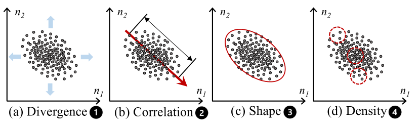
Figure 3: Four properties describing neuron output distributions. We take these properties into account to design NLC.

Measuring Activation in Continuous Space. Neuron outputs are continuous floating-point numbers. Instead of discretizing continuous neuron outputs, or distances between neuron output traces, NLC directly measures neuron outputs in the continuous space. We start with the case of one neuron.

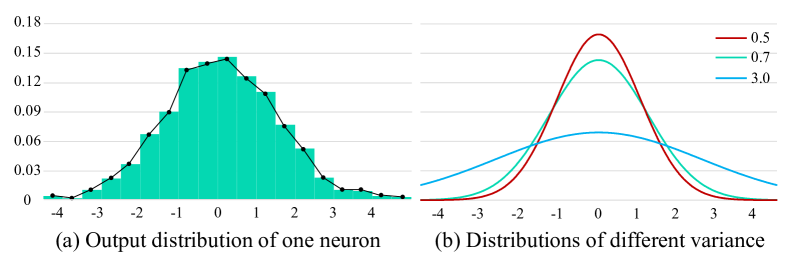
Figure 4: Output distribution of one neuron from ResNet50.

We randomly select one neuron from a pre-trained ResNet50 and plot its output distribution in Fig. 4(a) using all images in its training dataset. The x-axis denotes the output value and the y-axis denotes the ratio of involved inputs. Consistent with Fig. 1, output values converge to a certain point (zero in this case). NLC directly measures how divergent (i.e., how active) the neuron output is in its continuous form by calculating the following variance:

$$\sigma_{n}^{2}=\mathbb{E}[(o-\mathbb{E}[o])(o-\mathbb{E}[o])],$$ (1)

where $o$ is the output of a neuron $n$. Overall, variance is widely-adopted for characterizing the divergence of a collection of samples. Eq. 1 increases when output values spread along the x-axis. In contrast, if most outputs are zero, the variance will decrease, as in Fig. 4(b). Variance serves as an important descriptor of neuron output distributions. A test suite is regarded as comprehensive if it results in a high variance. Similarly, input mutations can be launched towards the direction that increases variance. Compared with previous criteria, we require no discretization, thus taking all distinct neuron outputs into account (in response to ). In addition, Eq. 1 does not ship with hyper-parameters (respond to ). It’s worth noting that variance is non-monotonic. That is, its value may decrease given new inputs. To alleviate this problem, we only update it when its value increases (i.e., $\Delta\sigma_{n}^{2}=\max(0,\Delta\sigma_{n}^{2})$). Generally, a stable variance, which stays constantly or tends to decrease, indicates that the behaviors are (nearly) fully explored.

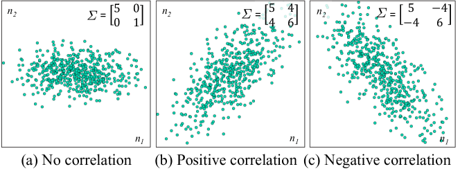
Figure 5: Neurons having various correlations.

Characterizing Neuron Correlation. As noted in Sec. II, neurons in a layer are entangled and jointly process input features. As empirically assessed in Fig. 1, neurons manifest distinct correlations under different tasks and for inputs of different classes. For example, in Fig. 1(c), neuron $n_{1}$ is positively (e.g., class “1”) or negatively (e.g., class “9”) correlated with neuron $n_{2}$.

Fig. 5 presents three different correlations of two neurons. Given that there are more than one neuron, the DNN coverage should simultaneously consider the divergence of each neuron and correlations among neurons. Eq. 1 uses variance to describe divergence of a neuron’s output, i.e., $\sigma^{2}_{n_{1}}$ and $\sigma^{2}_{n_{2}}$. Similarly, we use the covariance, a common metric for joint variability of two variables, to characterize the correlation between two neurons. Thus, the correlation between the two neurons is formulated as

$$\varsigma_{n_{1},n_{2}}=\mathbb{E}[(n_{1}-\mathbb{E}[n_{1}])(n_{2}-\mathbb{E}[n_{2}])]=\varsigma_{n_{2},n_{1}}.$$ (2)

$\varsigma_{n_{1},n_{2}}=0$ implies that $n_{1}$ and $n_{2}$ are not correlated, whereas $\varsigma_{n_{1},n_{2}}>0$ denotes a positive correlation between $n_{1}$ and $n_{2}$, i.e., $n_{1}$ will increase with $n_{2}$, and vice verse. A higher $\varsigma_{n_{1},n_{2}}$ denotes a stronger correlation. The same holds when $\varsigma_{n_{1},n_{2}}<0$. Taking Eq. 1 and Eq. 2 into account, we simultaneously represent the divergence of each neuron and correlations of neurons in a unified form as

$$\varSigma=\begin{bmatrix}\sigma^{2}_{n_{1}}&\varsigma_{n_{1},n_{2}}\\ \varsigma_{n_{2},n_{1}}&\sigma^{2}_{n_{2}}\end{bmatrix},$$ (3)

where $\varSigma$ is the covariance matrix of $n_{1}$ and $n_{2}$. As we show in Fig. 5, the value of $\varsigma_{n_{1},n_{2}}$ also represents the divergence along the “correlation direction” of two neurons. Thus, we use

$$\frac{1}{m\times m}\|\varSigma\|_{1}=\frac{1}{m\times m}\sum\nolimits_{j=1}^{m}\left(\sum\nolimits_{i=1}^{m}|\varsigma_{n_{i},n_{j}}|\right),$$ (4)

where $m$ is #neurons and $\varsigma_{n_{i},n_{i}}=\sigma^{2}_{n_{i}}$, to represent the DNN coverage. The size of $\varSigma$ is $m\times m$ and $\frac{1}{m\times m}$ works as the normalization term to eliminate the effect of #neurons to the coverage values. In the case where more than two neurons are correlated, e.g., $n_{i}$, $n_{j}$ and $n_{k}$, $\varSigma$ will characterize the correlation via $\varsigma_{n_{i},n_{j}}$, $\varsigma_{n_{i},n_{k}}$ and $\varsigma_{n_{j},n_{k}}$. Hence, Eq. 4 facilitates addressing requirements  and . Note that $\varSigma$ can be initialized using the correlation term $\varsigma_{n_{i},n_{i}}$ decided by training data. Also, $\varSigma$ can be further refined in a class conditional manner by extending the size to $c\times m\times m$ where $c$ is #classes. It thus will be calculated by first being indexed using the class labels. In both two cases, NLC fulfills the requirement of . Further, given a DNN contains multiple layers, the coverage of DNN is computed as

$$\textsc{NLC}\ =\sum_{l}\frac{1}{m^{l}\times m^{l}}\|{\varSigma}^{l}\|_{1},$$ (5)

where $l$ is the layer index. A higher NLC indicates a more diverse test suite. Test input mutations, accordingly, are expected to accumulate towards directions that maximize NLC.

Capturing Distribution Shape. Unlike previous works where each neuron is considered separately, we take neurons from the same layer as a group. As in Fig. 1, the output distribution of neurons in the same layer is mostly distinct under different tasks. Moreover, for the separated regions (in different colors) under certain tasks (e.g., classification), they may also have different shapes characterizing various DNN behaviors. Hence, we capture a major behavior by describing the shape of a distribution. We now explain why $\varSigma$ in Eq. 3 captures a distribution’s shape.

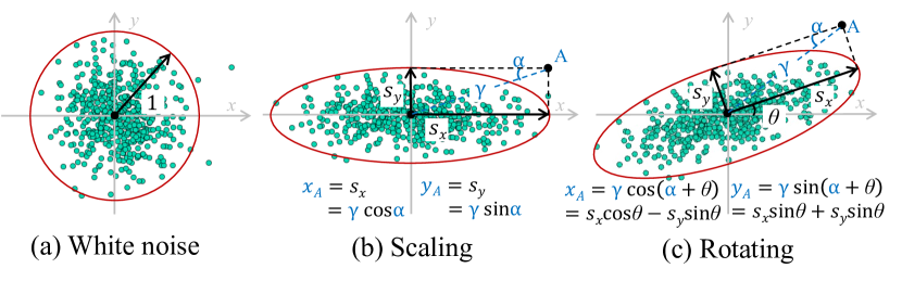
Figure 6: Transforming white noise to a desired distribution.

To ease understanding, we first show how to transform a white noise (whose covariance matrix is degenerated into an identity matrix $I$) to the distribution formed by outputs from a group of neurons. Fig. 6(a) shows a white noise $\mathcal{N}$ and Fig. 6(c) presents the output distribution of two neurons $x$ and $y$. The transformation is thus decomposed into two elementary operators — scaling and rotating. The scaling operator spreads two neuron outputs and rotating introduces correlations between $x$ and $y$. Rotating and scaling are defined by rotation matrix and scaling matrix as

$$\mathcal{R}_{2\times 2}=\begin{bmatrix}\cos\theta&-\sin\theta\\ \sin\theta&\cos\theta\\ \end{bmatrix},\mathcal{S}_{2\times 2}=\begin{bmatrix}s_{x}&0\\ 0&s_{y}\\ \end{bmatrix},$$ (6)

respectively. Thus, the output distribution can be represented as $(\mathcal{R}\mathcal{S})\mathcal{N}$. Following Eq. 1 and Eq. 2, we have

$$\varSigma =\mathbb{E}[(\mathcal{R}\mathcal{S}\mathcal{N}-\mathbb{E}[\mathcal{R}\mathcal{S}\mathcal{N}])(\mathcal{R}\mathcal{S}\mathcal{N}-\mathbb{E}[\mathcal{R}\mathcal{S}\mathcal{N}])^{\top}]$$ (7)

$$=(\mathcal{R}\mathcal{S})\mathbb{E}[(\mathcal{N}-\mathbb{E}[\mathcal{N}])(\mathcal{N}-\mathbb{E}[\mathcal{N}])^{\top}](\mathcal{R}\mathcal{S})^{\top}$$

$$=(\mathcal{R}\mathcal{S})I(\mathcal{R}\mathcal{S})^{\top}=(\mathcal{R}\mathcal{S})(\mathcal{R}\mathcal{S})^{\top},$$

which indicates that covariance matrix $\varSigma$ in Eq. 3 encodes transformations from a white noise to a desired distribution. Therefore, we demonstrate that $\varSigma$ captures the shape (i.e., how it is distributed) of the output distribution formed by outputs of neurons in a layer, satisfying .

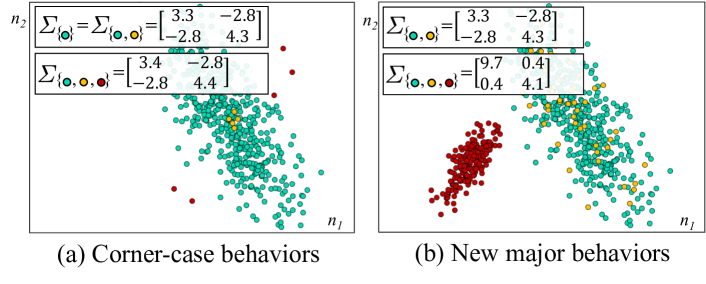
Figure 7: Responses to density changes.

Responding to Density Change. Neuron outputs generally concentrate to certain points to form clusters, and the density varies in the output space. We first elaborate on what may introduce a local density change. Recall that we deem corner-case behaviors as neuron outputs lying at the low-density regions (e.g., boundary of one cluster), which are likely to trigger DNN defects. Given that these outliers typically have much lower local-density, their existence will lead to density change. Consider Fig. 7(a) where the DNN outputs in red are deemed as outliers. Nevertheless, since they are still in the output ranges formed by all green dots, SNAC and NBC will not treat them as corner case behaviors. In fact, the new red outputs will not induce coverage increase for all previous criteria except CC and SCs, because CC and SCs capture how neuron outputs spread in the whole space. However, they require properly selected distance thresholds, which are hyper-parameters configured by users.

Also, for certain cases where neuron outputs are separated (e.g., the classifier in Fig. 1(c)), the appearance of a new major behavior (e.g., images get classified as a new class) also leads to density change. As in Fig. 7(b), the new cluster of red dots introduces a new major behavior, whereas NC possibly has no response since their values are lower than the threshold.

We show that NLC responds to density change. For Fig. 7(a), the $||\varSigma||_{1}$ of existing green dots is $13.2$. It will be updated as $13.4$ given the new red dots, which indicates that NLC responds. In contrast, since the new yellow dots stay close to the majority of existing outputs, NLC has no response. It’s worth mentioning that, despite the density changes only slightly, NLC has no resolution loss given its continuous form. Meanwhile, for Fig. 7(b), the $||\varSigma||_{1}$ will change from $13.2$ to $14.6$ when the cluster formed by red dots appears. We thus state that our criterion can respond to density change which is possibly introduced by corner-case behaviors and new major behaviors. This way, NLC satisfies .

Clarification on Covariance. Both MDSC and NLC rely on covariance. We, however, clarify that the two “covariances” imply distinct concepts. NLC characterizes how fresh inputs change the neuron correlation or introduce new distributions, using an actively-updated covariance. NLC incrementally updates covariance given new inputs and rollbacks the value if the new input is not desired. In contrast, the covariance in MDSC is a pre-computed constant that represents the distribution of historical neuron outputs, based on which the Mahalanobis distance can be computed from.

Implementation Considerations. As discussed above, it is easy to see that NLC supports matrix-form computing and has no hyper-parameter. Thus, NLC satisfies  and . We now clarify that NLC supports incremental computing (requirement of ). We also show that NLC supports batch computation, which is also vital as DNNs generally take a batch of inputs and the batch size varies from $1$ to hundreds. Let existing data be $\mathbb{B}$, given a batch of new data $B$, the covariance matrix $\varSigma$ (Eq. 4) of each layer can be calculated as

$$\varSigma =\frac{|\mathbb{B}|\times|B|\times(\mu_{\mathbb{B}}-\mu_{B})(\mu_{\mathbb{B}}-\mu_{B})^{\top}}{(|\mathbb{B}|+|B|)^{2}}$$ (8)

$$+\frac{|\mathbb{B}|\times\varSigma_{\mathbb{B}}+|B|\times\varSigma_{B}}{|\mathbb{B}|+|B|},$$

where $\mu$ is the mean of a collection of data. Clearly, Eq. 8 does not iterate over existing data and the computing cost is in a magnitude of (#neurons); NLC thus satisfies .

V Implementation and Configurations

NLC is implemented using PyTorch (ver. 1.9.0) with roughly 2,300 LOC. All experiments are launched on one Intel Xeon CPU E5-2683 with 256GB RAM and one Nvidia GeForce RTX 2080 GPU. Below we briefly introduce settings of prior criteria compared with NLC. Their implementations are released in [1].

Optimization and Hyper-parameters. We perform optimizations on our end for all prior criteria examined in Sec. VI in order to report their best results. In original SCs, coverage is calculated as the ratio of covered buckets. More specifically, given the maximal SA value $U$ and maximal bucket count $m$, SCs first discretize $U$ as $m$ buckets of size $\frac{U}{m}$, then, they calculate coverage as the ratio of covered bucket (by test suites) over the total $m$ buckets. Nevertheless, our preliminary study shows that it is uneasy to tune these two parameters, $U$ and $m$, separately. Thus, we use the bucket size $T=\frac{U}{m}$, which represents $U$ and $m$ with only one variable $T$, as the hyper-parameter for tuning. Accordingly, we report the number of covered buckets in Sec. VI, which is equivalent to the original ratio of covered buckets. Suppose our reported coverage value is $|S|$, which denotes the number of elements in $S$ and $S$ is the set of indexes of covered buckets. To convert it into the ratio used in original SCs, users need to first choose a maximal SA value $U$, and obtain $S^{\prime}=\{s|Ts\leq U,s\in S\}$. The ratio of covered buckets can be computed as $\frac{T|S^{\prime}|}{U}\%$.

Additionally, as described in Sec. III-B, we re-implement the prior criteria’s calculation in a matrix form to boost their computation efficiency. We denote the hyper-parameters of KMNC, TKNC, and TKNP as $K$ in Sec. VI. In other criteria, thresholds are denoted as $T$.

SS and NPC. SS is specifically designed for ReLU-DNN, whereas modern DNNs have various non-linear functions which are not supported by SS. Also, SS does not support matrix-form and incremental computing. Our preliminary study shows that it is computational infeasible due to the large number of neurons in modern DNN. NPC requires white-box DNN, which is not always practical in testing scenarios. In addition, its building block, the layer-wise propagation [2], is only applicable to discriminative models. We thus omit to compare with them.

VI Evaluation

VI-A Assessing Test Suite Quality

We first compare NLC with existing criteria on its effectiveness to assess the 1) diversity and 2) fault-revealing capability of test suites.

Settings & DNNs & Datasets. We evaluate NLC on both discriminative and generative models. The involved models and datasets are listed in Table II and Table III. For discriminative models, we choose VGG16, ResNet50, and MobileNetV2, which represent standard large-scale DNNs with sequential and non-sequential topological structures and popular models on mobile platforms. The three models are trained on two datasets of different scales, namely, CIFAR10 [25] and ImageNet [11]. Models trained on CIFAR10 have over $92\%$ test accuracy and those trained on ImageNet are provided by PyTorch. CIFAR10 is composed of $32\times 32$ images labeled as ten classes. ImageNet contains images of $1,000$ classes and the average image size is $469\times 387$. We also evaluate NLC on the text model, i.e., a LSTM [19] trained on the IMDB dataset [30] for sentiment analysis [13]. Given that each layer in the LSTM is unrolled to process sequential inputs, the unrolled layers are considered separately for computing coverage [44]. For generative models, we choose the SOTA model BigGAN. The BigGAN is also trained on CIFAR10 and ImageNet.

Forming Ground Truth. In practice, it is infeasible to compare coverage values to the ground truth (e.g., a test suite covers 70% of all “diversity” which is inaccessible due to the infinite number of possible inputs in the wild). Besides, the coverage value is hardly interpretable (see discussion in Sec. VII). Consequently, the expected magnitude of the coverage induced by a test suite is unknown. To overcome these hurdles, we construct cases where the relative order of coverage values induced by different test suites is quantifiable (e.g., which test suite results in relatively larger coverage). The relative order forms a reasonable and measurable ground truth against which coverage values can be compared to determine their accuracy.

VI-A1 Diversity of Test Suites

Discriminative Models. To assess the diversity of test suites for discriminative models, we construct two datasets of different diversity using schemes denoted as $\times 1$ and $\times 10$. For the $\times 1$ scheme, we randomly choose $100$ images from the test data and add white noise to produce dummy images (the total number of dummy images in $\texttt{test}_{\times 1}$ equals to the size of all test data). The white noise is truncated within $[-0.1,0.1]$ to preserve the appearance of images. Given that text is discrete, it is infeasible to add white noise. We thus randomly shuffle words in the $100$ selected sentences to produce dummy sentences. The $\times 10$ scheme follows the same procedure, but the number of the dummy data is $10$ times of the test data.

Ground Truth (Table IV and Table V): The diversity of these datasets are ranked as $\texttt{test}>\texttt{test}_{\times 10}>\texttt{test}_{\times 1}$, because test contains over 10K diverse and meaningful samples in real-world datasets, whereas $\texttt{test}_{\times 10}$ and $\texttt{test}_{\times 1}$ are generated by (slightly) mutating 100 data samples.

TABLE II: DNN Models used in Sec. VI-A. All image models are trained on CIFAR10 and ImageNet.

Model	#Neuron	#Layer	Remark
ResNet50 [17]	26,570/27,560	54	Non-sequential topology
VGG16_BN* [41]	12,426/13,416	16	Sequential topology
MobileNet-V2 [20]	17,066/18,056	53	Mobile devices
BigGAN [8]	6,403/48,627	11/41	Generative model
LSTM [19]	32,769	129	Text model

• *All image models have batch normalization (BN) layers.

TABLE III: Datasets (train/test) used in Sec. VI-A. Each class has the same number of images.

Dataset	CIFAR10	ImageNet	IMDB
#Classes	10	1,000	2
#Data	50,000/10,000	1,000,000/50,000	17,500/17,500

TABLE IV: Coverage achieved by different (text) test suites on LSTM. Assessments matching ground truth are marked.

Criteria	Config.	IMDB	$\text{IMDB}_{\times 10}$	$\text{IMDB}_{\times 1}$
NC ($\%$)	$T$=$0.25$	0.012	0.034	0.018
	$T$=$0.50$	0.015	0.027	0.018
	$T$=$0.75$	2.191	2.554	1.001
KMNC ($\%$)	$K$=$10$	7.68	12.11	3.69
	$K$=$100$	1.92	5.31	2.99
	$K$=$1,000$	0.05	0.15	0.08
NBC ($\%$)	N/A	0.12	0.13	0.04
SNAC ($\%$)	N/A	0.11	0.03	0.03
TKNC ($\%$)	$K$=$1$	0.28	0.67	0.19
	$K$=$10$	0.50	0.96	0.39
	$K$=$50$	1.34	2.86	1.20
TKNP ($\#$)	$K$=$1$	20,252	101,789	12,118
	$K$=$10$	6,515	8,602	2,224
	$K$=$50$	11,830	20,479	4,633
CC ($\#$)	$T$=$10$	266	283	265
	$T$=$20$	134	146	137
	$T$=$50$	57	65	1
LSC ($\#$)	$T$=$1$	306	314	214
	$T$=$10$	40	60	27
	$T$=$100$	5	7	7
DSC ($\#$)	$T$=$0.01$	176	185	153
	$T$=$0.1$	25	24	18
	$T$=$1$	4	4	4
MDSC ($\#$)	$T$=$1$	101	229	97
	$T$=$10$	18	43	22
	$T$=$100$	4	5	5
NLC	N/A	1279.81	132.99	11.01

TABLE V: Coverage achieved by different (image) test suites on discriminative models. CR and IN denote CIFAR10 and ImageNet dataset, respectively. Assessments matching ground truth are marked.

Criteria	Config.	ResNet						VGG						MobileNet
		CR	$\texttt{CR}_{\times 10}$	$\texttt{CR}_{\times 1}$	IN	$\texttt{IN}_{\times 10}$	$\texttt{IN}_{\times 1}$	CR	$\texttt{CR}_{\times 10}$	$\texttt{CR}_{\times 1}$	IN	$\texttt{IN}_{\times 10}$	$\texttt{IN}_{\times 1}$	CR	$\texttt{CR}_{\times 10}$	$\texttt{CR}_{\times 1}$	IN	$\texttt{IN}_{\times 10}$	$\texttt{IN}_{\times 1}$
NC ($\%$)	$T$=$0.25$	0.026	0.031	0.031	0	0	0	0.113	0.225	0.177	0	0	0	0	0	0	0	0	0
	$T$=$0.5$	0.75	2.10	1.14	0	0.01	0	0.56	1.09	0.77	0	0.01	0	0.02	0.05	0.01	0	0	0
	$T$=$0.75$	2.15	4.54	2.52	0.13	0.38	0.21	2.49	4.27	3.25	0.02	0.02	0	1.57	2.17	1.69	0.02	0.03	0.02
KMNC ($\%$)	$K$=$10$	8.89	40.50	40.01	4.10	5.59	4.25	7.33	55.50	55.25	4.19	9.17	8.34	8.53	10.43	8.97	4.67	6.82	4.52
	$K$=$100$	8.52	28.37	26.96	2.17	5.14	5.08	7.54	45.60	45.25	1.36	5.26	5.22	4.81	10.19	10.02	1.43	3.01	2.15
	$K$=$1,000$	3.99	10.78	10.64	1.87	4.31	4.29	2.84	12.50	12.36	0.91	2.68	2.61	4.61	8.69	8.38	2.01	3.92	3.44
NBC ($\%$)	N/A	0	4.85	1.75	0.13	1.20	0.48	0.27	2.12	2.04	0.08	0.23	0.13	0.003	2.51	2.46	0.15	0.32	0.20
SNAC ($\%$)	N/A	0	2.62	0.97	0.14	0.73	0.57	0.53	1.64	1.52	0.13	0.23	0.01	0	2.37	1.41	0.15	0.38	0.27
TKNC ($\%$)	$K$=$1$	0.20	0.41	0.23	0.06	0.10	0.03	0.81	1.97	1.20	0.29	0.44	0.13	0.24	0.28	0.13	0.10	0.20	0.06
	$K$=$10$	0.38	0.68	0.36	0.11	0.14	0.02	2.29	3.83	2.66	0.01	0.01	0.01	0.21	0.31	0.12	0.03	0.03	0.03
	$K$=$50$	0.24	0.45	0.23	0.03	0.06	0.01	3.07	4.57	3.35	0.01	0.02	0.02	0.17	0.38	0.22	0.02	0.05	0
TKNP ($\#$)	$K$=$1$	9,995	80,561	9,586	4,900	23,384	3,954	6,060	36,887	6,809	4,882	17,187	3,386	9,998	90,537	9,924	4,900	48,083	5,000
	$K$=$10$	10,000	100,000	10,000	4,901	50,000	5,000	10,000	100,000	10,000	4,901	50,000	5,000	10,000	100,000	10,000	4,901	50,000	5,000
	$K$=$50$	1,034	1,823	434	4,901	50,000	5,000	10,000	100,000	10,000	4,901	50,000	5,000	694	1,665	650	4,901	50,000	5,000
CC* ($\#$)	$T$=$10$ / $T$=$1,000$	55	60	44	4,945	9,787	1,333	147	168	137	14,532	7,681	2,148	37	38	29	4,947	43,613	4,614
	$T$=$20$ / $T$=$2,000$	19	23	19	4,918	9,771	397	51	63	48	11,914	1,606	954	9	11	10	4,946	12,466	2,618
	$T$=$50$ / $T$=$5,000$	9	9	7	4,130	8,263	256	22	22	21	4,526	571	426	7	7	4	4,943	531	346
LSC** ($\#$)	$T$=$1$ / $T$=$100$	196	628	423	1,475	2095	1,373	400	1,153	671	1,243	2,070	1,028	164	553	574	2,028	3,118	1,858
	$T$=$10$ / $T$=$500$	44	69	83	414	502	420	79	117	98	357	447	275	36	51	48	610	755	545
	$T$=$100$ / $T$=$1,000$	7	7	8	227	214	228	10	13	12	199	223	201	5	7	6	256	359	335
DSC ($\#$)	$T$=$0.01$	489	3,478	831	Failed			566	6,431	1,120	Failed			471	4,491	1,742	Failed
	$T$=$0.1$	146	426	307	Failed			253	4,983	565	Failed			148	1,276	460	Failed
	$T$=$1$	34	39	54	Failed			107	1,195	110	Failed			42	161	75	Failed
MDSC ($\#$)	$T$=$1$	422	987	675	Failed			639	4,065	1,538	Failed			651	1,023	733	Failed
	$T$=$10$	73	93	100	Failed			208	780	365	Failed			176	400	279	Failed
	$T$=$100$	7	10	9	Failed			50	110	87	Failed			38	31	42	Failed
NLC	N/A	1.03	0.47	0.05	6006.38	113.37	11.00	403.95	0.004	0	20327.50	413.50	49.50	0.61	0.23	0.12	10693.50	757.25	86.25

• *$T\in\{10,20,50\}$ for CIFAR10 (CR) and $T\in\{1000,2000,5000\}$ for ImageNet (IN).

• **$T\in\{1,10,100\}$ for CIFAR10 (CR) and $T\in\{100,500,1000\}$ for ImageNet (IN).

TABLE VI: Coverage achieved by different datasets on generative models. CR and IN refer to BigGAN trained on CIFAR10 and ImageNet. Assessments matching ground truth are marked.

Criteria	Config.	DNN	Normal	${N/2}$	${N/10}$	${C/2}$	${C/10}$
NC ($\%$)	$T$=$0.25$	CR	99.97	99.97	99.95	99.97	99.95
		IN	99.43	99.42	99.40	99.42	99.39
	$T$=$0.5$	CR	99.34	99.30	99.02	99.25	98.73
		IN	94.18	93.96	93.44	93.87	93.44
	$T$=$0.75$	CR	86.66	84.88	79.70	82.85	76.90
		IN	81.64	81.30	80.17	80.98	77.61
KMNC ($\%$)	$K$=$10$	CR	54.72	56.00	54.71	54.24	52.44
		IN	58.15	57.06	58.14	56.20	56.82
	$K$=$100$	CR	21.54	21.45	21.84	21.83	21.48
		IN	22.66	22.33	22.59	22.20	22.32
	$K$=$1000$	CR	3.04	3.04	3.04	3.04	3.03
		IN	3.07	3.08	3.07	3.07	3.06
NBC ($\%$)	N/A	CR	0.22	0.09	0.04	0.09	0.10
		IN	0.54	0.21	0.21	0.03	0.06
SNAC ($\%$)	N/A	CR	0.02	0.03	0.03	0.03	0.03
		IN	0.03	0.07	0.04	0.64	0.14
TKNC ($\%$)	$K$=$1$	CR	31.69	27.75	16.95	27.16	15.56
		IN	16.79	14.56	9.62	13.11	5.91
	$K$=$10$	CR	62.64	58.89	48.34	58.46	45.14
		IN	34.92	33.77	29.90	32.44	22.62
	$K$=$50$	CR	83.96	81.45	75.03	81.23	73.54
		IN	42.02	41.68	40.58	41.27	38.08
TKNP ($\#$)	$K$=$1$	CR	31,415	15,843	3,193	15,779	3,134
		IN	32,000	16,000	3,200	16,000	3,200
	$K$=$10$	CR	32,000	16,000	3,200	16,000	3,200
		IN	32,000	16,000	3,200	16,000	3,200
	$K$=$50$	CR	32,000	16,000	3,200	16,000	3,200
		IN	10,894	6,898	2,088	6,997	2,178
CC ($\#$)	$T$=$50$	CR	347	302	175	232	89
		IN	1,204	921	485	780	324
	$T$=$100$	CR	90	70	40	50	18
		IN	323	266	147	239	108
	$T$=$200$	CR	27	25	13	23	7
		IN	105	99	77	95	64
LSC ($\#$)	$T$=$1$ $T$=$100$	CR	1,286	1,047	627	1,011	607
		IN	197	154	63	153	48
	$T$=$10$ $T$=$500$	CR	216	188	136	181	122
		IN	92	68	27	61	27
	$T$=$100$ $T$=$1,000$	CR	40	32	20	37	21
		IN	66	42	14	43	17
DSC ($\#$)	$T$=$0.01$	CR	123	111	90	90	74
		IN	412	325	184	317	167
	$T$=$0.1$	CR	13	13	12	12	10
		IN	76	56	39	67	31
	$T$=$1$	CR	2	2	2	2	2
		IN	10	9	7	10	7
MDSC ($\#$)	$T$=$1$	CR	249	232	97	260	89
		IN	943	673	418	640	401
	$T$=$10$	CR	24	19	18	17	24
		IN	224	188	119	222	122
	$T$=$100$	CR	3	4	3	2	2
		IN	119	47	15	45	32
NLC	N/A	CR	1051.63	776.29	653.62	280.67	178.92
		IN	3596.89	3306.88	3141.02	2636.64	1462.11

Generative Models. Generative models generate images by sampling from a fixed distribution (i.e., the normal distribution). Since this procedure is conditioned on a given class label, we construct datasets of different diversity by following the $Normal$, $N/x$ and $C/x$ schemes (see Table VI). For the $Normal$ scheme, we sample total $m$ inputs from the normal distribution and each class has the same number of inputs. For the $N/x$ scheme, we only keep $1/x$ of inputs from each class, whereas for the $C/x$ scheme, we only keep $1/x$ of classes. We set $m$ to $32,000$ and choose $x\in\{2,10\}$.

Ground Truth (Table VI): Since inputs conditioned on different classes are all sampled from normal distribution, behaviors of generative models are primarily decided by the class labels. Thus, the diversity of these datasets are ranked as: $Normal>N/2>N/10>C/2>C/10$.

Result Overview. We show the increased coverage of different test suites compared with training data (since the DNN is already “tested” using its training data) in Table IV, Table V and Table VI for text (discriminative) models, image (discriminative) models, and generative models, respectively. All experiments are launched for five times to reduce randomness. The maximum deviations are around $0.01\%$ and $1$ for criteria in $\%$ and $\#$ units, respectively.

Scalability Issues of MDSC/DSC. In Table V, we only evaluate MDSC/DSC using CIFAR10. MDSC requires storing class-conditional covariance matrices, whose space cost is $O(\text{\#class}\times{\text{\#neuron}}^{2})$. Note that ImageNet has 1K classes and 1M training data (Table III). DSC takes over 12 hours to assess one scheme of ImageNet (criteria satisfying  only take several minutes) since it iterates over 1M neuron output traces for each test input. It’s thus infeasible to apply MDSC/DSC on models trained on ImageNet that is much larger than CIFAR10.

Impacts of Hyper-parameters. Previous criteria (except for NBC and SNAC) require extra hyper-parameters, which largely affect the results. For instance, in Table V, all variants of CIFAR10 test data have nearly zero coverage when $T$ of NC is $0.25$, whereas they reach a saturation coverage when $K$ of TKNP is $10$ (i.e., #patterns equals to #inputs) despite they are still evaluated on same models. Moreover, the hyper-parameter $T$ of CC is model specific, for instance, $T=10$ is suitable for ResNet trained on CIFAR10, but is too small if the ResNet is trained on ImageNet — any input will form a new cluster. We thus increase $T$ 100 times for models trained on ImageNet. SCs suffer from the similar issue (e.g., LSC in Table V) even though we have optimized the hyper-parameter configurations. Before applying these criteria, users need to scope the distance range for each model. Again, without prior knowledge on setting hyper-parameters, it is obscure to adopt these criteria in real-life usage. In contrast, NLC is hyper-parameter free, enabling an “out-of-the-box” usage.

Discriminative Model: Quantity, not Diversity. For most cases in Table IV and Table V, the $\times 1$ scheme and the test dataset have comparable results, and the $\times 10$ scheme has the highest coverage. Given datasets created by $\times 1$ have an identical size with the test dataset, we interpret that previous neuron coverage criteria are more sensitive to the number of data samples rather than the diversity. Nevertheless, the coverage assessed by NLC is consistent with the diversity of these datasets (i.e., the ground truth). Moreover, despite the number of $\times 10$ variant is 10 times of test data, its reflected coverage on NLC is smaller, indicating that NLC successfully reflects input diversity.

Discriminative Model: Dissimilarity, not Diversity. We note that in most cases, SCs have $\text{test}_{\times 1}>\text{test}$. Recall that SCs primarily describe how distinct a test input is towards training data. This implies that SCs are more sensitive to the dissimilarity rather than the diversity of test suites. Also, though CC and SCs are conceptually similar to some extent, we find that CC has relatively better performance. CC represents coverage as #clusters based on Euclidean distance, in contrast, SCs focus on designing new distance metrics. To compute coverage, SCs simply discretize the distance values as buckets. From this comparison, it might not be inaccurate to interpret that how to represent coverage based on the distance may be more essential than the distance metric itself.

Generative Models: the Incapability. To train generative models like BigGAN, inputs for both training and test phases are random variables sampled from the normal distribution (here, training images act as “labels”). Infinite “training inputs” exist, and therefore, KMNC, NBC, SNAC and SCs are infeasible to use, as they require to first obtain neuron outputs using all training inputs. Practically, we use all samples from $Normal$ schemes to simulate the training inputs. Nevertheless, we find that coverage values measured by them are random (e.g., the “CR” row of SNAC in Table VI). In contrast, NLC, by default, can be used with no training data, and it can be adopted in both discriminative and generative models.

Generative Models: Quantity, not Diversity. For the remaining coverage criteria, most of their results are ranked as $Normal>N/2>C/2>N/10>C/10$, which further reflects that prior criteria are more sensitive to the number of inputs instead of their diversity. Since previous criteria consider neurons separately, feeding more inputs might increase the chance of activating more neurons or producing a distinct trace of neuron outputs. In contrast, NLC analyzes the entanglements among neurons, where most “trivial” inputs will not influence the correlations or distributions. Since a diverse test suite possibly uncovers different neuron correlations, NLC becomes more responsible for a diverse test suite.

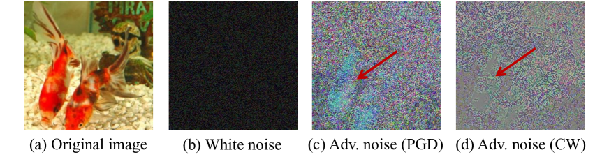
Figure 8: Adversarial perturbations.

TABLE VII: Coverage achieved by test data and AEs of CIFAR10$\dagger$. Assessments matching ground truth are marked.

	Data	NC	KMNC	NBC	SNAC	TKNC	TKNP	CC	LSC	DSC	MDSC	NLC
		$0.75$	$100$			$10$	$50$	$10$	$10$	$0.1$	$10$
		($\%$)	($\%$)	($\%$)	($\%$)	($\%$)	($\#$)	($\#$)	($\#$)	($\#$)	($\#$)
R	Test	2.15	8.52	0	0	0.38	1,034	55	44	146	73	1.0
	CW	0.90	0	3.94	2.73	0.18	31	5	0	336	0	2.4
	PGD	1.43	0	13.83	23.22	0.35	680	29	115	785	372	22.9
V	Test	2.49	7.54	0.27	0.53	2.29	10,000	147	79	253	208	403.9
	CW	0.20	0	5.03	7.08	0.20	9,542	125	0	949	0	931.0
	PGD	1.69	0.74	12.64	15.23	1.32	4,997	142	222	5,901	1,461	4749.1
M	Test	1.57	4.81	0	0	0.21	694	37	36	148	176	0.6
	CW	0.02	0	1.77	1.62	0.14	172	13	0	452	0	0.9
	PGD	0.36	0	9.71	10.39	0.16	299	16	65	3,648	97	13.6

• $\dagger$ R, V, M denote ResNet, VGG, MobileNet, respectively.

TABLE VIII: Coverage achieved by AEs generated (via PGD) using test data of CIFAR10$\dagger$. Assessments matching ground truth are marked.

Model	NC	KMNC	NBC	SNAC	TKNC	TKNP	CC	LSC	DSC	MDSC	NLC
	$0.75$	$100$			$10$	$50$	$10$	$10$	$0.1$	$10$
	($\%$)	($\%$)	($\%$)	($\%$)	($\%$)	($\#$)	($\#$)	($\#$)	($\#$)	($\#$)
ResNet	0.41	0	9.17	13.04	0.16	980	20	0	590	323	8.60
VGG	0.58	0	12.40	14.90	0.44	4,999	94	0	3,044	917	1584.4
MobileNet	0.20	0	2.30	3.10	0.17	639	12	0	2,808	86	10.43

VI-A2 Fault-Revealing Capability of Test Suites

Setup. To evaluate the fault-revealing capabilities of test suites, we construct adversarial examples (AE) using two adversarial attack algorithms, Carlini/Wagner (CW) [9] and Project Gradient Descent (PGD) [31]. CW and PGD are two representative types of algorithms for AE generation, namely, optimization-based and loss function-based. Perturbations added on AEs are different from white noise, as shown in Fig. 8, which generally highlight objects in images. AEs are generated using the training data (see “Clarification” below for results of AEs generated using test data), and all algorithms attacking the three models reach over $98\%$ success rates. That is, more than $0.98\times\text{(\#training data)}$ AEs can trigger erroneous behaviors. The incorrect predictions uniformly distribute across all classes.

Ground Truth (Table VII): Since the AE set manifests a higher fault-revealing capability (also discloses more untested cases), it should have a higher coverage value. Thus, the ground in this evaluation is PGD $>$ Test, or CW $>$ Test.

Result Overview. As with the previous settings, we record and present the increased coverage of test data and AEs in Table VII. NC, TKNC, TKNP and CC have higher coverage for the test data than AEs, indicating that they are unable to assess the fault-revealing capability of a test suite. Harel-Canada et al. [16] also find that NC is not strongly correlated with defect detection, which is aligned with our results. Nevertheless, Table VII shows that NLC is strongly and positively correlated to the fault-revealing capability of a test suite.

Implementation Issues of LSC. MDSC has zero coverage on AEs generated using CW. Generally, perturbations added by CW are harder to identify [9]. This statement can also be illustrated by Table VII (nearly all coverage values of PGD are much higher than CW) and Fig. 8. Though LSC also gives zero coverage for CW AEs, it is seemingly due to some numerical issues. In particular, we observed some inf (infinite numbers) when LSC was computing the Gaussian kernel to measure the “surprise” of a test input. AE may induce a large neuron output, which consequently result in inf since exponential functions ($f(x)=e^{x}$) are used by the Gaussian kernel. DSC shows generally promising results for this evaluation, giving higher coverage values for AEs than normal test inputs.

Correlation to “Out-of-Bound” Neuron Outputs. KMNC has no response to AEs, but NBC and SNAC respond notably, because AEs primarily lead to out-of-range neuron outputs. NLC measures how divergent a layer output is and responds to the density change of layer outputs. Therefore, the out-of-range neuron outputs, which either induce a higher variance or introduce a low-density layer output, can be captured.

Clarification. Using training data to generate AEs helps alleviate side effects caused by the diversity of test data. To clarify, AEs generated using training data should not introduce new semantical content, because AEs retain patterns in the training data except several stealthily mutated pixels (e.g., a cat in a seed image still appears in the resulting AE). Therefore, if the coverage increases, it shows the fault-revealing capability. Nevertheless, if we use AEs generated by the test dataset, it is hard to determine if the increase is due to unseen semantical content on AEs (because test inputs are unseen by DNNs), or due to the fault-revealing capability. We also report results on AEs generated using test data in Table VIII, whose findings are generally consistent with Table VII.

TABLE IX: Coverage achieved by adversarial-perturbed inputs (AP; not AE) generated using test data of CIFAR10$\dagger$. Assessments matching ground truth are marked.

	PGD				CW
	NBC	SNAC	DSC	NLC	NBC	SNAC	DSC	NLC
			$0.1$				$0.1$
	($\%$)	($\%$)	($\#$)		($\%$)	($\%$)	($\#$)
ResNet	0	0	463 $>$ Test	0.20	3.33 $>$ Test	2.30 $>$ Test	0	0.13
VGG	0	0	1,295 $>$ Test	48.35	2.06 $>$ Test	4.30 $>$ Test	52	36.21
MobileNet	0	0	427 $>$ Test	0.06	1.12 $>$ Test	1.70 $>$ Test	0	0.02

Adversarial Perturbations. While NBC/SNAC/DSC appear to match all ground truth in Table VII, we suspect that they respond to the adversarial perturbations instead of the fault-revealing capability of AEs. This is derived from the following controlled experiments. We first randomly pick 1,000 inputs from the test set (which has 10,000 inputs). Then, we add adversarial-perturbations (CW/PGD) on these inputs but do not change their predictions (they are thus not AE). Let these adversarial-perturbed inputs be AP. We compare the increased coverage of AP vs. test dataset (Test).

The ground truth (Table IX) should be: $0<\text{AP}<\text{Test}$. AP $<$ Test because AP do not lead to mispredictions, but Test is ten times larger than AP. 0 $<$ AP because AP has 1,000 inputs of diverse semantical contents. Results are in Table IX. NLC has correct results for all settings, and DSC only matches ground truth for $\langle\text{VGG}\&\text{CW}\rangle$. NBC/SANC fail in all settings.

This is an important observation, indicating that NBC/SNAC/DSC do not accurately reflect the fault-revealing capability. Instead, they are sensitive to the “dissimilarity” induced by adversarial perturbations (even if Test is 10$\times$ larger than AP). As introduced in Sec. III-B, NBC/SNAC increase if an input triggers neuron output lying outside the output range decided by the training data. That is, if an input is more dissimilar to training data, it is more likely to increase NBC/SNAC. Also, DSC increases the coverage if an input has a large distance (measured using DSA) to neuron outputs of training data.

VI-B Guiding Input Mutation in DNN Testing

This section uses existing criteria and NLC as the objective to guide input mutation. This denotes a typical feedback-driven (fuzz) testing setting, where inputs are mutated to maximize the feedback yielded by the criteria. We evaluate the mutated inputs on 1) #triggered faults, 2) naturalness, and 3) diversity of the erroneous behaviors.

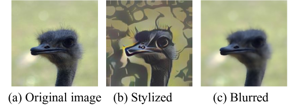
Figure 9: Stylizing and blurring.

Setup. We use the same image classification models and datasets as in Sec. VI-A. Table XI and Table XI list mutation methods and configurations of coverage criteria. In sum, mutations in Table XI are representative, for example, blurring and stylizing (see Fig. 9) reveal the texture-bias (i.e., rely on texture to make decisions) of DNNs [14, 7].

We launch fuzzing using either prior coverage criteria or NLC as in Alg. 1. $terminate()$ returns True when reaching 10K iterations or exceeding $6$ hours. $is\_valid()$ is adopted from [47], which deems a mutation as valid if 1) the #changed-pixels is less than $\alpha\times$ #pixels or 2) the maximum of changed pixel value is less than $\beta\times 255$. We set $\alpha$ to $0.2$ and $\beta$ to $0.4$. As a baseline, we do not check validity and coverage (line 7 in Alg. 1) for random mutation. That is, line 7 in Alg. 1 always yields true for random mutation. We randomly select 1K inputs from the test dataset as the fuzzing seeds.

TABLE X: Transformations.

Type	Operator	Remark
Pixel-Level	contrast, brightness	Robustness
Affine	translation, scaling, rotation	Shape bias
Texture-Level	blurring, stylizing	Texture bias

TABLE XI: Config.

DSC: $0.1$	NC: $0$
MDSC: $10$	LSC: $10$
TKNC: $10$	KMNC: $100$
TKNP: $50$	CC: $10/1000$

1 Transformation Set: $\mathcal{T}$; Fuzzing Seed: $S$;

2 Tested DNN: $D$; Criterion: $C$; $num\leftarrow 50$;

3 while not terminate() do

4       $s=sample(\mathcal{S})$;

5       for $i\leftarrow 0$ to $num$ by $1$ do

6             $t=sample(\mathcal{T})$; $\hat{s}\leftarrow t(s)$;

7             if $is\_valid(\hat{s},s)$ and $coverage\_inc(C,D)$ then

8                   $S.add(\hat{s})$; $update\_coverage(C)$;

9                   break;

10                  

Algorithm 1 Fuzzing algorithm.

TABLE XII: Fuzzing results. Faults, Outputs, Entropy denote triggered faults, fuzzing outputs, scaled entropy, respectively.

		#Faults/#Outputs	IS	FID	#Classes	Entropy
CIFAR10	Rand	4,730/10,000	5.08	185.59	10	0.75
	NC	1,063/1,817	4.65	176.57	10	0.94
	KMNC	0/0	N/A	N/A	0	0
	NBC	8/10	1.99	415.01	4	0.91
	SNAC	5/8	2.70	469.29	1	0
	TKNC	844/1,458	5.36	183.73	10	0.93
	TKNP	5,983/9,380	5.30	170.19	10	0.85
	CC	37/52	2.55	358.93	10	0.92
	LSC	73/93	2.64	350.67	9	0.84
	DSC	743/889	4.45	234.68	10	0.85
	MDSC	210/284	2.96	279.24	9	0.58
	NLC	8,716/10,000	5.61	167.87	10	0.97
ImageNet	Rand	6,448/10,000	8.05	131.85	595	0.82
	NC	3,309/4,157	8.05	99.35	672	0.91
	KMNC	0/0	N/A	N/A	0	0
	NBC	5/6	1.85	367.84	4	0.96
	SNAC	8/10	2.62	372.49	7	0.97
	TKNC	3,127/3,967	7.82	99.87	668	0.90
	TKNP	7,190/10,000	7.77	101.08	711	0.87
	CC	7,902/10,000	7.13	102.84	708	0.86
	LSC	7,246/10,000	7.74	100.38	700	0.79
	DSC	24/31	2.54	278.55	17	0.93
	MDSC	N/A	N/A	N/A	N/A	N/A
	NLC	9,975/10,000	8.14	98.87	732	0.88*

• *Higher Entropy is better if two #Classes are equal, otherwise, higher #Classes is better.

Triggered Faults. The #triggered faults of ResNet trained on CIFAR10 and ImageNet are presented in Table XII. DSC is unsuitable to be an objective, because its computing cost impedes fuzzing throughput (the fuzzer mutates images for only a few times within 6 hours). Images mutated under the guidance of NLC (last row) have the highest error triggering rates compared with random mutation (3rd row) and other criteria, especially NBC, SNAC, KMNC. Recall that these criteria denote a neuron as activated if its output is higher than a threshold or is out-of-range. Since modern DNNs frequently perform normalization, neuron outputs tend to concentrate to certain regions (as reflected in Fig. 1). Without fine-grained feedbacks such as gradients, mutated images can hardly flip an unactivated neuron into activated. Nevertheless, we find that the degree of entanglement among neurons can vary w.r.t. mutated inputs. Thus, NLC is very effective to serve the fuzzing guidance, achieving the highest #faults and fault-triggering rates. TKNP and CC have decent performance, since the patterns and clusters in TKNP and CC, to some extent, can reflect the neuron entanglement.

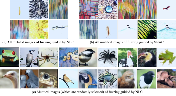
Figure 10: Mutated images of fuzzing guided by different criteria.

Naturalness of Mutations. Contemporary testing works have pointed out the importance of preserving naturalness of mutated images [16]. We measure the naturalness of mutated inputs under each criterion; a good criterion should lead to mutations that mostly preserve the naturalness. We use Inception Score (IS) [39] and Fr$\grave{e}$chet Inception Distance (FID) [18], which are widely used in the AI and SE community to assess the naturalness of images, as the metrics. A higher IS score is better, whereas a lower FID score indicates better naturalness. The evaluation results are also listed in Table XII.

Random mutation’s IS and FID scores are the baselines. Overall, mutated images guided by NLC have the best scores for both IS and FID. Mutated images guided by SCs, NBC, SNAC have relatively low naturalness. SCs prefer inputs that are distinct to training data (also pointed out in Sec. VI-A1). Given the high comprehensiveness of real-world datasets, SCs may likely push to produce unrecognizable images. NBC and SNAC denote a neuron as activated if it has out-of-range outputs. Thus, its guided mutations tend to largely modify pixel values. We find that the mutated images become less recognizable; Fig. 10 shows their mutated outputs on ImageNet. Overall, since neurons jointly process features in an image, mutations guided by NLC, which aims to cover different neuron entanglements, are holistically “bounded” by features — the mutated images (see Fig. 10) thus have better visual quality.

Diversity of Erroneous Behaviors. A higher diversity of erroneous behaviors indicates uncovering a practically larger vulnerability surface of DNN models. Overall, a collection of fault-triggering images are regarded as more diverse if they cover more classes. In case that #covered classes is equal, we further use the scaled entropy, $-\frac{1}{|C|}\sum p_{c}\log p_{c}$ where $p_{c}$ is the ratio of incorrect outputs predicted as class $c$ and $|C|$ is the #classes, to assess the diversity: a higher entropy is better. The results are also presented in Table XII. It is seen that fault-triggering images generated by using NLC as the guidance cover the most classes. We thus envision equipping fuzz testing frameworks with NLC to likely identify more and diverse defects from real-world critical DNN systems.

VII Discussion

TABLE XIII: Time cost for 10K CIFAR10 inputs on ResNet.

NC	KMNC	NBC	SNAC	TKNC	TKNP	CC	LSC	DSC	MDSC	NLC
2.3s	8.3s	2.4s	2.3s	3.6s	431.5s	75.9s	37.3s	432.5s	14.3s	4.4s

Time/Space Cost of NLC. Table XIII compares the time cost of NLC with previous criteria. NLC is slower than NC/NBC/SNAC/TKNC due to covariance computation. It is slightly faster than KMNC/MDSC and much faster than TKNP/CC/LSC/DSC.

Despite both MDSC [23] and NLC use covariance matrix, NLC requires less memory space. Let $m_{i}$ be #neurons in the $i$-th DNN layer and $K$ be #classes in training data, NLC takes $\sum_{i}m^{2}_{i}$ space, while MDSC takes $K\times(\sum_{i}m_{i})^{2}$. To interpret the comparison: first, $K$ is large in real-world datasets ($K=1000$ in ImageNet), hence MDSC may be hardly used on ImageNet-trained DNNs but NLC can. Second, when $K$ is $1$, NLC still takes less space and saves more space for deeper DNNs.

Interpretability and Usage. We view that DNN coverage criteria (including NLC and prior works) may share common limitation of shallow interpretability on their outcomes; For instance, as noted in Sec. III-B, NC simplifies the neuron output (a continuous value) to a binary state (activated vs. unactivated). Hence, given a case of 100% NC coverage, we are concerned that different neuron output values and the combination states of neurons/layers are far from fully examined. Worse yet, once it hits 100% (merely CIFAR10 training data can have 100% coverage on ResNet using $\langle\text{NC},T=0.2\rangle$), further tests cannot be guided by NC. That is, “saturating” state of DNN criteria should not be interpreted as revealing all DNN behaviors. Similarly, zero coverage reported by some criteria does not imply that DNN behaviors are never explored. In Table V, when using the same inputs (CIFAR10), NBC has zero coverage, whereas $\langle\text{TKNP},K=10\rangle$ is saturated (increases 10,000 with 10,000 inputs).

High-level speaking, DNN coverage is not simply analogous to software coverage, where each statement is either “covered” or not. Outputs of DNN coverage criteria depend on how those criteria, not merely the DNNs, are designed/implemented. Fundamentally, neuron outputs are continuous, and neurons in DNN layers collaborate to comprehend the semantics of high-dimensional inputs (e.g., images). Explaining DNN decisions is still an open problem. Thus, DNN coverage is not as clear as traditional software coverage, where we simply “count” if a statement/path/basic block is covered or not.

In sum, aligned with recent criteria like CC [32], we do not strive to establish a “maximal value” for NLC (since misprediction cannot be eliminated currently). To use NLC, developers should try their best to maximize NLC values with test inputs. Also, it is infeasible to universally decide the number of inputs required to maximize NLC, as this number depends on the DNN structures, weights, and training data.

VIII Conclusion

Given observations that DNNs approximate distributions, we propose eight design requirements for DNN testing criteria. We design NLC, a criterion that fulfills all requirements. NLC considers the continuity, correlation, distribution, and density of layer outputs in a DNN. It also enables various optimizations. We show that NLC can facilitate test input assessment and serve as guidance of fuzz testing with better performance.

References

- [1] Research artifact. https://github.com/Yuanyuan-Yuan/NeuraL-Coverage.
- [2] Sebastian Bach, Alexander Binder, Grégoire Montavon, Frederick Klauschen, Klaus-Robert Müller, and Wojciech Samek. On pixel-wise explanations for non-linear classifier decisions by layer-wise relevance propagation. PloS one, 10(7):e0130140, 2015.
- [3] Richard Bellman. Dynamic programming. Science, 153(3731):34–37, 1966.
- [4] Yoshua Bengio, Aaron Courville, and Pascal Vincent. Representation learning: A review and new perspectives. IEEE transactions on pattern analysis and machine intelligence, 35(8):1798–1828, 2013.
- [5] Christopher M Bishop et al. Neural networks for pattern recognition. Oxford university press, 1995.
- [6] Hans-Dieter Block. The perceptron: A model for brain functioning. Reviews of Modern Physics, 34(1):123, 1962.
- [7] Wieland Brendel and Matthias Bethge. Approximating cnns with bag-of-local-features models works surprisingly well on imagenet. arXiv preprint arXiv:1904.00760, 2019.
- [8] Andrew Brock, Jeff Donahue, and Karen Simonyan. Large scale gan training for high fidelity natural image synthesis. In International Conference on Learning Representations, 2018.
- [9] Nicholas Carlini and David Wagner. Towards evaluating the robustness of neural networks. In 2017 ieee symposium on security and privacy (sp), pages 39–57. IEEE, 2017.
- [10] Tianqi Chen, Thierry Moreau, Ziheng Jiang, Lianmin Zheng, Eddie Yan, Haichen Shen, Meghan Cowan, Leyuan Wang, Yuwei Hu, Luis Ceze, et al. TVM: An automated end-to-end optimizing compiler for deep learning. In 13th USENIX Symposium on Operating Systems Design and Implementation (OSDI 18), pages 578–594, 2018.
- [11] Jia Deng, Wei Dong, Richard Socher, Li-Jia Li, Kai Li, and Li Fei-Fei. Imagenet: A large-scale hierarchical image database. In 2009 IEEE conference on computer vision and pattern recognition, pages 248–255. Ieee, 2009.
- [12] Li Deng. The mnist database of handwritten digit images for machine learning research [best of the web]. IEEE Signal Processing Magazine, 29(6):141–142, 2012.
- [13] Ronen Feldman. Techniques and applications for sentiment analysis. Communications of the ACM, 56(4):82–89, 2013.
- [14] Robert Geirhos, Patricia Rubisch, Claudio Michaelis, Matthias Bethge, Felix A. Wichmann, and Wieland Brendel. Imagenet-trained CNNs are biased towards texture; increasing shape bias improves accuracy and robustness. In International Conference on Learning Representations, 2019.
- [15] Ian Goodfellow, Jean Pouget-Abadie, Mehdi Mirza, Bing Xu, David Warde-Farley, Sherjil Ozair, Aaron Courville, and Yoshua Bengio. Generative adversarial nets. In Advances in neural information processing systems, pages 2672–2680, 2014.
- [16] Fabrice Harel-Canada, Lingxiao Wang, Muhammad Ali Gulzar, Quanquan Gu, and Miryung Kim. Is neuron coverage a meaningful measure for testing deep neural networks? In Proceedings of the 28th ACM Joint Meeting on European Software Engineering Conference and Symposium on the Foundations of Software Engineering, pages 851–862, 2020.
- [17] Kaiming He, Xiangyu Zhang, Shaoqing Ren, and Jian Sun. Deep residual learning for image recognition. In Proceedings of the IEEE conference on computer vision and pattern recognition, pages 770–778, 2016.
- [18] Martin Heusel, Hubert Ramsauer, Thomas Unterthiner, Bernhard Nessler, and Sepp Hochreiter. Gans trained by a two time-scale update rule converge to a local nash equilibrium. In Advances in neural information processing systems, pages 6626–6637, 2017.
- [19] Sepp Hochreiter and Jürgen Schmidhuber. Long short-term memory. Neural computation, 9(8):1735–1780, 1997.
- [20] Andrew G Howard, Menglong Zhu, Bo Chen, Dmitry Kalenichenko, Weijun Wang, Tobias Weyand, Marco Andreetto, and Hartwig Adam. Mobilenets: Efficient convolutional neural networks for mobile vision applications. arXiv preprint arXiv:1704.04861, 2017.
- [21] Sergey Ioffe and Christian Szegedy. Batch normalization: Accelerating deep network training by reducing internal covariate shift. In International conference on machine learning, pages 448–456. PMLR, 2015.
- [22] Jinhan Kim, Robert Feldt, and Shin Yoo. Guiding deep learning system testing using surprise adequacy. In ICSE, 2019.
- [23] Jinhan Kim, Jeongil Ju, Robert Feldt, and Shin Yoo. Reducing dnn labelling cost using surprise adequacy: An industrial case study for autonomous driving. In Proceedings of the 28th ACM Joint Meeting on European Software Engineering Conference and Symposium on the Foundations of Software Engineering, pages 1466–1476, 2020.
- [24] Diederik P Kingma and Max Welling. Auto-encoding variational bayes. arXiv preprint arXiv:1312.6114, 2013.
- [25] Alex Krizhevsky, Geoffrey Hinton, et al. Learning multiple layers of features from tiny images. 2009.
- [26] Hsin-Ying Lee, Hung-Yu Tseng, Jia-Bin Huang, Maneesh Singh, and Ming-Hsuan Yang. Diverse image-to-image translation via disentangled representations. In Proceedings of the European conference on computer vision (ECCV), pages 35–51, 2018.
- [27] Yu Liu, Fangyin Wei, Jing Shao, Lu Sheng, Junjie Yan, and Xiaogang Wang. Exploring disentangled feature representation beyond face identification. In Proceedings of the IEEE Conference on Computer Vision and Pattern Recognition, pages 2080–2089, 2018.
- [28] Lei Ma, Felix Juefei-Xu, Jiyuan Sun, Chunyang Chen, Ting Su, Fuyuan Zhang, Minhui Xue, Bo Li, Li Li, Yang Liu, et al. DeepGauge: Comprehensive and multi-granularity testing criteria for gauging the robustness of deep learning systems. In Proceedings of the 33rd ACM/IEEE International Conference on Automated Software Engineering, ASE 2018.
- [29] Lingxiao Ma, Zhiqiang Xie, Zhi Yang, Jilong Xue, Youshan Miao, Wei Cui, Wenxiang Hu, Fan Yang, Lintao Zhang, and Lidong Zhou. Rammer: Enabling holistic deep learning compiler optimizations with rtasks. In 14th USENIX Symposium on Operating Systems Design and Implementation (OSDI 20), pages 881–897, 2020.
- [30] Andrew Maas, Raymond E Daly, Peter T Pham, Dan Huang, Andrew Y Ng, and Christopher Potts. Learning word vectors for sentiment analysis. In Proceedings of the 49th annual meeting of the association for computational linguistics: Human language technologies, pages 142–150, 2011.
- [31] Aleksander Madry, Aleksandar Makelov, Ludwig Schmidt, Dimitris Tsipras, and Adrian Vladu. Towards deep learning models resistant to adversarial attacks. arXiv preprint arXiv:1706.06083, 2017.
- [32] Augustus Odena and Ian Goodfellow. Tensorfuzz: Debugging neural networks with coverage-guided fuzzing. arXiv preprint arXiv:1807.10875, 2018.
- [33] Kexin Pei, Yinzhi Cao, Junfeng Yang, and Suman Jana. DeepXplore: Automated whitebox testing of deep learning systems. In Proceedings of the 26th Symposium on Operating Systems Principles, SOSP ’17, pages 1–18, New York, NY, USA, 2017. ACM.
- [34] Carl Edward Rasmussen et al. The infinite gaussian mixture model. In NIPS, volume 12, pages 554–560. Citeseer, 1999.
- [35] Jie Ren, Mingjie Li, Zexu Liu, and Quanshi Zhang. Interpreting and disentangling feature components of various complexity from dnns. In International Conference on Machine Learning, pages 8971–8981. PMLR, 2021.
- [36] Douglas A Reynolds. Gaussian mixture models. Encyclopedia of biometrics, 741:659–663, 2009.
- [37] Frank Rosenblatt. The perceptron: a probabilistic model for information storage and organization in the brain. Psychological review, 65(6):386, 1958.
- [38] Nadav Rotem, Jordan Fix, Saleem Abdulrasool, Garret Catron, Summer Deng, Roman Dzhabarov, Nick Gibson, James Hegeman, Meghan Lele, Roman Levenstein, et al. Glow: Graph lowering compiler techniques for neural networks. arXiv preprint arXiv:1805.00907, 2018.
- [39] Tim Salimans, Ian Goodfellow, Wojciech Zaremba, Vicki Cheung, Alec Radford, and Xi Chen. Improved techniques for training gans. Advances in neural information processing systems, 29:2234–2242, 2016.
- [40] Jürgen Schmidhuber. Deep learning in neural networks: An overview. Neural networks, 61:85–117, 2015.
- [41] Karen Simonyan and Andrew Zisserman. Very deep convolutional networks for large-scale image recognition. arXiv preprint arXiv:1409.1556, 2014.
- [42] Jorge Sola and Joaquin Sevilla. Importance of input data normalization for the application of neural networks to complex industrial problems. IEEE Transactions on nuclear science, 44(3):1464–1468, 1997.
- [43] Youcheng Sun, Xiaowei Huang, Daniel Kroening, James Sharp, Matthew Hill, and Rob Ashmore. Testing deep neural networks. arXiv preprint arXiv:1803.04792, 2018.
- [44] Yuchi Tian, Kexin Pei, Suman Jana, and Baishakhi Ray. DeepTest: Automated testing of deep-neural-network-driven autonomous cars. ICSE ’18, 2018.
- [45] Shuai Wang and Zhendong Su. Metamorphic object insertion for testing object detection systems. In ASE, 2020.
- [46] Xiaofei Xie, Tianlin Li, Jian Wang, Lei Ma, Qing Guo, Felix Juefei-Xu, and Yang Liu. Npc: N euron p ath c overage via characterizing decision logic of deep neural networks. ACM Transactions on Software Engineering and Methodology, 2022.
- [47] Xiaofei Xie, Lei Ma, Felix Juefei-Xu, Hongxu Chen, Minhui Xue, Bo Li, Yang Liu, Jianjun Zhao, Jianxiong Yin, and Simon See. Coverage-guided fuzzing for deep neural networks. arXiv preprint arXiv:1809.01266, 2018.
- [48] Guorong Xuan, Wei Zhang, and Peiqi Chai. Em algorithms of gaussian mixture model and hidden markov model. In Proceedings 2001 International Conference on Image Processing (Cat. No. 01CH37205), volume 1, pages 145–148. IEEE, 2001.
- [49] Yuanyuan Yuan, Qi Pang, and Shuai Wang. Revisiting neuron coverage for dnn testing: A layer-wise and distribution-aware criterion. ICSE, 2023.
- [50] Matthew D Zeiler and Rob Fergus. Visualizing and understanding convolutional networks. In European conference on computer vision, pages 818–833. Springer, 2014.
- [51] Mengshi Zhang, Yuqun Zhang, Lingming Zhang, Cong Liu, and Sarfraz Khurshid. DeepRoad: GAN-based Metamorphic Testing and Input Validation Framework for Autonomous Driving Systems. In ASE, 2018.