Towards Low-loss 1-bit Quantization of User-item Representations for Top-K Recommendation

Abstract.

Due to the promising advantages in space compression and inference acceleration, quantized representation learning for recommender systems has become an emerging research direction recently. As the target is to embed latent features in the discrete embedding space, developing quantization for user-item representations with a few low-precision integers confronts the challenge of high information loss, thus leading to unsatisfactory performance in Top-K recommendation. In this work, we study the problem of representation learning for recommendation with 1-bit quantization. We propose a model named Low-loss Quantized Graph Convolutional Network (L²Q-GCN). Different from previous work that plugs quantization as the final encoder of user-item embeddings, L²Q-GCN learns the quantized representations whilst capturing the structural information of user-item interaction graphs at different semantic levels. This achieves the substantial retention of intermediate interactive information, alleviating the feature smoothing issue for ranking caused by numerical quantization. To further improve the model performance, we also present an advanced solution named L²Q-GCN_anl with quantization approximation and annealing training strategy. We conduct extensive experiments on four benchmarks over Top-K recommendation task. The experimental results show that, with nearly 9$\times$ representation storage compression, L²Q-GCN_anl attains about $90$$\sim$$99\%$ performance recovery compared to the state-of-the-art model.

1. Introduction

Recommender systems (RSs), as a useful tool to perform personalized information filtering (Covington et al., 2016; Hamilton et al., 2017), nowadays play a critical role throughout various Web applications, e.g., social networks, E-commerce platforms, and streaming media websites. Learning vectorized user-item representations (a.k.a. embeddings) for prediction has become the core of modern recommender systems (He et al., 2020; Cheng et al., 2018; He et al., 2017). Among existing techniques, graph-based methods, i.e., Graph Convolutional Networks (GCNs), due to the ability of capturing high-order relations in user-item interaction topology, well simulate the collaborative filtering process and thus produce a remarkable semantic enrichment to the user-item representations (Wang et al., 2019; Sun et al., 2019; Hamilton et al., 2017; He et al., 2020).

Apart from the representation informativeness, space overhead is another important criterion for realistic recommender systems. With the explosive growth of interactive data encoded in the graph form, quantized representation learning recently provides an alternative option to GCN-based recommender methods for optimizing the model scalability. Generally, quantization is the process of converting a continuous range of vectorized values into a finite discrete set, e.g., integers. Instead of using continuous embeddings, e.g., 32-bit floating points, 1-bit quantization however embeds user-item latent features into the binary embedding space, e.g., $\{-1,1\}^{d}$. By enabling the usage of low-precision integer arithmetics, 1-bit quantized representations have the promising potential in space compression and inference acceleration for recommendation (Tailor et al., 2021).

Figure 1. Illustration of conventional quantized CNN and semantic propagation within the user-item interaction graph.

Despite the previous attempts to quantize traditional model-based RS methods (Zhang et al., 2016, 2017; Kang et al., 2021), quantizing graph-based RS models (Tan et al., 2020) however receive less attention so far. Due to their unique message passing mechanism (Hamilton et al., 2017; Kipf and Welling, 2017) in encoding high-order interactive information, it is emerging as a good research topic to study representation quantization for GCN-based recommender models. Currently, it is still challenging to approach this target as previous work falls short of satisfaction in terms of recommendation accuracy. The crux of this phenomenon is mainly twofold:

• Intuitively, the performance degradation for quantizing representations is mainly caused by the limited expressivity of discrete embeddings. Different from applications in other domains, e.g., Natural Language Processing, Computer Vision (Bennett, 1948; Gersho and Gray, 2012; Bai et al., 2021), the top principle of quantization for recommendation is ranking preserving. However, compared to full-precision embeddings, the vectorized latent features of both users and items tend to be smoothed by the discreteness of quantization naturally. For instance, after the quantization into binary embedding space $\{-1,1\}^{d}$, only the digit signs are kept, no matter what specific values of continuous embeddings originally are. Consequently, this leads to the information loss when estimating users’ preferences towards different items, thus drawing a conspicuous performance decay in ranking tasks, e.g., Top-K recommendation.

• Technically, previous work mainly takes inspiration from the methodology of Quantized Convolutional Neural Networks (Qin et al., 2020; Rastegari et al., 2016; Lin et al., 2017) (illustrated in Figure 1(a)) to plug quantization as a separate encoder that is posterior to the GCN architecture. Being the final encoder for object embeddings (i.e., users and items), this however ignores the intermediate representations when graph convolution performs on the sub-structures of interaction graphs. As pointed out by (Wang et al., 2019), the intermediate information at different layers of graph convolution is important to reveal different semantics of user-item interactions. For example, as shown in Figure 1(b), when lower-layers propagate information between users and items that have historical interactions, higher-layers capture higher-order proximity of users (or items). Hence, ignoring intermediate semantics fails to the feature enrichment for embedding quantization. Furthermore, due to the “double-edged” effect of GCN, final embeddings at the last graph convolution layer may be over-smoothed (Li et al., 2018; Li et al., 2019) to become uninformative accordingly. This implies that simply using the output embeddings may be risky and problematic (He et al., 2020), which leads to the suboptimal quantized representations for recommendation.

In this paper, we investigate the problem of 1-bit quantized representation learning for recommendation with the GCN framework. We propose a model named Low-loss 1-bit Quantized Graph Convolutional Network (L²Q-GCN). L²Q-GCN interprets the user-item representations in the discrete space $\{-1,1\}^{d}$. We design the quantization-based graph convolution such that L²Q-GCN achieves the embedding quantization whilst capturing different levels of interactive semantics in exploring the user-item interaction graphs. Intuitively, such topology-aware quantization makes the user-item representations more comprehensive, and thus significantly alleviates the information loss of numerical quantization that causes the performance decay. Specifically, we propose two solutions, namely L²Q-GCN_end and L²Q-GCN_anl, to provide flexibility towards different deployment scenarios. We conduct extensive experiments on four benchmarks over Top-K recommendation task. To summarize, our main contributions are as follows:

1. We implement our proposed network design in L²Q-GCN_end that is trained in an end-to-end manner. Our experimental results demonstrate that, L²Q-GCN_end achieves nearly 11$\times$ representation compression and about 40% inference acceleration, while retaining over $80$% recommendation capacity, compared to the state-of-the-art full-precision model.

2. To further improve the recommendation performance, we propose an advanced solution L²Q-GCN_anl with approximation that is trained by a two-step annealing training strategy. With slightly additional space cost, L²Q-GCN_anl can attain $90$$\sim$$99\%$ performance recovery.

3. We release codes and datasets to researchers via the link (our, [n.d.]) for reproducing and validating.

Organization. We first review the related work in Section 2 and present L²Q-GCN_end and L²Q-GCN_anl in Sections 3 and 4. We report the experimental results on four benchmarks in Section 5 and conclude the paper in Section 6.

2. Related Work

2.1. Full-precision GCN-based RS Models

Recently, GCN-based recommender systems have become new state-of-the-art methods for Top-K recommendation (He et al., 2020; Wang et al., 2019), thanks to their capability of capturing semantic relations and topological structures for user-item interactions (Kipf and Welling, 2017; Hamilton et al., 2017; Zhang et al., 2019). Motivated by the advantage of graph convolution, prior work such as GC-MC (Berg et al., 2017), PinSage (Ying et al., 2018) and recent state-of-the-art models NGCF (Wang et al., 2019) and LightGCN (He et al., 2020) are proposed. Generally, they adapt the GCN framework to simulate the collaborative filtering process in high-order graph neighbors for recommendation. For example, NGCF (Wang et al., 2019) follows the GCN-based information propagation rule to learn embeddings: feature transformation, neighborhood aggregation, and nonlinear activation. LightGCN (He et al., 2020) further simplifies the graph convolution by retaining the most essential GCN components to achieve further improved recommendation performance. In our experiments, we settle these two state-of-the-art full-precision methods as the benchmarking reference for L²Q-GCN in Top-K recommendation.

2.2. General Binarized GCN Frameworks

Network binarization (Hubara et al., 2016) aims to binarize all parameters and activations in neural networks so that they can even be trained by logical units of CPUs. Binarized models will dramatically reduce the memory usage. Despite the progress of binarization CNNs (Rastegari et al., 2016; Qin et al., 2020) for multimedia retrieval, this technique is not adequately studied in geometric deep learning (Wang et al., 2021; Bahri et al., 2021; Wu et al., 2021). Bi-GCN (Wang et al., 2021) and BGCN (Bahri et al., 2021) are two recent trials. However, they are mainly designed for geometric classification tasks, but their capability of link prediction (a geometric form of recommendation) is unclear. Furthermore, compared to focusing on the quantization for user-item representations only, a complete network binarization will further abate the numerical expressivity of modeling ranking information for recommendation. This implies that a direct adaptation of binary GCN models may draw large performance decay in Top-K recommendation.

2.3. Quantization-based RS Models

Quantization-based recommender models are attracting growing attention recently (Tan et al., 2020; Kang et al., 2021; Shi et al., 2020; Xu et al., 2020). Compared to network binarization, they do not pursue extreme model compression, but focus on quantization for user-item representations with a few integers.

These models can be generally categorized into model-based (Kang et al., 2021; Zhang et al., 2016; Xu et al., 2020; Zhang et al., 2017) and graph-based (Tan et al., 2020). HashGNN (Tan et al., 2020), as the state-of-the-art graph-based solution, takes both advantages of graph convolution and embedding quantization. Specifically, HashGNN (Tan et al., 2020) designs a two-step quantization framework by combining GraphSage (Hamilton et al., 2017) and learn to hash methodology (Gionis et al., 1999; Wang et al., 2017; Erin Liong et al., 2015; Zhu et al., 2016). Generally, Learn to hash aims to learn hash functions for generating discriminative codes. HashGNN first invokes the two-layer GraphSage as the encoder to get the embeddings for users and items; then it stacks a hash layer to get the corresponding binary encodings afterwards. However, the main inadequacy of HashGNN is that, the quantization process only proceeds at the end of multi-layer graph convolution, i.e., using the aggregated output of two-layer GraphSage for representation binarization. While multi-layer convolution helps to aggregate local information that lives in the consecutive graph hops, HashGNN may thus not be able to capture intermediate semantics from nodes’ different layers of receptive fields, producing a suboptimal quantization of node embeddings. Compared to HashGNN, our proposed L²Q-GCN model conducts the quantization-based graph convolution when exploring the user-item interaction graph in a layer-wise manner. We justify the effectiveness in Section 5.

3. L²Q-GCN Methodology

3.1. Problem Formulation

User-item interactions can be represented by a bipartite graph, i.e., $\mathcal{G}=\{(u,i)|u$ $\in$ $\mathcal{U}$, $i$ $\in$ $\mathcal{I}\}$. $\mathcal{U}$ and $\mathcal{I}$ denote the sets of users and items. We denote $y_{u,i}=1$ to indicate there is an observed interaction between $u$ and $i$, e,g., browse, click, or purchase, otherwise $y_{u,i}$ $=$ $0$.

Notations. We use bold lowercase, bold uppercase, and calligraphy characters to denote vectors, matrices, and sets, respectively. Non-bold characters are used to denote graph nodes or scalars. Due to the page limit, we summarize all key notations in Appendix A.

Task Description. Given an interaction graph, the problem studied in this paper is to learn quantized representations $\mathcal{Q}_{u}$ and $\mathcal{Q}_{i}$ for user $u$ and item $i$, such that the online recommender system model can predict the probability $\hat{y}_{u,i}$ that user $u$ may adopt item $i$.

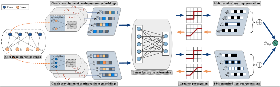
Figure 2. Illustration of L²Q-GCN framwork (Best view in color).

3.2. Basic Implementation: L²Q-GCN_end

The general idea of L²Q-GCN is to learn node representations by propagating latent features via the graph topology (Wu et al., 2019; He et al., 2020; Kipf and Welling, 2017). It performs iterative graph convolution, i.e., propagating and aggregating information of neighbors to update representations (embeddings) of target nodes, which can be formulated as follows:

(1) $$\boldsymbol{v}_{x}^{(l)}=AGG\left(\{\boldsymbol{v}_{y}^{(l-1)}:y\in\mathcal{N}(x)\}\right),$$

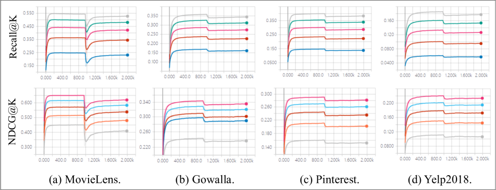
Figure 2. Complete performance curves with annealing tranining strategy.

where $\boldsymbol{v}_{x}^{(l)}$ denotes node $x$’s embedding after $l$ layers of information propagation. $\mathcal{N}(x)$ represents $x$’s neighbor set and $AGG$ is the aggregation function aiming to transform the center node feature and the neighbor features. We illustrate the framework in Figure 2.

3.2.1. Quantization-based Graph Convolution.

We adopt the graph convolution paradigm working on the continuous space from (He et al., 2020) that recently shows good performance under recommendation scenarios. Let $\boldsymbol{v}^{(l)}_{u}\in\mathbb{R}^{c}$ and $\boldsymbol{v}^{(l)}_{i}\in\mathbb{R}^{c}$ denote the continuous feature embeddings of user $u$ and item $i$ computed in the $l$-th layer. They can be respectively updated by utilizing information from the ($l-1$)-th layer in iteration as follows:

(2)

After getting the intermediate embeddings, e.g., $\boldsymbol{v}^{(l)}_{u}$, we conduct 1-bit quantization as:

(3) $$\boldsymbol{q}_{u}^{(l)}=\operatorname{sign}\big{(}\boldsymbol{W}^{T}\boldsymbol{v}^{(l)}_{u}\big{)},\ \ \boldsymbol{q}_{i}^{(l)}=\operatorname{sign}\big{(}\boldsymbol{W}^{T}\boldsymbol{v}^{(l)}_{i}\big{)},$$

where $\boldsymbol{W}\in R^{c\times d}$ is a matrix that transforms $\boldsymbol{v}^{(l)}_{u}$ to $d$-dimensional latent space for 1-bit quantization. Function $\operatorname{sign}(\cdot)$ maps floating-point inputs into the discrete binary space, e.g., $\{-1,1\}^{d}$. By doing so, we can obtain the quantized embedding $\boldsymbol{q}_{u}^{(l)}$ whilst retaining the latent user features directly from $\boldsymbol{v}^{(l)}_{u}$. For ease of L²Q-GCN_end’s binarization storage, we can further conduct a numerical translation to these quantized embeddings from $\{-1,1\}^{d}$ to $\{0,1\}^{d}$. After $L$ layers of feature propagation and quantization, we have built the targeted quantized representations $\mathcal{Q}_{u}$ and $\mathcal{Q}_{i}$ as:

(4) $$\mathcal{Q}_{u}=\{\boldsymbol{q}^{(0)}_{u},\boldsymbol{q}^{(1)}_{u},\cdots,\boldsymbol{q}^{(L)}_{u}\},\ \ \mathcal{Q}_{i}=\{\boldsymbol{q}^{(0)}_{i},\boldsymbol{q}^{(1)}_{i},\cdots,\boldsymbol{q}^{(L)}_{i}\}.$$

Both $\mathcal{Q}_{u}$ and $\mathcal{Q}_{i}$ track the intermediate information binarized from full-precision embeddings at different layers. Intuitively, they represent the interactive information that is propagated back and forth between users and items within these layers, simulating the collaborative filtering effect to exhibit in the quantized encodings for recommendation.

3.2.2. Model Prediction.

Based on the quantized representations of users and items, i.e., $\mathcal{Q}_{u}$ and $\mathcal{Q}_{i}$, we predict the matching scores by naturally adopting the inner product as:

(5) $$\hat{y}_{u,i}=f(\mathcal{Q}_{u})^{T}\cdot f(\mathcal{Q}_{i}),$$

where function $f$ abstracts the way to utilize $\mathcal{Q}_{u}$ and $\mathcal{Q}_{i}$. In this paper, we implement $f$ by taking an element-wise summation:

(6) $$f(\mathcal{Q}_{u})=\sum_{l=0}^{L}\boldsymbol{q}^{(l)}_{u},\ \ f(\mathcal{Q}_{i})=\sum_{l=0}^{L}\boldsymbol{q}^{(l)}_{i}.$$

Clarification. In this work, we interpret quantized representations as integers and apply integer arithmetics in computation. As we will show later in experiments, this introduces about 40% of computation acceleration. Certainly, it can be extended to binary arithmetic logics for further optimization, and we leave it for future work.

3.2.3. Model Optimization.

We then introduce our objective and backward-propagation strategy for optimization.

Objective Function. Our objective function consists of two components, i.e., graph reconstruction loss $\mathcal{L}_{rec}$ and BPR loss $\mathcal{L}_{bpr}$. The motivation of such design is basically twofold:

• $\mathcal{L}_{rec}$ reconstructs the observed topology of interaction graphs;

• $\mathcal{L}_{bpr}$ learns the relative rankings of user preferences towards different items.

Concretely, we implement $\mathcal{L}_{rec}$ with the cross-entropy loss:

(7)

where $\sigma$ is the activation function, e.g., Sigmoid. $\mathcal{L}_{rec}$ bases on the full-precision embeddings at the last layer, e.g., $\boldsymbol{v}^{(L)}_{u}$, providing the latest intermediate information for topology reconstruction as much as possible. As for $\mathcal{L}_{bpr}$, we employ Bayesian Personalized Ranking (BPR) loss (Rendle et al., 2012) as follows:

(8) $$\mathcal{L}_{bpr}=-\sum_{u\in\mathcal{U}}\sum_{i\in\mathcal{N}(u)}\sum_{j\notin\mathcal{N}(u)}\ln\sigma(\hat{y}_{u,i}-\hat{y}_{u,j}).$$

$\mathcal{L}_{bpr}$ relies on the quantized node representations, e.g., $\mathcal{Q}_{u}$, to encourage the prediction of an observed interaction to be higher than its unobserved counterparts (He et al., 2020). Finally, our final objective function is defined as:

(9) $$\mathcal{L}=\mathcal{L}_{rec}+\mathcal{L}_{bpr}+\lambda||\Theta||_{2}^{2},$$

where $\Theta$ is the set of trainable parameters and embeddings, and $||\Theta||_{2}^{2}$ is the $L$2-regularizer parameterized by $\lambda$ to avoid over-fitting.

Clarification. Please notice that at the training stage, we usually take the mean value of $f(\mathcal{Q}_{u})$ by shrinking it as $f(\mathcal{Q}_{u})=f(\mathcal{Q}_{u})/(L+1)$ (likewise for $f(\mathcal{Q}_{i})$). Essentially, this useful training strategy (He et al., 2020; Hongwei et al., 2019) reduces the absolute value of predicted scores to a smaller scale, which significantly stabilizes the training process to avoid the undesirable divergence in embedding optimization; but most importantly, it has no effect on the relative rankings of all scores.

Backward-propagation Strategy. Unfortunately, the sign function is not differentiable. This means that the original derivative of the sign function is 0 almost everywhere, making the intermediate gradients accumulated before quantization zeroed here. To avoid this and approximate the gradients for backward propagation, we adopt the Straight-Through Estimator (Bengio et al., 2013) with gradient clipping as:

(10) $$\left\{\begin{aligned} &\boldsymbol{q}^{(l)}_{u}=\operatorname{sign}\big{(}\phi\big{)},&\text{forward propagation}\\ &\frac{\partial\boldsymbol{q}^{(l)}_{u}}{\partial\phi}:=\boldsymbol{1}_{|\phi|\leq 1}.&\text{backward propagation}\end{aligned}\right.$$

Derivative $\boldsymbol{1}_{|\phi|\leq 1}$ can be viewed as passing gradients e.g., $\Delta$, through hard-tanh function (Courbariaux et al., 2016), i.e., $\max(-1,\min(1,\Delta))$. This passes gradients backwards unchanged when the input of sign function, e.g., $\phi$, is within range of {-1, 1}, and cancels the gradient flow otherwise (Alizadeh et al., 2018). We illustrate the process of gradient propagation in Figure 2.

So far, we have already introduced the skeleton of our proposed network that learns the quantized representations $\mathcal{Q}_{u}$ and $\mathcal{Q}_{i}$ via exploring the interaction graph topology. Since it can be trained in an end-to-end manner, we directly name it as L²Q-GCN_end.

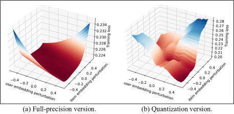
Figure 3. Loss landscapes visualization.

4. Advanced Solution: L²Q-GCN_anl

Although L²Q-GCN_end can achieve the quantization for user-item representations, we argue that there may still exist avenues for further improvement. In this section, we first explain the difficulty of quantization in L²Q-GCN_end, and then give an advanced solution with the annealing training strategy, namely L²Q-GCN_anl, to enhance the recommendation performance.

4.1. Difficulty of Quantization in L²Q-GCN_end

To show it may be challenging to directly quantize L²Q-GCN_end for binary representation, we simulate the optimization trajectories of learnable embeddings and visually compare the loss landscapes of it with its full-precision version (excluding the quantization component) in Figure 3. Concretely, following (Nahshan et al., 2021; Bai et al., 2021), we manually assign perturbations to the learnable user-item embeddings as follows:

(11) $$\boldsymbol{v}_{u}^{(l)}=\boldsymbol{v}_{u}^{(l)}\pm p\cdot\overline{|\boldsymbol{v}_{u}^{(l)}|}\cdot\boldsymbol{1}_{u}^{(l)},\ \ \ \ \boldsymbol{v}_{i}^{(l)}=\boldsymbol{v}_{i}^{(l)}\pm p\cdot\overline{|\boldsymbol{v}_{u}^{(l)}|}\cdot\boldsymbol{1}_{i}^{(l)},$$

where $\overline{|\boldsymbol{v}_{u}^{(l)}|}$ represents the absolute mean value of embedding $\boldsymbol{v}_{u}^{(l)}$ and perturbation magnitudes $p$ are from $\{0.01,0.02,\cdots,0.50\}$. $\boldsymbol{1}_{u}$ is an all-one vector. For each pair of perturbed user-item representations, we plot the loss distribution accordingly.

As we can observe, the full-precision version with no quantization produces a flat and smooth loss surface, showing the local convexity and thus easy to optimize. On the contrary, L²Q-GCN_end has a bumping and complex loss landscape. The steep loss curvature reflects L²Q-GCN_end is more sensitive to perturbation, showing the difficulty in quantization optimization.

4.2. Upgrading in L²Q-GCN_anl

To alleviate the perturbation sensitivity and further improve the model performance, we propose L²Q-GCN_anl.

4.2.1. Quantization with Rescaling Approximation.

Our proposed L²Q-GCN_anl additionally includes layer-wise positive rescaling factors for each node, e.g., $\alpha_{u}^{(l)}\in\mathbb{R}^{+}$, such that $\boldsymbol{v}^{(l)}_{u}\approx$ $\alpha_{u}^{(l)}\boldsymbol{q}^{(l)}_{u}$. In this work, we introduce a simple but effective approach to directly calculate these rescaling factors as:

(12) $$\alpha_{u}^{(l)}=\frac{||\boldsymbol{v}_{u}^{(l)}||_{1}}{d},\ \ \alpha_{i}^{(l)}=\frac{||\boldsymbol{v}_{i}^{(l)}||_{1}}{d}.$$

Instead of setting $\alpha_{u}^{(l)}$ as learnable, such deterministic computation substantially prunes the search space of parameters whilst attaining the approximation functionality. We demonstrate this in Section 5.6.

Based on the quantized user-item representations and the corresponding rescaling factors, we have:

(13)

Consequently, L²Q-GCN_anl approximates $\mathcal{Q}_{u}$ and $\mathcal{Q}_{i}$ by $\mathcal{A}_{u}$ and $\mathcal{A}_{i}$, and updates Equations 5 and 6 for model prediction accordingly.

Space Cost Analysis. The total space cost of L²Q-GCN_end for storing the quantized user-item representations is $O((L+1)Nd)$ (or bits), where $N$ is the number of users and items and $d$ is the dimension of binary embeddings, e.g., $\boldsymbol{v}_{u}^{(l)}$. Furthermore, since L²Q-GCN_anl develops quantization with approximation, supposing that we use 32-bit floating-points for those rescaling factors, the space cost is $O((L+1)N(d+32))$ in total. Compared to the full-precision embedding table at each single one layer, e.g., 32-bit floating-point $\boldsymbol{v}_{u}^{{(l)}}$, $\mathcal{Q}_{u}$ and $\mathcal{Q}_{i}$ have the following theoretical compression ratios:

(14)

Normally, stacking too many layers will cause the over-smoothing problem (Li et al., 2018; Li et al., 2019), incurring performance detriment. Hence, A common setting for $L$ is $L<5$ (He et al., 2020; Wang et al., 2019; Kipf and Welling, 2017; Hamilton et al., 2017), which can still achieve considerable embedding compression.

4.2.2. Annealing Training Strategy.

Another constructive design of L²Q-GCN_anl is the two-step annealing training strategy:

1. we first mask the quantization function and train L²Q-GCN_anl with the full-precision embeddings;

2. when it converges to optimum, we trigger the quantization afterwards to find the targeted quantized representations.

Intuitively, L²Q-GCN_anl moves from a tractable training space to the targeted one for quantization. This can avoid unnecessary exploration towards different optimization directions at the beginning of quantization, guaranteeing the numerical stability in the whole model training. Then at the middle period of training when triggering quantization, as presented in Figure 4, L²Q-GCN_anl firstly meets a performance retracement, but shortly afterwards, it recovers and continues to converge. As we will demonstrate later in experiments, this straightforward but effective strategy can further produce better quantization representations with approximation for Top-K recommendation.

Clarification. we point out that the time cost of training L²Q-GCN_anl shares the same order of magnitude with L²Q-GCN_end. In our implementation, we simply assign half of the total training epochs for the first step and leave the second half for quantization. One may also opt for more flexible strategy to trigger the quantization, e.g., early-stopping, or full-precision version pre-training.

So far, we have introduced all technical details of the proposed L²Q-GCN_end and L²Q-GCN_anl. For the corresponding pseudocodes, please refer to Appendix B. In the following section, we present the experimental results and analysis on our models.

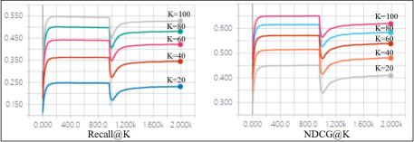
Figure 4. Annealing performance on MovieLens dataset.

5. Experimental Results

We evaluate our model on Top-K recommendation task with the aim of answering the following research questions:

• RQ1. How does L²Q-GCN perform compared to state-of-the-art full-precision and quantization-based recommender models?

• RQ2. How is resource consumption of L²Q-GCN?

• RQ3. How do proposed components of L²Q-GCN_end and L²Q-GCN_anl affect the performance?

5.1. Dataset

• MovieLens is a widely adopted benchmark for movie recommendation. Similar to the setting in (Tan et al., 2020; He et al., 2016; Chen et al., 2021), $y_{u,i}=1$ if user $u$ has an explicit rating score towards item $i$, otherwise $y_{u,i}=0$. In this paper, we use the MovieLens-1M data split.

• Gowalla is the check-in dataset (Liang et al., 2016) collected from Gowalla, where users share their locations by check-in. To guarantee the quality of the dataset, we extract users and items with no less than 10 interactions similar to (Wang et al., 2019; Tan et al., 2020; He et al., 2020).

• Pinterest is an implicit feedback dataset for image recommendation (Geng et al., 2015). Users and images are modeled in a graph. Edges represent the pins over images initiated by users. In this dataset, each user has at least 20 edges. We delete repeated edges between users and images to avoid data leakage in model evaluation.

• Yelp2018 is collected from Yelp Challenge 2018 Edition. In this dataset, local businesses such as restaurants are treated as items. We retain users and items with over 10 interactions similar to (Wang et al., 2019).

Table 1. Datasets.

	# Users	# Items	# Interactions	Density
MovieLens	6,040	3,952	1,000,209	0.04190
Gowalla	29,858	40,981	1,027,370	0.00084
Pinterest	55,186	9,916	1,463,556	0.00267
Yelp2018	31,668	38,048	1,561,406	0.00130

5.2. Competing Methods

We compare our model with two main streams of methods: (1) full-precision recommender systems including CF-based methods (NeurCF), and GCN-based models (NGCF, LightGCN), (2) 1-bit quantization-based models for general item retrieval tasks (LSH, HashNet) and for Top-K recommendation (HashGNN).

• LSH (Gionis et al., 1999) is a classical hashing method. LSH is firstly proposed to approximate the similarity search for massive high-dimensional data and we introduce it for Top-K recommendation by following the adaptation in (Tan et al., 2020).

• HashNet (Cao et al., 2017) is a state-of-the-art deep hashing method that is originally proposed for multimedia retrieval tasks. Similar to (Tan et al., 2020), we adapt it for graph data mainly by replacing the used AlexNet (Krizhevsky et al., 2012) with the general graph convolutional network.

• HashGNN (Tan et al., 2020) is the state-of-the-art 1-bit quantization-based recommender system method with GCN framework. We use HashGNN to denote the vanilla version with hard encoding proposed in (Tan et al., 2020), where each element of quantized user-item embeddings is strictly quantized. We use HashGNN-soft to represent the relaxed version proposed in (Tan et al., 2020), where it adopts a Bernoulli random variable to provide the probability of replacing the quantized digits with continuous values in the original embeddings.

• NeurCF (He et al., 2017) is one state-of-the-art neural network model for collaborative filtering. NeurCF models latent features of users and items to capture their nonlinear feature interactions.

• NGCF (Wang et al., 2019) is one of the state-of-the-art GCN-based recommender models. We compare L${}^{2}Q$-GCN with NGCF mainly to study their performance capabilities in Top-K recommendation.

• LightGCN (He et al., 2020) is the latest state-of-the-art GCN-based recommendation model that has been widely evaluated. We include LightGCN in our experiment mainly to set up the benchmarking as a reference of full-precision recommendation capability.

• Quant-gumbel is a variance of L²Q-GCN with the implementation of Gumbel-softmax for quantization (Jang et al., 2017; Maddison et al., 2017; Zhang and Zhu, 2019). We first expand each embedding bit to a size-two one-hot encoding. Then Quant-gumbel utilizes the Gumbel-softmax trick to replace sign function as relaxation for binary code generation.

Table 2. Performance comparison (underline represents the best performing model; R and D refer to Recall and NDCG).

Model	MovieLens (%)				Gowalla (%)				Pinterest (%)				Yelp2018 (%)
	R@20	R@100	N@20	N@100	R@20	R@100	N@20	N@100	R@20	R@100	N@20	N@100	R@20	R@100	N@20	N@100
LSH	9.35	23.41	13.45	33.49	6.23	15.69	10.23	19.23	6.41	16.55	8.56	15.32	2.73	8.77	4.73	11.63
HashNet	14.98	35.67	23.41	38.14	10.11	24.19	15.31	23.11	8.93	29.43	10.37	21.63	2.64	9.45	6.42	14.68
HashGNN	12.55	34.54	23.63	36.54	9.63	22.13	15.85	24.01	8.01	25.27	10.48	21.19	3.22	10.96	6.62	14.61
HashGNN-soft	18.54	41.83	36.56	55.16	11.49	25.88	17.84	26.53	10.87	34.14	12.35	24.99	4.29	14.03	8.30	17.73
Quant-gumbel	17.48	42.08	34.57	56.50	10.78	26.58	15.62	25.08	9.78	30.63	11.15	22.92	3.91	13.00	8.07	17.08
NeurCF	19.43	48.04	36.85	51.71	13.95	32.76	22.21	27.39	9.09	29.52	13.55	22.24	3.12	10.97	6.45	14.91
NGCF	24.35	54.92	37.30	53.64	15.53	33.32	23.21	28.44	14.30	39.74	13.01	27.06	5.45	15.32	8.73	19.33
LightGCN	25.01	55.71	44.73	65.09	17.80	37.02	24.76	34.91	14.78	39.98	15.91	28.93	6.11	18.05	10.95	21.59
L2Q-GCNend	20.52	49.27	38.41	60.03	14.62	32.24	21.24	30.97	12.52	35.67	13.92	26.37	5.10	16.31	9.62	19.88
% Capacity	82.05%	88.44%	85.87%	92.23%	82.13%	87.10%	85.78%	88.71%	84.71%	89.22%	87.49%	91.15%	83.47%	90.36%	87.85%	92.08%
L2Q-GCNanl	22.81	51.96	42.44	62.96	16.12	34.39	23.62	33.52	13.87	38.25	15.31	28.13	5.74	17.63	10.67	21.32
% Capacity	91.20%	93.27%	94.88%	96.73%	90.56%	92.90%	95.40%	96.02%	93.84%	95.67%	96.23%	97.23%	93.94%	97.67%	97.44%	98.75%

5.3. Experiment Setup

In the evaluation of Top-K recommendation, we apply the learned user-item representations to rank $K$ items for each user with the highest predicted scores, i.e., $\hat{y}_{u,i}$. We choose two widely-used evaluation protocols Recall@$K$ and NDCG@$K$ to evaluate Top-K recommendation capability.

We implement L²Q-GCN model under Python 3.7 and PyTorch 1.14.0 with non-distributed training. The experiments are run on a Linux machine with 4 NVIDIA V100 GPU, 4 Intel Core i7-8700 CPUs, 32 GB of RAM with 3.20GHz. For all the baselines, we follow the official hyper-parameter settings from original papers or as default in corresponding codes. For methods lacking recommended settings, we apply a grid search for hyper-parameters. The embedding dimension is searched in {$32,64,128,256,512$}. The learning rate $\eta$ is tuned within {$10^{-3},5\times 10^{-3},10^{-2},5\times 10^{-2}$} and the coefficient of $L2$ normalization $\lambda$ is tuned among {$10^{-5},10^{-4},10^{-3}$}. We initialize and optimize all models with default normal initializer and Adam optimizer (Kingma and Ba, 2015). To guarantee reproducibility, we report all the hyper-parameter settings in Appendix C.

5.4. Performance Analysis (RQ1)

In this section, we present a comprehensive performance analysis between L${}^{2}Q$-GCN with two layers and competing recommender models of full-precision-based and quantization-based. We evaluate Top-K recommendation over four datasets by varying K in {20, 40, 60, 80, 100}. To achieve a more detailed performance comparison, we summarize the results of Top@20 and Top@100 recommendation in Table 2. We also curve their complete results of Recall@K and NDCG@K metrics and attach them in Appendix D. Generally, L${}^{2}Q$-GCN has made great improvements over quantization-based models and shows the competitive performance compared to full-precision models. We have the following observations:

• The results demonstrate the superiority of L${}^{2}Q$-GCN over all quantization-based models. (1) As shown in Table 2, the state-of-the-art quantization-based GCN model, i.e., HashGNN (and HashGNN-soft), works better than traditional quantization-based baselines, e.g., LSH, HashNet. This shows the effectiveness of graph convolutional architecture in capturing latent information within interaction graphs for quantization preparation and indicates that a direct adaptation of conventional quantization methods may not well handle the Top-K recommendation task.
  (2) Furthermore, thanks to our proposed quantization-based graph convolution design, both L${}^{2}Q$-GCN_end and L${}^{2}Q$-GCN_anl consistently outperform HashGNN and its relaxed version HashGNN-soft. The main reason is that, our topology-aware quantization significantly enriches the user-item representations and alleviates the feature smoothing issue caused by the numerical quantization. We conduct the ablation study on this in the later section.

• Compared to full-precision models, L${}^{2}Q$-GCN presents a competitive performance recovery. (1) L${}^{2}Q$-GCN_end shows the performance superiority over traditional collaborative filtering model, i.e., NeurCF. Considering the large improvement of two GCN-based models, i.e., NGCF and LightGCN, against NeurCF, we can infer the performance gap between L${}^{2}Q$-GCN_end and NeurCF mainly comes from the proposed quantization-based graph convolution. (2) Compared to the best model LightGCN, taking Recall metric as an example, L${}^{2}Q$-GCN_end shows about $82$$\sim$$85\%$ and $87$$\sim$$90\%$ performance capacity in terms of Top@20 and Top@100. This indicates that, as the value of K increases, L${}^{2}Q$-GCN_end can further improve the recommendation accuracy and narrow the gap to LightGCN. (3) Moreover, by utilizing the quantization approximation and annealing training strategy, L${}^{2}Q$-GCN_anl can achieve better performance than NGCF on Gowalla and Yelp2018 datasets. Compared to our basic implementation L${}^{2}Q$-GCN_end, L${}^{2}Q$-GCN_anl further improves the performance recovery by $8$$\sim$$10\%$ and $9$$\sim$$10\%$ in terms of Recall@20 and Recall@100 across all benchmarks, proving the effectiveness of our proposed modification in L${}^{2}Q$-GCN_anl. (4) In addition, with K increasing up to 100, L${}^{2}Q$-GCN_anl presents a similar trend with L${}^{2}Q$-GCN_end such that it performs even closely to LightGCN, i.e., $93$$\sim$$98\%$ and $96$$\sim$$99\%$ in terms of Recall and NDCG, respectively. In a nutshell, the prediction capability of both L${}^{2}Q$-GCN_end and L${}^{2}Q$-GCN_anl develops from fine-grained ranking tasks to coarse-grained ones, e.g., Top-20 to Top-100 recommendation.

• Both L${}^{2}Q$-GCN_end and L${}^{2}Q$-GCN_anl show the deployment flexibility towards different application scenarios. In the pipeline of industrial recommender systems, recall and re-ranking are two important stages that substantially influence recommendation quality. Recall refers to the process of quickly retrieving candidate items from the whole item pool that a given user may interest. Based on the more complex scoring algorithms, re-ranking outputs a precise ranking list of candidate items.

  On the one hand, as we will show later, L${}^{2}Q$-GCN_end can speed up about 40% for candidate generation. Considering its performance improvement on coarse-grained ranking tasks, e.g., Top-100 recommendation, L${}^{2}Q$-GCN_end actually provides an alternative option to accelerate the recall stage. On the other hand, L${}^{2}Q$-GCN_anl further optimizes the recommendation accuracy that performs similarly to LightGCN. Since L${}^{2}Q$-GCN_anl reduces the embedding storage cost to about 9$\times$, we can treat L${}^{2}Q$-GCN_anl as a substitute for the best model, i.e., LightGCN, as a trade-off between space cost and prediction accuracy. We report the details of space and time cost for embedding storage and online inference in the following section.

5.5. Resource Consumption Analysis (RQ2)

In this section, we study the resource consumption in embedding storage and inference time cost. We compare our models with the state-all-the-art full-precision model and quantization-based model, i.e., LightGCN and HashGNN. We take their two-layer structures with the same 128-dimensional embeddings as reference and illustrate with the largest dataset, i.e., Yelp2018, in Figure 5(a). Observations in this section can be popularized to other three datasets and we report the complete results in Appendix D.

Embedding storage compression. Quantized embeddings can largely reduce the space consumption for offline disk storage. To measure the embedding size, we save these embeddings to the disk such that they can recover the well-trained user-item representations for inference. As we can observe, after the binarization for user-item embeddings, L²Q-GCN_end and L²Q-GCN_anl can achieve the space reduction with a factor of about 11$\times$ and 9$\times$, respectively. This basically follows the theoretical bounds that are computed in Equation 14, i.e., $ratio_{end}$ and $ratio_{anl}$ when $L=2$. Furthermore, considering the performance improvement, the space usage of approximation factors of L²Q-GCN_anl is actually acceptable, which may dispel the concerns of large additional storage overhead.

Online inference acceleration. We evaluate the time cost including the score estimation and sorting. L²Q-GCN predicts the scores between users and items by conducting embedding multiplications. At the stage of online inference, we first interpret these binary embeddings by signed integers, e.g., int8, and then conduct integer arithmetics including integer summations and matrix multiplications. Please notice that we leave the development of bitwise operations for online inference for future work. To give a fair comparison on the inference time cost, we disable all arithmetic optimization such as BLAS, MKL, and conduct the experiments using the vanilla NumPy provided by . As shown in Figure 5(a), purely based on the quantized embeddings, L²Q-GCN_end can achieve 39.83% (118.23$\rightarrow$196.49) of inference acceleration. L²Q-GCN_anl takes a similar running time with LightGCN as it introduces the approximation factors in score estimation. Furthermore, Figure 5(b) visualizes the overall evaluation in terms of resource consumption and recommendation accuracy. As the cube’s front-high corner means the ideal optimal performance, our proposed methods make a good balance w.r.t consumption and accuracy.

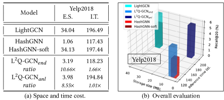
Figure 5. Results of two-layer networks with 128-dimension embeddings (E.S. and I.T. are the abbreviations of embedding size (MB) and inference time (s). Best view in color).

5.6. Ablation Study of L²Q-GCN Model (RQ3)

We evaluate the necessity of each model component in both L²Q-GCN_end and L²Q-GCN_anl. Due to the page limits, we report the Top-20 recommendation results as a reference in Table 3.

5.6.1. Effect of Topology-aware Quantization.

To substantiate the impact of topology-aware quantization in graph convolution, we give a variant of L²Q-GCN_end, i.e., w/o TQ, by disabling the layer-wise quantization and setting it as the final encoder of full-precision graph convolution. As we can observe in Table 3, variant w/o TQ remarkably underperforms L²Q-GCN_end. This demonstrates that simply using the latest-updated embeddings from the GCN framework may not sufficiently model the unique latent features of both users and items, especially for the quantization-based ranking. Via capturing the intermediate information for representation enrichment, our topology-aware quantization can effectively alleviate the ranking smoothness issue caused by the limited expressivity of discrete embeddings. This helps to make the quantized representations of both users and items more discriminative, which leads to the performance improvement on Top-K recommendation.

5.6.2. Effect of Multi-loss in Optimization.

To study the effect of BPR loss $\mathcal{L}_{bpr}$ and graph reconstruction loss $\mathcal{L}_{rec}$, we set two variants, termed by w/o $\mathcal{L}_{bpr}$ and w/o $\mathcal{L}_{rec}$, to optimize L²Q-GCN_end separately. As shown in Table 3, with all other model components, partially using one of $\mathcal{L}_{bpr}$ and $\mathcal{L}_{rec}$ produces large performance decay to L²Q-GCN_end. This confirms the effectiveness of our proposed muti-loss design: while $\mathcal{L}_{bpr}$ assigns higher prediction values to observed interactions, 1.e., $y_{u,i}=1$, than the unobserved user-item pairs, $\mathcal{L}_{rec}$ transfers the graph reconstruction problem to a classification task by using the full-precision embeddings in training. By collectively optimizing these two loss functions, L²Q-GCN_end can learn precise intermediate embeddings from $\mathcal{L}_{rec}$, and produce quantized representations with high-quality relative order information regularized by $\mathcal{L}_{bpr}$ accordingly.

5.6.3. Effect of Rescaling Approximation.

We now discuss the effect of approximation factors in L²Q-GCN_anl. We create two variants, namely w/o RAF and w/in LF. w/o RAF directly removes the rescaling approximation factors and w/in LF means replacing our original approximation factors with learnable ones. We optimize both variants w/o RAF and w/in LF with the annealing training strategy. (1) The performance decline of w/o RAF proves the effectiveness of rescaling approximation for user-item representations. Although these factors are directly calculated and may not be theoretically optimal, they reflect the numerical uniqueness of embeddings for both users and items, which substantially improves L²Q-GCN_anl’s prediction capability. (2) As for w/in LF, the design of learnable rescaling factors does not achieve good performance as expected. One explanation is that, our proposed model currently does not post a direct mathematical constraint to learnable factors ($lf$), e.g., $lf_{u}^{(l)}=\operatorname{argmin}(\boldsymbol{v}^{(l)}_{u}$, $lf_{u}^{(l)}\boldsymbol{q}^{(l)}_{u})$, mainly because they have different embedding dimensionality. This means that purely relying on the stochastic optimization may hardly reach the optimum. In a word, considering the additional search space introduced by this regularization term, we argue that our deterministic rescaling method is simple but effective in practice.

Table 3. Ablation study.

Variant	MovieLens		Gowalla		Pinterest		Yelp2018
	R@20	N@20	R@20	N@20	R@20	N@20	R@20	N@20
L2Q-GCNenl
w/o TQ	17.73	35.31	11.63	15.58	10.29	11.60	4.33	8.58
	-13.60%	-8.07%	-20.45%	-26.65%	-17.81%	-16.67%	-15.10%	-10.81%
w/o $\mathcal{L}_{bpr}$	19.67	37.22	8.66	13.33	5.12	6.01	3.52	7.33
	-4.14%	-3.10%	-40.77%	-37.24%	-59.11%	-56.82%	-30.98%	-23.80%
w/o $\mathcal{L}_{rec}$	16.98	32.76	8.32	9.28	10.86	11.55	3.33	6.60
	-17.25%	-14.71%	-43.09%	-56.31%	-13.26%	-17.03%	-34.71%	-31.39%
Best	20.52	38.41	14.62	21.24	12.52	13.92	5.10	9.62
L2Q-GCNanl
w/o RAF	20.86	38.14	10.29	12.10	11.19	12.11	4.25	8.09
	-8.55%	-10.13%	-36.17%	-48.77%	-19.32%	-20.90%	-25.96%	-24.18%
w/in LF	20.05	38.25	14.53	21.23	12.35	13.65	5.56	10.20
	-12.10%	-9.87%	-9.86%	-10.12%	-10.96%	-10.84%	-3.13%	-4.40%
w/o AT	21.24	40.05	15.09	22.70	13.37	14.75	5.27	9.96
	-6.88%	-5.63%	-6.39%	-3.90%	-3.60%	-3.66%	-8.19%	-6.65%
Best	22.81	42.44	16.12	23.62	13.87	15.31	5.74	10.67

5.6.4. Effect of Annealing Training Strategy.

We disable the annealing training strategy by only adapting the rescaling approximation design to L²Q-GCN_end and denote the variant as w/o AT. The performance of w/o AT well demonstrate the usefulness of our utilized annealing training strategy in avoiding unnecessary optimization directions and the numerical stability for producing better recommendation accuracy.

In conclusion, the ablation study well justifies the necessity of each model component in both L²Q-GCN_end and L²Q-GCN_anl. We also discuss the effect of different hyperparameter settings, e.g., layer depth $L$, quantization dimension $d$, to model performance and attached the results in Appendix D.

6. Conclusion and Future Work

In this work, we propose L²Q-GCN to study the problem of 1-bit representation quantization for Top-K recommendation. While L²Q-GCN_end implements the basic framework of L²Q-GCN to generate the quantized user-item representations, L²Q-GCN_anl further improves the recommendation capability by attaining 90$\sim$99% performance recovery compared to the state-of-the-art model. The extensive experiments over four real benchmarks not only prove the effectiveness of our proposed models but also justify the necessity of each model component.

As for future work, we point out two possible directions. (1) Instead of relying on integer arithmetics, how to develop the bitwise-operation-supported computation for efficient inference is an important topic to investigate. (2) It is also worth studying the problem of complete network binarization for the GCN framework, as it is more fundamental to many GCN-related methods for model compression and computation acceleration.

Appendix A Notation and Meanings

Table 1 explains all key notations used in this paper.

Appendix B pseudocodes of L²Q-GCN

We attached the detailed pseudocodes of L²Q-GCN_end and L²Q-GCN_anl in Algorithms 1 and 2, respectively.

Appendix C Hyper-parameter Settings

We report all the hyper-parameter settings in Table 2. Please notice that, in table 2, $B$ is the batch size, $\eta$ represents the learning rate, and $\lambda$ is the coefficient of $L$2 normalization.

Appendix D Complete Results

For detailed curves of Top-K recommendation, please refer to Figure 1. For the study of different hyperparameter setttings, i.e., layer depth $L$ and quantization dimension $d$, please refer to Table 4 and Table 5 accordingly.

Table 1. Notations and meanings.

Notation	Meaning
$\mathcal{U}$, $\mathcal{I}$	The sets of users, items.
$y_{u,i}$, $\hat{y}_{u,i}$	$y_{u,i}$$=$$1$ means there is an observed interaction between user $u$ and item $i$, otherwise $y_{u,i}$$=$$0$. $\hat{y}_{u,i}$ is the estimated matching score.
$\boldsymbol{v}_{x}^{(l)}$,	continuous embedding of node $x$ at the $l$-th layer.
$\boldsymbol{q}_{x}^{(l)}$,	binary embedding of node $x$ at the $l$-th layer.
$\mathcal{Q}_{x}$,	quantized representation of node $x$.
$\mathcal{A}_{x}$,	approximation-based quantized representation of node $x$.

Input: Interaction graph $\mathcal{G}$; trainable parameters $\Theta$: $\{\boldsymbol{v}_{u}\}_{u\in\mathcal{U}}$, $\{\boldsymbol{v}_{i}\}_{i\in\mathcal{I}}$, $\boldsymbol{W}$; hyper-parameters: $B$, $d_{end}$, $L$, $\eta$, $\lambda$.

1

Output: Prediction function $\mathcal{F}(u,i|\Theta,\mathcal{G})$

2 $\mathcal{Q}_{u}\leftarrow\emptyset$, $\mathcal{Q}_{i}\leftarrow\emptyset$;

3 while L²Q-GCN_end not converge do

4       for $(u,i)\in\mathcal{G}$ that $y_{u,i}=1$ do

5             for $l=1,\cdots,L$ do

6                   $\boldsymbol{v}_{u}^{(l)}\leftarrow\sum_{i\in\mathcal{N}(u)}\frac{1}{\sqrt{|\mathcal{N}(u)|\cdot|\mathcal{N}(i)|}}v^{(l-1)}_{i}$;

7                   $\boldsymbol{v}_{i}^{(l)}\leftarrow\sum_{u\in\mathcal{N}(i)}\frac{1}{\sqrt{|\mathcal{N}(i)|\cdot|\mathcal{N}(u)|}}v^{(l-1)}_{u}$;

8                   $q_{u}^{(l+1)}\leftarrow\operatorname{sign}\big{(}\boldsymbol{W}^{T}\boldsymbol{v}^{(l)}_{u}\big{)}$; $q_{i}^{(l)}\leftarrow\operatorname{sign}\big{(}\boldsymbol{W}^{T}\boldsymbol{v}^{(l)}_{i}\big{)}$;

9                   Update ($\mathcal{Q}_{u}$, $\mathcal{Q}_{i}$);

10                   $\frac{\partial\boldsymbol{q}^{(l)}_{u}}{\partial\phi},\frac{\partial\boldsymbol{q}^{(l)}_{i}}{\partial\phi}\leftarrow\boldsymbol{1}_{|\phi|\leq 1}$ for backforward propagation;

11                  

12            Update ($\mathcal{Q}_{u}$, $\mathcal{Q}_{i}$) with $q_{u}^{(0)},q_{i}^{(0)}$;

13             $\mathcal{L}\leftarrow$ compute loss and optimize L²Q-GCN_end model;

14            

15      

16return $\mathcal{F}$.

Algorithm 1 L²Q-GCN_end algorithm

Table 2. Hyper-parameter settings for the four datasets.

	MovieLens	Gowalla	Pinterest	Yelp2018
$B$	2048	2048	2048	2048
$d_{end}$	256	64	64	64
$d_{anl}$	256	256	128	256
$\eta$	$1\times 10^{-3}$	$1\times 10^{-3}$	$1\times 10^{-3}$	$1\times 10^{-3}$
$\lambda$	$1\times 10^{-4}$	$1\times 10^{-4}$	$1\times 10^{-4}$	$1\times 10^{-4}$

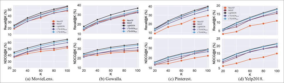
Figure 1. topk.

Table 3. Space and time results of two-layer networks with 128-dimension embeddings.

Model	MovieLens		Gowalla		Pinterest		Yelp2018
	E.S.	I.T.	E.S.	I.T.	E.S.	I.T.	E.S.	I.T.
LightGCN	4.88	3.42	34.59	190.41	28.45	82.66	34.04	196.49
L2Q-GCNend	0.47	2.19	3.24	118.97	2.98	53.48	3.19	118.23
Gap	10.38$\times$	1.56$\times$	10.68$\times$	1.60$\times$	9.55$\times$	1.55$\times$	10.66$\times$	1.66$\times$
L2Q-GCNanl	0.58	3.55	4.05	191.32	3.73	81.77	3.98	194.84
Gap	8.41$\times$	0.96$\times$	8.54$\times$	1.00$\times$	7.63$\times$	1.01$\times$	8.55$\times$	1.01$\times$

Table 4. Top-20 recommendation (%) w.r.t different $L$.

$L$	MovieLens		Gowalla		Pinterest		Yelp2018
	R@20	N@20	R@20	N@20	R@20	N@20	R@20	N@20
L2Q-GCNenl
$L=1$	20.81	39.08	13.59	19.86	11.34	12.79	4.76	9.28
$L=2$	20.52	38.41	14.62	21.24	12.52	13.92	5.10	9.62
$L=3$	10.57	33.44	12.65	19.23	6.41	7.39	3.83	7.95
$L=4$	6.32	19.25	13.85	20.26	3.56	4.51	4.65	9.03
L2Q-GCNanl
$L=1$	20.56	39.51	15.82	23.04	13.11	14.50	5.52	10.31
$L=2$	22.81	42.44	16.12	23.62	13.87	15.31	5.74	10.67
$L=3$	21.93	40.85	14.60	22.22	12.90	14.52	5.35	10.14
$L=4$	21.72	40.46	14.63	22.24	11.31	13.16	4.96	9.74

Table 5. Top-20 recommendation (%) w.r.t different $d$.

$L$	MovieLens		Gowalla		Pinterest		Yelp2018
	R@20	N@20	R@20	N@20	R@20	N@20	R@20	N@20
L2Q-GCNenl
$d=64$	16.65	28.23	14.62	21.24	9.63	9.69	5.10	9.62
$d=128$	18.02	33.15	14.41	19.91	12.52	13.92	4.86	9.63
$d=256$	20.52	38.41	10.39	14.29	10.37	11.62	4.26	8.55
$d=512$	17.79	31.49	13.23	20.65	10.22	11.38	3.49	7.43
L2Q-GCNanl
$d=64$	20.02	38.89	14.29	21.35	11.85	12.76	4.21	8.42
$d=128$	21.64	40.82	15.38	22.84	13.87	15.31	4.94	9.17
$d=256$	22.81	42.44	16.12	23.62	12.63	14.20	5.74	10.67
$d=512$	21.23	40.17	15.54	23.11	12.41	14.04	5.28	9.42

Input: Interaction graph $\mathcal{G}$; trainable parameters $\Theta$: $\{\boldsymbol{v}_{u}\}_{u\in\mathcal{U}}$, $\{\boldsymbol{v}_{i}\}_{i\in\mathcal{I}}$, $\boldsymbol{W}$; hyper-parameters: $B$, $d_{end}$, $L$, $\eta$, $\lambda$.

1

Output: Prediction function $\mathcal{F}(u,i|\Theta,\mathcal{G})$

2 $\mathcal{Q}_{u}\leftarrow\emptyset$, $\mathcal{Q}_{i}\leftarrow\emptyset$;

3 while L²Q-GCN_anl not converge do

4       for $(u,i)\in\mathcal{G}$ that $y_{u,i}=1$ do

5             for $l=1,\cdots,L$ do

6                   $\boldsymbol{v}_{u}^{(l)}\leftarrow\sum_{i\in\mathcal{N}(u)}\frac{1}{\sqrt{|\mathcal{N}(u)|\cdot|\mathcal{N}(i)|}}v^{(l-1)}_{i}$;

7                   $\boldsymbol{v}_{i}^{(l)}\leftarrow\sum_{u\in\mathcal{N}(i)}\frac{1}{\sqrt{|\mathcal{N}(i)|\cdot|\mathcal{N}(u)|}}v^{(l-1)}_{u}$;

8                   $q_{u}^{(l)}\leftarrow\big{(}\boldsymbol{W}^{T}\boldsymbol{v}^{(l)}_{u}\big{)}$; $q_{i}^{(l)}\leftarrow\big{(}\boldsymbol{W}^{T}\boldsymbol{v}^{(l)}_{i}\big{)}$;

9                   if with quantization then

10                         $q_{u}^{(l)}\leftarrow\operatorname{sign}\big{(}q_{u}^{(l)})$; $q_{i}^{(l)}\leftarrow\operatorname{sign}\big{(}q_{i}^{(l)})$;

11                         Setting gradients for backforward propagation;

12                        

13                  $\alpha_{u}^{(l)}\leftarrow\frac{||\boldsymbol{v}_{u}^{(l)}||_{1}}{d}$, $\alpha_{u}^{(l)}\leftarrow\frac{||\boldsymbol{v}_{u}^{(l)}||_{1}}{d}$;

14                   Update ($\mathcal{A}_{u}$, $\mathcal{A}_{i}$) with $\alpha_{u}^{(l)}q_{u}^{(l)}$, $\alpha_{i}^{(l)}q_{i}^{(l)}$;

15                  

16            Update ($\mathcal{A}_{u}$, $\mathcal{A}_{i}$) with $\alpha_{u}^{(0)}q_{u}^{(0)},\alpha_{u}^{(0)}q_{i}^{(0)}$;

17             $\mathcal{L}\leftarrow$ compute loss and optimize L²Q-GCN_anl model;

18            

19      

20return $\mathcal{F}$.

Algorithm 2 L²Q-GCN_anl algorithm

References

- (1)
- our ([n.d.]) [n.d.]. Codes and Datasets of L2Q-GCN. https://drive.google.com/file/d/1-9_kP60af0r86dAvIy4mdq_rPkTyCfMA/view?usp=sharing.
- Alizadeh et al. (2018) Milad Alizadeh, Javier Fernández-Marqués, Nicholas D Lane, and Yarin Gal. 2018. An empirical study of binary neural networks’ optimisation. In ICLR.
- Bahri et al. (2021) Mehdi Bahri, Gaétan Bahl, and Stefanos Zafeiriou. 2021. Binary Graph Neural Networks. In CVPR. 9492–9501.
- Bai et al. (2021) Haoli Bai, Wei Zhang, Lu Hou, Lifeng Shang, Jing Jin, Xin Jiang, Qun Liu, Michael Lyu, and Irwin King. 2021. Pushing the limit of bert quantization. (2021).
- Bengio et al. (2013) Yoshua Bengio, Nicholas Léonard, and Aaron Courville. 2013. Estimating or propagating gradients through stochastic neurons for conditional computation. arXiv (2013).
- Bennett (1948) William Ralph Bennett. 1948. Spectra of quantized signals. The Bell System Technical Journal 27, 3 (1948), 446–472.
- Berg et al. (2017) Rianne van den Berg, Thomas N Kipf, and Max Welling. 2017. Graph convolutional matrix completion. arXiv (2017).
- Cao et al. (2017) Zhangjie Cao, Mingsheng Long, Jianmin Wang, and Philip S Yu. 2017. Hashnet: Deep learning to hash by continuation. In ICCV. 5608–5617.
- Chen et al. (2021) Yankai Chen, Menglin Yang, Yingxue Zhang, Mengchen Zhao, Ziqiao Meng, Jianye Hao, and Irwin King. 2021. Modeling Scale-free Graphs with Hyperbolic Geometry for Knowledge-aware Recommendation. arXiv (2021).
- Cheng et al. (2018) Zhiyong Cheng, Ying Ding, Lei Zhu, and Mohan Kankanhalli. 2018. Aspect-aware latent factor model: Rating prediction with ratings and reviews. In WWW. 639–648.
- Courbariaux et al. (2016) Matthieu Courbariaux, Itay Hubara, Daniel Soudry, Ran El-Yaniv, and Yoshua Bengio. 2016. Binarized neural networks: Training deep neural networks with weights and activations constrained to+ 1 or-1. arXiv (2016).
- Covington et al. (2016) Paul Covington, Jay Adams, and Emre Sargin. 2016. Deep neural networks for youtube recommendations. In Recsys. 191–198.
- Erin Liong et al. (2015) Venice Erin Liong, Jiwen Lu, Gang Wang, Pierre Moulin, and Jie Zhou. 2015. Deep hashing for compact binary codes learning. In CVPR. 2475–2483.
- Geng et al. (2015) Xue Geng, Hanwang Zhang, Jingwen Bian, and Tat-Seng Chua. 2015. Learning image and user features for recommendation in social networks. In ICCV. 4274–4282.
- Gersho and Gray (2012) Allen Gersho and Robert M Gray. 2012. Vector quantization and signal compression. Vol. 159. Springer Science & Business Media.
- Gionis et al. (1999) Aristides Gionis, Piotr Indyk, Rajeev Motwani, et al. 1999. Similarity search in high dimensions via hashing. In Vldb, Vol. 99. 518–529.
- Hamilton et al. (2017) William L Hamilton, Rex Ying, and Jure Leskovec. 2017. Inductive representation learning on large graphs. In NeurIPS. 1025–1035.
- He et al. (2020) Xiangnan He, Kuan Deng, Xiang Wang, Yan Li, Yongdong Zhang, and Meng Wang. 2020. Lightgcn: Simplifying and powering graph convolution network for recommendation. In SIGIR. 639–648.
- He et al. (2017) Xiangnan He, Lizi Liao, Hanwang Zhang, Liqiang Nie, Xia Hu, and Tat-Seng Chua. 2017. Neural collaborative filtering. In WWW. 173–182.
- He et al. (2016) Xiangnan He, Hanwang Zhang, Min-Yen Kan, and Tat-Seng Chua. 2016. Fast matrix factorization for online recommendation with implicit feedback. In SIGIR. 549–558.
- Hongwei et al. (2019) Wang Hongwei, Zhao Miao, Xie Xing, Li Wenjie, and Guo Minyi. 2019. Knowledge Graph Convolutional Networks for Recommender Systems. (2019), 3307–3313.
- Hubara et al. (2016) Itay Hubara, Matthieu Courbariaux, Daniel Soudry, Ran El-Yaniv, and Yoshua Bengio. 2016. Binarized neural networks. NeurIPS 29 (2016).
- Jang et al. (2017) Eric Jang, Shixiang Gu, and Ben Poole. 2017. Categorical reparameterization with gumbel-softmax. (2017).
- Kang et al. (2021) Wang-Cheng Kang, Derek Zhiyuan Cheng, Tiansheng Yao, Xinyang Yi, Ting Chen, Lichan Hong, and Ed H Chi. 2021. Learning to Embed Categorical Features without Embedding Tables for Recommendation. In SIGKDD. 840–850.
- Kingma and Ba (2015) Diederik P Kingma and Jimmy Ba. 2015. Adam: A method for stochastic optimization. (2015).
- Kipf and Welling (2017) Thomas N Kipf and Max Welling. 2017. Semi-supervised classification with graph convolutional networks. (2017).
- Krizhevsky et al. (2012) Alex Krizhevsky, Ilya Sutskever, and Geoffrey E Hinton. 2012. Imagenet classification with deep convolutional neural networks. NeurIPS 25 (2012), 1097–1105.
- Li et al. (2019) Guohao Li, Matthias Muller, Ali Thabet, and Bernard Ghanem. 2019. Deepgcns: Can gcns go as deep as cnns?. In ICCV. 9267–9276.
- Li et al. (2018) Qimai Li, Zhichao Han, and Xiao-Ming Wu. 2018. Deeper insights into graph convolutional networks for semi-supervised learning. In AAAI.
- Liang et al. (2016) Dawen Liang, Laurent Charlin, James McInerney, and David M Blei. 2016. Modeling user exposure in recommendation. In WWW. 951–961.
- Lin et al. (2017) Xiaofan Lin, Cong Zhao, and Wei Pan. 2017. Towards accurate binary convolutional neural network. (2017).
- Maddison et al. (2017) Chris J Maddison, Andriy Mnih, and Yee Whye Teh. 2017. The concrete distribution: A continuous relaxation of discrete random variables. (2017).
- Nahshan et al. (2021) Yury Nahshan, Brian Chmiel, Chaim Baskin, Evgenii Zheltonozhskii, Ron Banner, Alex M Bronstein, and Avi Mendelson. 2021. Loss aware post-training quantization. Machine Learning (2021), 1–18.
- Qin et al. (2020) Haotong Qin, Ruihao Gong, Xianglong Liu, Mingzhu Shen, Ziran Wei, Fengwei Yu, and Jingkuan Song. 2020. Forward and backward information retention for accurate binary neural networks. In CVPR. 2250–2259.
- Rastegari et al. (2016) Mohammad Rastegari, Vicente Ordonez, Joseph Redmon, and Ali Farhadi. 2016. Xnor-net: Imagenet classification using binary convolutional neural networks. In ECCV. Springer, 525–542.
- Rendle et al. (2012) Steffen Rendle, Christoph Freudenthaler, Zeno Gantner, and Lars Schmidt-Thieme. 2012. BPR: Bayesian personalized ranking from implicit feedback. arXiv (2012).
- Shi et al. (2020) Hao-Jun Michael Shi, Dheevatsa Mudigere, Maxim Naumov, and Jiyan Yang. 2020. Compositional embeddings using complementary partitions for memory-efficient recommendation systems. In SIGKDD. 165–175.
- Sun et al. (2019) Jianing Sun, Yingxue Zhang, Chen Ma, Mark Coates, Huifeng Guo, Ruiming Tang, and Xiuqiang He. 2019. Multi-graph convolution collaborative filtering. In ICDM. IEEE, 1306–1311.
- Tailor et al. (2021) Shyam A Tailor, Javier Fernandez-Marques, and Nicholas D Lane. 2021. Degree-quant: Quantization-aware training for graph neural networks. 9th ICLR (2021).
- Tan et al. (2020) Qiaoyu Tan, Ninghao Liu, Xing Zhao, Hongxia Yang, Jingren Zhou, and Xia Hu. 2020. Learning to hash with graph neural networks for recommender systems. In WWW. 1988–1998.
- Wang et al. (2021) Junfu Wang, Yunhong Wang, Zhen Yang, Liang Yang, and Yuanfang Guo. 2021. Bi-gcn: Binary graph convolutional network. In CVPR. 1561–1570.
- Wang et al. (2017) Jingdong Wang, Ting Zhang, Nicu Sebe, Heng Tao Shen, et al. 2017. A survey on learning to hash. TPAMI 40, 4 (2017), 769–790.
- Wang et al. (2019) Xiang Wang, Xiangnan He, Meng Wang, Fuli Feng, and Tat-Seng Chua. 2019. Neural graph collaborative filtering. In SIGIR. 165–174.
- Wu et al. (2019) Felix Wu, Amauri Souza, Tianyi Zhang, Christopher Fifty, Tao Yu, and Kilian Weinberger. 2019. Simplifying graph convolutional networks. In ICML. PMLR, 6861–6871.
- Wu et al. (2021) Wei Wu, Bin Li, Chuan Luo, and Wolfgang Nejdl. 2021. Hashing-Accelerated Graph Neural Networks for Link Prediction. In WWW. 2910–2920.
- Xu et al. (2020) Yang Xu, Lei Zhu, Zhiyong Cheng, Jingjing Li, and Jiande Sun. 2020. Multi-feature discrete collaborative filtering for fast cold-start recommendation. In AAAI, Vol. 34. 270–278.
- Ying et al. (2018) Rex Ying, Ruining He, Kaifeng Chen, Pong Eksombatchai, William L Hamilton, and Jure Leskovec. 2018. Graph convolutional neural networks for web-scale recommender systems. In SIGKDD. 974–983.
- Zhang et al. (2016) Hanwang Zhang, Fumin Shen, Wei Liu, Xiangnan He, Huanbo Luan, and Tat-Seng Chua. 2016. Discrete collaborative filtering. In SIGIR. 325–334.
- Zhang et al. (2017) Yan Zhang, Defu Lian, and Guowu Yang. 2017. Discrete personalized ranking for fast collaborative filtering from implicit feedback. In AAAI, Vol. 31.
- Zhang et al. (2019) Yingxue Zhang, Soumyasundar Pal, Mark Coates, and Deniz Ustebay. 2019. Bayesian graph convolutional neural networks for semi-supervised classification. In AAAI, Vol. 33. 5829–5836.
- Zhang and Zhu (2019) Yifei Zhang and Hao Zhu. 2019. Doc2hash: Learning discrete latent variables for documents retrieval. In ACL. 2235–2240.
- Zhu et al. (2016) Han Zhu, Mingsheng Long, Jianmin Wang, and Yue Cao. 2016. Deep hashing network for efficient similarity retrieval. In AAAI, Vol. 30.