[datatype=bibtex] [overwrite] [fieldsource=doi, final] [fieldset=url, null] [fieldset=eprint, null]

SupplementalMaterials

Bio-inspired Polarization Event Camera

1 Abstract

The stomatopod (mantis shrimp) visual system  [1, 2, 3] has recently provided a blueprint for the design of paradigm-shifting polarization and multispectral imaging sensors  [4, 5, 6, 7, 8, 36, 10], enabling solutions to challenging medical [8, 36] and remote sensing problems [11]. However, these bioinspired sensors lack the high dynamic range (HDR) and asynchronous polarization vision capabilities of the stomatopod visual system, limiting temporal resolution to $\sim$12 ms and dynamic range to $\sim$72 dB. Here we present a novel stomatopod-inspired polarization camera which mimics the sustained and transient biological visual pathways to save power and sample data beyond the maximum Nyquist frame rate. This bio-inspired sensor simultaneously captures both synchronous intensity frames and asynchronous polarization brightness change information with sub-millisecond latencies over a million-fold range of illumination. Our PDAVISPolarization Dynamic and Active pixel VIsion Sensor camera is comprised of 346x260 pixels, organized in 2-by-2 macropixels, which filter the incoming light with four linear polarization filters offset by 45°. Polarization information is reconstructed using both low cost and latency event-based algorithms and more accurate but slower deep neural networks. Our sensor is used to image HDRhigh dynamic range polarization scenes which vary at high speeds and to observe dynamical properties of single collagen fibers in bovine tendon under rapid cyclical loads.

2 Main

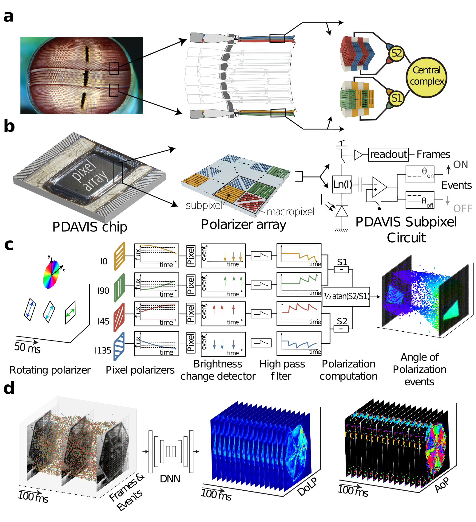
Figure 1: Overview of our bio-inspired polarization vision sensor. a, Polarization vision in the mantis shrimp eye (left) is in part enabled by two sets of orthogonal microvilli located in the dorsal and ventral hemisphere (center), capturing total of 4 linear polarization states offset by 45 degrees (right). This polarization sensitivity paired with logarithmic photoreceptors that output only brightness change enable the mantis shrimp to be effective predator in the shallow coral reefs [2]. b, The PDAVISPolarization Dynamic and Active pixel VIsion Sensor polarization event camera (left), effectively mimics the mantis shrimp eye by integrating an array of pixelated polarization filters offset by 45 degrees (center, angle indicated by false colors) with a vision sensor that provides both sustained pathway frames and transient pathway log-scale brightness change events (right) (see Supplementary Material 1). c, A rectangular rotating linear polarizer (left) generates a stream of brightness change events from the four subpixels in the PDAVISPolarization Dynamic and Active pixel VIsion Sensor macropixels that see the polarizer (center). A temporal filter approximates the temporal derivative from the four individual pixels and then computes the AoPAngle of Polarization. The result is a stream of AoPAngle of Polarization events with low latency (right). (see Supplementary Material 2). d, A polarization filter wheel is rotated in front of PDAVISPolarization Dynamic and Active pixel VIsion Sensor, which produces frames and events (left) represented in false colors shown in (c). A DNNDeep Neural Network (center-left) reconstructs DoLPDegree of Linear Polarization (center-right) and AoPAngle of Polarization (right) from the brightness change events at a higher rate than the cameras maximum frame rate (see Supplementary Material 2).

Visual information is encoded in light by intensity, color, and polarization [2]. This information is sensed by biological eyes and artificial cameras which each have been optimized by evolution driven by maximum fitness. Eyes have evolved to support visually guided behavior for the benefit of survival, while digital cameras have mainly evolved to supply consumer demand for high-resolution photography. These different evolutionary paths have created very different visual systems. Existing spectral and polarization digital cameras use synchronous and generally redundant frames with linear photo response [36, 5, 12, 13, 14]. By contrast, eyes are asynchronous, have a compressed nonlinear response, and their output is sparse and highly informative [2].

The mantis shrimp visual system (Fig. 1a) is considered one of the most sophisticated visual systems in nature. It is sensitive to more than 12 spectral, 4 linear, and 2 circular polarization channels [1, 2]. Its photosensitive microvilli have a logarithmic HDRhigh dynamic range response to incident light. Sensitivity to linearly polarized light is in part expressed in the dorsal and ventral parts of the ommatidia, where individual photoreceptors are comprised of orthogonal sets of microvilli sensitive to orthogonal polarization states. The dorsal/ventral views largely overlap, and since the dorsal and ventral microvilli are offset by 45°, four linear polarization states offset by 45° are captured by the eye. The logarithmic photo responses of the microvilli enable high dynamic range polarization sensing capabilities, while their asynchronous response to temporally varying brightness greatly reduces the visual information that is transmitted to their brain for further processing. It is believed that mantis shrimp use polarization to discriminate short-range prey [2], to select a mating partner [15] and to orient during short-range navigation using celestial polarization patterns [16].

Our work capitalizes on the development of bioinspired neuromorphic vision sensors, which have enabled higher dynamic range and lower latency machine vision [29, 18]. Inspired by the ommatidia of mantis shrimp, individual PDAVISPolarization Dynamic and Active pixel VIsion Sensor subpixel circuits [29] are each overlaid with one of four pixelated linear polarization filters (Fig. 1b). The PDAVISPolarization Dynamic and Active pixel VIsion Sensor takes inspiration from biology by saving energy by partitioning the perception of fine detail and fast motion into sustained and transient pathways [2]. It provides a relatively low frequency synchronous readout of frames like conventional cameras (the “sustained” pathway), and it concurrently outputs a high frequency stream of asynchronous brightness change events (the “transient” pathway). Each event represents a signed log intensity change. Pixels that see more brightness change generate more events, and the events have sub-millisecond temporal resolution driven by the dynamics of the scene. The events enable reconstructing the absolute intensity between the synchronous frame intensity samples.

3 Reconstructing Polarization Information

Polarization is encoded in the relative responses of the subpixels with the 4 linear polarizers offset by 45°. Absolute intensity is encoded in the sum of crossed polarization subpixel outputs. For a direct comparison with a state-of-the-art commercially available polarization imaging sensor (Sony IMX250 [19]), we processed the PDAVISPolarization Dynamic and Active pixel VIsion Sensor output to extract Angle of Polarization (AoP), the predominant axis of oscillation as light propagates in time and space, and Degree of Linear Polarization (DoLP), the amount of linearly polarized in the incident light. We studied three related algorithms: an economical algorithm processing only events, an economical Complementary Filter (CF) algorithm which fuses frames and events [39], and an expensive Deep Neural Network (DNN) that takes events as input [40] (see Methods, Supplementary Material 2 and Supplementary Table 2). We did four sets of experiments.

First, we assessed the ability to reconstruct the time-varying AoPAngle of Polarization of fully linearly polarized light (with DoLPDegree of Linear Polarization=1) by rotating a linear polarizer at constant speeds (Fig. 2, Supplementary Material 1, Supplementary Figs. S2, Supplementary Video 1). At low rotation speeds of less than 60 RPMRevolutions per Minute, the AoPAngle of Polarization reconstruction error from both sensors is less than 5°, with the Sony sensor having the lowest reconstruction error. The reconstructed DoLPDegree of Linear Polarization is nearly 1 from both sensors, as expected. Since Sony’s polarization sensor is fabricated in an optimized semiconductor fab, the mismatches in both the optical properties of the pixelated polarization filters and electrical properties of the photodiodes and read-out circuits are minimal, resulting in high accuracy in the reconstructed polarization information for slow rotation rate. Our PDAVISPolarization Dynamic and Active pixel VIsion Sensor prototype has larger mismatches between the optical properties of the pixelated filters as well as read-out electronics resulting in larger error at low frequency, which can be mitigated by calibration [22]. However, when the linear polarizer is rotated above $\sim$100 RPM, the Sony and PDAVISPolarization Dynamic and Active pixel VIsion Sensor frames start aliasing and motion blurring (Fig. 2c), which decreases the estimated DoLPDegree of Linear Polarization and increases the AoPAngle of Polarization error. The PDAVISPolarization Dynamic and Active pixel VIsion Sensor events maintain precise timing information and the reconstructions using events have AoPAngle of Polarization and DoLPDegree of Linear Polarization error less than 10° all the way to 1000 RPMRevolutions per Minute.

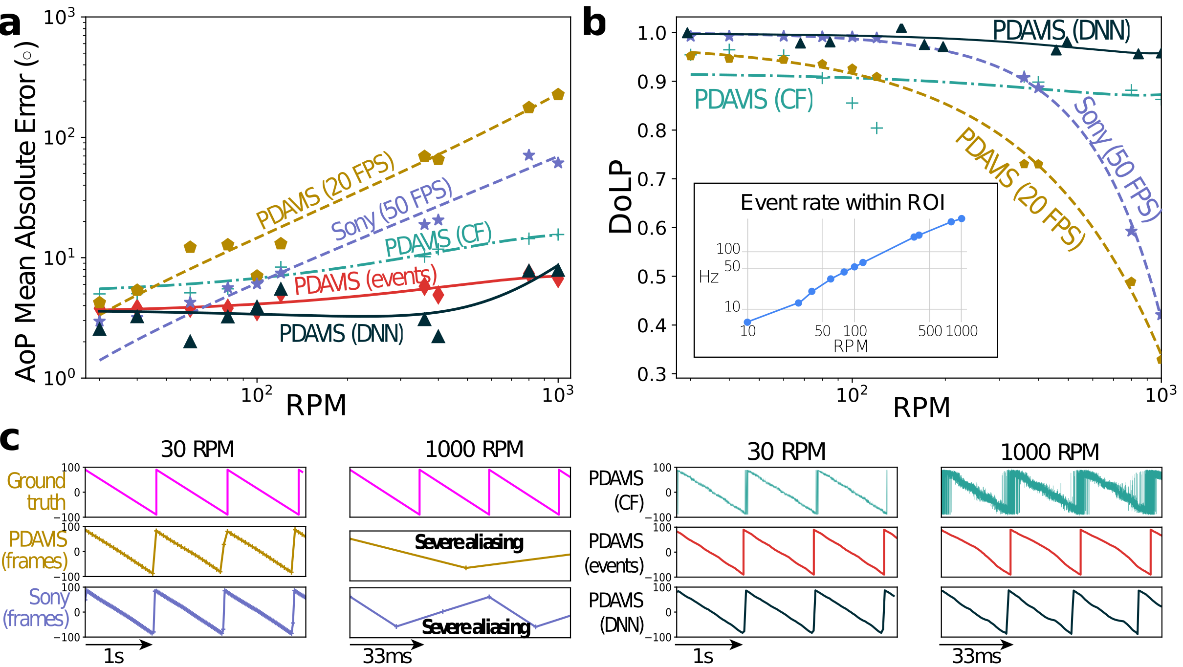
Figure 2: Comparison of frame-based and event-based AoPAngle of Polarization and DoLPDegree of Linear Polarization reconstruction accuracy at various rotational speeds. Input is image of fully linearly polarized light from a rotating linear polarizer. a Mean absolute error (MAE) of AoPAngle of Polarization reconstruction for the various methods averaged over 12x12 ROIRegion of Interest centered on the polarizer. (see Supplementary Material 2). PDAVISPolarization Dynamic and Active pixel VIsion Sensor and Sony frame rates are shown in plots and both exposure durations were fixed to 20 ms. The frames methods use only synchronous intensity frames. The CFComplementary Filter method fuses 20 FPS frames and events using a method adapted from [39]. The events method is illustrated in Fig. 1c. The DNNDeep Neural Network method uses only events together with the convolutional recurrent neural network [40]. b DoLPDegree of Linear Polarization reconstructions. Both CFComplementary Filter or DNNDeep Neural Network methods show that using events allows reconstructing DoLPDegree of Linear Polarization well beyond the limiting Nyquist frequency of the frame sampling. Inset plots the event rate per pixel within the polarizer ROIRegion of Interest versus RPMRevolutions per Minute; the event rate outside ROIRegion of Interest is $<1$ Hz after denoising. c Reconstruction of the AoPAngle of Polarization from a 100 pixel ROIRegion of Interest using various methods. The frame based Sony and PDAVISPolarization Dynamic and Active pixel VIsion Sensor reconstructions are severely aliased at 1000 RPM. which is not true for any of the PDAVISPolarization Dynamic and Active pixel VIsion Sensor methods using events.

The second experiment (Fig. 3, Supplementary Video 2) assessed the ability to measure time-varying DoLPDegree of Linear Polarization while DoLPDegree of Linear Polarization and AoPAngle of Polarization both vary with time. We combined a rotating linear polarizer with a fixed Quarter Wave Plate (QWP). Fig. 3a shows how much the DoLPDegree of Linear Polarization error increases as a function of the speed of the QWPQuarter Wave Plate, compared to 30 RPMRevolutions per Minute. For visual comparison, each method is defined to have zero “change of error” at the lowest frequency. Fig. 3b shows the absolute DoLPDegree of Linear Polarization measured by each method for 30 and 1000 RPMRevolutions per Minute. At low RPM, the Sony camera makes the most accurate estimate of DoLPDegree of Linear Polarization. When the QWPQuarter Wave Plate is rotated at higher speeds, the frames from both cameras become aliased and motion blurred, resulting in a large error increase of over 50% in the Sony DoLPDegree of Linear Polarization; at 1000 RPM, the Sony frames are hopelessly blurred and aliased (Fig. 3b, Sony (frames)). However, the CFComplementary Filter method fuses the PDAVISPolarization Dynamic and Active pixel VIsion Sensor events with its 20 FPS frames, clearly improving the reconstruction in comparison with the 50 FPS Sony (Fig. 3b, PDAVISPolarization Dynamic and Active pixel VIsion Sensor CF). Finally, using only the PDAVISPolarization Dynamic and Active pixel VIsion Sensor events with the DNNDeep Neural Network method keeps the growth in reconstruction error below 8% all the way to 1000 RPM (Fig. 3b, PDAVISPolarization Dynamic and Active pixel VIsion Sensor DNN). Fig. 3c shows the statistics of the events. At 30 RPM, the distribution of interevent time intervals (lower histogram) shows that the events are widely spaced because the brightness changes are slow. At 1000 RPM, the distribution moves to much shorter event intervals, down to less than 1 ms. The event rate (Fig. 3c upper plot) is directly proportional to RPM. The insets of the event rate plot show events from one pixel; the structure of ON and OFF events is similar for 30 RPM and 1000 RPM, but speeds up by a factor of 30. This low latency asynchronous PDAVISPolarization Dynamic and Active pixel VIsion Sensor output allows the measurement of fast brightness changes, which occur much more rapidly than the fixed frame rate; the PDAVISPolarization Dynamic and Active pixel VIsion Sensor events sample as needed, up to more than 1 kHz in this experiment.

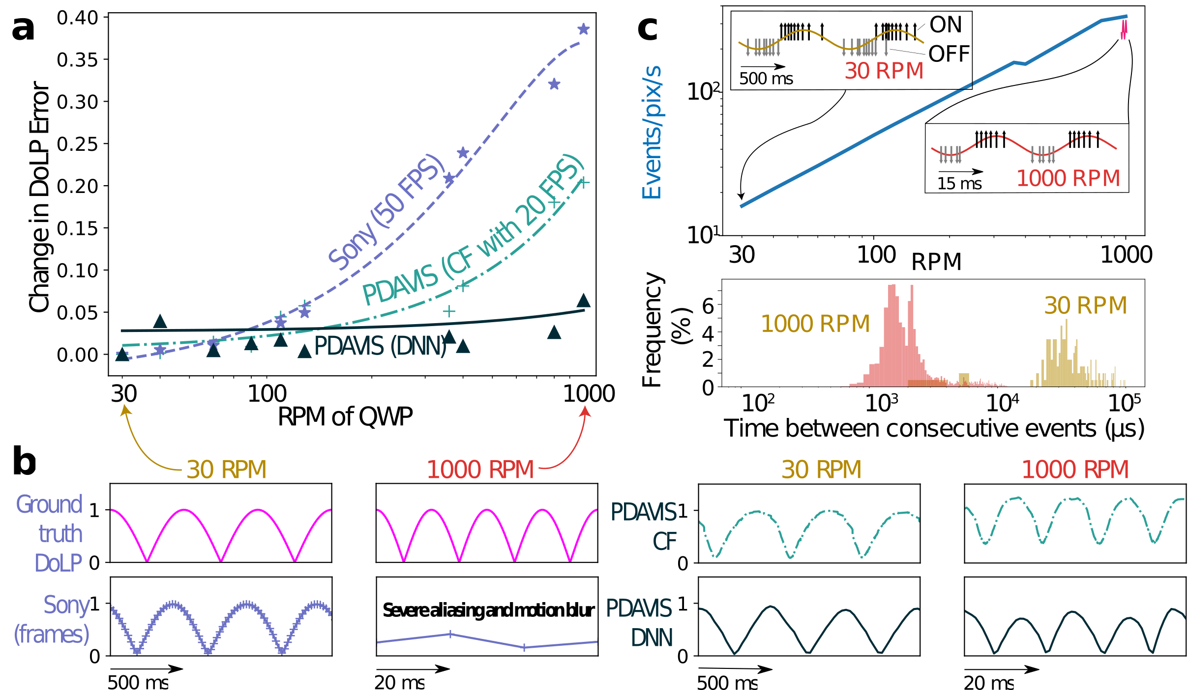
Figure 3: Comparison of frame-based and event-based reconstruction of DoLPDegree of Linear Polarization with various rotation speeds of a QWPQuarter Wave Plate. Each cycle of QWPQuarter Wave Plate rotation produces four cycles of DoLPDegree of Linear Polarization. a Growth of the mean absolute error of DoLPDegree of Linear Polarization reconstruction with RPM. The Sony has only synchronous intensity frames (see Supplementary Material 2.1). The CFComplementary Filter method fuses PDAVISPolarization Dynamic and Active pixel VIsion Sensor frames and events (see Supplementary Material 2.3). The DNNDeep Neural Network method uses only events (see Supplementary Material 2.4). b Reconstruction of the absolute DoLPDegree of Linear Polarization from a 100 pixel ROIRegion of Interest using various methods. The frame based Sony reconstruction is most accurate at low frequency but is severely aliased at 1000 RPM, which is not true for any of the PDAVISPolarization Dynamic and Active pixel VIsion Sensor methods using events. c Statistics of events. Upper plot is event rate versus QWPQuarter Wave Plate RPMRevolutions per Minute. Insets show actual ON and OFF events from a subpixel in response to the sinusoidal intensity variation. Lower plot shows histograms of the time between two consecutive events for the two rotational speeds of the QWPQuarter Wave Plate.

The third experiment (Fig. 4a, Supplementary Videos 3 and 4) compares the PDAVISPolarization Dynamic and Active pixel VIsion Sensor and Sony dynamic range. We imaged set of polarization filters offset by 30°rotating at 200 RPMRevolutions per Minute (5 rev/s) under high contrast 2000:1 lighting, such as commonly encountered in remote sensing of natural environments. The Sony camera exposure is set to 20 ms to capture the darker part of the scene without underexposing it, which overexposes and saturates the brighter part, preventing AoPAngle of Polarization measurement. The large motion blur is visible in the I0 image and incorrect AoPAngle of Polarization in the blurred regions. The PDAVISPolarization Dynamic and Active pixel VIsion Sensor can measure the AoPAngle of Polarization in both lighting conditions. Even though the PDAVISPolarization Dynamic and Active pixel VIsion Sensor frame is also motion blurred, all event-based methods produce sharp images.

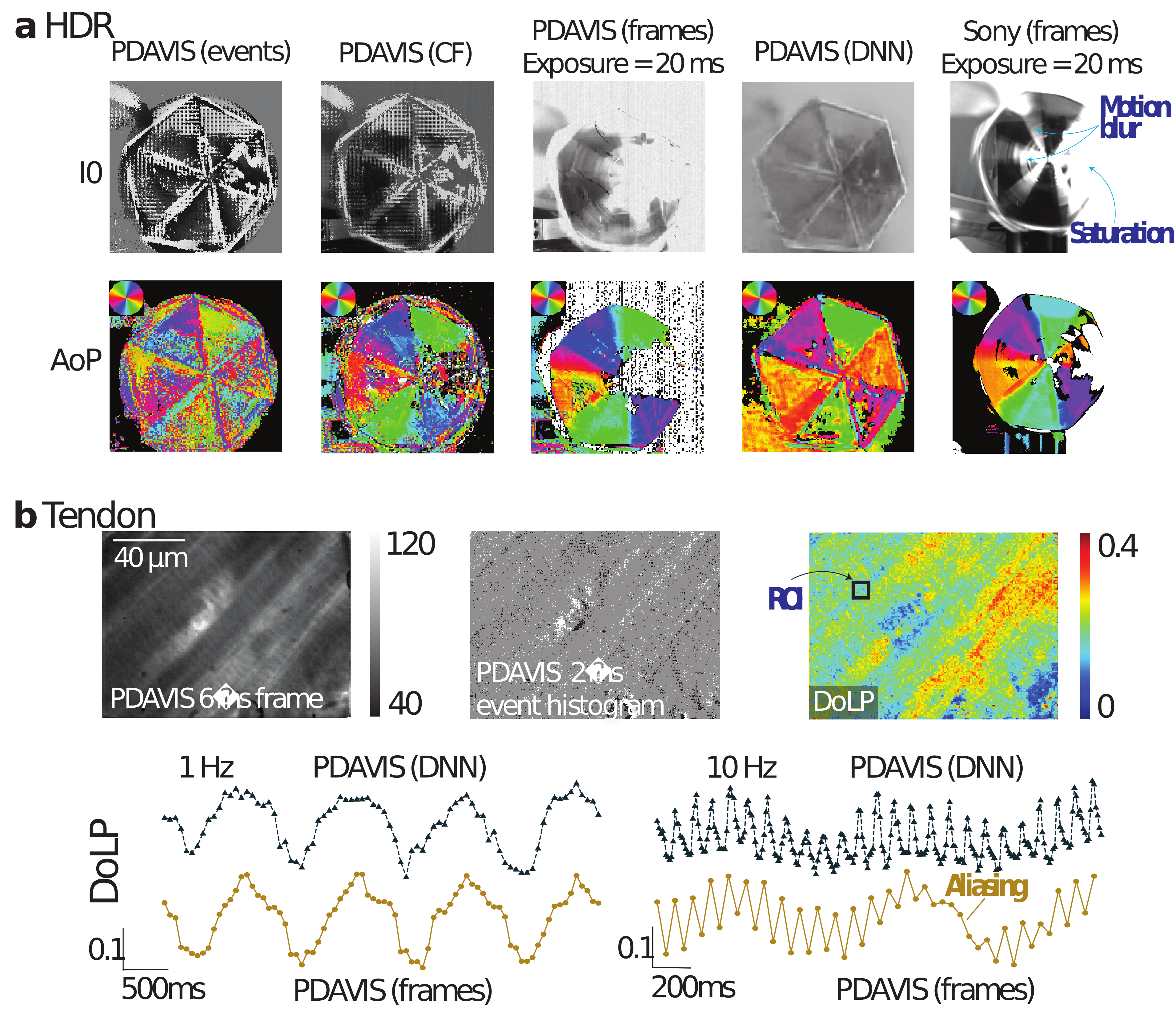
Figure 4: Applications of PDAVISPolarization Dynamic and Active pixel VIsion Sensor for remote sensing and scientific imaging. a Images of a rotating fan polarizer under HDRhigh dynamic range illumination captured by the PDAVISPolarization Dynamic and Active pixel VIsion Sensor and Sony’s camera using various reconstruction methods (see Supplementary Material 2). The fan is constructed from triangular linear polarizers arranged with 30° AoPAngle of Polarization spacing. The illumination ratio between bright and dark parts is 2000 and the rotation speed is 200 RPM. The I₀ images show reconstructed monochromatic intensity from pixels with 0 degree pixelated polarization filters of Fig. 1. The weakly-polarized regions in the AoPAngle of Polarization images are masked out using the measured DoLPDegree of Linear Polarization. b Imaging a tendon that is periodically stretched at 1 Hz and 10 Hz. The images (upper half) show a single frame (left), an event time window (center) and the corresponding DoLPDegree of Linear Polarization reconstruction result (right) using the DNNDeep Neural Network method (see Supplementary Material 3 and Supplementary Material 2). The event time window is rendered from a fixed time interval where ON (white) and OFF (black) events are accumulated to the starting gray image. The DNNDeep Neural Network input is 3D event tensors (the frames are not used) that have a duration of 50 ms or 10 ms, resulting in output at 20 or 100 FPSFrames Per Second for 1 Hz and 10 Hz respectively. The traces (lower half) compare the DNNDeep Neural Network and frame-based reconstructed DoLPDegree of Linear Polarization, averaged over the ROIRegion of Interest indicated in the DoLPDegree of Linear Polarization image (upper right). With 1 Hz stretching (left), both methods yield similar results. With 10 Hz stretching (right), the DNNDeep Neural Network reconstructs the DoLPDegree of Linear Polarization while the 20 FPSFrames Per Second frame-based reconstruction is severely aliased.

The fourth experiment (Fig. 4b, Supplementary Video 5) shows a potential medical imaging application of the PDAVISPolarization Dynamic and Active pixel VIsion Sensor (see Methods and Supplementary Material 3). We imaged the dynamics of a bovine tendon subjected to cyclical stress, such that its birefringent properties are time varying. As circularly polarized light transmits through the tendon, it becomes elliptically polarized and the DoLPDegree of Linear Polarization provides an indirect measurement of the birefringent properties, assuming minimal scattering. Using high optical magnification, we can observe strain patterns over time of the individual collagen fibers that comprise the tendon. Due to the high optical magnification and rapid movement of the collagen fibers, preventing aliasing would require a frame rate that is a large multiple of the cycle rate. By contrast, DNNDeep Neural Network reconstruction of the DoLPDegree of Linear Polarization (using only events) provides measurement of the dynamic properties of the individual collagen fibers at higher frequency than the maximum frame rate.

4 Discussion

Airborne, underwater, and space-based applications can require high temporal resolution and HDRhigh dynamic range, together with spectral and polarization sensitivity. All of these requirements increase the data rate, but the bioinspired sparse data streams and local gain control of event cameras enables near-sensor processing with low latency and a small computational footprint together with HDRhigh dynamic range. To compare PDAVISPolarization Dynamic and Active pixel VIsion Sensor with state-of-the-art polarization sensors, we developed novel event-driven reconstruction algorithms and compared their angle and degree of polarization reconstruction abilities to the frame-based camera reconstruction. The pure event-driven algorithm is the most economical, but it cannot reconstruct the degree of linear polarization, which requires an estimate of the absolute intensity which the event stream does not provide. The CFComplementary Filter helps to overcome this limitation by fusing the event stream with periodically captured frames while only slightly increasing the computational cost. The DNNDeep Neural Network provides the most accurate reconstruction, but requires a power hungry and expensive GPUGraphics Processing Unit for real time operation, which may not be affordable in a remote environment close to the sensor or with minimum latency. A limitation of the PDAVISPolarization Dynamic and Active pixel VIsion Sensor is with dense scenes, which can saturate the event output capacity, causing event loss. In these situations, a conventional frame-based polarization camera could be better suited. By adopting a bioinspired combination of sustained and transient pathway, the PDAVISPolarization Dynamic and Active pixel VIsion Sensor bridges a gap between the limited temporal and dynamic range of conventional frame-based polarization cameras and complex solid state imagers[23] or streak cameras[24] that can record short sequences at $>10^{7}$ FPSFrames Per Second. This gap is normally filled by high frame rate cameras that consume a lot of power and demand bright lighting for the short exposure times. The PDAVISPolarization Dynamic and Active pixel VIsion Sensor enables continuous AoPAngle of Polarization and DoLPDegree of Linear Polarization measurement with high contrast illumination at frequencies several times the Nyquist rate of frame-based image sensors. The PDAVISPolarization Dynamic and Active pixel VIsion Sensor event output triggers data acquisition and processing only when needed making it ideally matched with the increasing development of activation-sparsity aware neural accelerators[25, 26, 27].

5 Methods

The PDAVISPolarization Dynamic and Active pixel VIsion Sensor Polarization Filter Array (PFA) is fabricated on a quartz wafer using interference lithography and reactive ion etching. Reactive ion etching transfers the photoresist pattern to the silicon dioxide, which serves as a hard mask for etching the underlying aluminum. The filter array is then laser cut to match the total size of the pixel array. The individual polarization filters are comprised of aluminum nanowires with 70 nm width, 70 nm spacing, and 150 nm height, and have extinction ratio of  40 at 500 nm incident light (see Methods, Supplementary Material 1, and Supplementary Figs. S3 and  S4). The PFAPolarization Filter Array and pixel array are aligned using a 6-DOFDegree of Freedom positioning stage and are bonded using ultraviolet-curing optical adhesive. (see Supplementary Table 1).

A custom PCB hosts the PDAVISPolarization Dynamic and Active pixel VIsion Sensor chip and streams data (frames and events) to the host computer (see Supplementary Material 1.1 and Supplementary Fig. S1). To recover and reconstruct information about AoPAngle of Polarization and DoLPDegree of Linear Polarization we compared 4 different PDAVISPolarization Dynamic and Active pixel VIsion Sensor methods (for an overview see Supplementary Table 2, Supplementary Material 2). It also enabled a comparison with Sony’s camera (see Supplementary Table 1, Figs. S4,S5). We applied conventional frame-based reconstruction, purely event-driven reconstruction, event-frame sensor fusion, and a deep recurrent convolutional neural network (see Supplementary Material 2, Fig. S6). For Fig. 4b, we sectioned bovine tendons and mounted them on a custom-built stage to enable cyclical loading, and imaged them with a microscope objective (see Supplementary Material 3).

6 Data availability

The data that support the findings of this study are available within the article and its Supplementary Information. Raw data collected from the sensors are available upon request from V.G. or T.D.

7 Code availability

Software code and data used to generate polarization data are available online. The link will be made available once the paper is accepted for publication.

8 Funding

Fabrication of the polarization filters and travel was partially funded by the Swiss National Science Foundation Sinergia projects #CRSII5-18O316, #CRSII5-18O316 and ONR Global-X N62909-20-1-2078. This material is based upon research supported by, or in part by, the U. S. Office of Naval Research (N62909-20-1-2078, N00014-19-1-2400 and N00014-21-1-2177) and U.S. Air Force Office of Scientific Research (FA9550-18-1-0278).

9 Acknowledgments

The authors thank Greg Cohen, Tom Cronin, and Andrey Kaneev for comments; Cedric Scheerlinck for help with implementing the CFComplementary Filter; Steven Blair and Alex Pietros for help with aligning and bonding the polarization filter arrays to the DAVIS sensors; Steven Blair, Zuodong Liang, Colin Symons, and Zhongmin Zhu for help with measurements; Steven Blair and Zhongmin Zhu for help with data analysis; and Leanne Iannucci and Spencer Lake for assistance with the tendon experiments.

10 Author Contributions

T.D. and V.G. conceived the idea and supervised the project. G.H. and V.G. aligned and bonded the polarization filter arrays to the DAVIS sensors. DAVIS sensor was developed by T.D lab. Measurements were performed by D.J., Y.C., and J.H. Complementary filter was developed by T.D., G.H. and D.J. DNN data analysis was performed by J.H and Y.C. G.H., D.J., T.D., and M.B.M developed the event-based reconstruction algorithm. All authors contributed to the data analysis and writing of the paper.

Supplementary Materials

• Supplementary Material 1 provides details of the Polarization Dynamic and Active pixel VIsion Sensor (PDAVIS) pixel circuit, characterization setup, Polarization Filter Array (PFA) assembly, and specifications of the PDAVISPolarization Dynamic and Active pixel VIsion Sensor and Sony cameras.

• Supplementary Material 2 provides details of PDAVISPolarization Dynamic and Active pixel VIsion Sensor algorithms for reconstructing polarization.

• Supplementary Material 3 describes the setup of the bovine tendon experiment.

• Supplementary Video 1: The video shows both the frame and event based polarization reconstruction when a linear polarization filter is rotated in front of the PDAVIS camera. The top half of the video represents data acquired from the PDAVIS frames and the bottom half corresponds to event based reconstruction using complementary filter. The left half of the video depicts the intensity data from the four pixelated polarization filters. The right half of the video depicts the reconstructed angle of polarization. It can be observed that the frame based reconstruction (top right) updates Angle of Polarization (AoP) information at much slower speed compared to the event based reconstruction (bottom right). This video demonstrates the aliasing problems associated with frame based polarization imaging.

• Supplementary Video 2: The video shows both the frame and event based polarization reconstruction when a Quarter Wave Plate (QWP) filter is rotated in front of the PDAVISPolarization Dynamic and Active pixel VIsion Sensor camera. The top half of the video represents data acquired from the PDAVISPolarization Dynamic and Active pixel VIsion Sensor frames and the bottom half corresponds to event based reconstruction using the complementary filter. The left half of the video depicts the intensity data from the four pixelated polarization filters. The right half of the video depicts the reconstructed Degree of Linear Polarization (DoLP). It can be observed that the frame based (top right) updates DoLPDegree of Linear Polarization information at much slower speed compared to the event based reconstruction (bottom right). This video demonstrates the aliasing problems associated with frame based polarization imaging.

• Supplementary Video 3: The video shows a high dynamic range scene comprised of six linear polarization filters rotating at ~105 RPM. The frame based data from both Sony and PDAVIS cannot fatefully reconstruct the AoPAngle of Polarization across the entire scene due to the limited dynamic range. The event based reconstruction methods leverage the high dynamic range capabilities of the PDAVIS and reconstruct AoPAngle of Polarization information across the entire scene. Furthermore, slight motion blur can be observed in both intensity and AoPAngle of Polarization images in the Sony sensor.

• Supplementary Video 4: The video shows motion blur problems associated with frame based polarization sensor. The filter wheel is rotated at ~1000 RPM (16.7 rev/s), causing severe motion blur in the Sony polarization sensor. Due to the ”on-demand” imaging capability provided by events in the PDAVIS, motion blur in this experiment is non existent.

• Supplementary Video 5: Imaging single fibers of a bovine tendon under cyclical load of 1 Hz and 10 Hz. The frame based method can accurately monitor the changes of stress in single tendon fibers based on the AoPAngle of Polarization information. However, at 10 Hz cyclical load this information is severely aliased. Event based reconstruction provides updates only at the location of the fibers and provides accurate stress information at the 10 Hz cyclical load.

Supplementary Material 1 PDAVIS camera

Supplementary Material 1.1 PDAVIS chip

The DAVISDynamic and Active pixel VIsion Sensor chips used to build the PDAVISPolarization Dynamic and Active pixel VIsion Sensor cameras were fabricated by Towerjazz Semiconductors in their Fab 2 (Migdal HaEmek, Israel), a 180nm 6-metal CMOS Image Sensor (CIS) process with optimized buried photodiodes, antireflection coating, and customized microlenses for large pixels. The chips are packaged in a ceramic PGA package with a taped glass lid, which we remove for PFAPolarization Filter Array assembly (Supplementary Material 1.3).

Fig. S1 shows the PDAVISPolarization Dynamic and Active pixel VIsion Sensor pixel circuit. The design is based on the Dynamic Vision Sensor (DVS) [28] and the Dynamic and Active pixel VIsion Sensor (DAVIS) [29] with improvements described in [30].

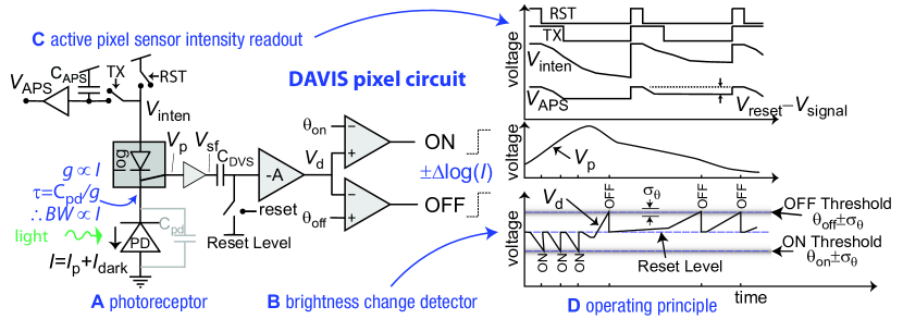
Figure S1: DAVISDynamic and Active pixel VIsion Sensor pixel circuit and operating principle. The sensor generates asynchronous brightness change ON and OFF DVSDynamic Vision Sensor events and APSActive Pixel Sensor intensity samples.

For the DVSDynamic Vision Sensor brightness change events, the logarithmic photoreceptor (A) drives a change detector (B) that generates the ON and OFF events (D). Pixel photoreceptors continuously transduce the photocurrent $I$ produced by the photodiode (PD) to a logarithmic voltage $V_{\text{p}}$, which results in over 120 dB dynamic range sensitivity. This logarithmic voltage (called brightness here) is buffered by a unity-gain source follower to the voltage $V_{\text{sf}}$, which is stored in a capacitor $C_{\text{DVS}}$ inside individual pixels, where it is continuously compared to the new input. If the change $V_{\text{d}}$ in log intensity exceeds a critical event threshold, an ON or OFF event is generated, representing an increase or decrease of brightness. The event thresholds $\theta_{\text{on}}$ and $\theta_{\text{off}}$ are nominally identical for the entire array. The time interval between individual events is inversely proportional to the derivative of the brightness. When an event is generated, the pixel’s location and the sign of the brightness change are immediately transmitted to an arbiter circuit surrounding the pixel array, then off-chip as a pixel address, and a timestamp is assigned to individual events. The arbiter circuit then resets the pixel’s change detector so that a new event can be generated by the pixel. Events can be read out from PDAVISPolarization Dynamic and Active pixel VIsion Sensor at up to rates of about 10 MHz. The quiescent (noise) event rate is a few kHz.

Non-idealities of the DVSDynamic Vision Sensor part of the pixel include 1) finite response time $\tau$ caused by the intensity-dependent RC time constant of the photoreceptor voltage $V_{\text{p}}$ as indicated in the photoreceptor circuit (A), 2) pixel-to-pixel mismatch $\sigma_{\theta}$ of the brightness change thresholds $\theta_{\text{on}}$ and $\theta_{\text{off}}$ (D), and 3) noise in the output [31, 32]. These non-idealities lead to background activity [31, 32] and Fixed Pattern Noise (FPN) [28] in the DVSDynamic Vision Sensor responses and finite DVSDynamic Vision Sensor motion blur [33] but in typical operating conditions the temporal jitter of event timing is less than 1 ms [33].

For the frames, the intensity samples are captured by the APSActive Pixel Sensor readout circuit (C). The absolute intensity is measured by the photocurrent passing non-destructively through the photoreceptor circuit, where it is integrated onto a capacitor $C_{\text{APS}}$, whose voltage $V_{\text{inten}}$ is read out via a source follower transistor as $V_{\text{APS}}$ similar to conventional CMOS image sensors. At the start of each frame, the global signal RST pulls all pixel $V_{\text{inten}}$ high. The reset level of each pixel is read out from $V_{\text{APS}}$ through column-parallel Analog to Digital Converters (ADC) (not shown). At the end of integration, TX freezes the sampled $V_{\text{inten}}$ signal on $C_{\text{APS}}$ and the signal values are read out. Each final intensity sample is the difference between the reset level and signal level. The on-chip column-parallel 10-bit ADCsAnalog to Digital Converter convert the samples of reset and signal and subtraction is computed in software on the host computer. The frame-based output can generate videos with a desired exposure time – where all pixels have the same integration (or exposure) time – down to about 10 us and up to the frame interval. Readout speed limits the maximum frame rate to about 50 Hz.

Events and frames are transmitted from the DAVISDynamic and Active pixel VIsion Sensor chip to a host computer over Universal Serial Bus (USB) via a programmable logic chip[34]. Each frame pixel sample is 10 bits occupying a (non optimized) 2 bytes. Each event is transmitted using a 16-bit microsecond timestamp and from 2 to 4 bytes address depending on data rate (the DAVISDynamic and Active pixel VIsion Sensor uses Boahen’s word-serial Address Event Protocol (AER) interface [35]); at high data rate, most events use only 2 bytes for their column address, since events from the same row within a short time interval share the same timestamp.

Supplementary Material 1.2 PDAVIS Characterization Setup

Fig. S2-a depicts the experimental setup used to evaluate the optoelectronic properties for both PDAVIS and Sony polarization cameras when rotating a linear polarization filter at different speeds. A narrow band LED light source (LZ4-00G108, Osram) centered at 520 nm is coupled to a 6” integrating sphere (819D-SF-5.3, Newport). The light exiting the integrating sphere is uniform and depolarized due to the multiple scattering events inside the integrating sphere. A custom-built rotational stage is placed in front of the output port of the integrating sphere. The rotational stage is controlled via a 10:1 stepper gear and a DC motor with a feedback controller. The rotational speed of the stage is controlled from a computer and can rotate up to 3,000 RPM. Due to the feedback controller, the rotational speed is within 10 RPM of the desired value.

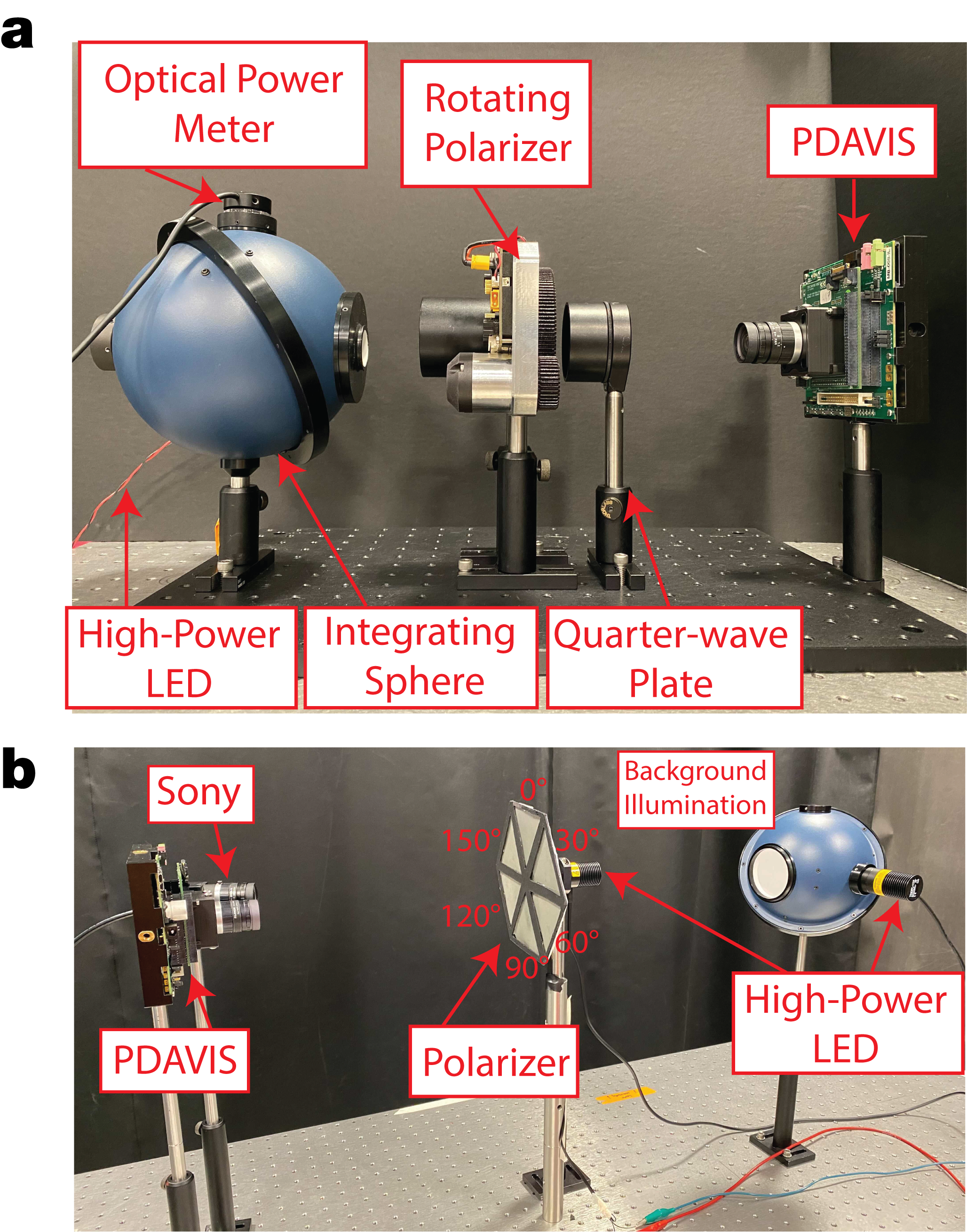
Figure S2: a Photo of the characterization bench, built around the integrating sphere to generate an unpolarized light, filtered through either a linear polarizer or a combination of linear polarizer and a QWPQuarter Wave Plate to generate different AoPAngle of Polarization and DoLPDegree of Linear Polarization profiles while an optical power meter measures the irradiance level. Data is collected with either Sony or PDAVISPolarization Dynamic and Active pixel VIsion Sensor sensor. b Experimental setup used for collecting data under high dynamic range and rotating ensemble of six linear polarization filters offset by 30 °.

For the first set of experiments, a linear polarization filter (20LP-VIS-B, Newport) is placed in the rotational stage opening. The light emerging from the rotating filter is imaged with either PDAVIS or Sony’s polarization camera. When a linear polarization filter is rotated in front of the camera, the angle of polarization is varied between 0 and 180 degrees. One full rotation of the linear polarization filter will generate two full cycles of the AoPAngle of Polarization. The rotational speed of the filter was varied between 60 RPM and 1,000 RPM.

For the second set of experiments, a zero-order QWPQuarter Wave Plate filter (20RP34-532, Newport) is placed after the rotational stage housing the linear polarization filter and before the imaging sensor. The orientation of the QWPQuarter Wave Plate is fixed while the linear polarization filter is rotated at constant speed. When the linear polarization filter is rotated in front of the camera, both the angle and degree of linear polarization are varied. One full rotation of the linear polarization filter will generate four full cycles of the AoPAngle of Polarization and DoLPDegree of Linear Polarization.

Fig. S2-b depicts the experimental setup used to evaluate the high dynamic range and motion blur for both PDAVIS and Sony polarization cameras when rotating an ensemble of six linear polarization filter offset by 30 ° at different speeds. A narrow band LED light source (LZ4-00G108, Osram) centered at 520 nm is coupled to a 6” integrating sphere (819D-SF-5.3, Newport). The output light from the integrating sphere is incident on the ensemble of linear polarization filters. A high intensity LED is placed behind the filter wheel to provide additional light intensity. The filter wheel is mounted on a motor such that the filters are rotated at different speeds. Images are collected with both Sony and PDAVIS sensors.

Supplementary Material 1.3 Fabrication of PDAVIS

The pixelated PFAsPolarization Filter Array were fabricated on a quartz substrate by Moxtek Inc. The PFAPolarization Filter Array contains four sets of pixels with linear polarization filters offset by 45 degrees. The pixel pitch of the filter array is 18.5 microns and matches the pitch of the pixels in the DAVIS vision sensor. Pixels are isolated by a 2 um-wide metal shield.

The steps (illustrated in Fig. S3) to integrate the PFAPolarization Filter Array with the packaged DAVISDynamic and Active pixel VIsion Sensor chip (Supplementary Material 1.1) are based on a method initially presented by Blair et al.  [36] and expanded upon below:

1. The quartz glass with the PFAPolarization Filter Array is glued to a secondary cover glass using a UV activated and optically transparent epoxy (OP-29, Dymax). The cover glass has the same dimensions as the ceramic package of the DAVISDynamic and Active pixel VIsion Sensor (Fig. S3a).

2. The cover glass is mounted on a 3” by 3” glass plate using thermally activated bonding wax (part number) (Fig. S3b).

3. The glass plate is fixated on a custom-built flat stage and held via vacuum on the stage. The entire stage is fixed using 1” posts on a vibration damped optical table (Fig. S3c).

4. The DAVIS vision sensor is mounted on a 6-Degree of Freedom (DOF) alignment stage and placed under the cover glass stage (H-811 Hexapod, PI-USA Instruments). The alignment stage is initialized to the lowest position with about 2 cm space between the filter array and the sensor plane (Fig. S3d).

5. An integrating sphere (819D-SF-4, Newport) coupled with a high power red led (M660D2, Thorlabs) is placed 2 feet away from the DAVIS sensor. An adjustable iris (SM2D25, Thorlabs) followed by a linear polarization filter (WP25L-VIS, Thorlabs) mounted on a computer-controlled rotational stage (HDR50, Thorlabs) is placed at the output of the integrating sphere. The center of the output port of the integrating sphere is aligned with the center of the vision sensor. Due to the large distance between the integrating sphere and the vision sensor and the small aperture of the iris, the incident light is collimated and linearly polarized (Fig. S3e).

6. Live images are streamed from the DAVIS sensor and custom software is used to provide statistics about the vision sensor, such as the mean and standard deviation of individual pixels in the image array as well as extinction ratios between orthogonal pixels.

7. As the vision sensor is brought closer to the filter array, first the pitch and yaw are adjusted, followed by x- and y- adjustments. For each positional adjustment, the linear polarization filter in front of the vision sensor is rotated, which enables evaluation of the extinction ratios (Fig. S3f).

8. The vision sensor is considered in contact with the pixel array when the extinction ratios remain constant. At this point, the aperture is increased to generate less collimated light. If the extinction ratios remain the same, then the filter is in contact with the sensor.

9. The DAVIS sensor is then lowered away from the filter array. A UV activated epoxy is added to the ceramic package of the DAVIS sensor and the sensor is brought slowly into contact with the filter array. Because the camera was only translated in the z direction during this step, it remains in good alignment with the filter array. Small positional adjustments can be made if necessary. Since the light source used for imaging does not have any UV component, the epoxy does not cure during the alignment process.

10. A UV light source is used to activate the epoxy and permanently attach the filters to the ceramic package. The UV light will cure 99% of the epoxy within the first 15 to 30 seconds. However, 100% of the epoxy is cured after 24 hours of UV exposure. The filters and vision sensors remain in the alignment stage for 24 hours under UV light to completely cure the epoxy.

11. Next, the vacuum is turned off so that the glass plate can be removed from the alignment stage without damaging the vision sensor and glued filters. The camera is lowered and removed from the alignment instrument (Fig. S3g).

12. The glass plate is removed by applying heat from a hot plate at 80 C. Any residual bonding wax on top of the vision sensor is cleaned with acetone-soaked cotton swabs (Fig. S3h).

The completed PDAVISPolarization Dynamic and Active pixel VIsion Sensor is shown in Fig. S3i. The pixelated polarization filters are aligned and in contact with the DAVIS pixel array. The filters are attached to a secondary cover glass slide and glued to the ceramic package of the DAVIS chip.

Fig. S3j shows an SEM image of the four different orientations of the nanowires within individual pixelated polarization filters.

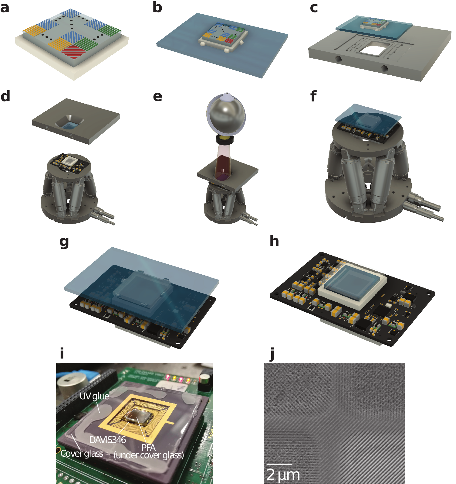
Figure S3: Fabrication steps of the PDAVISPolarization Dynamic and Active pixel VIsion Sensor PFAPolarization Filter Array. a Quartz glass with PFAPolarization Filter Array is glued to a cover glass. b Cover glass is mounted on a glass plate. c Glass plate is vacuum-fixed to flat stage, d and e The polarization filter stack is positioned during live operation of the PDAVISPolarization Dynamic and Active pixel VIsion Sensor to the die. f Polarization filter stack is aligned and attached to the vision sensor. g Complete image sensor removed from alignment stage. h Glass plate is removed from the polarization sensor i Photo of the assembled PDAVISPolarization Dynamic and Active pixel VIsion Sensor. The PFAPolarization Filter Array is attached to the bottom of the coverglass. j SEM image of PFAPolarization Filter Array.

Supplementary Material 1.4 Extinction ratio measurements

The following setup is constructed to measure the Extinction Ratio (ER) of PDAVIS as a function of wavelength. We start by using a 400 W halogen light bulb (7787XHP, Philips) housed in a custom box and powered by a high power voltage supply (N5770A, Agilent). The light from the halogen bulb is directed into a monochromator (Acton SP2150, Princeton Instruments), where the desired wavelength is selected using a grating and a computer-controlled slit at the output port. Since the output light beam is typically partially polarized, an integrating sphere (819D-SF-4, Newport) is placed at the output port of the monochromator to depolarize the monochromatic light beam. A pinhole (SM2D25, Thorlabs) followed by an aspherical lens (ACL5040U, Thorlabs) are used to collimate the light beam emerging from the integrating sphere. Lastly, a linear polarization filter (WP25L-VIS, Thorlabs) mounted on a computer-controlled rotational stage (HDR50, Thorlabs) is used to produce collimated and linearly polarised monochromatic light which is imaged by either the PDAVIS sensor or a spectrometer. The spectrometer is used to measure the exact wavelength of the incident light on the vision sensor. An optical power meter is placed at the same location where the image sensor is located and used to measure the photon flux of the incident light at the desired wavelength.

With the setup described above, we first recorded 100 frames with all light blocked from the sensor. These 100 frames, subsequently called dark frames, are temporally averaged to find the digital number offset for each pixel caused by imperfections of the pixel’s circuitry. Next, the monochromator is turned on and set to output monochromatic light at a particular wavelength. The linear polarization filter is rotated 180° in increments of 5°. A total of 100 frames are recorded for each angle and are spatiotemporally averaged over a 42x28 macropixel Region of Interest (ROI). The 180° sweep over a single wavelength gives us one period of Malus’s Law (Supplementary Material 2.1, Eq. (S8)). A non-linear regression then fits the cosine squared signal reconstructed from the linear polarizer sweep. After subtracting the dark frame to remove noise offsets, the ERExtinction Ratio (the reciprocal of the ratio of cross-polarized light that passes the linear polarizer is computed by taking the ratio of the largest and smallest digital number from the cosine squared function. This process is repeated over the range of wavelengths from 500nm to 700nm in steps of 20nm to give us the extinction ratio for each filter in the macropixel. The results are shown in Figure  S4.

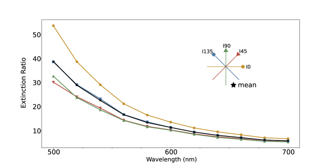
Figure S4: Measured extinction ratios vs. wavelength for the PDAVIS sensor.

Supplementary Material 1.5 Dynamic range for polarization sensitivity

To measure the Dynamic Range (DR) over which the PDAVIS or Sony sensors are sensitive to linearly polarized light, we constructed the following optical setup. A custom-built high power, water-cooled white LED light source (CXB3590, Digikey) is coupled to a 4” integrating sphere (819D-SF-4, Newport). The LED power is adjusted by a computer-controlled power supply (N5770A, Agilent). The light exiting the integrating sphere is uniform and depolarized due to the multiple scattering events inside the integrating sphere. A linear polarization filter (WP25L-VIS, Thorlabs) mounted on a computer-controlled rotational stage (HDR50, Thorlabs) is placed at the output of the integrating sphere. The linear polarization filter is rotated at 60 RPM. Hence, time-varying linearly polarized light at different intensity levels is used to illuminate either the PDAVIS or Sony polarization camera.

The Sony camera exposure time is set to 20 ms for this set of optical experiments. This mimics a situation where in order for the dark parts of the imaged scene to have a nonzero digital value, the minimum exposure time should be at least 20 ms. The PDAVISPolarization Dynamic and Active pixel VIsion Sensor pixels has a local gain/exposure control by virtue of the logarithmic photoreceptors, and thus there is no need to set any exposure time because the frames are not used for the Deep Neural Network (DNN) reconstruction method. For each illumination levels, both Sony and PDAVISPolarization Dynamic and Active pixel VIsion Sensor capture polarization information from a ROIRegion of Interest of 20x20 macropixel corresponding to the rotating linear polarization filter. For the Sony camera, AoPAngle of Polarization is computed from the raw intensity information from the four super pixels and spatially averaged across the ROIRegion of Interest. For the PDAVISPolarization Dynamic and Active pixel VIsion Sensor, we first reconstruct the intensity for the four individual channels of polarized pixels using the DNNDeep Neural Network method (which uses only the brightness change events) (see Supplementary Material 2.4), and then computed the spatially averaged AoPAngle of Polarization within the ROIRegion of Interest. Since the linear polarization filter was rotating at a steady speed, the AoPAngle of Polarization is a repeated sawtooth linear response, sweeping between 0° and 180°. However, once the illumination level exceeds the DRDynamic Range of the camera, the saturated pixels will result in incorrect AoPAngle of Polarization computation and thus the range of the reconstructed AoPAngle of Polarization is smaller than the expected 180°.

The Fig. S5 results show the range of AoPAngle of Polarization reconstruction angles for the sawtooth variation, over illumination level ranging from 40 nW/cm² to 42 mW/cm². It demonstrates that the Sony camera can reconstruct the AoPAngle of Polarization between 40 nW/cm² and 300 $\mu$W/cm² optical flux, corresponding to a dynamic range of 77.5 dB (7300X). Beyond 300 $\mu$W/cm² optical flux, all Sony pixels are saturated and the polarization sensitivity vanishes. By contrast, the PDAVISPolarization Dynamic and Active pixel VIsion Sensor is able to reconstruct nearly the full 180° sawtooth over 120 dB illumination levels, from 40 nW/cm² to 42 mW/cm² optical power.

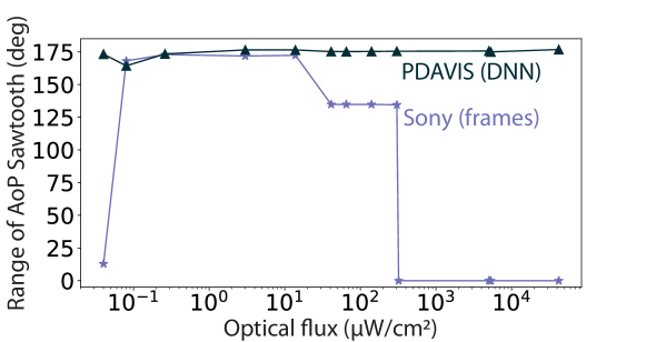
Figure S5: Measured dynamic range for polarization sensitivity for PDAVIS and Sony’s polarization sensors . The AoPAngle of Polarization axis is the amplitude of the reconstructed sawtooth as the linear polarization filter is rotated 180 degrees.

Supplementary Material 1.6 PDAVIS and Sony camera specifications

Table 1 compares the design and measured specifications of the PDAVISPolarization Dynamic and Active pixel VIsion Sensor with a state-of-the-art Commodity Off-The-Shelf (COTS) frame-based polarization camera (FLIR BFS-U3-51S5), which uses the Sony IMX250 camera chip. Details of our measurements of dynamic range and extinction ratio of PDAVISPolarization Dynamic and Active pixel VIsion Sensor precede this section.

The Sony polarization sensor has higher resolution, smaller pixel size, and higher extinction ratio. Our bioinspired sensor is fabricated at several different locations: the event-based sensor is fabricated in a 180nm CIS process provided by TowerJazz Semiconductors; pixelated polarization filters are fabricated in Moxtek cleanroom facilities; the filters and image sensor are integrated at University of Illinois. Due to the complex fabrication steps, the image sensor pixel pitch is larger and the extinction ratios are lower than Sony’s sensor. The PDAVISPolarization Dynamic and Active pixel VIsion Sensor offers much higher temporal resolution ($\approx$100 us versus 12 ms) and its DVS output has superior DRDynamic Range compared to Sony polarization camera (120dB vs 72dB).

[!h] PDAVISPolarization Dynamic and Active pixel VIsion Sensor (this work) COTSCommodity Off-The-Shelf Sony IMX-250 CISCMOS Image Sensor Process 180nm 90/40nm stacked Pixel size 18.5$\mu$m 3.45$\mu$m Array size 346x260 2448x2048 Output APS+DVS+IMU APS Power consumption (camera) est. 3 W 3 W ERExtinction Ratio (the reciprocal of the ratio of cross-polarized light that passes the linear polarizer at 500nm 40 350 Max APS frame rate 53 Hz^a 75 Hz APS DR 52dB [29] 72 dB Max DVS event rate 10 MHz - DVS DR 120dB [29] - DVS Min latency 3us@1klux [29] - Min DVS threshold^b $\pm$14% - DVS threshold mismatch^c 3.5% [29] -

Table 1: Specification and comparison

• with exposure 80 us.

• At room temperature, with mean background leak activity rate of 0.7 Hz with background intensity from APS exposure of 26 DN/ms.

• Pixel to pixel 1-$\sigma$ mismatch of the threshold in temporal contrast.

Supplementary Material 2 Reconstructing polarization information from PDAVIS output

Supplementary Material 2.1 provides the definition of the Stokes parameters, AoPAngle of Polarization, and DoLPDegree of Linear Polarization. Supplementary Material 2.2 shows that using only the brightness changes (log intensity changes) signaled by the DVSDynamic Vision Sensor events from PDAVISPolarization Dynamic and Active pixel VIsion Sensor allows us to retrieve (at least) the change in AoPAngle of Polarization, because it depends on the ratio of differences of polarizer responses. However, for the DoLPDegree of Linear Polarization the absolute intensity does not cancel, and so it cannot be recovered solely from the brightness change events. The DAVIS APSActive Pixel Sensor frames, however, provide periodic absolute intensity samples. These samples have the limited DRDynamic Range and sample rate of frames, but by combining them with the DVSDynamic Vision Sensor events, we can reconstruct the absolute intensity with larger DRDynamic Range and higher sample rate, and thus polarization at high effective sample rates. We demonstrate two very different approaches for such absolute intensity reconstruction. The Complementary Filter (CF) (Supplementary Material 2.3) is based on a hand-crafted sensory fusion algorithm CFComplementary Filter, which fuses frames and events. The DNNDeep Neural Network method (Supplementary Material 2.4) is based on DNNsDeep Neural Network and infers intensity frames from brightness change events, based on its training data. Table 2 compares the methods.

For Figs. 2-3, the plotted AoPAngle of Polarization and DoLPDegree of Linear Polarization values are obtained by averaging over a $12\times 12$ pixel ROIRegion of Interest centered on the rotating polarizer.

Table 2: Comparison of approaches to reconstruct polarization information from the PDAVIS.

	DVSDynamic Vision Sensor	APSActive Pixel Sensor	AoPAngle of Polarization	DoLPDegree of Linear Polarization	Sampling rate [Hz]	Latency	Op/pixel
Events	✓	-	✓	-	10k	1 Event	12
Frames	-	✓	✓	✓	25	1 Frame	8
DNNDeep Neural Network	✓	-	✓	✓	10k	2k Events	41k
CFComplementary Filter	✓	✓	✓	✓	10k	1 Event or 1 Frame	14

Supplementary Material 2.1 Conventional Polarization Imaging

Polarization is commonly described using the Stokes parameters: $(S_{0},S_{1},S_{2})$ defined [37]:

$$S_{0}(t)=I_{0}(t)+I_{90}(t)$$ (S1)

$$S_{1}(t)=I_{0}(t)-I_{90}(t)$$ (S2)

$$S_{2}(t)=I_{45}(t)-I_{135}(t)$$ (S3)

where $I_{i}$ stands for the light intensity transmitted by the linear polarizer filter with angle $i$. A fourth Stokes parameter ($S3$) describes the circular polarization properties of the light field, which is not detected by the PDAVISPolarization Dynamic and Active pixel VIsion Sensor or Sony cameras. The DoLPDegree of Linear Polarization and the AoPAngle of Polarization can then be estimated from the Stokes parameters:

$$\text{DoLP}(t)=\frac{\sqrt{S_{1}(t)^{2}+S_{2}(t)^{2}}}{S_{0}(t)}$$ (S4)

$$\text{AoP}(t)=\frac{1}{2}\arctan\left(\frac{S_{2}(t)}{S_{1}(t)}\right)$$ (S5)

Equivalently, the incident light can be separated into unpolarized and linearly polarized beams, whose fluxes are $I_{\text{np}}$ and $I_{\text{p}}$, respectively. We also let the AoPAngle of Polarization be denoted by $\theta(t)$ and the total flux received by the photodiode by $I_{\text{t}}=I_{\text{np}}+I_{\text{p}}$. Thus, the DoLPDegree of Linear Polarization and the AoPAngle of Polarization can be defined by:

$$\text{DoLP}(t)\equiv\frac{I_{\text{p}}(t)}{I_{\text{t}}(t)}$$ (S6)

$$\text{AoP}(t)\equiv\theta(t)$$ (S7)

Since the intensity is proportional to the square of the electric field strength, the intensity of light passing through each polarizer is given by (S8) [37]:

$$I_{i}(t)=I_{t}(t)\text{DoLP}(t)\cos[\theta(t)-i]^{2}+\frac{I_{t}(t)}{2}(1-\text{DoLP}(t)).$$ (S8)

The second term of (S8) has the factor $\frac{1}{2}$ since half of unpolarized light passes through a filter.

Supplementary Material 2.2 Reconstructing AoP from PDAVIS events only

We can reconstruct the change in absolute log intensity $dL$ from an arbitrary starting point by simply integrating the events over time, as first studied experimentally by [38]. Pixel nonidealities cause this estimate to drift. The events method[39] regards the events as providing high frequency information about the log intensity change. Above a corner frequency ${f_{\text{3dB}}}=2\pi\omega=1/(2\pi\tau)$, the events directly update the filtered log intensity estimate, which decays to zero with time constant $\tau$ between events. Since the AoPAngle of Polarization depends only on ratios of differences of $I_{i}$ values, the absolute intensity factors out, so we can compute AoPAngle of Polarization from the reconstructed $I_{i}$ values.

For every incoming event, the events method asynchronously updates the related reconstructed log intensity change $dL=d\log(F)$ as the asynchronous first-order Infinite Impulse Response (IIR) filter (S9):

$$\begin{split}\alpha&\leftarrow e^{-\Delta t/\tau}\\ dL&\leftarrow\alpha dL+p\end{split}$$ (S9)

where $\Delta t$ is the time elapsed since last event from the subpixel, $\tau$ is the filter time constant, and $p=[+\theta_{\text{on}},-\theta_{\text{off}}]$ is the signed event threshold, which we estimate from the known bias currents using the formulas from [31] and then fine tune to match the low frequency frame-based data.

From the $dL$ values, we can compute AoPAngle of Polarization by exponentiation of $dL$ to obtain the subpixel $I_{i}$ value, and use the resulting $I_{i}$ values in (S5). In practice, we use the $dL$ values directly, since generally $|dL|<1$ and thus $\exp(dL)\approx 1+dL$. The 1 would be the same for all terms in (S5) and would thus cancel, leaving the $dL$ value.

The $dL$ in (S9) is the highpass-filtered log intensity, corresponding to the Laplace domain transfer function (S10):

$$H_{\text{dL}}(s)\equiv\frac{dL(s)}{\sum{p}(s)}=\frac{\tau s}{1+\tau s}$$ (S10)

where $s$ is the complex frequency, and $\sum{p}$ is the staircase sum of Dirac delta brightness changes since filter startup.

There are two exactly equivalent descriptions of this filter: $dL$ is a highpass-filtered log intensity, and it is also a lowpass-filtered derivative of log intensity. Thus, for frequencies well below the ${f_{\text{3dB}}}$ corner frequency $dL\approx\tau dL/dt$, $dL$ can be considered as a lowpass filtered derivative of $L$, which filters out derivatives above ${f_{\text{3dB}}}$. For frequencies well above ${f_{\text{3dB}}}$, $dL$ is equal to $L$ minus its DC value averaged over the exponential time window $\tau$. If we can assume that this offset is equivalent for each subpixel, then it cancels out in $S_{1}$ and $S_{2}$, which are used to compute the AoPAngle of Polarization.

For the events results in Figs. 1 and 2 we used ${f_{\text{3dB}}}=0.5\text{ Hz}$.

Effect of high pass filter on AoPAngle of Polarization: For input frequencies well above ${f_{\text{3dB}}}$, using the $dL$ values in (S5) results in the AoPAngle of Polarization if we make the reasonable assumption that all $I_{x}$ have the same mean value. For frequencies below ${f_{\text{3dB}}}$, where $dL\approx\tau dL/dt$, the following computation shows that using $dL$ in the AoPAngle of Polarization equation (S5) results in the AoPAngle of Polarization, but with a phase shift of $\pi/4$. First, we use (S8) to compute the derivative of $I_{i}$, where $i$ is one of the polarizer angles:

$$\frac{\partial I_{i}(t)}{\partial t}=-2I_{t}\text{DoLP}(t)\frac{\partial\theta(t)}{\partial t}\sin\left[\theta(t)-i\right]\cos\left[\theta(t)-i\right]$$ (S11)

Since we only care about measuring a varying AoPAngle of Polarization, we have assumed that DoLPDegree of Linear Polarization and $I_{t}$ are constant. Now we can plug (S11) into (S5):

$$\begin{split}\frac{1}{2}\arctan\left(\frac{\partial S_{2}/\partial t}{\partial S_{1}/\partial t}\right)&=\\ =&\frac{1}{2}\arctan\left(\frac{\partial I_{45}/\partial t-\partial I_{135}/\partial t}{\partial I_{0}/\partial t-\partial I_{90}/\partial t}\right)\\ =&\frac{1}{2}\arctan\left(\frac{2\sin(\theta-\frac{\pi}{4})\cos(\theta-\frac{\pi}{4})}{2\sin(\theta)\cos(\theta)}\right)\\ =&\frac{1}{2}\arctan\left(\frac{1}{-\tan(2\theta)}\right)\\ =&\theta(t)\bmod\pi+\frac{\pi}{4}\\ =&\text{AoP}(t)\bmod\pi+\frac{\pi}{4}\end{split}$$ (S12)

According to (S12), using the temporal derivatives of intensities in (S5) results in the AoPAngle of Polarization with a (constant $\pi/4$) offset.

In practice, we used signal periodicity to estimate the AoPAngle of Polarization phase in Fig. 2. Most of our experiments used a stimulus frequency above ${f_{\text{3dB}}}$, so the output of the AoPAngle of Polarization from the events method corresponds to the actual AoPAngle of Polarization without this offset. For example, Fig. 2c shows the reconstructed AoPAngle of Polarization sawtooth at 30 RPM, corresponding to an AoPAngle of Polarization frequency of 1Hz, which is double the ${f_{\text{3dB}}}=0.5\text{ Hz}$ corner frequency.

To lower the effect of mismatch and temporal noise, an event generated by the macropixel $(x,y)$ contributes to update the macropixels within a one pixel radius.

The AoPAngle of Polarization values are updated as soon as each event is received, creating polarization events as illustrated in Fig. 1c. These asynchronous updates could drive a quick event-driven processing pipeline that exploits the precise timing of events.

Source code for this algorithm is available .

Supplementary Material 2.3 Complementary Filter: Reconstructing AoP and DoLP by fusing frames and events

The CFComplementary Filter of Scheerlinck[39] is complementary because it considers APSActive Pixel Sensor frames as providing reliable low frequency intensity (albeit with limited DRDynamic Range), while the DVSDynamic Vision Sensor events provide reliable high frequency information about brightness (changes). The CFComplementary Filter method fuses the high pass filtered log intensity of the events method with low pass filtered frames. At the CFComplementary Filter crossover frequency $\omega=1/\tau=2\pi{f_{\text{3dB}}}$, the frame and event estimates of log intensity are weighted equally. For lower frequencies, the frame intensities are weighted more, and for higher frequencies, the event-based estimations are weighted more.

The CFComplementary Filter also has a computational cost of about 10 operations per DVSDynamic Vision Sensor event or APSActive Pixel Sensor sample, making it attractive for real-time applications.

At each subpixel, the CFComplementary Filter updates its log intensity reconstruction $L$ each time the pixel measures either intensity or generates a DVSDynamic Vision Sensor event. The CFComplementary Filter outputs the log intensity $L$ from the most recent log intensity sample or DVSDynamic Vision Sensor event. For each pixel’s APSActive Pixel Sensor intensity sample or DVSDynamic Vision Sensor event, the asynchronous first-order IIRInfinite Impulse Response filter CFComplementary Filter update is

$$\begin{split}\alpha&\leftarrow e^{-\Delta t/\tau}\\ L&\leftarrow\underbrace{\alpha L+p}_{\text{DVS}}+\underbrace{(1-\alpha)L_{\text{aps}}}_{\text{APS}}\end{split}$$ (S13)

where $\Delta t$ is the time since last update, $\tau=1/(2\pi{f_{\text{3dB}}})$ is the filter time constant, $p=[+\theta_{\text{on}},-\theta_{\text{off}}]$ is the event’s log intensity change, and $L_{\text{aps}}$ is the log intensity sample. (If the update is for an event, $L_{\text{aps}}=0$, or if the update is for a frame, $p=0$.) Since $\Delta t\ll\tau$ (the update rate is much higher than the time constant), $\alpha\approx 1-\Delta t/\tau\sim 1$. Removing the APSActive Pixel Sensor input from Eq. S13 gives the events method presented in the previous section (Eq. S9).

In the Laplace domain, the CFComplementary Filter filter has form (S14):

$$L(s)=\frac{\tau s}{1+\tau s}\sum{p(s)}+\frac{1}{1+\tau s}L_{\text{APS}}(s).$$ (S14)

Fig. S6 illustrates the equivalent continuous time CR highpass plus RC lowpass circuit for the CFComplementary Filter, along with the weighting of frames and events in the resulting CFComplementary Filter transfer function.

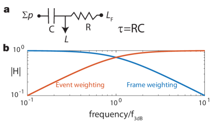
Figure S6: a Equivalent continuous-time circuit of CFComplementary Filter. b Magnitude transfer function of the CFComplementary Filter method.

For our experiments, we used CFComplementary Filter ${f_{\text{3dB}}}=1.6\text{ Hz}$. The AoPAngle of Polarization and DoLPDegree of Linear Polarization are periodically computed using the subpixel $L$ values. The user can decide this update rate; by default, the computation occurs at the end of each packet of PDAVISPolarization Dynamic and Active pixel VIsion Sensor data.

Adaptive gain tuning: The CFComplementary Filter method includes a downweighting of the APSActive Pixel Sensor samples when $L_{\text{aps}}$ approach their limits, are under or overexposed [39, Sec. 4.1]. We used this feature to improve the DRDynamic Range of the reconstruction. We set adaptive gain tuning $\lambda=0.1$ and used the limits $L_{1},L_{2}=\log(10,200)$.

Filter startup: To avoid the CFComplementary Filter filter startup transient, we initialize the filter output state to the first $L_{\text{APS}}$ frame as soon as it is available.

Source code for the original CFComplementary Filter implementation, our implementation of CFComplementary Filter, and for computing PDAVISPolarization Dynamic and Active pixel VIsion Sensor polarization information are open-source.

Supplementary Material 2.4 Polarization FireNet: Reconstructing AoP and DoLP from events

The DNNDeep Neural Network method applied to the PDAVIS data is based on deep learning and infers the intensity sensed by each subpixel using only the brightness change events. It is based on the work of [40, 41], which showed that it is possible to train a deep recurrent neural network to reconstruct video purely from DVSDynamic Vision Sensor brightness change events, as long as there is motion in the scene. The reconstructed offset level is chosen by the DNNDeep Neural Network based on the statistics of its training data samples since the DVSDynamic Vision Sensor output transmits no offset information, but the reconstruction is locally more accurate in comparison to the CFComplementary Filter method.

We started with a pretrained FireNet [40] neural network. For the polarization reconstruction, the events are first separated into 4 channels, each corresponding to one pixel of 2-by-2 macropixels. Each channel thus represents one out of four different polarization angles (see Sec. Supplementary Material 1 and Fig. 1). The events are then accumulated into 3D tensors with the same predetermined exposure time window for each channel, which is different from the original FireNet which used constant event-count exposures. This binning requires that the necessary sample rate must be known apriori to obtain a precise reconstruction of the polarization information. To synchronize the four channels, we used a fixed time window in opposition to a fixed event count, because each channel codes for different and sometimes even orthogonal angles of polarization, hence emitting a different number of events. For example, in the DRDynamic Range measurement, the time window is set to 10 ms.

Once we receive the stack of frames from the FireNet, calibration is applied. For the data collected using only a linear polarizer (Fig. 2), we subtract an offset calculated by the minimum value of each of the 4 channels before calculating AoPAngle of Polarization. For the DoLPDegree of Linear Polarization calculation, a gain table of the digital numbers paired with its respective multipliers is made for each RPM from one AoPAngle of Polarization cycle. This table gives us the non linear mapping from logarithmic to linear response for each of the four channels that is used on a second data set to calculate the corrected DoLPDegree of Linear Polarization. As for the DoLPDegree of Linear Polarization calculation of the data collected from the linear polarizer and quarter wave plate (Fig. 3), the 4 channels only have an offset and normalization of the max data point applied before DoLPDegree of Linear Polarization calculation. Then, the FireNet outputs intensity frames from the event tensors, which we use to compute the angle and degree of polarization using Eqs. (S5) and (S4).

Our source code for FireNet reconstruction is available on GitHub.

Supplementary Material 3 Bovine tendon preparation and experimental setup

Bovine flexor tendon was sliced using a vibratome to produce 300-micron thick slices. A single sliced tendon is mounted on a 6-DOFDegree of Freedom computer-controlled actuator and sensor stage. The end pieces of the tendon are clamed via sandpaper to the sensor stage. An LED light source combined with a linear polarization filter (Gray Polarizing Film 38-491, Edmund Optics) and an achromatic QWPQuarter Wave Plate (AWQP3, Bolder Vision Optik, Boulder, Colorado) were placed under the bovine flexor tendon. This optical setup generates circularly polarized light which is used to illuminate the tendon. The light that is transmitted through the tissue is imaged with either the PDAVISPolarization Dynamic and Active pixel VIsion Sensor or Sony polarization sensor. Both sensors were equipped with x10 optical lens with a numerical aperture of 0.25 (f/2) and placed directly above the tissue.

The tendon is cyclically loaded between 2% and 3% strain at rates of 1, 5, and 10 Hz for 30 seconds. During the cyclical loading of the tissue, the birefringent properties of the individual collagen fibers are modulated as a function of the applied strain. As circularly polarized light is transmitted through the tissue under cyclical load, the light passing through the collagen fibers will both scatter (depolarized light) and become elliptically polarized. The ellipticity of the polarized light is directly proportional to the strain applied to the collagen fibers. Hence, the degree of linear polarization provides a measurement of the ellipticity of the circularly polarized light and an indirect measure of the applied strain on the tendon.

References

- [1] N Justin Marshall “A unique colour and polarization vision system in mantis shrimps” In Nature 333.6173 Nature Publishing Group, 1988, pp. 557–560
- [2] Thomas W Cronin, Sönke Johnsen, N Justin Marshall and Eric J Warrant “Visual ecology” Princeton University Press, 2014
- [3] “Polarized Light and Polarization Vision in Animal Sciences” Springer, Berlin, Heidelberg, 2014 DOI: 10.1007/978-3-642-54718-8
- [4] Ali Altaqui et al. “Mantis shrimp–inspired organic photodetector for simultaneous hyperspectral and polarimetric imaging” In Science Advances 7.10 American Association for the Advancement of Science, 2021 DOI: 10.1126/sciadv.abe3196
- [5] Missael Garcia et al. “Bio-inspired color-polarization imager for real-time in situ imaging” In Optica 4.10 OSA, 2017, pp. 1263–1271 DOI: 10.1364/OPTICA.4.001263
- [6] Min Sung Kim et al. “Bio-Inspired Artificial Vision and Neuromorphic Image Processing Devices” In Advanced Materials Technologies n/a.n/a, pp. 2100144 DOI: https://doi.org/10.1002/admt.202100144
- [7] Yi-Jun Jen et al. “Biologically inspired achromatic waveplates for visible light” In Nature communications 2.1 Nature Publishing Group, 2011, pp. 1–5
- [8] Chenyang Liu et al. “Bio-inspired multimodal 3D endoscope for image-guided and robotic surgery” In Opt. Express 29.1 OSA, 2021, pp. 145–157 DOI: 10.1364/OE.410424
- [9] Steven Blair et al. “Hexachromatic bioinspired camera for image-guided cancer surgery” In Science Translational Medicine 13.592 American Association for the Advancement of Science, 2021 DOI: 10.1126/scitranslmed.aaw7067
- [10] Milin Zhang et al. “Bioinspired Focal-Plane Polarization Image Sensor Design: From Application to Implementation” In Proceedings of the IEEE 102.10, 2014, pp. 1435–1449 DOI: 10.1109/JPROC.2014.2347351
- [11] Samuel B. Powell et al. “Bioinspired polarization vision enables underwater geolocalization” In Science Advances 4.4 American Association for the Advancement of Science, 2018 DOI: 10.1126/sciadv.aao6841
- [12] Mukul Sarkar, David San Segundo San Segundo Bello, Chris Hoof and Albert Theuwissen “Integrated Polarization Analyzing CMOS Image Sensor for Material Classification” In IEEE Sensors Journal 11.8, 2011, pp. 1692–1703 DOI: 10.1109/JSEN.2010.2095003
- [13] Takashi Tokuda, Hirofumi Yamada, Kiyotaka Sasagawa and Jun Ohta “Polarization-Analyzing CMOS Image Sensor With Monolithically Embedded Polarizer for Microchemistry Systems” In IEEE Transactions on Biomedical Circuits and Systems 3.5, 2009, pp. 259–266 DOI: 10.1109/TBCAS.2009.2022835
- [14] Wei-Liang Hsu et al. “Full-Stokes imaging polarimeter using an array of elliptical polarizer” In Opt. Express 22.3 OSA, 2014, pp. 3063–3074 DOI: 10.1364/OE.22.003063
- [15] N Justin Marshall et al. “Polarisation signals: a new currency for communication” In Journal of Experimental Biology 222.3 The Company of Biologists Ltd, 2019
- [16] Rickesh N. Patel and Thomas W. Cronin “Mantis Shrimp Navigate Home Using Celestial and Idiothetic Path Integration” In Current Biology 30.11, 2020, pp. 1981–1987.e3 DOI: https://doi.org/10.1016/j.cub.2020.03.023
- [17] Christian Brandli et al. “A 240180 130 dB 3 s latency global shutter spatiotemporal vision sensor” In IEEE Journal of Solid-State Circuits 49.10 IEEE, 2014, pp. 2333–2341
- [18] Guillermo Gallego et al. “Event-based Vision: A Survey” In IEEE Trans. Pattern Anal. Mach. Intell. PP, 2020, pp. 1–1 DOI: 10.1109/TPAMI.2020.3008413
- [19] “Triton 5.0MP Polarization Camera, Sony’s IMX250MZR / MYR CMOS” Accessed: 2021-8-13, https://thinklucid.com/product/triton-5-mp-polarization-camera/ URL: https://thinklucid.com/product/triton-5-mp-polarization-camera/
- [20] Cedric Scheerlinck, Nick Barnes and Robert Mahony “Continuous-Time Intensity Estimation Using Event Cameras” In Computer Vision – ACCV 2018 Springer International Publishing, 2019, pp. 308–324 DOI: 10.1007/978-3-030-20873-8“˙20
- [21] Cedric Scheerlinck et al. “Fast image reconstruction with an event camera” In Proceedings of the IEEE/CVF Winter Conference on Applications of Computer Vision, 2020, pp. 156–163
- [22] Viktor Gruev, Rob Perkins and Timothy York “CCD polarization imaging sensor with aluminum nanowire optical filters” In Optics express 18.18 Optical Society of America, 2010, pp. 19087–19094
- [23] T G Etoh et al. “R57 Progress of Ultra-high-speed Image Sensors with In-situ CCD Storage” In 2011 INTERNATIONAL IMAGE SENSOR WORKSHOP Intl. Image Sensor Society, 2011 URL: https://www.imagesensors.org/Past%20Workshops/2011%20Workshop/2011%20Papers/R57_Etoh_HighSpeedCCD.pdf
- [24] Liang Gao, Jinyang Liang, Chiye Li and Lihong V Wang “Single-shot compressed ultrafast photography at one hundred billion frames per second” In Nature 516.7529, 2014, pp. 74–77 DOI: 10.1038/nature14005
- [25] M Davies et al. “Loihi: A Neuromorphic Manycore Processor with On-Chip Learning” In IEEE Micro 38.1, 2018, pp. 82–99 DOI: 10.1109/MM.2018.112130359
- [26] Yu-Hsin Chen, Tushar Krishna, Joel S Emer and Vivienne Sze “Eyeriss: An Energy-Efficient Reconfigurable Accelerator for Deep Convolutional Neural Networks” In IEEE J. Solid-State Circuits 52.1, 2017, pp. 127–138 DOI: 10.1109/JSSC.2016.2616357
- [27] Alessandro Aimar et al. “NullHop: A Flexible Convolutional Neural Network Accelerator Based on Sparse Representations of Feature Maps” In IEEE Trans Neural Netw Learn Syst, 2018 DOI: 10.1109/TNNLS.2018.2852335
- [28] Patrick Lichtsteiner, Christoph Posch and Tobi Delbruck “A 128x128 120 dB 15us Latency Asynchronous Temporal Contrast Vision Sensor” In IEEE journal of solid-state circuits 43.2 IEEE, 2008, pp. 566–576
- [29] Christian Brandli et al. “A 240180 130 dB 3 s latency global shutter spatiotemporal vision sensor” In IEEE Journal of Solid-State Circuits 49.10 IEEE, 2014, pp. 2333–2341
- [30] Gemma Taverni et al. “Front and back illuminated dynamic and active pixel vision sensors comparison” In IEEE Transactions on Circuits and Systems II: Express Briefs 65.5 IEEE, 2018, pp. 677–681
- [31] Y Nozaki and T Delbruck “Temperature and Parasitic Photocurrent Effects in Dynamic Vision Sensors” In IEEE Trans. Electron Devices 64.8 ieeexplore.ieee.org, 2017, pp. 3239–3245 DOI: 10.1109/TED.2017.2717848
- [32] Rui Graca and Tobi Delbruck “Unravelling the paradox of intensity-dependent DVS noise” In 2021 International Image Sensors Workshop (IISW 2021), 2021, pp. (accepted) URL: https://imagesensors.org/2021-international-image-sensor-workshop-iisw/
- [33] Yuhuang Hu, Shih-Chii Liu and Tobi Delbruck “V2e: From video frames to realistic DVS events” In Proceedings of the IEEE/CVF Conference on Computer Vision and Pattern Recognition, 2021, pp. 1312–1321 URL: https://openaccess.thecvf.com/content/CVPR2021W/EventVision/html/Hu_v2e_From_Video_Frames_to_Realistic_DVS_Events_CVPRW_2021_paper.html
- [34] R Berner, T Delbruck, A Civit-Balcells and A Linares-Barranco “A 5 MEPs $100 USB2.0 address-event monitor-sequencer interface” In 2007 IEEE International Symposium on Circuits and Systems New Orleans, LA, USA: IEEE, 2007, pp. 2451–2454 DOI: 10.1109/iscas.2007.378616
- [35] K A Boahen “A burst-mode word-serial address-event link-I: transmitter design” In IEEE Trans. Circuits Syst. I Regul. Pap. 51.7, 2004, pp. 1269–1280 DOI: 10.1109/TCSI.2004.830703
- [36] Steven Blair et al. “Hexachromatic bioinspired camera for image-guided cancer surgery” In Science Translational Medicine 13.592 American Association for the Advancement of Science, 2021 DOI: 10.1126/scitranslmed.aaw7067
- [37] Edward Collett “Field guide to polarization” spie.org, 2005 URL: https://spie.org/Publications/Book/626141
- [38] Christian Brandli, Lorenz Muller and Tobi Delbruck “Real-Time, High-Speed Video Decompression Using a Frame- and Event-Based DAVIS Sensor” In Proc. 2014 Intl. Symp. Circuits and Systems (ISCAS 2014), 2014, pp. 686–689 DOI: 10.1109/ISCAS.2014.6865228
- [39] Cedric Scheerlinck, Nick Barnes and Robert Mahony “Continuous-Time Intensity Estimation Using Event Cameras” In Computer Vision – ACCV 2018 Springer International Publishing, 2019, pp. 308–324 DOI: 10.1007/978-3-030-20873-8“˙20
- [40] Cedric Scheerlinck et al. “Fast image reconstruction with an event camera” In Proceedings of the IEEE/CVF Winter Conference on Applications of Computer Vision, 2020, pp. 156–163
- [41] Henri Rebecq, Rene Ranftl, Vladlen Koltun and Davide Scaramuzza “High Speed and High Dynamic Range Video with an Event Camera” In IEEE Trans. Pattern Anal. Mach. Intell. 43.6, 2021, pp. 1964–1980 DOI: 10.1109/TPAMI.2019.2963386