HATS-74Ab, HATS-75b, HATS-76b and HATS-77b: Four Transiting Giant Planets Around K and M Dwarfs

Abstract

The relative rarity of giant planets around low mass stars compared with solar-type stars is a key prediction from core accretion planet formation theory. In this paper we report on the discovery of four gas giant planets that transit low mass late K and early M dwarfs. The planets HATS-74Ab (TOI 737b), HATS-75b (TOI 552b), HATS-76b (TOI 555b), and HATS-77b (TOI 730b), were all discovered from the HATSouth photometric survey and followed-up using TESS and other photometric facilities. We use the new ESPRESSO facility at the VLT to confirm and systems and measure their masses. We find that that planets have masses of $1.46\pm 0.14$ $M_{\rm J}$, $0.491\pm 0.039$ $M_{\rm J}$, $2.629\pm 0.089$ $M_{\rm J}$ and $1.374_{-0.074}^{+0.100}$ $M_{\rm J}$, respectively, and radii of $1.032\pm 0.021$ $R_{\rm J}$, $0.884\pm 0.013$ $R_{\rm J}$, $1.079\pm 0.031$ $R_{\rm J}$, and $1.165\pm 0.021$ $R_{\rm J}$, respectively. The planets all orbit close to their host stars with orbital periods ranging from $1.7319$ d to $3.0876$ d. With further work we aim to test core accretion theory by using these and further discoveries to quantify the occurrence rate of giant planets around low mass host stars.

1 Introduction

One of the basic quantities of interest in exoplanetary science is the planet occurrence rate expressed as a function of both the properties of the planets and the stars that host them. A significant early result was the realization that occurrence of gas giants scaled with stellar metallicity, in the sense that more metal-rich stars were more likely to host gas giants (e.g. Gonzalez, 1998; Santos et al., 2004; Fischer & Valenti, 2005). This provided strong support to the core-accretion scenario for the formation of short period gas giants, illustrating how occurrence rates can provide stringent tests for the processes that drive the formation and evolution of planetary systems.

Various surveys using the whole spectrum of exoplanet detection techniques continued advancing towards a better determination of occurrence rates (for recent reviews, see Mulders, 2018; Zhu & Dong, 2021), and in particular to determining the joint dependence of occurrence rate with metallicity and mass. Despite significant progress, there remain large gaps in our understanding of many classes of planetary system. One of them is the occurrence of giant planets around low-mass stars with masses $M\lesssim 0.6$ $M_{\odot}$, which corresponds to stars of type M and later. While some studies suggested that the occurrence rate increased with stellar mass and was significantly higher for FGK hosts as compared to M dwarf hosts (Johnson et al., 2010; Clanton & Gaudi, 2014; Montet et al., 2014), others have shown that this result was not statistically significant (Mortier et al., 2013; Gaidos & Mann, 2014; Obermeier et al., 2016) and conclude the data were consistent with no dependence on stellar mass. The recent radial velocity study of M dwarfs by Sabotta et al. (2021) cannot rule out the giant planet occurrence rate being the same for M and G dwarf hosts. The Kepler mission allowed great progress in the determination of occurrence rates down to Earth-size planets (e.g. Hsu et al., 2019), but it did not improve significantly the situation for giant planets around M dwarfs. Giant planets are very rare in comparison to sub-Neptunes, and M dwarfs are intrinsically faint. As a result, very few giant planets around M dwarfs were uncovered by Kepler. Indeed, of the 137 giant planets ($R_{p}>0.6$ $R_{J}$) validated by Kepler, only two are orbiting M dwarfs (Doyle et al., 2011; Johnson et al., 2012).

Formation models based on the core-accretion paradigm predict that M dwarf systems should form very few, if any, giant planets. This is a consequence of the lack of sufficient mass surface density and the increased orbital timescales around low-mass stars (e.g., Laughlin et al., 2004; Ida & Lin, 2005). The occurrence rate of giant planets is predicted by recent models to decrease from their value for FGK dwarfs down to zero in the stellar mass range 0.7 $M_{\odot}$–0.3 $M_{\odot}$ (Burn et al., 2021). This prediction is currently not well tested observationally due to the very low number of M stars monitored in exoplanet surveys, although the recent discovery of a giant planet with a minimum mass 0.46 $M_{J}$ around a 0.123 $M_{\odot}$ star (Morales et al., 2019) is already providing some tension for this prediction. Therefore, systematically uncovering these systems is of importance as it allows us to map the planet formation efficiency in a region of parameter space where dramatic changes are expected.

In order to discover significant numbers of giants around low mass stars it is necessary to scan larger regions of the sky and go deeper, often to magnitudes $V\gtrsim 16$, which in turn makes the confirmation via radial velocities significantly more challenging. The TESS mission is surveying the whole sky, providing new candidate giants around low-mass stars. There is a synergy in this search with ground-based surveys, particularly those such as HATSouth (Bakos et al., 2013) that have a larger aperture than TESS and can therefore provide competitive photometric accuracy at the faint magnitude of the typical target of interest. In this work we present the discovery of four giant planets around early M and late K dwarfs with stellar masses in the range $0.6-0.65\,M_{\odot}$, a result of a systematic effort to discover giant planets around low mass stars exploiting the synergies between TESS and ground-based surveys. The paper is structured as follows: in §2 we describe the data which were used to perform the global modeling of the system as described in §3. The results are discussed in §4.

2 Observations

Figures 1, 2, 3 and 4 show the observations collected for HATS-74A, HATS-75, HATS-76 and HATS-77, respectively. Each figure shows the HATSouth light curve used to detect the transits, the ground-based follow-up transit light curves, the high-precision RVs, and the catalog broad-band photometry, including parallax corrections from Gaia DR2 (Gaia Collaboration et al., 2018), used in characterizing the host stars. We also show the TESS light curves for each system in Figures 5, 6, 7 and 8. Below we describe the observations of these objects that were collected and analyzed here.

2.1 Photometric detection

All four of the systems presented here were discovered as transiting planet candidates by the HATSouth ground-based transiting planet survey (Bakos et al., 2013) as we discuss in Section 2.1.1. Following the detection of transits for these four systems by HATSouth, we proposed for short-cadence NASA TESS observations for all of these systems through the NASA TESS Guest Investigator Program (G011214). All four objects showed clear transits in the TESS data (Section 2.1.2), and were independently selected as transit candidates, based on these observations, by the TESS team.

2.1.1 HATSouth

HATSouth uses a network of 24 telescopes, each 0.18 m in aperture, and 4K$\times$4K front-side-illuminated CCD cameras. These are attached to a total of six fully-automated mounts, each with an associated enclosure, which are in turn located at three sites around the Southern hemisphere. The three sites are Las Campanas Observatory (LCO) in Chile, the site of the H.E.S.S. gamma-ray observatory in Namibia, and Siding Spring Observatory (SSO) in Australia. The operations and observing procedures of the network were described by Bakos et al. (2013), while the method for reducing the images to trend-filtered light curves and searching for candidate transiting planets were described by Penev et al. (2013). We note that the trend-filtering makes use of the Trend-Filtering Algorithm (TFA) of Kovács et al. (2005), while transit signals are detected using the Box-fitting Least Squares (BLS) method of Kovács et al. (2002). The HATSouth observations of each system are summarized in Table 1, and displayed in Figures 1, 2, 3, and 4, while the light curve data are made available in Table 2.

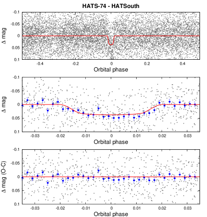
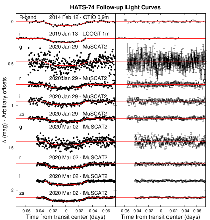
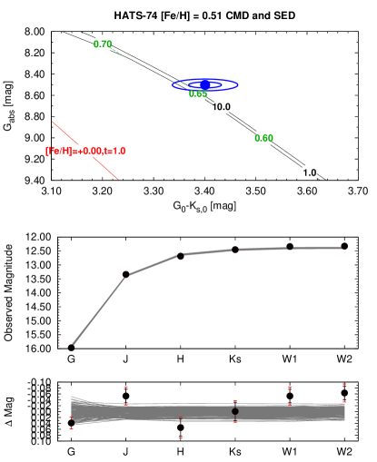
Figure 1: Observations used to confirm the transiting planet system HATS-74A, excluding data from the NASA TESS mission which are shown in Figure 5. Top Left: Phase-folded unbinned HATSouth light curve. The top panel shows the full light curve, the middle panel shows the light curve zoomed-in on the transit, and the bottom panel shows the residuals from the best-fit model zoomed-in on the transit. The solid lines show the model fits to the light curves. The dark filled circles show the light curves binned in phase with a bin size of 0.002. (Caption continued on next page.)

Figure 1: (Caption continued from previous page.) Top Right: Unbinned follow-up transit light curves corrected for instrumental trends fitted simultaneously with the transit model, which is overplotted. The dates, filters and instruments used are indicated. The residuals are shown on the right-hand-side in the same order as the original light curves. The error bars represent the photon and background shot noise, plus the readout noise. Note that these uncertainties are scaled up in the fitting procedure to achieve a reduced $\chi^{2}$ of unity, but the uncertainties shown in the plot have not been scaled. Bottom Left: Radial velocities and bisector span measurements from ESPRESSO/VLT phased with respect to the mid-transit time. The top panel shows the phased radial velocity measurements together with the best-fit model. The center-of-mass velocity has been subtracted. The middle panel shows the velocity $O\!-\!C$ residuals. The error bars include the estimated jitter, which is varied as a free parameter in the fitting. The bottom panel shows the phased bisector span measurements. Bottom Right: Color-magnitude diagram (CMD) and spectral energy distribution (SED). The top panel shows the absolute $G$ magnitude vs. the de-reddened $G-K_{S}$ color compared to theoretical isochrones (black lines) and stellar evolution tracks (green lines) from the MIST models interpolated at the best-estimate value for the metallicity of the host. The age of each isochrone is listed in black in Gyr, while the mass of each evolution track is listed in green in solar masses. The solid red lines show isochrones at higher and lower metallicities than the best-estimate value, with the metallicity and age in Gyr of each isochrone labelled on the plot. The filled blue circles show the measured reddening- and distance-corrected values from Gaia DR2 and 2MASS, while the blue lines indicate the $1\sigma$ and $2\sigma$ confidence regions, including the estimated systematic errors in the photometry. The middle panel shows the SED as measured via broadband photometry through the listed filters. Here we plot the observed magnitudes without correcting for distance or extinction. Overplotted are 200 model SEDs randomly selected from the MCMC posterior distribution produced through the global analysis (gray lines). The model makes use of the predicted absolute magnitudes in each bandpass from the MIST isochrones, the distance to the system (constrained largely via Gaia DR2) and extinction (constrained from the SED with a prior coming from the mwdust 3D Galactic extinction model). The bottom panel shows the $O\!-\!C$ residuals from the best-fit model SED. The errors listed in the catalogs for the broad-band photometry measurements are shown with black lines, while the errors including an assumed 0.02 mag systematic uncertainty, which is added in quadrature to the listed uncertainties, are shown with red lines. These latter uncertainties are what we use in the fit.

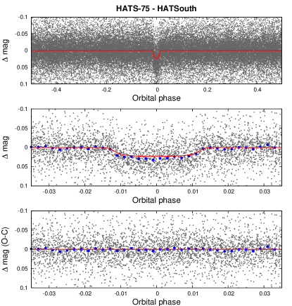
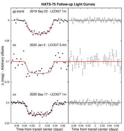
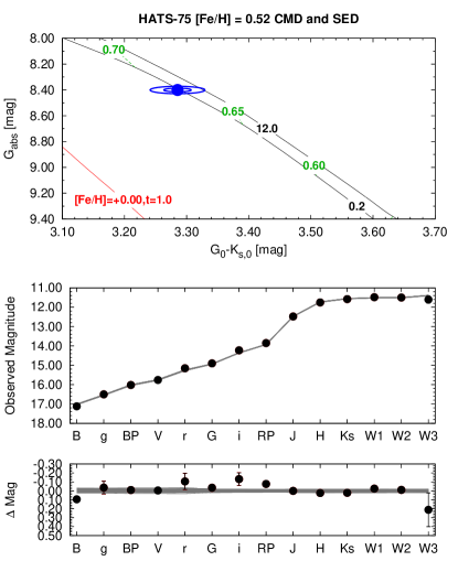
Figure 2: Same as Figure 1, here we show the observations of HATS-75 together with our best-fit model. The TESS light curve for this system is shown in Figure 6.

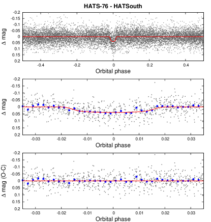
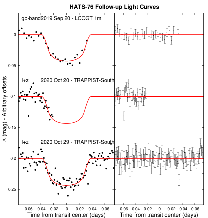
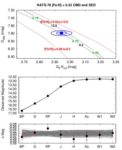
Figure 3: Same as Figure 1, here we show the observations of HATS-76 together with our best-fit model. The TESS light curve for this system is shown in Figure 7.

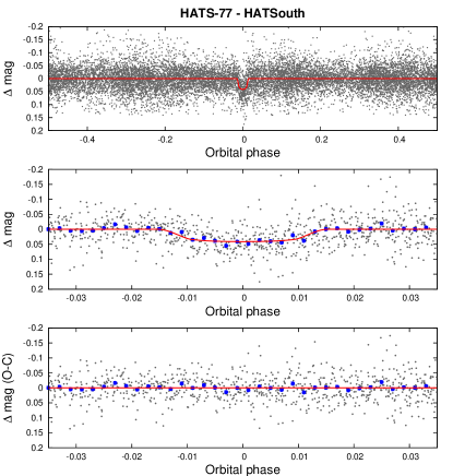
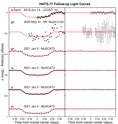
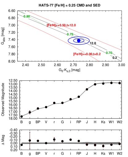
Figure 4: Same as Figure 1, here we show the observations of HATS-77 together with our best-fit model. The TESS light curve for this system is shown in Figure 8.

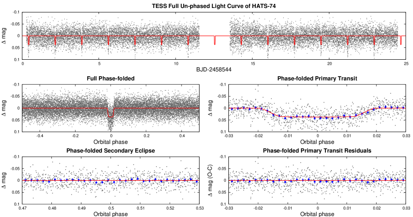
Figure 5: TESS short-cadence light curve for HATS-74A. We show the full un-phased light curve as a function of time (top), the full phase-folded light curve (middle left), the phase-folded light curve zoomed-in on the planetary transit (middle right), the phase-folded light curve zoomed-in on the secondary eclipse (bottom left), and the residuals from the best-fit model, phase-folded and zoomed-in on the planetary transit (bottom right). The solid line in each panel shows the model fit to the light curve. The dark filled circles show the light curve binned in phase with a bin size of 0.002. Other observations included in our analysis of this system are shown in Figure 1.

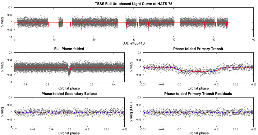
Figure 6: Similar to Figure 5, here we show the TESS short-cadence light curve for HATS-75. Other observations included in our analysis of this system are shown in Figure 2.

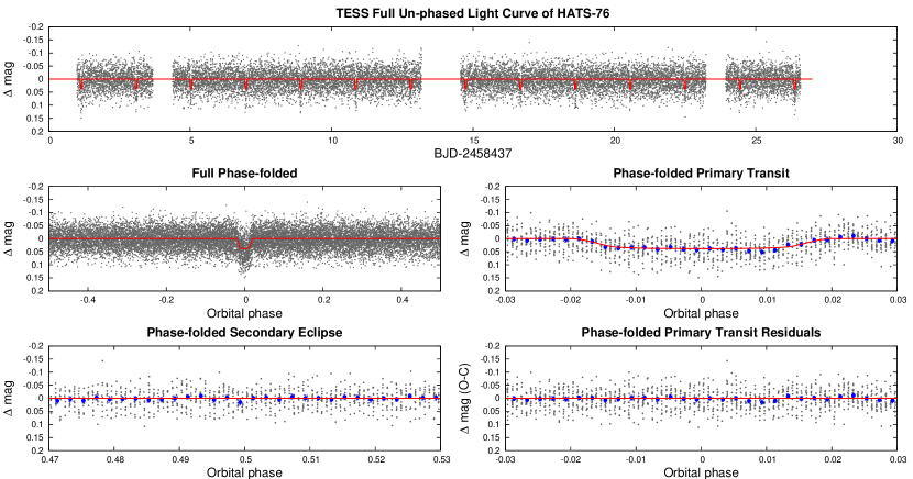
Figure 7: Similar to Figure 5, here we show the TESS short-cadence light curve for HATS-76. Other observations included in our analysis of this system are shown in Figure 3.

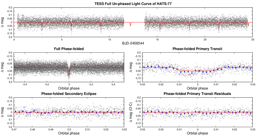
Figure 8: Similar to Figure 8, here we show the TESS short-cadence light curve for HATS-77. Other observations included in our analysis of this system are shown in Figures 4.

2.1.2 TESS

All four systems were observed by the NASA TESS mission as summarized in Table 1. Observations were carried out in short-cadence mode through the TESS Guest-Investigator program (G011214; PI Bakos) to observe HATSouth transiting planet candidates with TESS. The short-cadence observations were reduced to light curves by the NASA Science Processing Operations Center (SPOC) Pipeline at NASA Ames Research Center (Jenkins et al., 2016, 2010). Multiple threshold crossing events were identified for each target, and all four objects were selected as transiting planet candidates and assigned TESS Object of Interest (TOI) identifiers (TOI 737.01, TOI 552.01, TOI 555.01, and TOI 730.01, respectively). Each target passed all of the data validation tests conducted by the pipeline, including no discernable difference between odd and even transits, no evidence for a weak secondary event, no evidence for stronger transits in a halo aperture compared to the optimal aperture used to extract the light curve, strong evidence that the target is not a false alarm due to correlated noise, and no evidence for variations in the difference image centroid.

We obtained the SPOC PDC light curves (Stumpe et al., 2014; Smith et al., 2012) for all four objects from the Barbara A. Mikulski Archive for Space Telescopes (MAST). These light curves have been corrected for dilution from any other sources in the TESS Input Catalog (TIC; Stassun et al., 2019) that are blended with the targets in the TESS observations. The TESS light curves show clear transit signals for all four systems that are fully consistent with the transit signals detected with HATSouth as shown in Fig. 5, Fig. 6, Fig. 7, and Fig. 8. The TESS light curve data that we included in the analyses are listed in Table 2.

HATS-74A is blended in the TESS images with a $0\farcs 84$ neighbor with $\Delta G=3.183$ mag, which we denote HATS-74B in this work. The neighbor is resolved in the Gaia DR2 catalog, and was also detected in high-spatial-resolution imaging (Section 2.4). The neighbor is blended with the target in all of the time-series photometric observations which we carried out, and in all of the catalog photometry except the Gaia DR2 $G$-band measurement, and we discuss our methods for correcting these data in Section 3.1.

There are no known sources blended with either HATS-75 or HATS-76 in the TESS images down to $G\lesssim 20$ mag.

There are two sources that are within 2 pixels of HATS-77 in the TESS images, including one object with $\Delta G=1.04$ mag at a separation of $24\farcs 1$, and an object with $\Delta G=3.52$ mag at a separation of $28\farcs 8$. These two objects are fully resolved from HATS-77 in all of the other observations included in the analysis of this system.

2.1.3 Photometric Rotation Periods

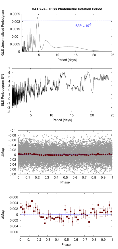
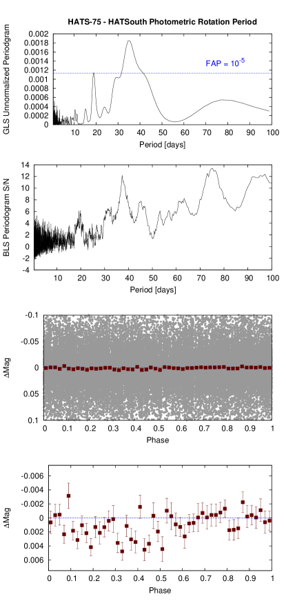
Figure 9: Detection of a $P=4.745422\pm 0.000040$ days photometric rotation period signal in the TESS light curve of HATS-74A (left) and $P=35.0435\pm 0.0017$ days signal in the HATSouth light curve of HATS-75 (right). In each case we show the following panels. Top: the Generalized Lomb-Scargle (GLS) periodogram of the light curve after subtracting the best-fit transit model. The horizontal blue line shows the bootstrap-calibrated $10^{-3}$ false alarm probability level for HATS-74A and the $10^{-5}$ false alarm probability level for HATS-75. Second from top: The Box-fitting Least Squares (BLS) periodogram of the same light curve. For HATS-74A there is a peak in the BLS periodogram at twice the period of the strongest peak in the GLS periodogram. For HATS-75 no significant peak is present in the BLS periodogram. Second from bottom: The TESS (left) and HATSouth (right) light curve phase-folded at the peak GLS period. The gray points show the individual photometric measurements, while the dark red filled squares show the observations binned in phase with a bin size of 0.02. Bottom: Same as the second from bottom, here we restrict the vertical range of the plot to better show the variation seen in the phase-binned measurements.

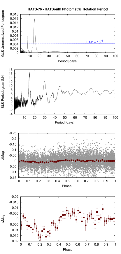
Figure 10: Similar to Fig. 9, here we show the detection of a $P=15.16063\pm 0.00048$ days photometric rotation period in the HATSouth light curve of HATS-76.

We also searched the HATSouth and TESS light curves for other periodic signals using the Generalized Lomb-Scargle method (GLS; Zechmeister & Kürster, 2009), and for additional transit signals by applying a second iteration of BLS. Both of these searches were performed on the residual light curves after subtracting the best-fit transit models. We analyzed the HATSouth and TESS light curves separately for each object.

We detect no evidence for additional variability in the HATSouth light curve of HATS-74A. The highest peak in the GLS periodogram of the HATSouth residual light curve of HATS-74A has a 95% confidence upper-limit on the semi-amplitude of 4.9 mmag, and the highest peak in the BLS periodogram has a transit depth of 16.7 mmag. The TESS light curve, however, does show evidence for a periodic signal, with a period of $4.745422\pm 0.000040$ days and a semi-amplitude of $1.86\pm 0.41$ mmag (Fig. 9, left) that we interpret as the photometric rotation period of the star. The GLS false alarm probability, calibrated using a bootstrap procedure, is $10^{-4}$. No significant additional transit signals are revealed by BLS, with the highest peak in the BLS spectrum having a transit depth of 4.3 mmag.

The GLS analysis of the HATSouth light curve of HATS-75 reveals a significant periodic signal, with a period of $35.0435\pm 0.0017$ days, semi-amplitude of $1.71\pm 0.21$ mmag, and false-alarm probability of $10^{-11}$ (Fig. 9, right). The BLS analysis identifies this same signal in the HATSouth light curve, but the morphology of the phase-folded light curve clearly indicates that this is rotational variability due to starspots, rather than a transit signal. No other transit signals are seen in the HATSouth light curve. We do not detect any variability in the residual TESS light curve of HATS-75. Note that the rotation period identified by HATSouth is too long to be detectable in the TESS data given the 27 day window for each sector, and the detrending procedures that remove low-frequency variability from the TESS light curves.

We detect a $P=15.16063\pm 0.00048$ day periodic signal in the HATSouth light curve of HATS-76 using GLS (Fig. 10). The signal has a semi-amplitude of $7.46\pm 0.66$ mmag, and a false alarm probability of $10^{-32}$. BLS also identifies this same signal, but it is clearly starspot-induced rotational variability. No other signals are identified by BLS. As for HATS-75, we do not detect the rotational variability in the TESS light curve of HATS-76 due to the long period relative to the 27 day observing window. No additional signals are detected by BLS in the TESS light curve either.

For HATS-77, no signals are identified in either the HATSouth or TESS light curves. The highest peak in the GLS periodogram of the HATSouth light curve has a 95% confidence upper-limit on its semi-amplitude of 4.1 mmag. The corresponding upper-limit for the TESS light curve is 3.1 mmag. The highest peak in the BLS spectrum of the HATSouth residuals has a depth of 13 mmag, while for the TESS residuals it is 6.0 mmag.

2.2 Spectroscopic Observations

The spectroscopic observations carried out to confirm and characterize the four transiting planet systems presented here are summarized in Table 3. The facilities used include: the Échelle spectrograph on the du Pont 2.54 m, WiFeS on the ANU 2.3 m (Dopita et al., 2007), ARCES on the ARC 3.5 m (Wang et al., 2003), FEROS on the MPG 2.2 m (Kaufer & Pasquini, 1998), ARCoIRIS on the Blanco 4 m (Abbott et al., 2016), and ESPRESSO on the VLT 8.2 m (Pepe et al., 2021). The du Pont, WiFeS, ARCES and FEROS observations were obtained only for HATS-74A, while all four systems were observed with ARCoIRIS and ESPRESSO.

A 1200 s exposure of HATS-74A was obtained with the Échelle spectrograph on the du Pont 2.54 m telescope at Las Campanas Observatory in Chile on 2011 May 18. The spectrum had a resolution of $R\equiv\lambda/\Delta\lambda=40000$, and covered the wavelength range of $3700$–$7000$ Å. Th-Ar lamp spectra were obtained before and after the observation to calibrate the wavelength scale of the science spectrum. The spectrum was extracted from the observation and analyzed following the procedure used by Jordán et al. (2014) to reduce observations from the Coralie and FEROS spectrographs. The spectrum had S/N$=7$, and thus only a low precision RV measurement was possible, and estimates of the stellar spectroscopic parameters based on this observation are unreliable.

HATS-74A was subsequently observed with the Wide Field Spectrograph (WiFeS; Dopita et al., 2007) on the ANU 2.3 m telescope at SSO. The WiFeS data were reduced and analyzed following Bayliss et al. (2013). We obtained two spectra at a resolution of $R=3000$ to determine the effective temperature, surface gravity, and metallicity of the star, while four spectra were obtained at $R=7000$ to search for large amplitude RV variations that would indicate the presence of a stellar-mass companion. The RV measurements extracted from the $R=7000$ spectra had very large uncertainties (median value of $30$ $\rm km\,s^{-1}$), and were not useful for ruling out large amplitude RV variations.

Three optical spectra of HATS-74A were obtained with the Astrophysics Research Consortium Échelle Spectrograph (ARCES; Wang et al., 2003) on the Astrophysics Research Consortium (ARC) 3.5 m telescope at Apache Point Observatory in New Mexico. The observations were performed and reduced to wavelength-calibrated spectra in the manner discussed by Brahm et al. (2015). The observations were then analyzed using the Spectral Parameter Classification program (SPC; Buchhave et al., 2012). We found that two of the spectra had S/N that were too low to yield useful measurements, while a third spectrum obtained with $S/N\sim 9$ yielded an RV measurement of $17.9\pm 0.6$ $\rm km\,s^{-1}$. The atmospheric parameters estimated from the spectra hinted at a cool surface temperature of $T_{\rm eff\star}\sim 4000$ K, but due to the low S/N, reliable surface gravity, metallicity and $v\sin{i}$ measurements could not be derived from these observations.

A single FEROS observation of HATS-74A was obtained and reduced to a wavelength-calibrated spectrum, and RV and BS measurements using the CERES software package (Brahm et al., 2017a). The CERES package produced a high effective temperature of $7000$ K and low metallicity of $\rm[Fe/H]=-2.0$ dex, which we find to often be the case for M dwarfs with temperatures below the $T_{\rm eff\star}=4000$ K lower limit of the model spectra used for cross-correlation by the package. The measurements RV of $15.87\pm 0.11$ $\rm km\,s^{-1}$ is consistent with the higher-precision RV measurements of the system obtained with ESPRESSO.

Because all four objects have surface temperatures that are too low to apply the ZASPE package of (Brahm et al., 2017b), we obtained near-infrared spectra of all four systems using the “Astronomy Research using the Cornell Infra Red Imaging Spectrograph” (ARCoIRIS) instrument on the Blanco 4 m at CTIO (Abbott et al., 2016). ARCoIRIS is a fixed slit spectrograph. It reaches a resolution of R$\sim$3500 over a large wavelength range from 0.80 to 2.47 microns by cross-dispersing the reflected grating light. For each science frame, we used the Fowler readout mode and took subsequent CuHeAr lamp spectra. We interleaved telluric standard star observations in the course of the night, matching the spectral type A0V and close in air mass. All stars were observed in an ABBA pattern. We analyzed the raw ARCoIRIS frames using SpexTool (Cushing et al., 2004a; Vacca et al., 2003), obtaining wavelength calibrated and telluric corrected spectra. Given the mixed cloud conditions, we did not attempt to flux calibrate the spectra. Stellar atmospheric parameters were obtained by downgrading our spectra to match the IRTF/SpeX resolution and applying the procedure described in Newton et al. (2014, 2015). These are the atmospheric parameters that we adopt for the joint analysis discussion in Section 3.1. We also obtained ARCoIRIS spectra of two known M-dwarfs (namely GJ176 and GJ205) for which we applied the same procedure. The ARCoIRIS spectra for our targets, along with IRTF/SpeX and ARCoIRIS spectra for standards, are shown in Figure 11.

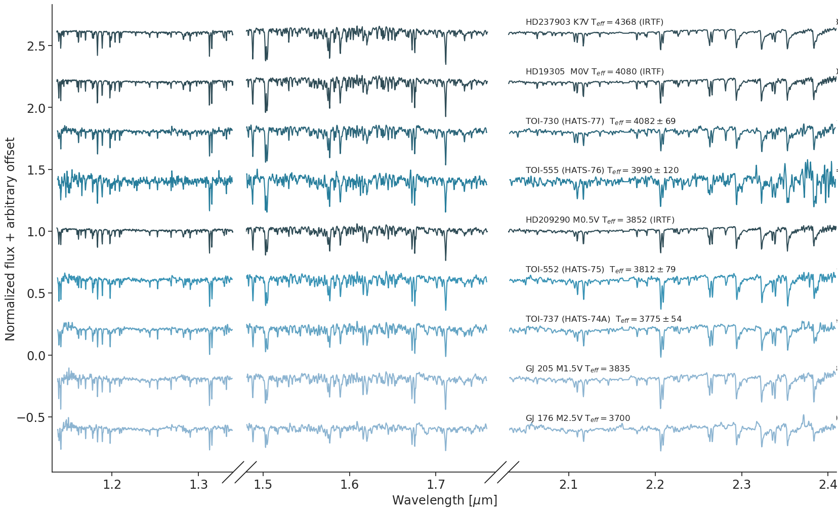
Figure 11: ARCoIRIS spectra for our targets, along with IRTF/SpeX and ArcoIRIS spectra for M dwarfs with known stellar atmospheric parameters. The ARCoIRIS spectra have been degraded to the resolution of IRTF/SpeX for this figure. The effective temperatures derived using the procedure of Newton et al. (2014, 2015) are indicated over the K band spectra.

In order to detect the radial velocity variation of each star due to the transiting companions, and thereby determine the mass of each transiting companion, and confirm these as transiting planet systems, we obtained VLT 8.2 m/ESPRESSO observations of all four objects. A large telescope was needed to perform these observations due to the faintness, in optical bandpasses, of the host stars. The observations were carried out through the queue service mode between 2019 September and 2019 December. We used an exposure time of 1800 s for all observations, and obtained five exposures each for HATS-74A, HATS-75 and HATS-77, and four exposures for HATS-76. The observing and reduction procedures were the same as those discussed in (Bakos et al., 2020), making use of version 2.0.0 of the ESPRESSO pipeline in the ESO Reflex environment (Freudling et al., 2013) to produce high-precision RVs and bisector span measurements via cross-correlation with an M2 spectra mask. During the observations, the target was placed on fiber A, while fiber B pointed to the sky for a simultaneous monitoring of the sky. For all four objects the resulting RVs showed clear variations in phase with the transit ephemerides, and consistent with Keplerian orbital variations due to transiting planets. The phase-folded observations are shown in Fig. 1, Fig. 2, Fig. 3, and Fig. 4, while the radial velocity and bisector span data are made available in Table 5.

Table 1: Summary of photometric observations

Instrument/Field	Date(s)	# Images	Cadence	Filter	Precision
			(sec)		(mmag)
HATS-74A
HS-1/G563	2010 Jan–2010 Aug	3875	277	$r$	44.4
HS-3/G563	2010 Jan–2010 Aug	5197	281	$r$	46.0
HS-5/G563	2010 Jan–2010 Aug	636	271	$r$	41.9
TESS/Sector 9	2019 Mar 1–25	15918	120	$T$	24.8
CTIO 0.9 m	2014 Feb 12	74	240	$R$	7.5
LCO 1 m/Sinistro	2019 Jun 13	50	206	$i$	4.6
TCS 1.5 m/MuSCAT2	2020 Jan 29	371	30	$g$	59.0
TCS 1.5 m/MuSCAT2	2020 Jan 29	189	60	$r$	16.6
TCS 1.5 m/MuSCAT2	2020 Jan 29	189	60	$i$	16.5
TCS 1.5 m/MuSCAT2	2020 Jan 29	189	60	$z_{S}$	10.7
TSC 1.5 m/MuSCAT2	2020 Mar 2	384	30	$g$	33.8
TCS 1.5 m/MuSCAT2	2020 Mar 2	196	60	$r$	9.7
TCS 1.5 m/MuSCAT2	2020 Mar 2	195	60	$i$	7.0
TCS 1.5 m/MuSCAT2	2020 Mar 2	195	60	$z_{S}$	5.5
HATS-75
HS-1/G548.focus	2014 Sep–2015 Apr	1677	1071	$r$	53.2
HS-2/G548.focus	2014 Jun–2015 Mar	2011	1209	$r$	52.6
HS-3/G548.focus	2014 Sep–2015 Mar	1486	1217	$r$	52.4
HS-4/G548.focus	2014 Jun–2015 Mar	1702	1222	$r$	51.0
HS-5/G548.focus	2014 Sep–2015 Mar	1381	1232	$r$	52.1
HS-6/G548.focus	2014 Jul–2015 Mar	1672	1200	$r$	51.5
HS-1/G548	2014 Sep–2015 Apr	6547	287	$r$	28.5
HS-2/G548	2014 Jun–2015 Apr	7590	348	$r$	28.2
HS-3/G548	2014 Sep–2015 Mar	5284	352	$r$	27.4
HS-4/G548	2014 Jun–2015 Mar	5976	352	$r$	26.9
HS-5/G548	2014 Sep–2015 Mar	4945	359	$r$	31.6
HS-6/G548	2014 Jul–2015 Mar	5956	351	$r$	30.0
TESS/Sector 4	2018 Oct–Nov	14368	120	$T$	13.9
TESS/Sector 5	2018 Nov–Dec	16376	120	$T$	13.1
LCO 1 m/Sinistro	2019 Sep 23	44	276	$g^{\prime}$	2.8
LCO 0.4 m	2020 Jan 2	38	314	$z_{S}$	11.6
LCO 1 m/Sinistro	2020 Sep 17	83	181	$z_{S}$	2.6
HATS-76
HS-1/G597	2014 Jan–2014 Mar	1228	286	$r$	38.6
HS-3/G597	2013 Sep–2014 Feb	4540	285	$r$	44.4
HS-5/G597	2013 Sep–2014 Mar	4915	278	$r$	44.7
TESS/Sector 5	2018 Nov–Dec	16362	120	$T$	36.1
LCO 1 m/Sinistro	2019 Sep 20	44	327	$g^{\prime}$	4.9
TRAPPIST-South	2020 Oct 20	48	130	$I+z$	9.1
TRAPPIST-South	2020 Oct 29	138	130	$I+z$	10.2
HATS-77
HS-1/G607	2011 Jan–2012 Jun	6703	289	$r$	43.3
HS-3/G607	2011 Jan–2012 Jun	3179	294	$r$	48.4
HS-5/G607	2011 Jan–2012 Jun	2544	288	$r$	44.6
TESS/Sector 9	2019 Mar 1–25	15726	120	$T$	39.4
LCO 1 m/Sinistro	2019 Jun 14	55	147	$i^{\prime}$	5.9
Mt. Stuart 0.3 m	2020 May 31	66	191	$g^{\prime}$	32.8
LCO 2 m/MuSCAT3	2021 Jan 5	44	404	$g$	2.2
LCO 2 m/MuSCAT3	2021 Jan 5	73	244	$r$	1.1
LCO 2 m/MuSCAT3	2021 Jan 5	92	194	$i$	1.2
LCO 2 m/MuSCAT3	2021 Jan 5	44	404	$z_{S}$	1.5

Table 2: Light curve data for HATS-74A, HATS-75, HATS-76, and HATS-77.

Object	BJD	Mag	$\sigma_{\rm Mag}$	Mag(orig)	Filter	Instrument
HATS-74	$2455254.76774$	$-0.08602$	$0.05337$	$\cdots$	$r$	HS
HATS-74	$2455322.31035$	$0.04862$	$0.03805$	$\cdots$	$r$	HS
HATS-74	$2455280.74579$	$-0.01962$	$0.02762$	$\cdots$	$r$	HS
HATS-74	$2455379.46209$	$0.05838$	$0.04105$	$\cdots$	$r$	HS
HATS-74	$2455263.42771$	$0.01115$	$0.03608$	$\cdots$	$r$	HS
HATS-74	$2455294.60127$	$0.03434$	$0.03152$	$\cdots$	$r$	HS
HATS-74	$2455247.84123$	$-0.02098$	$0.02971$	$\cdots$	$r$	HS
HATS-74	$2455289.40588$	$-0.00697$	$0.08795$	$\cdots$	$r$	HS
HATS-74	$2455374.26713$	$0.06199$	$0.04867$	$\cdots$	$r$	HS
HATS-74	$2455327.50711$	$0.01042$	$0.06350$	$\cdots$	$r$	HS

Note. — This table is available in a machine-readable form in the online journal. A portion is shown here for guidance regarding its form and content.

Table 3: Summary of spectroscopy observations.

Instrument	UT Date(s)	# Spec.	Res.	S/N Range	$\gamma_{\rm RV}$	RV Precision
			$\Delta\lambda$/$\lambda$/1000		($\rm km\,s^{-1}$)	($\rm m\,s^{-1}$)
HATS-74A
du Pont 2.54 m/Echelle	2011 May 18	1	30	7	$5.4$	$\sim 10000$
ANU 2.3 m/WiFeS	2011 Jun 6	2	3	43–46	$\cdots$	$\cdots$
ARC 3.5 m/ARCES	2012 Apr–2013 Feb	3	31.5	7–9	$17.9$	$\sim 1000$
ANU 2.3 m/WiFeS	2013 Mar–Apr	4	7	$\cdots$	$8.8$	$30000$
MPG 2.2 m/FEROS	2013 May 12	1	48	14	15.868	100
Blanco 4 m/ARCoIRIS	2017 Jun 8–9	2	3.5	120	$\cdots$	$\cdots$
VLT 8.2 m/ESPRESSO	2019 Dec 26–31	5	140	$\cdots$	15.853	11.0
HATS-75
Blanco 4 m/ARCoIRIS	2017 Dec 2	1	3.5	90	$\cdots$	$\cdots$
VLT 8.2 m/ESPRESSO	2019 Sep–Oct	5	140	$\cdots$	39.995	2.9
HATS-76
Blanco 4 m/ARCoIRIS	2017 Dec 2	1	3.5	40	$\cdots$	$\cdots$
VLT 8.2 m/ESPRESSO	2019 Sep–Oct	4	140	$\cdots$	8.601	35.7
HATS-77
Blanco 4 m/ARCoIRIS	2017 Jun 8–9	2	3.5	70–100	$\cdots$	$\cdots$
VLT 8.2 m/ESPRESSO	2019 Dec 1–27	5	140	$\cdots$	-7.759	25.0

2.3 Photometric follow-up observations

We obtained additional follow-up time-series photometry for each system using larger 0.3 m–2 m ground-based telescopes to obtain higher photometric-precision light curves from higher-spatial-resolution images than those available from HATSouth or TESS. As summarized in Table 1, the facilities that we made use of for this purpose include: the imager on the CTIO 0.9 m (Subasavage et al., 2010), the imagers on the Las Cumbres Observatory (Brown et al., 2013) 0.4 m network (LCO 0.4 m), the Sinistro imagers on the Las Cumbres Observatory 1 m network (LCO 1 m), the MuSCAT2 imager (Narita et al., 2019) on the 1.5 m Telescopio Carlos Sanchez (TCS) at Teide Observatory, the MuSCAT3 imager (Narita et al., 2020) at LCO’s 2 m telescope at Haleakala Observatory, and the imager on the Mt. Stuart 0.3 m telescope near Dunedin, New Zealand. The CTIO 0.9 m observations were carried out by the HATSouth team, while the other observations were carried out by members of the TESS Follow-up Observing Program (TFOP; Collins et al., 2018), and were made available to the community through the ExoFOP-TESS portal. For the TFOP observations, we used the TESS Transit Finder, which is a customized version of the Tapir software package (Jensen, 2013), to schedule the observations, and the photometric data were extracted using AstroImageJ (Collins et al., 2017).

2.4 Search for Resolved Stellar Companions

High-spatial-resolution images were obtained for all four objects by members of TFOP, and made available on ExoFOP-TESS as part of the standard process for vetting transit candidates and properly accounting for transit dilution that may be caused by the presence of stellar companions (Ciardi et al., 2015; Schlieder et al., 2021). Optical speckle imaging was carried out at 562 nm and 832 nm with the twin Zorro and ’Alopeke imagers (Scott et al. 2021, in press) mounted on the Gemini 8 m South and North telescopes, respectively. Near-infrared (NIR) adaptive optics (AO) imaging in Br$\gamma$ and the $J$-band was performed with the NIRC2 instrument on the Keck 2 m for HATS-74A, and in the $K_{s}$-band with the NaCo instrument on the VLT 8 m for HATS-75. Finally, $J$ and $K_{s}$-band imaging of HATS-77 was obtained with WHIRC on the ARC 3.5 m. The observations with this latter instrument were gathered by the HATSouth team before the TESS mission. The optical and near-infrared techniques complement each other in terms of resolution and sensitivity to yield a more complete picture of the presence of near-by and (possibly) bound companions, with the optical speckle typically have better resolution and the NIR AO having better sensitivity. The various observations are described below.

HATS-76 and HATS-77 were observed with Zorro, and HATS-74A and HATS-75 were observed with ’Alopeke. The two instruments provide simultaneous speckle imaging in two bands (562nm and 832 nm) with output data products including a reconstructed image with robust contrast limits on companion detections (e.g., Howell et al., 2016). Images were collected and subjected to Fourier analysis in our standard reduction pipeline (see Howell et al., 2011). We find that all four targets are single stars to within the contrast achieved by the observations (4-5 magnitudes) from the diffraction limit (20 mas) out to 1.2”. At the distances of these HATS stars ($d=195$ to 414 pc) these angular limits correspond to spatial limits of 4-8 AU out to 230–500 AU. We note that AO imaging reveals a companion to HATS-74A at $0\farcs 844$ which was not immediately apparent in the ’Alopeke data.

The NaCo (Lenzen et al., 2003; Rousset et al., 2003) data were collected in a nine-point grid dither pattern, with the star position moved 2$\arcsec$ for each exposure. We ensured the star was within the upper left quadrant of the detector for all images, since other quadrants of the detector suffer from light- and dark- column striping in the images. We collected 9 individual frames, each with exposure time 75 s, using the Ks filter. The dither pattern allows for a sky background frame to be constructed from a median-combination of the science frames themselves. We reduced the raw data using a custom code, which performs badpixel and flatfield correction, subtracts the sky background, aligns the stellar position between images and finally co-adds the nine individual frames. We visually inspected images to search for companions, and did not find companions anywhere in the field of view, which extends to at least 4.9$\arcsec$ from the star in all directions. To quantify the sensitivity of the final image, we injected fake companions into the data cube at a range of separations and position angles. We retrieved these fake companions, and measured the S/N of each fake companion. We then scaled the flux of the fake companions, such that they could be retrieved at 5$\sigma$. Finally, the sensitivity was averaged over position angle. We are sensitive to companions 3.7 mag fainter than the host beyond 400mas, and to companions 5 mag fainter than the host in the background-limited regime beyond  700 mas. Our NaCo detection limits as a function of radius for HATS-75 are shown in Figure 13.

HATS-74A was observed with the NIRC2 instrument on Keck-II behind the natural guide star AO system (Wizinowich et al., 2000). The observations were made on 2019 Jun 10 UT in the standard 3-point dither pattern that is used with NIRC2 to avoid the left lower quadrant of the detector which is typically noisier than the other three quadrants. The dither pattern step size was $3\arcsec$ and was repeated twice, with each dither offset from the previous dither by $0.5\arcsec$. The camera was in the narrow-angle mode with a full field of view of $\sim 10\arcsec$ and a pixel scale of approximately $0.0099442\arcsec$ per pixel. The observations were made in the narrow-band $Br\gamma$ filter $(\lambda_{o}=2.1686;\Delta\lambda=0.0326\,\mu$m) and the narrow-band $J_{cont}$ filter ($\lambda_{o}=1.2132;\Delta\lambda=0.0198\,\mu$m), each with an integration time of 60 seconds with one coadd per frame for a total of 540 seconds on target per filter.

The AO data were processed and analyzed with a custom set of IDL tools. The science frames were flat-fielded and sky-subtracted. The flat fields were generated from a median average of dark subtracted flats taken on-sky, and the flats were normalized such that the median value of the flats is unity. Sky frames were generated from the median average of the 9 dithered science frames; each science image was then sky-subtracted and flat-fielded. The reduced science frames were combined into a single combined image using a intra-pixel interpolation that conserves flux, shifts the individual dithered frames by the appropriate fractional pixels, and median-coadds the frames. The final resolution of the combined dithers was determined from the full-width half-maximum of the point spread function; 0.064″ and 0.121″ for $Br\gamma$ and $J_{cont}$ observations, respectively. The sensitivities of the final combined AO image were determined by injecting simulated sources azimuthally around the primary target every $20^{\circ}$ at separations of integer multiples of the central source’s FWHM (Furlan et al., 2017). The brightness of each injected source was scaled until standard aperture photometry detected it with $5\sigma$ significance. The resulting brightness of the injected sources relative to the target set the contrast limits at that injection location. The final $5\sigma$ limit at each separation was determined from the average of all of the determined limits at that separation and the uncertainty on the limit was set by the rms dispersion of the azimuthal slices at a given radial distance.

Additional imaging results are available for all four objects from Gaia DR2 (Gaia Collaboration et al., 2018), which is sensitive to neighbors with $G\lesssim 20$ mag down to a limiting resolution of $\sim 1\arcsec$ (e.g., Ziegler et al., 2018).

Based on the NIRC2 observations we find that HATS-74A has a $0\farcs 844\pm 0\farcs 0014$ neighbor at a position angle of 46^∘ east of north. The neighbor has magnitudes, relative to HATS-74A, of $\Delta Br\gamma=2.615\pm 0.013$ mag and $\Delta J=2.642\pm 0.030$ mag (Fig. 12). The neighbor is not obviously apparent in the ’Alopeke images, however (Fig. 12). Finally, the neighbor is also listed in the Gaia DR2 catalog with a projected separation of $0\farcs 84$ and a relative magnitude of $\Delta G=3.1830\pm 0.0049$ mag. The neighbor has a parallax of $3.80\pm 0.63$ mas and a proper motion of $\mu_{\rm R.A.}=-41.4\pm 1.4$ $\rm mas\,yr^{-1}$, and $\mu_{\rm Dec.}=42.6\pm 1.5$ $\rm mas\,yr^{-1}$, which are consistent with the values listed for HATS-74A ($\pi=3.425\pm 0.042$ mas, $\mu_{\rm R.A.}=-38.86\pm 0.12$ $\rm mas\,yr^{-1}$, and $\mu_{\rm Dec.}=39.679\pm 0.077$ $\rm mas\,yr^{-1}$), indicating that the neighbor is very likely a bound companion to HATS-74A, and we henceforth refer to it has HATS-74B. Given the distance to HATS-74A (Table 6), the measured angular separation between HATS-74A and HATS-74B corresponds to a projected physical separation of $238.4\pm 3.9$ AU. Assuming HATS-74B is a main sequence companion to HATS-74A with the same age, metallicity, distance and extinction, then from the blend analysis that we discuss in Section 3.2 we find that HATS-74B has a stellar mass of $0.2284\pm 0.0078$ $M_{\sun}$.

No neighbors are detected for the other three systems, HATS-75, HATS-76, or HATS-77. Figures-13–15 show contrast limits on any resolved neighbors that are derived based on the high-resolution imaging that we have reported for these three objects.

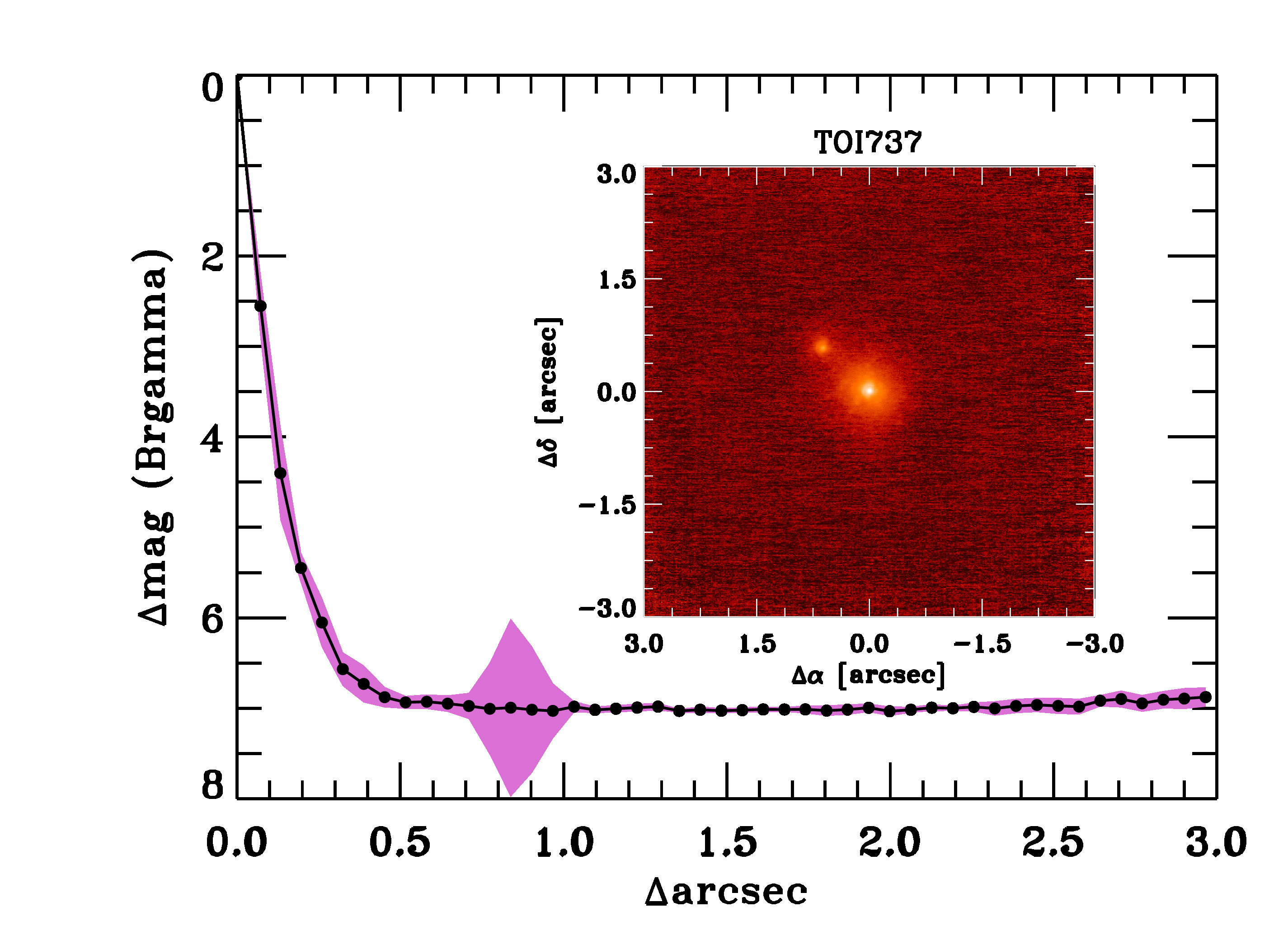
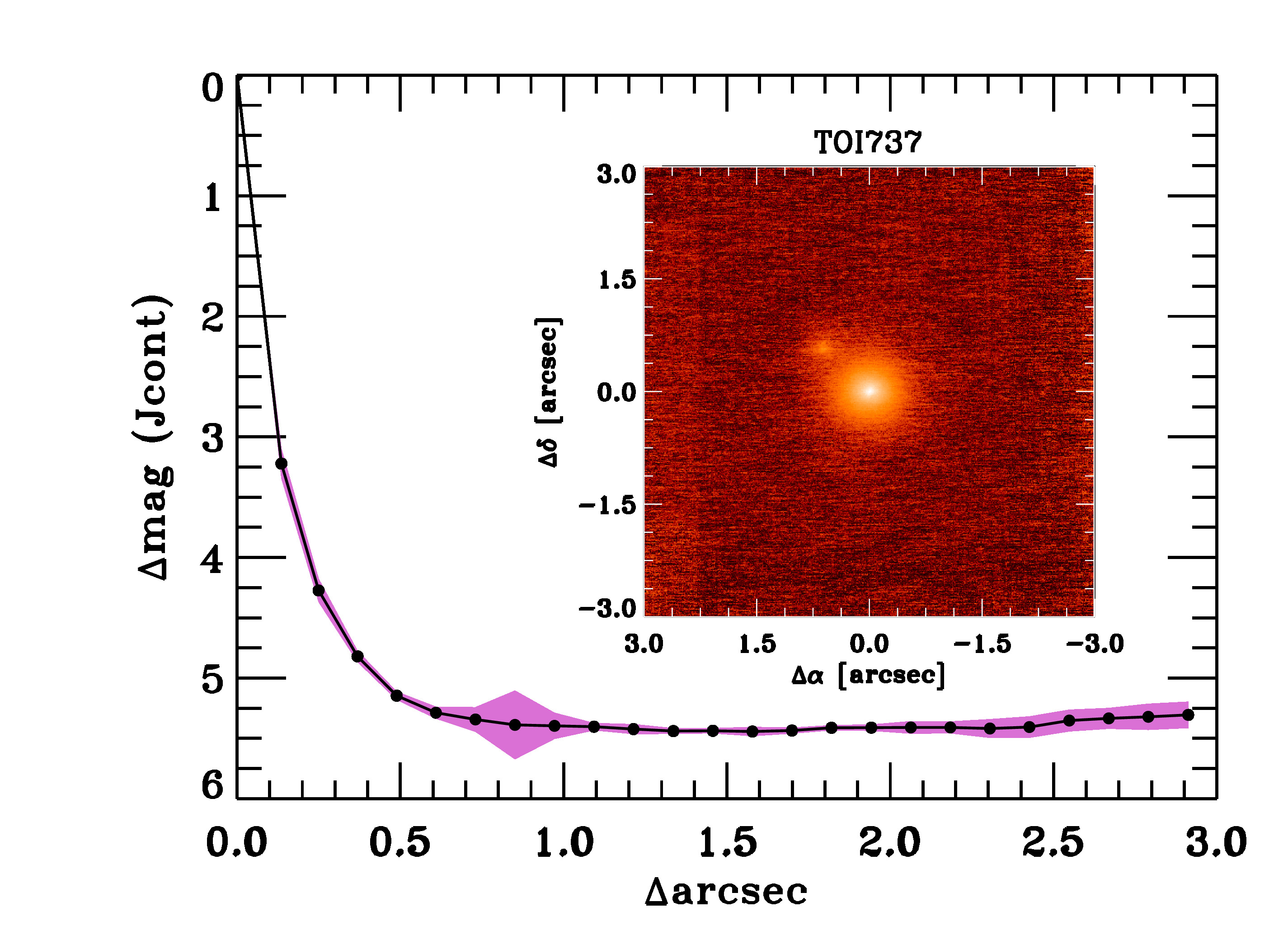
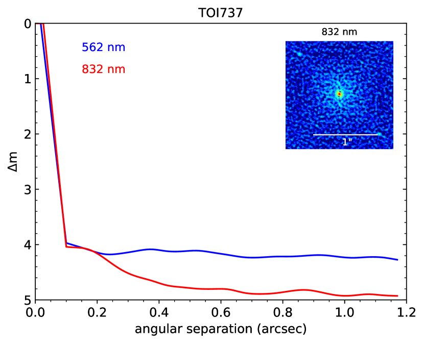
Figure 12: (Top) High-resolution images in Br$\gamma$ (left) and $J$-continuum (middle) and associated contrast curve for HATS-74A (TOI 737) from Keck-2/NIRC2. The $0\farcs 844$ neighbor HATS-74B is apparent in these images. (Bottom) Contrast curves at 562 nm and 832 nm from the ’Alopeke/Gemini 8 m observations of HATS-74A. The 832 nm image is also shown in the inset.

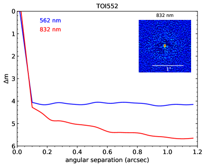
Figure 13: (Left) Contrast curves for HATS-75 (TOI 552) derived from high-resolution images at 562 nm and 832 nm obtained with ’Alopeke/Gemini 8 m. The 832 nm image is also shown in the inset. (right) Contrast curve for HATS-75 derived from high-resolution $K_{s}$-band imaging with NaCo/VLT.

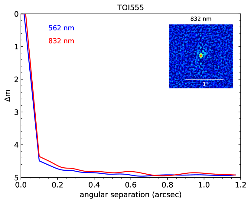
Figure 14: Contrast curves for HATS-76 (TOI 555) derived from high-resolution images at 562 nm and 832 nm obtained with Zorro/Gemini 8 m. The 832 nm image is also shown in the inset.

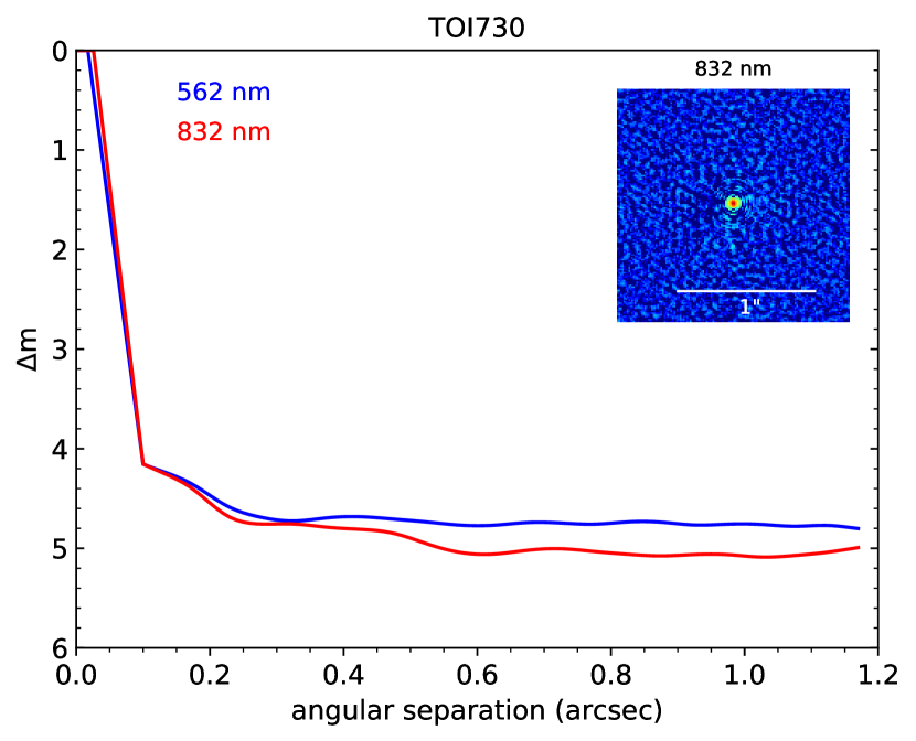
Figure 15: Contrast curves for HATS-77 (TOI 730) derived from high-resolution images at 562 nm and 832 nm obtained with Zorro/Gemini 8 m. The 832 nm image is also shown in the inset.

3 Analysis

3.1 Transiting Planet Modelling

We perform a global fit to the light curves, radial velocities, spectroscopically measured stellar atmospheric parameters, broad-band photometry, and parallax from Gaia DR2, using the methods described in Hartman et al. (2019), with modifications as summarized most recently by Bakos et al. (2018). The fit is carried out using a modified version of the lfit program which is included in the fitsh software package (Pál, 2012). The light curves are modelled using the Mandel & Agol (2002) transit model with quadratic limb-darkening. The limb darkening coefficients are allowed to vary in the fit. We place Gaussian prior constraints on the limb darkening coefficients using the tables of Claret et al. (2012, 2013) and Claret (2018) and assume a prior uncertainty of $0.2$ for each coefficient.

We include in the model several parameters for the physical and observed properties of the host star, including the effective temperature, the metallicity, the distance modulus, and the $V$-band extinction $A_{V}$. These parameters are, in turn, constrained by the observed spectroscopic stellar atmospheric parameters (as measured in Section 2.2), the photometry, and the parallax. Together with the parameters used to describe the transit and radial velocity observations, these parameters are sufficient to determine the bulk physical properties of the stars and their transiting planets. We fit the data using two different methods to relate the stellar mass to the stellar radius, metallicity and luminosity: (1) an empirical method which uses the stellar mean density measured from the transit and radial velocity observations to determine the stellar mass from the stellar radius, which is itself inferred from the effective temperature and luminosity (this method is similar to that of, e.g., Stassun et al., 2017), and (2) using version 1.2 of the MIST stellar evolution models (Dotter, 2016; Choi et al., 2016; Paxton et al., 2011, 2013, 2015) to impose an additional constraint on the stellar relations that is typically tighter than the observed constraint on the stellar mean density. Note that here we take a different approach from prior HATSouth discovery papers which generally made use of the PARSEC stellar evolution models (Marigo et al., 2017) instead. In each case, we assume both the orbital eccentricity is zero and allow the eccentricity to be a free parameter.

A Differential Evolution Markov Chain Monte Carlo (DEMCMC) procedure is used to sample the posterior parameter distribution. See Hartman et al. (2019) for a full list of the parameters that we vary, and their assumed priors. The fit includes the optical broad-band photometry from Gaia DR2 and APASS, NIR photometry from 2MASS, and IR photometry from WISE. For WISE we exclude the W4 band for all systems as none of the objects were detected in that bandpass, while for HATS-74A, HATS-76, and HATS-77 we also exclude the W3 bands. These observations, together with the stellar atmospheric parameters, the parallax, and the reddening, constrain the luminosity of the star. To model the reddening, we assume a $R_{V}=3.1$ Cardelli et al. (1989) dust law parameterized by $A_{V}$, and use the mwdust 3D Galactic extinction model (Bovy et al., 2016) to place a prior constraint on its value.

For HATS-74A we excluded the Gaia DR2 $BP$ and $RP$ measurements as we expect these to be contaminated in a non-trivial way from blending with the $0\farcs 8$ neighbor HATS-74B (Section 2.4). For the $J$, $H$, $K_{S}$, $W1$ and $W2$ bandpasses HATS-74A and HATS-74B are completely blended. In these cases we estimated $\Delta{\rm mag}$ values in each bandpass from the MIST isochrones assuming a $0.23$ $M_{\sun}$ stellar mass for the companion, and that its age, metallicity, distance and redenning are the same as those for HATS-74A, determined in an initial iteration of the analysis. These $\Delta{\rm mag}$ values, which are given in the footnotes to Table 4, were then used to subtract the flux from HATS-74B from each bandpass measurement. The corrected magnitudes are then included in the fit, and are what we list for HATS-74A in Table 4.

We find that for all four transiting planet systems the orbits are consistent with being circular when the eccentricities are varied, and that the stellar parameters are more robustly constrained when imposing the stellar evolution model constraints. We therefore choose to adopt the parameters that stem from fixing the orbit to be circular, and imposing the stellar evolution models as a constraint on the stellar physical parameters.

The best-fit models are compared to the various observational data for the four transiting planet systems in Figures 1–8. The adopted stellar parameters derived from the analysis are listed in Table 6, while the adopted planetary parameters are listed in Table 7. We also list in Table 7 the 95% confidence upper limit on the eccentricity that comes from allowing the eccentricity to vary in the fit.

3.2 Stellar Blend Modelling

We performed a blend modelling of each system following the procedure described in Hartman et al. (2019). In summary, our blend modelling attempts to fit all of the observations excepting the radial velocity data using various combinations of stars with parameters constrained by the MIST models. We find that for HATS-76 a model consisting of a single star with a transiting planet provides a better fit (a greater likelihood or equivalently lower $\chi^{2}$) to the light curves, spectroscopic stellar atmospheric parameters, broad-band catalog photometry, and astrometric parallax measurements than the best-fit blended stellar eclipsing binary models. The blended stellar eclipsing binary models involve more free parameters than the transiting planet model, and thus can be rejected on the grounds that they are both poorer-fitting and higher complexity models. However, for HATS-75, and HATS-77, we find that blends between a foreground star and a background eclipsing binary provide somewhat better fits to these data than do models consisting of a single star with a transiting planet. In these cases, comparably good fits to the data can be found for models consisting of a star with both a transiting planet and an unresolved stellar companion. For all three systems, the improvement in $\chi^{2}$ for the blends can be attributed to the increased number of free parameters that are included in these more complicated models. For these two systems we simulated radial velocities for the model blend scenarios by simulating composite cross-correlation functions. We find that for HATS-75 the blend scenarios that we considered would produce radial velocity variations in excess of $600$ $\rm m\,s^{-1}$ that do not vary sinusoidally in phase with the transit ephemeris. This is in contrast to the observed radial velocity variation that have $K=99.2\pm 7.9$ $\rm m\,s^{-1}$ and that are in phase with the transit ephemeris. Similarly, for HATS-77 we find that the simulated blended eclipsing binary radial velocities do not vary sinusoidally in phase with the ephemeris, and that the scatter is in excess of 1 $\rm km\,s^{-1}$, compared to the observed radial velocity variation with $K=562\pm 15$ $\rm m\,s^{-1}$ in phase with the transits. We conclude therefore that the blended eclipsing binary scenarios that might reproduce the photometric data for HATS-75 and HATS-77 can be ruled out on the grounds that they do not reproduce the radial velocity observations. We therefore consider HATS-75 and HATS-77, like HATS-76, to be confirmed transiting planet systems.

For HATS-74A, with its known resolved neighbor (Section 2.4), we considered four scenarios: (1) a transiting planet around the brighter source, with the fainter source being a bound companion; (2) a transiting planet around the fainter source, with the brighter source being a bound stellar companion; (3) the brighter source being a blend between a bright foreground star and a background stellar eclipsing binary, and the fainter source being unrelated to either the foreground star or the eclipsing binary; (4) the brighter source being a foreground star, and the fainter source being a background stellar eclipsing binary. In all cases we assume the 2MASS $J$, $H$, $K_{S}$, and the $W1$ and $W2$ photometry is blended between the two known sources, while $\Delta J$ from the NIRC2 observations, and $G$ and the parallax values from Gaia DR2 are unblended. The mass of both resolved stars are varied in the fits. They are assumed either to have the same age, distance, metallicity, and extinction, or independent values for these, depending on the scenario considered.

We find that scenarios (2) and (4) for HATS-74A do not fit the data included in the modelling, and can be therefore easily ruled out. Scenario (3) provides a somewhat better fit to the data than scenario (1), however, it uses seven extra parameters and the improvement in $\chi^{2}$ can be fully attributed to the additional model complexity. As an additional check on scenario (3) we simulated radial velocity observations for 1000 blend scenarios drawn randomly from the posterior chain. For each draw from the chain we simulated the radial velocity observations in two ways: (a) assuming the resolved star is also resolved in the ESPRESSO observations; and (b) assuming it is not resolved in the ESPRESSO observations. We find that in all cases the simulated radial velocities show much larger variations (well in excess of 1 $\rm km\,s^{-1}$) compared to the observed ones ($K=346\pm 34$ $\rm m\,s^{-1}$), and, moreover, they do not exhibit a clean, in-phase Keplerian orbital variation. We conclude therefore that scenario (3) is not consistent with all of the observations, and confirm that HATS-74A is a transiting planet system, with a resolved binary star companion. The modelling carried out for scenario (1) yields a mass for the binary star companion of $0.2284\pm 0.0078$ $M_{\sun}$, which we adopt in Table 6.

For HATS-75, HATS-76 and HATS-77 we place limits on the presence of any unresolved binary star companions based on this modelling which we also list in Table 6. Additionally, we note that any such companion would need to satisfy the contrast limits based on the null detection of companions in the high resolution imaging discussed in Section 2.4. Finally, we note that there is no evidence of correlation of the bisector span measurements with orbital phase for any of the systems.

4 Discussion

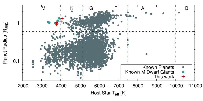
Figure 16: Planetary radius versus stellar effective temperature $T_{\rm eff}$ for confirmed transiting exoplanets. The dotted vertical lines indicate the $T_{\rm eff}$ values that roughly separate the host star spectral types as indicated on top, while the horizontal line at $R=0.6R_{J}$ indicates the separation between giant and smaller planets. Different symbols are used to plot known giants around M dwarfs and the discoveries presented in this work as indicated in the legend. Data were downloaded from the NASA Exoplanet Archive on May 13 2021.

We have presented in this work the discovery of four giant planets hosted by early M and late K dwarf stars. We place these discoveries in the context of known planets in Figure 16, where we plot radius versus effective temperature of the host star for all exoplanets that have these quantities measured. It is apparent in this figure that the discoveries presented in this work add significantly to the number of known transiting giant planets hosted by stars with effective temperatures $T_{\rm eff}\lesssim 4000$ K. As stated in the introduction, these kinds of systems are intrinsically rare and observationally challenging to confirm due to the faintness of the host stars. To confirm these exoplanet, we need high resolution stable spectrographs mounted on large aperture telescopes. In this work we used ESPRESSO mounted on the VLT in order to confirm and measure the masses for our discoveries. Also noteworthy in terms of the required discovery resources is the fact that these systems were first uncovered as candidates by the HATSouth survey, and observed by the TESS mission in high cadence by virtue of their nature as candidates from a ground-based survey.

In Figure 17 we plot out discoveries in the mass-radius plane along with other confirmed planets with measured masses and radii. We color-code in the figure the equilibrium temperature of each discovery. Despite the very short periods of our discoveries (in the range $P=1.7$–3.1 d), the average flux received by none of them exceeds $2\times 10^{8}$ erg cm sec^-2, the stellar irradiation value below which it has been shown that the effects of irradiation on the planetary radius are negligible (eg Demory & Seager, 2011). Therefore, we don’t expect any of them to show anomalously large radii. This is borne out by our measurements for HATS-74Ab, HATS-75b and HATS-76b, but HATS-77b has an unexpectedly high radius of $1.165\pm 0.021$, formally $>3\sigma$ higher than the expected radius for its mass. It is not possible to draw any conclusions from a single object which although formally receiving an irradiation that is below the value where radius inflation starts appearing it is still receiving a sizable irradiation of $\approx 10^{8}$ erg cm sec^-2. It will be interesting to see if, as we discover further giants planets around low mass stars, and especially systems with periods larger than those typical of hot Jupiters, more planets show larger radii than expected.

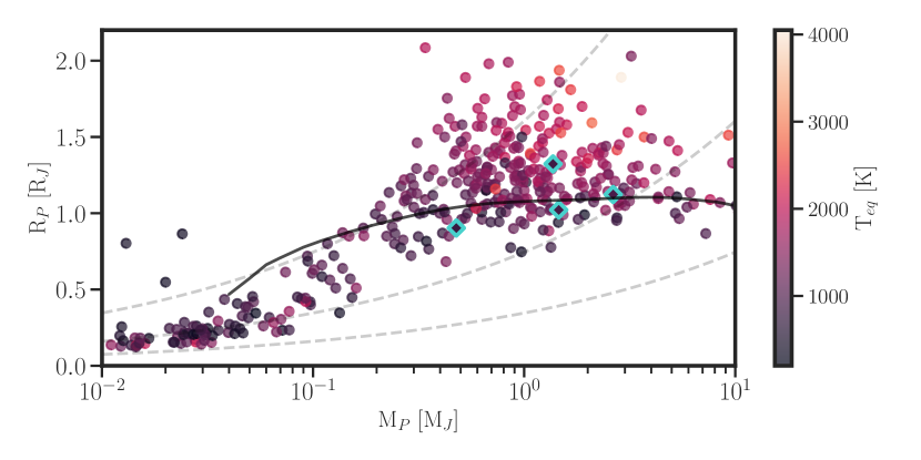
Figure 17: Mass–Radius diagram for the population of exoplanets with measured mass and radii. The points corresponding the discoveries presented in this work are indicated with diamonds. The color represents the equilibrium temperature of the planet. The dashed gray lines correspond to isodensity curves for 0.3, 3 and 30 g cm^-3 , respectively. The solid line corresponds to the predicted radius using the models of Fortney et al. (2007) for a planet with a 10 $M_{\oplus}$ central core.

We plot in Figure 18 the masses versus effective temperature for all planets that have both quantities measured in addition to their radii. We can see that three of the planets presented in this work have the higher masses known for transiting planets hosted by stars with $T_{\rm eff}\lesssim 4000$ K, with HATS-76b having a mass of $2.629\pm 0.089$, HATS-74Ab a mass of $1.46\pm 0.14$ and HATS-77b a mass of $1.374_{-0.074}^{+0.100}$. If we include radial velocity planets these masses are not particularly remarkable, and confirm the fact that despite their lower average protoplanetary disk masses these systems can assemble very massive giant planets. This result is in accord with formation models that find that, while the occurrence rate of giant planets is expected to decrease for M dwarfs, the maximum planetary mass is not (e.g., Burn et al., 2021).

The TESS mission, with its all-sky, high photometric precision survey, is allowing us to further the frontiers of exoplanet discoveries. While focused to a large degree on discovering small planets around nearby stars, the combination of its coverage with larger aperture facilities for photometric and spectroscopic follow-up, is allowing to efficiently target the rare class of giant planets around late K and later dwarfs with effective temperatures $\lesssim 4000$ K. In particular, the arrival of ESPRESSO to the VLT allows an efficiency in this quest heretofore unavailable in the southern hemisphere. We are undertaking a systematic search for these systems. With an increased sample of known giants around M dwarfs we expect to provide stronger constraints on the occurrence rates for these systems. Such occurance rates have remained to date too uncertain to effectively constrain models despite their unique potential. The clear prediction of core-accretion theory is that the efficiency of formation should decrease dramatically for stars with masses $M\lesssim 0.7M_{\odot}$. A higher efficiency of formation, above what models based on core-accretion predict, could be traced to the inadequacy some basic assumptions. For example, a basic tenet is that disk mass is proportional to stellar mass. While this is observationally well established, the dispersion at a given mass is significant and there are instances of young M stars with massive disks where gravitational instabilities may be a viable formation pathway for giant planets (e.g., the young M0 star Elias 2-27, see Paneque-Carreño et al., 2021, and references therein). A well determined occurrence rate for giant planets around M dwarfs will be invaluable in providing stringent tests for the current favoured models of planetary formation and evolution.

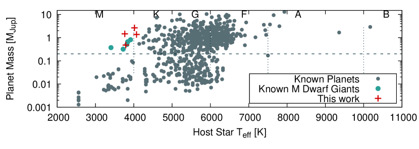
Figure 18: Mass versus effective temperature $T_{\rm eff}$ for confirmed transiting exoplanets. The dotted vertical lines indicate the $T_{\rm eff}$ values that roughly separate the spectral types as indicated on top, while the horizontal line at $M=0.2M_{\odot}$ indicates the adopted boundary between giant and smaller planets. Different symbols are used to plot known giants around M dwarfs and the discoveries presented in this work as indicated in the legend. Data were downloaded from the NASA Exoplanet Archive on May 13 2021.

Table 4: Astrometric, Spectroscopic and Photometric parameters for HATS-74A, HATS-75, HATS-76 and HATS-77

	HATS-74A	HATS-75	HATS-76	HATS-77
Parameter	Value	Value	Value	Value	Source
Astrometric properties and cross-identifications
2MASS-ID	11240360-1933257	04034783-2524320	04412154-3219128	09591770-2723339
TIC-ID	219189765	44737596	170849515	11561667
TOI-ID	737.01	552.01	555.01	730.01
GAIA DR2-ID	3545653561942122368	5082914338199586560	4877426575724467456	5466556141521710592
R.A. (J2000)	$11^{\mathrm{h}}24^{\mathrm{m}}03.5929{\mathrm{s}}$	$04^{\mathrm{h}}03^{\mathrm{m}}47.8440{\mathrm{s}}$	$04^{\mathrm{h}}41^{\mathrm{m}}21.5520{\mathrm{s}}$	$09^{\mathrm{h}}59^{\mathrm{m}}17.6640{\mathrm{s}}$	GAIA DR2
Dec. (J2000)	$-19{\arcdeg}33{\arcmin}25.6653{\arcsec}$	$-25{\arcdeg}24{\arcmin}32.1170{\arcsec}$	$-32{\arcdeg}19{\arcmin}13.5029{\arcsec}$	$-27{\arcdeg}23{\arcmin}34.1427{\arcsec}$	GAIA DR2
$\mu_{\rm R.A.}$ ($\rm mas\,yr^{-1}$)	$-38.86\pm 0.12$	$12.872\pm 0.038$	$-5.429\pm 0.057$	$-24.64\pm 0.10$	GAIA DR2
$\mu_{\rm Dec.}$ ($\rm mas\,yr^{-1}$)	$39.679\pm 0.077$	$-1.753\pm 0.048$	$-38.609\pm 0.090$	$-8.286\pm 0.098$	GAIA DR2
parallax (mas)	$3.425\pm 0.042$	$5.100\pm 0.029$	$2.564\pm 0.038$	$2.265\pm 0.056$	GAIA DR2
Spectroscopic properties
$T_{\rm eff\star}$ (K)	$3775\pm 54$	$3812\pm 79$	$3990\pm 120$	$4082\pm 69$	ARCoIRIS
$\rm[Fe/H]$	$0.294\pm 0.088$	$0.28\pm 0.12$	$0.29\pm 0.13$	$-0.12\pm 0.10$	ARCoIRIS
$\gamma_{\rm RV}$ ($\rm m\,s^{-1}$)	$15850\pm 12$	$39997.7\pm 5.4$	$8597\pm 11$	$-7758\pm 43$	ESPRESSO
Photometric properties
$P_{\rm rot}$ (d)	$4.745422\pm 0.000040$	$35.0435\pm 0.0017$	$15.16063\pm 0.00048$	$\cdots$	HATSouth
$G$ (mag)	$15.9706\pm 0.0029$	$14.90330\pm 0.00040$	$15.79420\pm 0.00060$	$15.7364\pm 0.0011$	GAIA DR2
$BP$ (mag)	$\cdots$	$16.0189\pm 0.0026$	$16.6962\pm 0.0057$	$16.5518\pm 0.0054$	GAIA DR2
$RP$ (mag)	$\cdots$	$13.8535\pm 0.0013$	$14.8610\pm 0.0020$	$14.8547\pm 0.0038$	GAIA DR2
$B$ (mag)	$\cdots$	$17.120\pm 0.019$	$\cdots$	$17.716\pm 0.010$	APASS
$V$ (mag)	$\cdots$	$15.759\pm 0.036$	$\cdots$	$16.354\pm 0.010$	APASS
$g$ (mag)	$\cdots$	$16.503\pm 0.070$	$\cdots$	$17.10\pm 0.25$	APASS
$r$ (mag)	$\cdots$	$15.156\pm 0.090$	$\cdots$	$15.746\pm 0.060$	APASS
$i$ (mag)	$\cdots$	$14.230\pm 0.070$	$\cdots$	$15.212\pm 0.010$	APASS
$J$ (mag)	$13.341\pm 0.023$	$12.481\pm 0.023$	$13.690\pm 0.029$	$13.779\pm 0.029$	2MASS
$H$ (mag)	$12.687\pm 0.029$	$11.756\pm 0.026$	$12.984\pm 0.024$	$13.047\pm 0.029$	2MASS
$K_{s}$ (mag)	$12.452\pm 0.031$	$11.584\pm 0.021$	$12.812\pm 0.033$	$12.934\pm 0.032$	2MASS
$W1$ (mag)	$12.342\pm 0.023$	$11.486\pm 0.024$	$12.758\pm 0.024$	$12.847\pm 0.024$	WISE
$W2$ (mag)	$12.326\pm 0.023$	$11.502\pm 0.022$	$12.784\pm 0.026$	$12.870\pm 0.027$	WISE
$W3$ (mag)	$\cdots$	$11.61\pm 0.19$	$\cdots$	$\cdots$	WISE

Table 5: ESPRESSO relative radial velocities and Bisector Spans for HATS-74A, HATS-75, HATS-76 and HATS-77.

System	BJD	RV	$\sigma_{\rm RV}$	BS	$\sigma_{\rm BS}$	Phase
	(2,450,000$+$)	($\rm m\,s^{-1}$)	($\rm m\,s^{-1}$)	($\rm m\,s^{-1}$)	($\rm m\,s^{-1}$)
HATS-74	$8843.81635$	$254.27$	$14.40$	$10.4$	$27.4$	$0.870$
HATS-74	$8844.82333$	$-116.73$	$18.60$	$5.3$	$37.0$	$0.451$
HATS-74	$8846.84777$	$242.27$	$13.40$	$15.5$	$25.4$	$0.620$
HATS-74	$8847.83295$	$-318.73$	$12.70$	$22.8$	$24.7$	$0.189$
HATS-74	$8848.83946$	$340.27$	$13.10$	$28.8$	$24.6$	$0.770$
HATS-75	$8756.72534$	$-93.43$	$10.80$	$-20.4$	$21.6$	$0.237$
HATS-75	$8759.70279$	$-90.43$	$9.40$	$36.1$	$18.8$	$0.304$
HATS-75	$8760.72353$	$91.57$	$12.80$	$17.9$	$25.6$	$0.670$
HATS-75	$8761.73812$	$-18.43$	$8.60$	$55.3$	$17.1$	$0.034$
HATS-75	$8762.77554$	$-49.43$	$8.20$	$45.8$	$16.4$	$0.406$
HATS-76	$8756.74359$	$-265.56$	$24.90$	$75.2$	$49.8$	$0.086$
HATS-76	$8759.72348$	$361.44$	$19.70$	$67.1$	$39.4$	$0.620$
HATS-76	$8762.81602$	$-565.56$	$16.10$	$62.7$	$32.3$	$0.213$
HATS-76	$8779.83962$	$101.44$	$19.20$	$34.9$	$38.3$	$0.981$
HATS-77	$8818.79874$	$-96.07$	$27.00$	$49.8$	$54.0$	$0.042$
HATS-77	$8820.78227$	$227.93$	$12.90$	$64.1$	$25.8$	$0.685$
HATS-77	$8836.81364$	$177.93$	$17.20$	$91.2$	$34.4$	$0.877$
HATS-77	$8843.73764$	$-143.07$	$17.50$	$108.3$	$35.1$	$0.119$
HATS-77	$8844.74086$	$-114.07$	$13.10$	$107.2$	$26.1$	$0.444$

Table 6: Adopted derived stellar parameters for HATS-74A, HATS-75, HATS-76 and HATS-77.

	HATS-74A	HATS-75	HATS-76	HATS-77
Parameter	Value	Value	Value	Value
$M_{\star}$ ($M_{\sun}$)	$0.6010\pm 0.0080$	$0.6017_{-0.0055}^{+0.0074}$	$0.662_{-0.021}^{+0.016}$	$0.655\pm 0.014$
$R_{\star}$ ($R_{\sun}$)	$0.5758\pm 0.0055$	$0.5848\pm 0.0026$	$0.6259\pm 0.0079$	$0.6428\pm 0.0066$
$\log{g_{\star}}$ (cgs)	$4.696\pm 0.011$	$4.6831\pm 0.0069$	$4.665\pm 0.016$	$4.638\pm 0.014$
$\rho_{\star}$ ($\rm g\,cm^{-3}$)	$4.43_{-0.14}^{+0.18}$	$4.239_{-0.065}^{+0.091}$	$3.80\pm 0.17$	$3.48_{-0.12}^{+0.17}$
$L_{\star}$ ($L_{\sun}$)	$0.0608\pm 0.0015$	$0.06359\pm 0.00069$	$0.0916\pm 0.0029$	$0.1019\pm 0.0028$
$T_{\rm eff\star}$ (K)	$3776.9\pm 9.5$	$3790.4\pm 5.7$	$4016\pm 17$	$4071\pm 13$
$\rm[Fe/H]$	$0.514_{-0.021}^{+0.033}$	$0.522_{-0.028}^{+0.051}$	$0.322_{-0.049}^{+0.065}$	$0.253\pm 0.039$
Age (Gyr)	$11.0\pm 5.1$	$14.9_{-4.3}^{+3.3}$	$4.6_{-4.0}^{+8.7}$	$12.1\pm 5.0$
$A_{V}$ (mag)	$0.1960_{-0.0150}^{+0.0100}$	$0.0560\pm 0.0095$	$0.062\pm 0.012$	$0.111_{-0.019}^{+0.013}$
Distance (pc)	$286.6\pm 3.0$0	$195.3\pm 1.0$	$389.9\pm 5.6$	$413.9\pm 5.9$
MB ($M_{\sun}$)	$0.2284\pm 0.0078$	$<0.38$	$<0.24$	$<0.53$

Note. — The listed parameters are those determined through the joint differential evolution Markov Chain analysis described in Section 3.1. For all four systems the RV observations are consistent with a circular orbit, and we assume a fixed circular orbit in generating the parameters listed here. Systematic errors in the bolometric correction tables or stellar evolution models are not included, and may dominate the error budget for some of these parameters.

Table 7: Adopted orbital and planetary parameters for HATS-74Ab, HATS-75b, HATS-76b and HATS-77b

	HATS-74Ab	HATS-75b	HATS-76b	HATS-77b
Parameter	Value	Value	Value	Value
Light curve parameters
$P$ (days)	$1.73185606\pm 0.00000055$	$2.7886556\pm 0.0000011$	$1.9416423\pm 0.0000014$	$3.0876262\pm 0.0000016$
$T_{c}$ (${\rm BJD\_{}TDB}$)	$2458392.02654\pm 0.00024$	$2458611.05487\pm 0.00027$	$2458424.55556\pm 0.00053$	$2459136.69378\pm 0.00020$
$T_{14}$ (days)	$0.06889\pm 0.00064$	$0.07969\pm 0.00065$	$0.0774\pm 0.0011$	$0.09282\pm 0.00070$
$T_{12}=T_{34}$ (days)	$0.01256\pm 0.00049$	$0.01256\pm 0.00036$	$0.01254\pm 0.00067$	$0.01610\pm 0.00061$
$a/R_{\star}$	$8.90\pm 0.10$	$12.037_{-0.062}^{+0.086}$	$9.12\pm 0.14$	$12.06_{-0.14}^{+0.19}$
$\zeta/R_{\star}$	$35.31_{-0.42}^{+0.56}$0	$29.71\pm 0.38$0	$30.76\pm 0.67$0	$26.02\pm 0.28$0
$R_{p}/R_{\star}$	$0.1844\pm 0.0030$	$0.1555\pm 0.0021$	$0.1772\pm 0.0045$	$0.1865\pm 0.0024$
$b^{2}$	$0.165_{-0.033}^{+0.029}$	$0.165_{-0.029}^{+0.024}$	$0.079_{-0.048}^{+0.051}$	$0.107_{-0.033}^{+0.028}$
$b\equiv a\cos i/R_{\star}$	$0.406_{-0.043}^{+0.034}$	$0.406_{-0.038}^{+0.029}$	$0.281_{-0.105}^{+0.080}$	$0.328_{-0.054}^{+0.041}$
$i$ (deg)	$87.39\pm 0.29$0	$88.07\pm 0.15$0	$88.24\pm 0.59$0	$88.44\pm 0.27$0
Dilution factors
HATSouth 1	$0.954\pm 0.046$	$0.756\pm 0.061$	$0.892\pm 0.056$	$0.906\pm 0.054$
HATSouth 2	$\cdots$	$0.956\pm 0.030$	$\cdots$	$\cdots$
TESS 1	$0.963\pm 0.033$	$0.937\pm 0.032$	$0.966\pm 0.033$	$0.9927\pm 0.0095$
TESS 2	$\cdots$	$0.949\pm 0.028$	$\cdots$	$\cdots$
Limb-darkening coefficients
$c_{1},g$	$0.39\pm 0.17$	$0.36\pm 0.13$	$0.47\pm 0.14$	$0.47\pm 0.12$
$c_{2},g$	$0.29\pm 0.20$	$0.34\pm 0.17$	$0.34\pm 0.15$	$0.38\pm 0.14$
$c_{1},r$	$0.40\pm 0.15$	$0.29\pm 0.12$	$0.34\pm 0.16$	$0.365_{-0.087}^{+0.117}$
$c_{2},r$	$0.23\pm 0.18$	$0.21\pm 0.17$	$0.31\pm 0.17$	$0.34\pm 0.15$
$c_{1},R$	$0.30\pm 0.14$	$\cdots$	$\cdots$	$\cdots$
$c_{2},R$	$0.29\pm 0.17$	$\cdots$	$\cdots$	$\cdots$
$c_{1},i$	$0.45\pm 0.14$	$\cdots$	$\cdots$	$0.34\pm 0.10$
$c_{2},i$	$0.27\pm 0.18$	$\cdots$	$\cdots$	$0.21_{-0.14}^{+0.18}$
$c_{1},zs$	$0.32\pm 0.12$	$0.170_{-0.090}^{+0.120}$	$\cdots$	$\cdots$
$c_{2},zs$	$0.17\pm 0.16$	$0.10\pm 0.16$	$\cdots$	$\cdots$
$c_{1},T$	$0.19_{-0.10}^{+0.14}$	$0.28\pm 0.12$	$0.34\pm 0.14$	$0.55\pm 0.15$
$c_{2},T$	$0.17\pm 0.17$	$0.34\pm 0.16$	$0.36\pm 0.17$	$0.35\pm 0.15$
RV parameters
$K$ ($\rm m\,s^{-1}$)	$346\pm 34$00	$99.2\pm 7.9$00	$562\pm 15$00	$253\pm 63$00
$e$	$<0.044$	$<0.064$	$<0.062$	$<0.045$
RV jitter ESPRESSO ($\rm m\,s^{-1}$)	$<32.1$	$<2.8$	$<19.0$	$<87.3$
Planetary parameters
$M_{p}$ ($M_{\rm J}$)	$1.46\pm 0.14$	$0.491\pm 0.039$	$2.629\pm 0.089$	$1.374_{-0.074}^{+0.100}$
$R_{p}$ ($R_{\rm J}$)	$1.032\pm 0.021$	$0.884\pm 0.013$	$1.079\pm 0.031$	$1.165\pm 0.021$
$C(M_{p},R_{p})$	$-0.01$	$-0.11$	$0.01$	$-0.01$
$\rho_{p}$ ($\rm g\,cm^{-3}$)	$1.64\pm 0.19$	$0.878\pm 0.084$	$2.58\pm 0.23$	$1.077_{-0.081}^{+0.112}$
$\log g_{p}$ (cgs)	$3.529\pm 0.063$	$3.192\pm 0.038$	$3.747\pm 0.029$	$3.398_{-0.028}^{+0.038}$
$a$ (AU)	$0.02384\pm 0.00011$	$0.032742_{-0.000099}^{+0.000134}$	$0.02658_{-0.00029}^{+0.00021}$	$0.03607\pm 0.00025$
$T_{\rm eq}$ (K)	$895.1\pm 5.7$	$772.3\pm 2.3$	$939.8\pm 6.7$	$828.3\pm 5.9$
$\Theta$	$0.112\pm 0.011$	$0.0602\pm 0.0049$	$0.1947\pm 0.0075$	$0.129\pm 0.032$
$\log_{10}\langle F\rangle$ (cgs)	$8.163\pm 0.011$	$7.9066\pm 0.0051$	$8.247\pm 0.012$	$8.028\pm 0.012$

Note. — For all systems we adopt a model in which the orbit is assumed to be circular. See the discussion in Section 3.1.

References

- Abbott et al. (2016) Abbott, T. M. C., Walker, A. R., Points, S. D., et al. 2016, in Proc. SPIE, Vol. 9906, Ground-based and Airborne Telescopes VI, 99064D, doi: 10.1117/12.2232723
- Astropy Collaboration et al. (2013) Astropy Collaboration, Robitaille, T. P., Tollerud, E. J., et al. 2013, A&A, 558, A33, doi: 10.1051/0004-6361/201322068
- Astropy Collaboration et al. (2018) Astropy Collaboration, Price-Whelan, A. M., Sipőcz, B. M., et al. 2018, AJ, 156, 123, doi: 10.3847/1538-3881/aabc4f
- Bakos et al. (2010) Bakos, G. Á., Torres, G., Pál, A., et al. 2010, ApJ, 710, 1724, doi: 10.1088/0004-637X/710/2/1724
- Bakos et al. (2013) Bakos, G. Á., Csubry, Z., Penev, K., et al. 2013, PASP, 125, 154, doi: 10.1086/669529
- Bakos et al. (2018) Bakos, G. Á., Bayliss, D., Bento, J., et al. 2018, arXiv e-prints, arXiv:1812.09406. https://arxiv.org/abs/1812.09406
- Bakos et al. (2020) —. 2020, AJ, 159, 267, doi: 10.3847/1538-3881/ab8ad1
- Bayliss et al. (2013) Bayliss, D., Zhou, G., Penev, K., et al. 2013, AJ, 146, 113, doi: 10.1088/0004-6256/146/5/113
- Bertin & Arnouts (1996) Bertin, E., & Arnouts, S. 1996, A&AS, 117, 393, doi: 10.1051/aas:1996164
- Bovy et al. (2016) Bovy, J., Rix, H.-W., Green, G. M., Schlafly, E. F., & Finkbeiner, D. P. 2016, ApJ, 818, 130, doi: 10.3847/0004-637X/818/2/130
- Brahm et al. (2017a) Brahm, R., Jordán, A., & Espinoza, N. 2017a, Publications of the Astronomical Society of the Pacific, 129, 034002, doi: 10.1088/1538-3873/aa5455
- Brahm et al. (2017b) Brahm, R., Jordán, A., Hartman, J., & Bakos, G. 2017b, MNRAS, 467, 971, doi: 10.1093/mnras/stx144
- Brahm et al. (2015) Brahm, R., Jordán, A., Hartman, J. D., et al. 2015, AJ, 150, 33, doi: 10.1088/0004-6256/150/1/33
- Brasseur et al. (2019) Brasseur, C. E., Phillip, C., Fleming, S. W., Mullally, S. E., & White, R. L. 2019, Astrocut: Tools for creating cutouts of TESS images. http://ascl.net/1905.007
- Brown et al. (2013) Brown, T. M., Baliber, N., Bianco, F. B., et al. 2013, PASP, 125, 1031, doi: 10.1086/673168
- Buchhave et al. (2012) Buchhave, L. A., Latham, D. W., Johansen, A., et al. 2012, Nature, 486, 375, doi: 10.1038/nature11121
- Burn et al. (2021) Burn, R., Schlecker, M., Mordasini, C., et al. 2021, arXiv e-prints, arXiv:2105.04596. https://arxiv.org/abs/2105.04596
- Cardelli et al. (1989) Cardelli, J. A., Clayton, G. C., & Mathis, J. S. 1989, ApJ, 345, 245, doi: 10.1086/167900
- Choi et al. (2016) Choi, J., Dotter, A., Conroy, C., et al. 2016, ApJ, 823, 102, doi: 10.3847/0004-637X/823/2/102
- Ciardi et al. (2015) Ciardi, D. R., Beichman, C. A., Horch, E. P., & Howell, S. B. 2015, ApJ, 805, 16, doi: 10.1088/0004-637X/805/1/16
- Clanton & Gaudi (2014) Clanton, C., & Gaudi, B. S. 2014, ApJ, 791, 91, doi: 10.1088/0004-637X/791/2/91
- Claret (2018) Claret, A. 2018, A&A, 618, A20, doi: 10.1051/0004-6361/201833060
- Claret et al. (2012) Claret, A., Hauschildt, P. H., & Witte, S. 2012, A&A, 546, A14, doi: 10.1051/0004-6361/201219849
- Claret et al. (2013) —. 2013, A&A, 552, A16, doi: 10.1051/0004-6361/201220942
- Collins et al. (2018) Collins, K., Quinn, S. N., Latham, D. W., et al. 2018, in American Astronomical Society Meeting Abstracts, Vol. 231, American Astronomical Society Meeting Abstracts #231, 439.08
- Collins et al. (2017) Collins, K. A., Kielkopf, J. F., Stassun, K. G., & Hessman, F. V. 2017, AJ, 153, 77, doi: 10.3847/1538-3881/153/2/77
- Cushing et al. (2004a) Cushing, M. C., Vacca, W. D., & Rayner, J. T. 2004a, PASP, 116, 362, doi: 10.1086/382907
- Cushing et al. (2004b) —. 2004b, PASP, 116, 362, doi: 10.1086/382907
- Demory & Seager (2011) Demory, B.-O., & Seager, S. 2011, ApJS, 197, 12, doi: 10.1088/0067-0049/197/1/12
- Dopita et al. (2007) Dopita, M., Hart, J., McGregor, P., et al. 2007, Ap&SS, 310, 255, doi: 10.1007/s10509-007-9510-z
- Dotter (2016) Dotter, A. 2016, ApJS, 222, 8, doi: 10.3847/0067-0049/222/1/8
- Doyle et al. (2011) Doyle, L. R., Carter, J. A., Fabrycky, D. C., et al. 2011, Science, 333, 1602, doi: 10.1126/science.1210923
- Fischer & Valenti (2005) Fischer, D. A., & Valenti, J. 2005, ApJ, 622, 1102, doi: 10.1086/428383
- Fortney et al. (2007) Fortney, J. J., Marley, M. S., & Barnes, J. W. 2007, ApJ, 659, 1661, doi: 10.1086/512120
- Freudling et al. (2013) Freudling, W., Romaniello, M., Bramich, D. M., et al. 2013, A&A, 559, A96, doi: 10.1051/0004-6361/201322494
- Furlan et al. (2017) Furlan, E., Ciardi, D. R., Everett, M. E., et al. 2017, AJ, 153, 71, doi: 10.3847/1538-3881/153/2/71
- Gaia Collaboration et al. (2018) Gaia Collaboration, Brown, A. G. A., Vallenari, A., et al. 2018, A&A, 616, A1, doi: 10.1051/0004-6361/201833051
- Gaidos & Mann (2014) Gaidos, E., & Mann, A. W. 2014, ApJ, 791, 54, doi: 10.1088/0004-637X/791/1/54
- Gonzalez (1998) Gonzalez, G. 1998, A&A, 334, 221
- Hansen & Barman (2007) Hansen, B. M. S., & Barman, T. 2007, ApJ, 671, 861, doi: 10.1086/523038
- Hartman & Bakos (2016) Hartman, J. D., & Bakos, G. Á. 2016, Astronomy and Computing, 17, 1, doi: 10.1016/j.ascom.2016.05.006
- Hartman et al. (2019) Hartman, J. D., Bakos, G. Á., Bayliss, D., et al. 2019, AJ, 157, 55, doi: 10.3847/1538-3881/aaf8b6
- Howell et al. (2016) Howell, S. B., Everett, M. E., Horch, E. P., et al. 2016, ApJ, 829, L2, doi: 10.3847/2041-8205/829/1/L2
- Howell et al. (2011) Howell, S. B., Everett, M. E., Sherry, W., Horch, E., & Ciardi, D. R. 2011, AJ, 142, 19, doi: 10.1088/0004-6256/142/1/19
- Hsu et al. (2019) Hsu, D. C., Ford, E. B., Ragozzine, D., & Ashby, K. 2019, AJ, 158, 109, doi: 10.3847/1538-3881/ab31ab
- Ida & Lin (2005) Ida, S., & Lin, D. N. C. 2005, ApJ, 626, 1045, doi: 10.1086/429953
- Jenkins et al. (2010) Jenkins, J. M., Caldwell, D. A., Chandrasekaran, H., et al. 2010, ApJ, 713, L87, doi: 10.1088/2041-8205/713/2/L87
- Jenkins et al. (2016) Jenkins, J. M., Twicken, J. D., McCauliff, S., et al. 2016, in Proc. SPIE, Vol. 9913, Software and Cyberinfrastructure for Astronomy IV, 99133E, doi: 10.1117/12.2233418
- Jensen (2013) Jensen, E. 2013, Tapir: A web interface for transit/eclipse observability, Astrophysics Source Code Library. http://ascl.net/1306.007
- Johnson et al. (2010) Johnson, J. A., Aller, K. M., Howard, A. W., & Crepp, J. R. 2010, PASP, 122, 905, doi: 10.1086/655775
- Johnson et al. (2012) Johnson, J. A., Gazak, J. Z., Apps, K., et al. 2012, AJ, 143, 111, doi: 10.1088/0004-6256/143/5/111
- Jordán et al. (2014) Jordán, A., Brahm, R., Bakos, G. Á., et al. 2014, AJ, 148, 29, doi: 10.1088/0004-6256/148/2/29
- Kaufer & Pasquini (1998) Kaufer, A., & Pasquini, L. 1998, in Society of Photo-Optical Instrumentation Engineers (SPIE) Conference Series, Vol. 3355, Optical Astronomical Instrumentation, ed. S. D’Odorico, 844–854
- Kovács et al. (2005) Kovács, G., Bakos, G., & Noyes, R. W. 2005, MNRAS, 356, 557, doi: 10.1111/j.1365-2966.2004.08479.x
- Kovács et al. (2002) Kovács, G., Zucker, S., & Mazeh, T. 2002, A&A, 391, 369, doi: 10.1051/0004-6361:20020802
- Lang et al. (2010) Lang, D., Hogg, D. W., Mierle, K., Blanton, M., & Roweis, S. 2010, AJ, 139, 1782, doi: 10.1088/0004-6256/139/5/1782
- Laughlin et al. (2004) Laughlin, G., Bodenheimer, P., & Adams, F. C. 2004, ApJ, 612, L73, doi: 10.1086/424384
- Lenzen et al. (2003) Lenzen, R., Hartung, M., Brandner, W., et al. 2003, in Society of Photo-Optical Instrumentation Engineers (SPIE) Conference Series, Vol. 4841, Instrument Design and Performance for Optical/Infrared Ground-based Telescopes, ed. M. Iye & A. F. M. Moorwood, 944–952, doi: 10.1117/12.460044
- Lightkurve Collaboration et al. (2018) Lightkurve Collaboration, Cardoso, J. V. d. M., Hedges, C., et al. 2018, Lightkurve: Kepler and TESS time series analysis in Python. http://ascl.net/1812.013
- Mandel & Agol (2002) Mandel, K., & Agol, E. 2002, ApJ, 580, L171, doi: 10.1086/345520
- Marigo et al. (2017) Marigo, P., Girardi, L., Bressan, A., et al. 2017, ApJ, 835, 77, doi: 10.3847/1538-4357/835/1/77
- Montet et al. (2014) Montet, B. T., Crepp, J. R., Johnson, J. A., Howard, A. W., & Marcy, G. W. 2014, ApJ, 781, 28, doi: 10.1088/0004-637X/781/1/28
- Morales et al. (2019) Morales, J. C., Mustill, A. J., Ribas, I., et al. 2019, Science, 365, 1441, doi: 10.1126/science.aax3198
- Mortier et al. (2013) Mortier, A., Santos, N. C., Sousa, S., et al. 2013, A&A, 551, A112, doi: 10.1051/0004-6361/201220707
- Mulders (2018) Mulders, G. D. 2018, Planet Populations as a Function of Stellar Properties, ed. H. J. Deeg & J. A. Belmonte, 153, doi: 10.1007/978-3-319-55333-7_153
- Narita et al. (2019) Narita, N., Fukui, A., Kusakabe, N., et al. 2019, Journal of Astronomical Telescopes, Instruments, and Systems, 5, 015001, doi: 10.1117/1.JATIS.5.1.015001
- Narita et al. (2020) Narita, N., Fukui, A., Yamamuro, T., et al. 2020, in Society of Photo-Optical Instrumentation Engineers (SPIE) Conference Series, Vol. 11447, Society of Photo-Optical Instrumentation Engineers (SPIE) Conference Series, 114475K, doi: 10.1117/12.2559947
- Newton et al. (2014) Newton, E. R., Charbonneau, D., Irwin, J., et al. 2014, AJ, 147, 20, doi: 10.1088/0004-6256/147/1/20
- Newton et al. (2015) Newton, E. R., Charbonneau, D., Irwin, J., & Mann, A. W. 2015, ApJ, 800, 85, doi: 10.1088/0004-637X/800/2/85
- Obermeier et al. (2016) Obermeier, C., Koppenhoefer, J., Saglia, R. P., et al. 2016, A&A, 587, A49, doi: 10.1051/0004-6361/201527633
- Pál (2012) Pál, A. 2012, MNRAS, 421, 1825, doi: 10.1111/j.1365-2966.2011.19813.x
- Paneque-Carreño et al. (2021) Paneque-Carreño, T., Perez, L. M., Benisty, M., et al. 2021, arXiv e-prints, arXiv:2103.14048. https://arxiv.org/abs/2103.14048
- Paxton et al. (2011) Paxton, B., Bildsten, L., Dotter, A., et al. 2011, ApJS, 192, 3, doi: 10.1088/0067-0049/192/1/3
- Paxton et al. (2013) Paxton, B., Cantiello, M., Arras, P., et al. 2013, ApJS, 208, 4, doi: 10.1088/0067-0049/208/1/4
- Paxton et al. (2015) Paxton, B., Marchant, P., Schwab, J., et al. 2015, ApJS, 220, 15, doi: 10.1088/0067-0049/220/1/15
- Penev et al. (2013) Penev, K., Bakos, G. Á., Bayliss, D., et al. 2013, AJ, 145, 5, doi: 10.1088/0004-6256/145/1/5
- Pepe et al. (2021) Pepe, F., Cristiani, S., Rebolo, R., et al. 2021, A&A, 645, A96, doi: 10.1051/0004-6361/202038306
- Rousset et al. (2003) Rousset, G., Lacombe, F., Puget, P., et al. 2003, in Society of Photo-Optical Instrumentation Engineers (SPIE) Conference Series, Vol. 4839, Adaptive Optical System Technologies II, ed. P. L. Wizinowich & D. Bonaccini, 140–149, doi: 10.1117/12.459332
- Sabotta et al. (2021) Sabotta, S., Schlecker, M., Chaturvedi, P., et al. 2021, arXiv e-prints, arXiv:2107.03802. https://arxiv.org/abs/2107.03802
- Santos et al. (2004) Santos, N. C., Israelian, G., & Mayor, M. 2004, A&A, 415, 1153, doi: 10.1051/0004-6361:20034469
- Schlieder et al. (2021) Schlieder, J. E., Gonzales, E. J., Ciardi, D. R., et al. 2021, Frontiers in Astronomy and Space Sciences, 8, 63, doi: 10.3389/fspas.2021.628396
- Smith et al. (2012) Smith, J. C., Stumpe, M. C., Van Cleve, J. E., et al. 2012, PASP, 124, 1000, doi: 10.1086/667697
- Stassun et al. (2017) Stassun, K. G., Collins, K. A., & Gaudi, B. S. 2017, AJ, 153, 136, doi: 10.3847/1538-3881/aa5df3
- Stassun et al. (2019) Stassun, K. G., Oelkers, R. J., Paegert, M., et al. 2019, AJ, 158, 138, doi: 10.3847/1538-3881/ab3467
- Stumpe et al. (2014) Stumpe, M. C., Smith, J. C., Catanzarite, J. H., et al. 2014, PASP, 126, 100, doi: 10.1086/674989
- Subasavage et al. (2010) Subasavage, J. P., Bailyn, C. D., Smith, R. C., et al. 2010, in Society of Photo-Optical Instrumentation Engineers (SPIE) Conference Series, Vol. 7737, Observatory Operations: Strategies, Processes, and Systems III, ed. D. R. Silva, A. B. Peck, & B. T. Soifer, 77371C, doi: 10.1117/12.859145
- Vacca et al. (2003) Vacca, W. D., Cushing, M. C., & Rayner, J. T. 2003, PASP, 115, 389, doi: 10.1086/346193
- Vacca et al. (2004) —. 2004, PASP, 116, 352, doi: 10.1086/382906
- Wang et al. (2003) Wang, S.-i., Hildebrand, R. H., Hobbs, L. M., et al. 2003, in Society of Photo-Optical Instrumentation Engineers (SPIE) Conference Series, Vol. 4841, Instrument Design and Performance for Optical/Infrared Ground-based Telescopes, ed. M. Iye & A. F. M. Moorwood, 1145–1156, doi: 10.1117/12.461447
- Wizinowich et al. (2000) Wizinowich, P., Acton, D. S., Shelton, C., et al. 2000, PASP, 112, 315, doi: 10.1086/316543
- Zacharias et al. (2013) Zacharias, N., Finch, C. T., Girard, T. M., et al. 2013, AJ, 145, 44, doi: 10.1088/0004-6256/145/2/44
- Zechmeister & Kürster (2009) Zechmeister, M., & Kürster, M. 2009, A&A, 496, 577, doi: 10.1051/0004-6361:200811296
- Zhu & Dong (2021) Zhu, W., & Dong, S. 2021, arXiv e-prints, arXiv:2103.02127. https://arxiv.org/abs/2103.02127
- Ziegler et al. (2018) Ziegler, C., Law, N. M., Baranec, C., et al. 2018, ArXiv e-prints. https://arxiv.org/abs/1806.10142