TRNR: Task-Driven Image Rain and Noise Removal with a Few Images Based on Patch Analysis

Abstract

The recent prosperity of learning-based image rain and noise removal is mainly due to the well-designed neural network architectures and large labeled datasets. However, we find that current image rain and noise removal methods result in low utilization of images. To alleviate the reliance on large labeled datasets, we propose the task-driven image rain and noise removal (TRNR) based on the introduced patch analysis strategy. The patch analysis strategy provides image patches with various spatial and statistical properties for training and has been verified to increase the utilization of images. Further, the patch analysis strategy motivates us to consider learning image rain and noise removal task-driven instead of data-driven. Therefore we introduce the N-frequency-K-shot learning task for TRNR. Each N-frequency-K-shot learning task is based on a tiny dataset containing NK image patches sampled by the patch analysis strategy. TRNR enables neural networks to learn from abundant N-frequency-K-shot learning tasks other than from adequate data. To verify the effectiveness of TRNR, we build a light Multi-Scale Residual Network (MSResNet) with about 0.9M parameters to learn image rain removal and use a simple ResNet with about 1.2M parameters dubbed DNNet for blind gaussian noise removal with a few images (for example, 20.0% train-set of Rain100H). Experimental results demonstrate that TRNR enables MSResNet to learn better from fewer images. In addition, MSResNet and DNNet utilizing TRNR have obtained better performance than most recent deep learning methods trained data-driven on large labeled datasets. These experimental results have confirmed the effectiveness and superiority of the proposed TRNR. The codes of TRNR will be public soon.

I Introduction

Computer vision algorithms such as autonomous driving[1], semantic segmentation[2], and object tracking[3] require clean images as input, and thus tend to fail under bad weather conditions. Image rain and noise removal, which are delicated to restore clean images from degraded observations, serve as the indispensable pre-processing process for those computer vision algorithms. Specifically, image rain and noise removal focus on removing the rain streaks [4, 5, 6, 7, 8] and removing noise [9, 10, 11, 12] from degraded images respectively via solving a linear decomposition problem.

Recent research on image rain and noise removal can be categorized into the prior-based approaches and the data-driven approaches. The prior-based approaches solve the linear decomposition problem via imposing artificially designed priors [4, 13, 6, 14]. While the data-driven approaches, e.g., [7, 11, 10, 15] enable models to learn more robustly and more flexibly with the help of large labeled datasets, which usually results in robust models with better performance. However, these data-driven approaches for image rain removal [16, 17, 18, 19] and noise removal [11, 10, 12] can not be adapted to limited data occasions due to over-fitting and low generalization ability.

(a)

(b)

(c)

(d)

(e). Rainy

(f). ReHEN [5]

(g). Ours

(h). GT

Figure 1: Image rain removal examples. (a) & (e) represent the image contaminated by complex and accumulated rains streaks. (b) & (f) indicate the image rain removal results of Yang et al. [5] that use the full train-set (700 images) for training. (c) & (g) are results of MSResNet (ours) that are trained with only 280 images. (d) & (h) are the Ground Truth.

Though data-driven approaches have made splendid progress, they have not made full use of large labeled datasets by employing the random image sampling (RIS) strategy to provide data for training. RIS leads to low utilization of image patches and neglects the spatial and statistical differences between different kinds of image patches. In practice, we observe that the performances of image rain and noise removal networks vary when tested on image patches with various spatial and statistical properties. This observation motivates us to discriminatively sample image patches for training. Therefore, we propose a patch analysis strategy to first divide image patches into different clusters according to the spatial and statistical properties. Then we introduce the random cluster sampling (RCS) strategy to provide data for training by randomly choosing image patches from different clusters, which is verified to make better use of image patches.

To overcome the data limitation problem for learning image rain and noise removal, we propose a task-driven approach to substitute the current data-driven approach for training neural networks. By considering image patches discriminatively according to spatial and statistical properties, we introduce the N-frequency-K-shot learning task. The N-frequency-K-shot learning task aims to learn image rain and noise removal on a tiny dataset consisting of image patches from $N$ clusters and each cluster with $K$ examples. During the training process, the neural network can learn from numerous N-frequency-K-shot tasks instead of learning from plenty of data. Concretely, the neural network first adapts itself to a batch of N-frequency-K-shot learning tasks, then it summaries the knowledge obtained from each task to make a significant update. The training process of neural networks with the TRNR approach is similar to the Model Agnostic Meta-Learning (MAML) that focuses on fast adaptation to unknown tasks. To prove the effectiveness of the proposed TRNR approach, we design a light Multi-Scale Residual Network (MSResNet) with about 0.9M parameters for image rain removal. We use a simple ResNet with about 1.2M parameters from [20] that we denote as DNNet in this paper for blind gaussian noise removal. In practice, MSResNet using the TRNR strategy with 100 images from Rain100L[15] (50.0% of train-set), 250 images from Rain100H[15] (20.0% of train-set), 280 images from Rain800[21] (40% of train-set), and DNNet using 500 images from BSD500[22] and Waterloo [23] (9.7% of train-set) have achieved impressive performances when compared to recent image rain removal [7, 15, 16, 24, 25, 5, 26, 27, 28] and gaussian noise removal [14, 11, 10, 29, 30, 31] models.

Fig. 1 presents two image rain removal examples from Rain800 [21] dataset. The model ReHEN[5] is trained using full train-set (700 images) while MSResNet is trained using 280 images. Fig. 1 indicates that MSResNet trained using fewer images can provide better results. To summarize, the contributions in this paper are summarized as below:

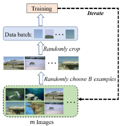
(a). Random Image Sampling (RIS)

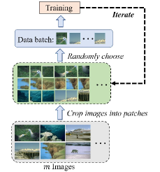
(b). Random Patch Sampling (RPS)

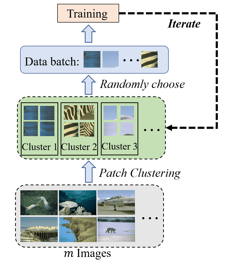
(c). Random Cluster Sampling (RCS)

Figure 2: Comparison of random sampling strategies. The green shaded box indicates the data used for sampling. (a) random image sampling, which is widely used by recent image rain removal models. (b) random patch sampling, which is utilized in DnCNN [11]. (c) random cluster sampling.

• We propose the patch analysis strategy to cluster image patches according to spatial and statistical properties. Patch analysis strategy utilizes RCS to sample image patches discriminatively for training. RCS can increase the utilization of image patches.

• We propose the task-driven approach dubbed TRNR for learning image rain and noise removal with a few images. TRNR trains neural networks with abundant N-frequency-K-shot learning tasks, and it boosts performance when data is limited.

• To prove the effectiveness and superiority of TRNR, we design MSResNet for image rain removal and use DNNet for blind gaussian noise removal. Experimental results on synthetic datasets have shown that MSResNet and DNNet perform better than most recent models while requiring fewer images for training. Experimental results on real-world rainy images demonstrate that the generalization ability of MSResNet is also guaranteed when using the proposed TRNR.

The organization of the remaining chapters is as follows. In §II, we review recent image rain and noise removal works together with few-shot learning. And in §III, we first elaborate the patch analysis strategy theoretically, then we detail the proposed task-driven approach and the architecture of MSResNet. We next carry out ablation studies and experiments on image rain and noise removal in §IV for the verification of the proposed TRNR. The conclusion is demonstrated in §V.

II Background and Related Work

II-A Image Rain and Noise Removal

Given degraded image $\mathrm{y}$, image rain and noise removal focus on restoring clean background $\mathrm{x}$ via solving the ill-posed linear decomposition problem formulated as Eq. (1). For image rain removal, $\mathrm{n}$ represents the rain layer[7, 5, 28] and $\mathrm{n}$ represents random noise for image noise removal [14, 11, 12, 20] respectively.

$$\mathrm{y}=\mathrm{x}+\mathrm{n}$$ (1)

As both described by the linear decomposition equation, image rain and noise removal are studied similarly. The basic assumption for solving Eq. (1) is that the information required for processing a degraded region is from its neighbors. In the prior-based perspective, the local information can be extracted via collaborative filtering[14], dictionary-learning [32, 6, 13, 33], and probabilistic modeling [4, 34], etc. These prior-based methods solve the linear decomposition problem iteratively with high time complexity.

With the rise of Deep Learning (DL), image rain and noise removal are coped with deep Convolutional Neural Networks (CNNs). CNNs can exploit rich information from image patches via skillfully stacking convolutional layers. The successes of CNNs on image rain and noise removal mainly stem from (1) fine-grained models [35, 12, 36, 15, 16, 5, 37, 8], (2) large labeled datasets [11, 7, 15, 24, 16, 5], and (3) specific learning algorithms [9, 12]. For instance, Wang et al. [28] propose a cross-scale multi-scale module to fuse features at different scales. Zhang et al. [24] build a large labeled dataset which provides 12,000 images for image rain removal. Liu et al. [12] embed traditional wavelet transformation into CNN for learning image noise removal with multi-scale wavelet CNN.

Generally, fine-grained models require large labeled datasets for training. The ingredients for building fine-grained models are residual connections [35, 16], recurrent units [15, 16, 5], attention mechanism [17], etc. [15, 24] have further introduced rain density label. Albeit successful and powerful, designing CNN and building large labeled datasets bring large human labor costs. In addition, the previous RIS strategy leads to insufficient utilization of large labeled datasets and ignores the differences between image patches. Therefore, we propose a patch analysis strategy in this paper to enable CNNs to learn discriminatively from image patches. Then we introduce a task-driven approach named TRNR for image rain and noise removal. Consequently, CNNs can learn image rain and noise removal from plentiful N-frequency-K-shot learning tasks rather than from large labeled datasets.

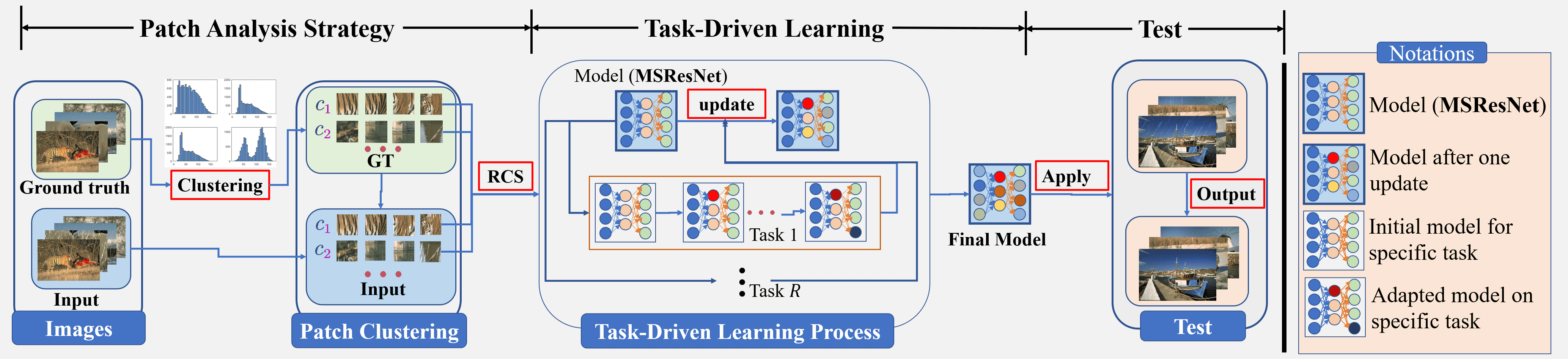
Figure 3: Overview of the proposed TRNR (image rain removal as an example). We first use the patch analysis strategy to crop images into patches and cluster all image patches. Then RCS is used for sampling N-frequency-K-shot tasks for training. At test time, we use the final model for testing.

II-B Meta-Learning

Meta-Learning, interpreted as learning to learn, aims to exploit meta-knowledge via learning on a set of tasks [38]. The learned meta-knowledge can help a neural network adapt fast to unknown tasks. Meta-Learning algorithms learn meta-knowledge via accumulating experience from multiple learning episodes. Specifically, the meta-learning algorithm first learns professional knowledge on a set of tasks with specific objectives and datasets (base-learning). Then, it integrates the learned professional knowledge to update meta-knowledge (meta-learning). Finn et al. [39] propose MAML to learn a good initialization of neural network parameters. MAML has been shown to work well for human pose estimation [40] and visual navigation [41]. In general, the proposed TRNR and MAML both learn from plenty of tasks. However, MAML aims to learn meta-knowledge for fast adaptation, but the proposed TRNR is devoted to exploiting rich information from a few images.

II-C Few-Shot Learning

Few-Shot Learning (FSL) focuses on learning a model with a few examples. With the help of prior knowledge, FSL can rapidly generalize to new tasks that contain only a few samples with supervision information [42]. FSL has made splendid progress on character generation, image classification, visual navigation, etc. The classical FSL problem is the N-way-K-shot classification, where the training data contains $NK$ examples from $N$ classes and each class with $K$ examples [42]. MAML has shown great potential in the N-way-K-shot classification. However, to the best of our knowledge, FSL for pixel-level image processing has rarely been explored, which is helpful when data is scarce. To deal with FSL for image rain and noise removal, we propose the task-driven approach TRNR.

III Task-Driven Image Rain and Noise Removal

In this section, we first detail the proposed patch analysis strategy in §III-A. In §III-B, we introduce the N-frequency-K-shot learning task based on the patch analysis strategy. Then we demonstrate the proposed task-driven approach for image rain and noise removal. In §III-C, we present the architecture of the MSResNet.

III-A Patch Analysis Strategy

Most recent DL based image rain removal models [7, 18, 15, 5, 16] and noise removal models [9, 11, 12, 31, 10] are trained with image patches utilizing RIS. Suppose a dataset $D=\{(x_{i},y_{i})\}_{i=1}^{m}$ contains $m$ examples, where $(x_{i},y_{i})$ indicates the $i$-th clean and degraded image pair following Eq. (1) respectively. Typically, we need to sample a data batch composed of $B$ clean and degraded image patch pairs at each training step, where $B$ means the batch size.

Take sampling $B$ clean image patches as an example, the most widely used RIS as shown in Fig. 2(a), provides $B$ image patches via cropping an image patch from each randomly sampled $B$ images. Analytically, RIS leads to low utilization of image patches. Generally, let $p^{unuse}_{k}$ denotes the probability that an image patch has not been sampled through $k$ iterations, $T_{e}$ denotes the total iterations of an epoch, and $P$ represents the number of patches that can be cropped out of an image. We can calculate $p^{unuse}_{k}$ analytically for RIS in Eq. (III-A).

(RIS): $$p^{unuse}_{k}=(1-\frac{B}{mP})^{k},$$

$$\text{s.t. }\ k\leq T_{e}=\frac{m}{B},\ B\leq m$$ (2)

Note that $p^{unuse}_{k}$ have minimum near to $\mathrm{e}^{-1/P}$for RIS when $k=T_{e}$ and $P$ is always a large number for RIS. For example, an image of size $321\times 481$ can crop $P=\lfloor\frac{321-64}{16}+1\rfloor\lfloor\frac{481-64}{16}+1\rfloor=459$ image patches of size $64\times 64$ with stride as $16$. One way to increase utilization of image patches is random patch sampling (RPS) as shown in Fig. 2(b). RPS first crops $m$ images into $mP$ image patches for sampling, which is still feasible when $m\leq B$ while RIS fails. $p^{unuse}_{k}$ for RPS is formulated in Eq. (3). Both RIS and RPS regard image patches equally, which may result in data redundancy. For example, as shown in Fig. 2, the sky scene in data batches sampled from RIS and RPS is redundant. In practice, the sky scene patches contain limited information and thus will contribute to a plain update of parameters.

$$\text{(RPS): }\ p^{unuse}_{k}=1-k\frac{B}{mP},\text{ s.t. }k\leq T_{e}=\frac{mP}{B}$$ (3)

Further, we propose the patch analysis strategy to improve the data utilization as shown in Fig. 3. For convenience, we only consider clean images dataset $D^{(c)}=\{x_{i}\}_{i=1}^{m}$ since clean image and degraded image are pairwise. First, we crop all $m$ images in $D^{(c)}$ to build clean image patches dataset $D^{(p,c)}=\{p_{i}\}_{i=1}^{N^{(p)}}$ where $N^{(p)}=mP$ means the total number of patches and $p_{i}$ denotes the $i$-th patch. Second, we cluster all $N^{(p)}$ image patches into $C$ clusters such that $D^{(p,c)}=\cup_{j=1}^{C}D^{(p,c)}_{j}$, and $D^{(p,c)}_{j}=\{p^{(j)}_{i}\}_{i=1}^{N^{(p)}_{j}}$, where $p^{(j)}_{i}$ denotes the $i$-th patch in $j$-th cluster and $N^{(p)}_{j}$ means the number of patches in cluster $j$.

To obtain a data batch composed of $B$ image patches, we first choose $B$ clusters among total $C$ clusters, then we randomly sample one image patch with replacement from each cluster to form a data batch. We call this sampling random cluster sampling (RCS) as shown in Fig. 2(c). Mathematically, if an image patch belongs to cluster $j$, then $p^{unuse}_{k}$ can be analytically derived as Eq. (III-A). Note that when $N^{(p)}_{j}\leq N^{(p)}/C$, RCS increases the utilization compared to RIS. Furthermore, RCS does not have data redundancy problem and treats image patches discriminatively.

(RCS): $$p^{unuse}_{k}=\left(1-\frac{B}{CN^{(p)}_{j}}\right)^{k}$$

$$\text{s.t. }\ k\leq T_{e}=\frac{N^{(p)}}{B}$$ (4)

As for the clustering, we employ the euclidean distance and the Kullback-Leibler (KL) divergence [43] as the distance metrics for image patches. We summarize the clustering method in Algorithm 1.

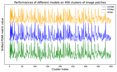
Figure 4: Performances of DnCNN [11], FFDNet [10], NLNet [31] on 400 clusters of image patches. Different methods tend to simultaneously behave well or bad on the specific cluster of image patches. We shift the curves for the comparison of tendency.

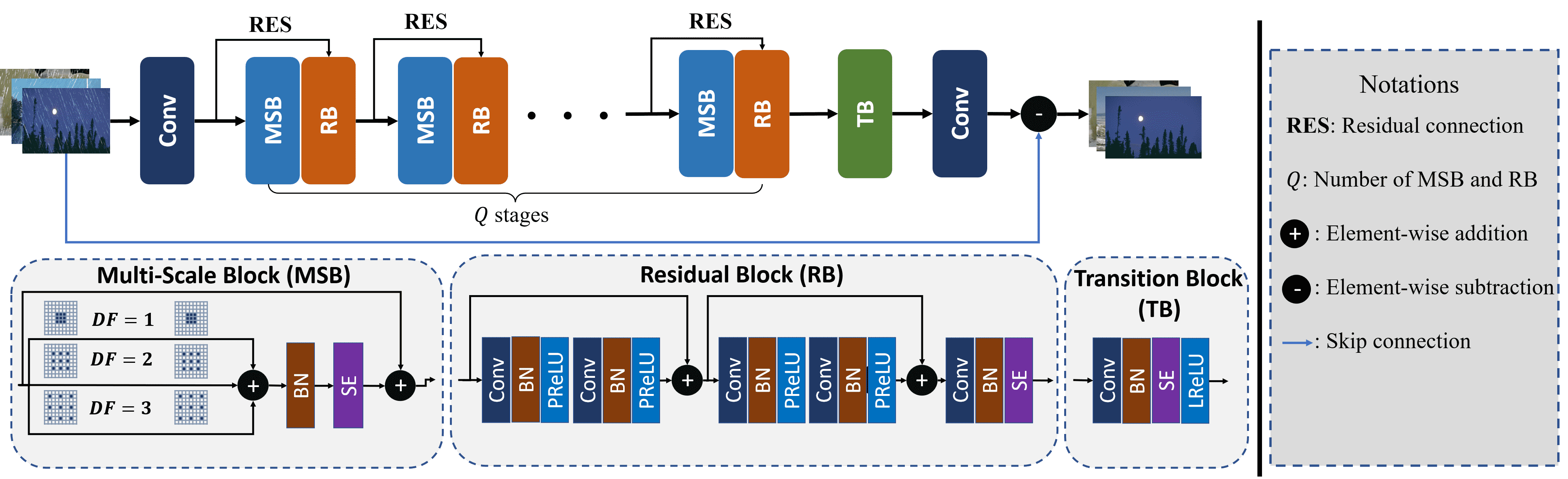
Figure 5: The whole structure of Multi-Scale Residual Neural Network (MSResNet) for image de-raining and denoise. ”RES” means adding a residual connection.

Algorithm 1 Patch Clustering Algorithm

0:  Clean dataset $D^{(c)}=\{x_{i}\}_{i=1}^{m}$, number of clusters $C$, threshold $T$, momentum $\rho=0.05$.

0:  Patch clusters $D^{(p,c)}=\cup_{j=1}^{C}D_{j}^{(p,c)}$

1:  Initialize $D_{j}^{(p,c)}=\{\}$ for $j=1$ to $C$. Set cluster centers $r_{j}=0$ for $j=1$ to $C$.

2:  Generate clean patches $D^{(p,c)}=\{p_{i}\}_{i=1}^{N^{(p)}}$ from input dataset $D^{(c)}$.

3:  Randomly choose one patch $p_{1}$ from $D^{(p,c)}$. Set $D_{1}^{(p,c)}=\{p_{1}\}$, and cluster center $r_{1}$=$p_{1}$.

4:  Initialize current cluster index $Idx=1$.

5:  for $k=2$ to $N^{(p)}$ do

6:     Compute distance $d$ between $p_{k}$ and all cluster centers $r_{j}$ for $j=1$ to $Idx$.

7:     Find the smallest $d$ and corresponded $j$.

8:     if $d<T$ or $Idx>=C$ then

9:        /* add patch to cluster $Idx$         */

10:        $D_{j}^{(p,c)}=D_{j}^{(p,c)}\bigcup\{p_{k}\}$

11:        if $Idx<C$ then

12:           /* update cluster center         */

13:           $r_{Idx}=(1-\rho)\times r_{Idx}+\rho\times p_{k}$

14:        end if

15:     else

16:        /* new cluster added           */

17:        $Idx=Idx+1$

18:        $D_{Idx}^{(p,c)}=\{p_{k}\}$

19:        $r_{Idx}=p_{k}$

20:     end if

21:  end for

III-B Task-Driven Approach Based on Patch Analysis

The goal of the patch analysis strategy is not only to improve the utilization of image patches but also to generate N-frequency-K-shot learning task distribution $p(\mathcal{T})$. From the clustering results, we empirically observe that deep neural networks, such as DnCNN [11], FFDNet [10], and NLNet [31] tend to simultaneously behave bad or well on image patches from the same cluster as shown in Fig. 4. This indicates that performing image rain and noise removal on image patches from the same cluster can be regarded as a sub-task.

N-frequency-K-shot Learning Task. As we have clustered image patches into $C$ clusters, we can define the N-frequency-K-shot learning task $\tau\sim p(\mathcal{T})$. Formally, let $f_{\theta}$ represent the model parameterized with $\theta$. Then the target of N-frequency-K-shot learning task $\tau_{j}$ sampled from $p(\mathcal{T})$ is to find the optimal parameters $\theta_{j}^{*}$ with $\theta$ as an initialization as shown in Eq. (5).

$$\theta_{j}^{*}=\arg\min_{\theta}\mathcal{L}_{\tau_{j}}(f_{\theta},\mathcal{D}_{\tau_{j}}^{(train)})$$ (5)

where $\mathcal{D}_{\tau_{j}}^{(train)}$ is the train-set for task $\tau_{j}$, which contains $NK$ image patches sampled from $N$ image patch clusters and each cluster with $K$ image patches. $\mathcal{L}_{\tau_{j}}$ denotes the loss function for $\tau_{j}$. Similarly, we denote the validation set for $\tau_{j}$ as $\mathcal{D}^{(val)}_{\tau_{j}}$. The task-driven approach aims to enable the neural network to learn from abundant tasks while each task contains different kinds of image patches for training.

Task-Driven Approach. The data-driven methods update parameters by taking a small step along the opposite direction of gradients computed on a batch of data. Analogically, the proposed task-driven approach TRNR updates the parameters $\theta$ by taking a small step along the opposite direction of gradients computed on a batch of tasks. In practice, TRNR first samples a batch of $R$ N-frequency-K-shot learning tasks $\{\tau_{j}\}_{j=1}^{R}$. Then it adapts the model parameters $\theta$ to each task via gradient descent as formulated in Eq. (6), where $\theta_{j}$ means the adapted parameters for task $\tau_{j}$ and $\alpha$ is the step size hyperparameter. Note that the model $f_{\theta_{j}}$ parameterized with $\theta_{j}$ now can perform well on task $\tau_{j}$, which indicates that $f_{\theta_{j}}$ can process $N$ kinds of image patches from N-frequency-K-shot learning task $\tau_{j}$.

$$\theta_{j}=\theta-\alpha\nabla_{\theta}\mathcal{L}_{\tau_{j}}(f_{\theta},\mathcal{D}^{(train)}_{\tau_{j}}),\ j=1,\cdots,R$$ (6)

To take full advantage of image patches that belong to sampled $R$ tasks and make the model learn from these $R$ tasks, we need to make a significant update for model parameters $\theta$. Suppose that the updated model parameters are denoted as $\tilde{\theta}$, TRNR updates parameters $\theta$ by taking the inequality formulated as Eq. (7) as a goal, which means that the performance of the model parameterized with updated parameters $\tilde{\theta}$ on the validation set of all $R$ tasks need to be no worse than the model parameterized with initial parameters $\theta$.

$$\sum_{j=1}^{R}\mathcal{L}_{\tau_{j}}(f_{\tilde{\theta}},\mathcal{D}^{(val)}_{\tau_{j}})\leq\sum_{j=1}^{R}\mathcal{L}_{\tau_{j}}(f_{\theta},\mathcal{D}^{(val)}_{\tau_{j}})$$ (7)

We make an approximation of $\tilde{\theta}$ as formulated in Eq. (8), which summaries the gradients of $\theta_{j}\ (j=1,\cdots,R)$ on the validation set of $\tau_{j}\ (j=1,\cdots,R)$. Eq. (6) and Eq. (8) can be explained under the MAML framework, where Eq. (6) represents the base-learning process and Eq. (8) represents the meta-learning process respectively.

$$\tilde{\theta}=\theta-\beta\nabla_{\theta}\frac{1}{R}\sum_{j=1}^{R}\mathcal{L}_{\tau_{j}}(f_{\theta_{j}},\mathcal{D}^{(val)}_{\tau_{j}})$$ (8)

Fig. 3 illustrates the proposed TRNR for learning image rain removal with a few samples. By changing MSResNet to DNNet in Fig. 3, we obtain the task-driven approach for image noise removal. In short, we present the details of task-driven learning in Algorithm 2.

Algorithm 2 Proposed TRNR Learning Algorithm

0:  Deep neural network $f_{\theta}$, step size hyperparameters $\alpha,\beta$, task distribution $p(\mathcal{T})$, Clustered image patches dataset $D^{(p,c)}=\cup_{j=1}^{C}D_{j}^{(p,c)}$

0:  well-trained model $f_{\theta*}$

1:  while not converge do

2:     Sample $R$ N-frequency-K-shot learning tasks $\{\tau_{j}\}$ from $p(\mathcal{T})$

3:     for $j=1$ to $R$ do

4:        /*  Learning on $R$ tasks            */

5:        Sample $\mathcal{D}^{(train)}_{\tau_{j}}$ from $D^{(p,c)}$ for task $\tau_{j}$ using RCS strategy

6:        Adapt $\theta$ to task $\tau_{j}$ as an initialization

7:        Compute adapted parameters $\theta_{j}$ for $\tau_{j}$ in Eq. (6)

8:        Sample $\mathcal{D}^{(val)}_{\tau_{j}}$ from $D^{(p,c)}$ for task $\tau_{j}$

9:     end for

10:     /*  Summarize gradients from $R$ tasks     */

11:     Compute updated model parameters $\tilde{\theta}$ in Eq. (8) using all $\theta_{j}$ and $\mathcal{D}^{(val)}_{\tau_{j}}$

12:     Initialize the model with parameters $\theta=\tilde{\theta}$

13:  end while

14:  Let $\theta^{*}=\tilde{\theta}$

15:  return  well-trained model $f_{\theta^{*}}$

III-C Multi-Scale Residual Neural Network (MSResNet)

To better balance network complexity against the computational overhead, we introduce three basic blocks in the proposed Multi-Scale Residual Neural Network (MSResNet), which include Multi-Scale Block (MSB), Residual Block (RB), and Transition Block (TB). Multi-scale design and residual connection have been proved to be effective in image rain removal [15, 16, 5, 19] and noise removal [11, 12, 35, 36]. The details of MSResNet are illustrated in Fig. 5.

Multi-Scale Block (MSB) MSB is used for enlarging the receptive field and aggregating feature maps of different scales. As shown in Fig. 5, at each stage, MSB takes the output from the previous RB as input except the first MSB. Inspired by the multi-scale design in [44], we use parallel atrous convolution [45] layers with different dilation rates to extract multi-scale information in MSB, and apply squeeze-and-excitation (SE) block [46] to exploit cross-channel information.

Residual Block (RB) Residual connection [47] has become indispensable in modern deep CNNs. In this paper, we construct a simple residual block (RB). As shown in Fig. 5, each RB takes the output of the previous MSB as input. There are two residual connections in each RB to aggregate features from different Conv-BN-PReLU modules. At the end of each RB, a SE block is used to further explore the cross-channel information.

To obtain better rain layers for image rain removal, we apply a skip connection from each MSB to its adjacent MSB as illustrated in Fig. 5 with “RES”.

Transition Block (TB) After processing input features via $Q$ MSBs and RBs ($Q$ stages), we utilize a transition block named TB to integrate features for inferring the rain layer and noise layer. The configuration of TB is illustrated in Fig. 5. Specifically, TB takes the summation of the outputs at the last two RBs as input to extract rich features. Similar to the design of MSB and DB, we place a SE block at the bottom of TB.

Loss function Since MSE loss tends to blur restored images, we combine L1 loss and SSIM loss following [48] for all N-frequency-K-shot learning tasks $\tau\sim p(\mathcal{T})$. Mathematically, let $(p,\tilde{p})$ denote the clean patch and corresponding degraded patch pair in $\mathcal{D}^{(train)}_{\tau_{j}}$. And $\hat{p}=f_{\theta_{j}}(\tilde{p})$ indicates the restored patch. Then the loss function $\mathcal{L}_{\tau_{j}}$ for task $\tau_{j}$ is formulated below in Eq. (9),

$$\mathcal{L}_{\tau_{j}}(f_{\theta},\mathcal{D}^{(train)}_{\tau_{j}}) =\mathbb{E}_{(p,\tilde{p})}\left[||p-\hat{p}||_{1}\right]$$

$$+\lambda\mathbb{E}_{(p,\tilde{p})}\left[1-\text{SSIM}(p,\hat{p})\right]$$

$$\text{s.t. }\tau_{j}\sim p(\mathcal{T})$$ (9)

where $\lambda$ is a hyperparameter.

TABLE I: Detail Settings of Datasets for Data-Driven and Task-Driven Rain and Noise Removal. #Train-patch and #Train-cluster Indicate Total Training Patches and Clusters for TRNR. The Test-set for WaterlooBSD is 222 Images from Set12, McMaster, Kodak, BSD68, and Urban100. w/o Indicates that RIS Samples from Images, Therefore Train-patch and Train-clustser are Not Necessary.

Type (Strategy)	Data-Driven (RIS)				Task-Driven (TRNR)
Datasets	Rain100L [15]	Rain100H [15]	Rain800 [21]	WaterlooBSD	Rain100L-S	Rain100H-S	Rain800-S	WaterlooBSD-S
Train-set	200	1254	700	5176	100	250	280	500
#Train-patch	w/o	w/o	w/o	w/o	22003	57329	73276	162764
#Train-cluster	w/o	w/o	w/o	w/o	4003	4829	5090	5968
Test-set	100	100	100	222	100	100	100	222

IV Experiments

In this section, we conduct extensive experiments to demonstrate the effectiveness of the proposed TRNR approach. For data-driven image rain removal, we train MSResNet using RIS separately on synthetic datasets Rain100L [15], Rain100H [15], Rain800 [21], and denote it as MSResNet-RIS. Correspondingly, we train DNNet using RIS on WaterlooBSD which contains 5176 images collected from BSD [22] and Waterloo [23] for image blind gaussian noise removal and note it as DNNet-RIS. As for TRNR, we construct corresponding small datasets for the above synthetic datasets, denoted as Rain100L-S, Rain100H-S, Rain800-S, and WaterlooBSD-S. Similarly, the neural networks are referred to as MSResNet-TRNR and DNNet-TRNR. Details of datasets are presented in Table I. We evaluate MSResNet-RIS and MSResNet-TRNR on synthetic datasets Rain100L [15], Rain100H [15], Rain800 [21] and real-world images collected from [15, 49, 17]. Datasets BSD68 [22], Kodak, McMaster [50], and Urban100 [51] are utilized for color image blind gaussian noise removal evaluation. Relatively, Set12, BSD68 [22], and Urban100 [51] are used for grayscale image blind gaussian noise comparison. Image rain and noise removal are evaluated in terms of Peak Signal-to-Noise Ratio (PSNR) [52], and Structural Similarity (SSIM) [53] metrics. And we compute PSNR and SSIM metrics over RGB channels for color images.

IV-A Training Details

Basic Training Settings. We set $Q=4$ for MSResNet, which means there are $4$ MSBs and RBs. Moreover, the filters of all convolution layers in MSResNet have the size of $3\times 3$ and 48 channels. And the negative slopes for all LeakyReLU activations are $0.2$. We first train MSResNet-RIS for image rain removal and DNNet-RIS for image blind gaussian noise removal. Then we train MSResNet-TRNR and DNNet-TRNR utilizing the proposed TRNR with a few images. The noise level in the training process of DNNet-RIS and DNNet-TRNR is uniformly in the range [0, 55]. The structure of DNNet follows the setting in [20]. Both MSResNet and DNNet are implemented using PyTorch [54] and trained with Adam optimizer on NVIDIA GeForce RTX 2060 SUPER GPU.

Task-Driven Image Rain Removal Settings. We train MSResNet-TRNR that possesses about 0.92M parameters using TRNR for image rain removal. In the task-learning process, $N$ and $K$ are $12$ and $1$ respectively for N-frequency-K-shot learning tasks. The batch size $R$ of N-frequency-K-shot learning tasks is set as $5$ in Eq. (8). The parameter $\lambda$ that leverages the loss items is $5$. Step size hyperparameters $\alpha$ and $\beta$ are both set to $0.001$.

Task-Driven Image Noise Removal Settings. We train DNNet-TRNR with about 1.2M parameters using TRNR for image blind gaussian noise removal. In the task-learning process, $N$ and $K$ are $70$ and $1$ for N-frequency-K-shot learning tasks. The batch size $R$ of N-frequency-K-shot learning tasks is set as $3$ in Eq. (8). We do not impose SSIM loss which complies with DnCNN [11] and FFDNet [10]. Step size hyperparameters $\alpha$ and $\beta$ are both set to $0.001$.

IV-B Ablation Study

In this subsection, we make a further study of the proposed MSResNet and TRNR strategy. Specifically, we primarily analyze the design of MSResNet to find the best combinations of different modules. Then we compare the widely used strategy RIS with RPS, RCS, and TRNR to show that the network trained using RIS suffers a heavy performance drop against using TRNR. Next, we determine the best configuration for task-driven learning, which includes the choices for $N$ in N-frequency-K-shot learning tasks and the batch size $R$ in Eq. (8). At last, we make a survey on RIS, RPS, RCS, and TRNR when dataset size is from 40 to 100 to prove the robustness of TRNR.

TABLE II: Average PSNR and SSIM Metrics on Test-Set of Rain100L of Different Designs. MS Means Multi-Scale Module and SE Indicates the SE Block.

Design	MS	SE	Q=3	Q=4	Q=5	PSNR/SSIM
Baseline	$\times$	$\times$	$\surd$	$\times$	$\times$	34.56/0.965
$N_{1}$	$\surd$	$\times$	$\surd$	$\times$	$\times$	34.72/0.967
$N_{2}$	$\times$	$\surd$	$\surd$	$\times$	$\times$	34.59/0.966
$N_{3}(Q=3)$	$\surd$	$\surd$	$\surd$	$\times$	$\times$	34.91/0.967
$N_{3}(Q=4)$	$\surd$	$\surd$	$\times$	$\surd$	$\times$	35.12/0.967
$N_{3}(Q=5)$	$\surd$	$\surd$	$\times$	$\times$	$\surd$	34.95/0.966

Analysis of the MSResNet Design. We begin by examining the importance of different modules in MSResNet. In particular, we regard MSResNet (Q=3) without multi-scale design in MSB, without all SE blocks as the Baseline. And we construct $3$ networks listed as follows for comparison:

• $N_{1}$: Baseline with multi-scale design in each MSB.

• $N_{2}$: Baseline with SE blocks at the bottom of all MSB, RB, and TB.

• $N_{3}$: $N_{1}$ with SE blocks at the bottom of all MSB, RBs, and TB.

We use RIS to train all of the above networks on the entire Rain100L train-set and then evaluate them on the Rain100L test-set. Table II displays the results in terms of PSNR/SSIM measurements. Adding multi-scale design or SE blocks can both enhance performance, as illustrated in Table II. Furthermore, multi-scale design and SE blocks have mutually beneficial impacts. We then conduct experiments on the number of MSB and RB in MSResNet, denoted as $Q$. From Table II, we find that $Q=4$ brings the best performance. Visual examples on the first row of Fig. 7 depict that MSResNet with $Q=3$ tends to under-derain and $Q=5$ tend to over-derain.

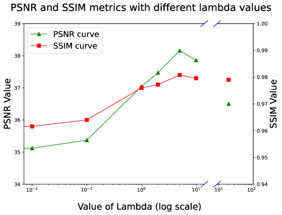
Figure 6: Test PSNR and SSIM Metrics when $\lambda$ in Eq. (9) varies from 0.01 to 10. The points on the right are obtained by using only SSIM loss for training, which indicates $\lambda$ is infinity in Eq. (9).

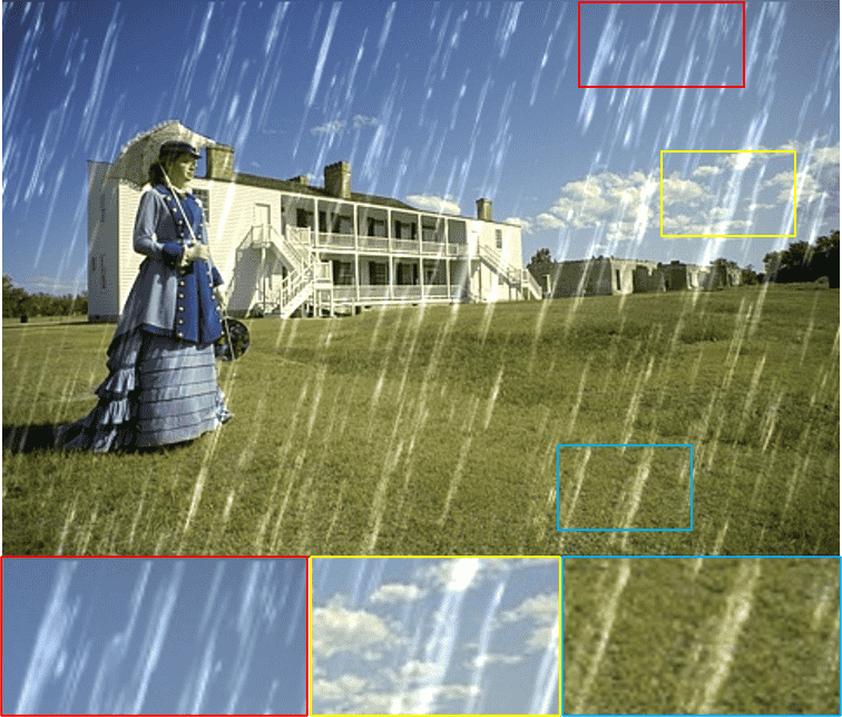
Rainy Image (22.86/0.767)

$Q=3$, $\lambda=0$ (32.10/0.960)

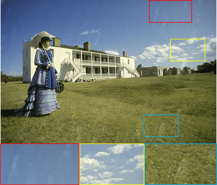
$Q=4$, $\lambda=0$ (32.93/0.963)

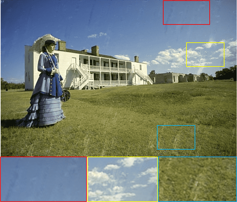
$Q=5$, $\lambda=0$ (32.30/0.960)

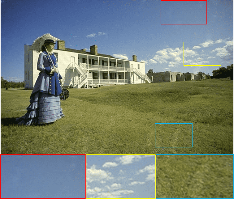
$Q=4$, $\lambda=1.0$ (34.79/0.977)

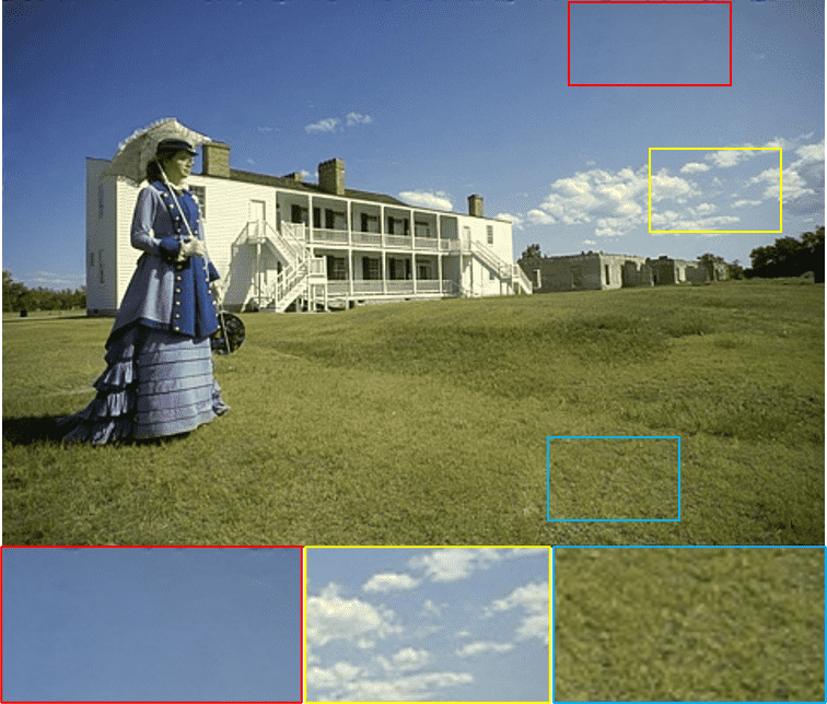
$Q=4$, $\lambda=5.0$ (35.81/0.980)

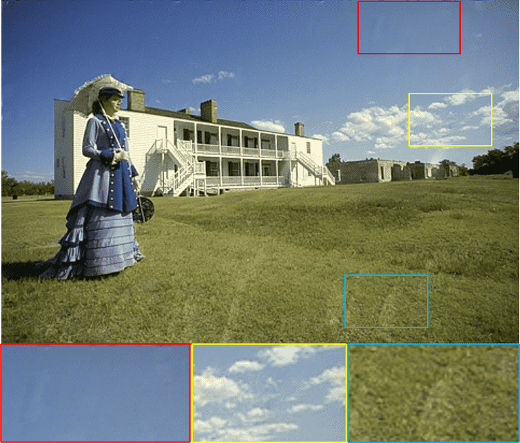
$Q=4$, $\lambda\to\infty$ (33.42/0.973)

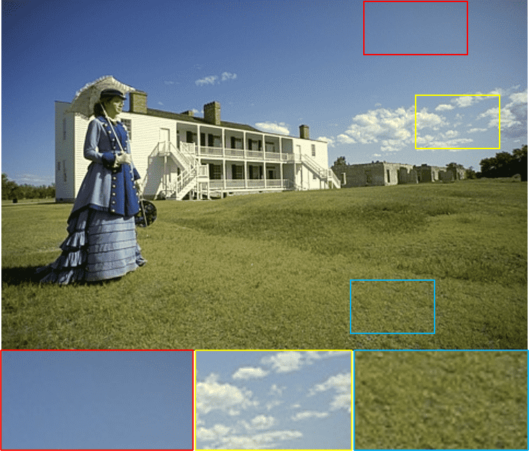
Ground Truth (Inf/1.0)

Figure 7: Image rain removal results of MSResNet with different $Q$ and trained using different $\lambda$ in loss function.

Ablation on Loss Function. Since SSIM loss has been proven to boost image rain removal performance [5, 17, 28, 19, 26], we make an ablation study on $\lambda$ which leverages the SSIM loss term in Eq. (9). Fig. 6 shows the testing PSNR and SSIM metrics on Rain100L when $\lambda$ varies. As can be seen from Fig. 7, the SSIM loss term leads to more reasonable image rain removal results. However, only employing SSIM loss term tend to under-derain.

Comparison of Learning Strategies. We compare the data-driven learning strategies using RIS, RPS, and RCS, as well as the task-driven learning strategy TRNR, after determining the best settings for MSResNet. We train MSResNet using RIS, RPS, RCS, and TRNR for 50,000 iterations on Rain100L-S as shown in Table I and use the test-set of Rain100L for evaluation. The evaluation results are presented in Table III. Quantitative results in Table III indicate that MSResNet using the RIS strategy offers the worst performance. MSResNet using TRNR has achieved 38.17/0.984 in terms of PSNR and SSIM metrics. TRNR has brought improvements on PSNR metric by 0.99dB, and SSIM metric by 0.4% against RIS strategy, which reveals the effectiveness of TRNR.

TABLE III: Quantitative Comparison of Data-Driven Learning Strategies and Task-Driven Learning Strategy. The Average PSNR and SSIM Metrics are Computed on the Test-Set of Rain100L.

Learning strategies	Different combinations
Data-Driven+RIS	$\surd$	$\times$	$\times$	$\times$
Data-Driven+RPS	$\times$	$\surd$	$\times$	$\times$
Data-Driven+RCS	$\times$	$\times$	$\surd$	$\times$
Task-Driven+TRNR	$\times$	$\times$	$\times$	$\surd$
PSNR	37.18	37.50	38.02	38.17
SSIM	0.980	0.982	0.983	0.984

TABLE IV: Average PSNR and SSIM Metrics on the Test-Set of Rain100L of Different $N$ and $R$ Combinations ($K$ is Set to 1).

($N$, $R$)	(32, 1)	(26, 2)	(18, 3)	(14, 4)	(12, 5)
PSNR	37.75	37.91	38.07	37.97	38.17
SSIM	0.982	0.983	0.984	0.983	0.984

Task-Driven Learning Settings. The proposed TRNR has obtained the best performance as shown in Table III. We then make a further investigation on the task-driven learning settings. In practice, $K$ is fixed to $1$ as some clusters only have 2 image patches (one for $\mathcal{D}^{(train)}_{\tau_{j}}$ and one for $\mathcal{D}^{(val)}_{\tau_{j}}$). Therefore, we investigate different combinations of $N$ in N-frequency-K-shot learning and batch size $R$ of sampled tasks number in Eq. (8). Intuitively, larger $N$ leads to greater memory requirements, and larger $R$ often results in better performance but longer training time as shown in Algorithm 2. Practically, we train MSResNet with $Q=4$ on 5 combinations of $N$ and $R$ and evaluate using test-set of Rain100L. The results in Table IV indicate that $N=12$ with $R=5$ provides the best performance.

Analysis on Dataset Size. Larger dataset for training often results in more robust models with better performances and better generalization ability. But how can we obtain a feasible model when the train-set only contains a few samples? In this paper, we propose to maximize the utilization of the dataset. Hence, we compare the TRNR with RIS, RPS, and RCS strategies when the train-set size varies from 40 images to 100 images. Note that RCS samples image patches discriminatively by increasing the utilization of image patches from the rare cluster (patch number is small than average patches number per cluster). As shown in Fig. 8(b), the proposed TRNR approach has the following advantages against RIS, RPS, and RCS strategies: (1) More stable training process due to task-driven learning. (2) Faster convergence. (3) Better training performance. Fig. 8 (a) provides the test PSNR metric on Rain100L when train-set size changes from 40 images to 100 images. When train-set size varies, the proposed TRNR has shown the greatest performance among all strategies. For example, when using 80 images for training, TRNR obtains 38.02dB in terms of PSNR metric, with 0.95dB improvement against RIS strategy, 0.61dB improvement against RPS strategy, and 0.22dB improvement over RCS strategy.

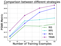
(a). Different train-set size

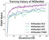
(b). Traning history of MSResNet

Figure 8: Comparison of RIS, RPS, and RCS with proposed TRNR when train-set size varies from 40 to 100 images. (a) denotes the test PSNR metric of different train-set sizes. (b) shows the training history of different strategies on PSNR metric when using 80 images for training.

Learn More From Less. Although TRNR has achieved the best performance against RIS, RPS, and RCS strategies, we still need to investigate the differences between models trained using TRNR on a few images and models trained using RIS strategy on full train-set. Therefore we compare the performances of MSResNet-RIS and MSResNet-TRNR on Rain100L, Rain100H, and Rain800. The quantitative results are presented in Table V. Note that MSResNet-TRNR has obtained higher PSNR/SSIM metrics against MSResNet-RIS. For instance, test PSNR/SSIM metrics for MSResNet-TRNR on Rain100H are 28.69/0.899, with 0.95dB/1.1% gain in terms of PSNR/SSIM against MSResNet-RIS. The quantitative results in Table V demonstrate that MSResNet-TRNR can learn more from less data, thus proving the effectiveness of the proposed TRNR.

TABLE V: Quantitative Evaluation Results on Rain100L, Rain100H, and Rain800 Datasets of MSResNet-TRNR and Other Recent Learning-Based Methods. The Best Results are Bolded, and The Second and Third Results are Highlighted in Red and Blue Colors, Respectively.

Methods	Rain100L		Rain100H		Rain800
	PSNR	SSIM	PSNR	SSIM	PSNR	SSIM
Rainy	25.52	0.825	12.13	0.349	21.15	0.651
JCAS (ICCV’17) [13]	28.40	0.881	13.65	0.459	22.19	0.766
DerainNet (TIP’17) [55]	27.36	0.855	13.94	0.403	23.14	0.771
DDN (CVPR’17) [7]	32.04	0.938	24.95	0.781	21.16	0.732
JORDER (CVPR’17) [15]	36.11	0.970	22.15	0.674	22.24	0.776
RESCAN (ECCV’18) [16]	36.64	0.975	26.45	0.846	24.09	0.841
DID-MDN (CVPR’18) [24]	25.70	0.858	17.39	0.612	21.89	0.795
DualCNN (CVPR’18) [25]	26.87	0.860	14.23	0.468	24.09	0.841
PReNet (CVPR’19) [48]	36.28	0.977	27.65	0.882	-	-
ReHEN (ACM’MM’19) [5]	37.41	0.980	27.97	0.864	26.96	0.854
DCSFN (ACM’MM’20) [28]	35.25	0.976	29.70	0.907	-	-
BRN (TIP’20) [26]	36.75	0.979	29.02	0.900	-	-
MPRNet (CVPR’21) [27]	35.01	0.960	28.54	0.872	28.75	0.876
MSResNet-TRNR (Ours)	38.17	0.984	28.69	0.899	28.62	0.892
MSResNet-RIS (Ours)	38.16	0.984	27.74	0.888	28.49	0.885

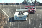
23.03/0.816

25.70/0.857

34.42/0.972

31.85/0.939

36.78/0.982

Inf/1.0

20.32/0.0.553
Rainy

21.98/0.769
DDN [7]

33.32/0.972
DCSFN [28]

27.35/0.922
MPRNet [27]

36.78/0.984
MSResNet-TRNR (Ours)

Inf/1.0
Ground Truth

Figure 9: Image rain removal results of DDN [7], DCSFN [28], MPReNet [27] and proposed method on Rain100L dataset. Values at the bottom of every image indicate the PSNR/SSIM metrics respectively.

20.77/0.596

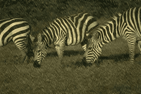
22.68/0.682

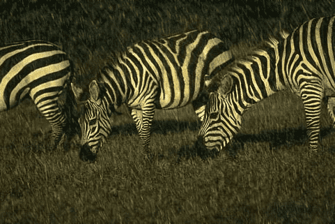
18.64/0.637

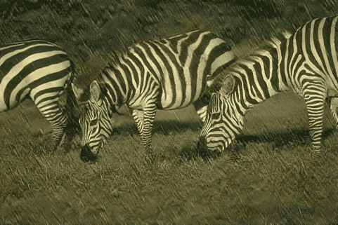
26.27/0.718

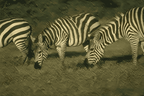
27.51/0.901

Inf/1.0

20.32/0.0.553
Rainy

18.39/0.784
ReHEN [5]

18.46/0.636
MPRNet [27]

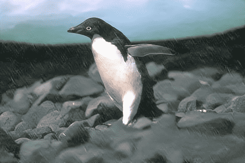
27.30/0.850
MSResNet-RIS (Ours)

27.22/0.798
MSResNet-TRNR (Ours)

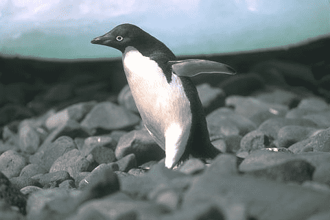
Inf/1.0
Ground Truth

Figure 10: Image rain removal visual examples of ReHEN [7], MPReNet [27] and proposed method on Rain800 dataset. Values at the bottom of every image indicate the PSNR/SSIM metrics respectively. ReHEN [5] and MPRNet [27] both fail to recover the background illuminance.

IV-C Comparisons on Synthetic Datasets

Image Rain Removal. We carry out experiments to verify the effectiveness of proposed TRNR approach. In practice, we train MSResNet-TRNR using TRNR separately on Rain100L-S, Rain100H-S and Rain800-S. The MSResNet-TRNR is compared with prior based method JCAS [13] and learning methods DerainNet [55], DDN [7], JORDER [15], RESCAN [16], DID-MDN [24], PReNet [48], ReHEN [5], DCSFN [28], JDNet [19], BRN [26], and MPRNet [27]. We use the official pre-trained MPRNet for evaluation due to too large number of parameters. These compared methods except JCAS [13] are all trained on large labeled datasets due to fine-grained models or large number of parameters. The quantitative results are provided in Table V. As can be seen from Table V, the MSResNet-TRNR has achieved better performance than prior based method JCAS [13], and learning based methods DDN [7], JORDER [15], RESCAN [16], PReNet [48], and ReHEN [5] over all compared datasets. Further, MSResNet-TRNR has obtained the first place on Rain100L dataset. Fig. 9 and Fig. 10 have shown 4 image rain removal examples of DDN [7], DCSFN [28], MPRNet [27] and MSResNet-TRNR. Although MSResNet-TRNR has not shown outstanding results on Rain100H and Rain800 datasets in Table V, MSResNet-TRNR has achieved better performance than ReHEN [5], DCSFN [28], BRN [26], and MPRNet [27] on real-world images as shown in Fig. 13.

TABLE VI: Average PSNR/SSIM Metrics for Color Image Blind Gaussian Noise Removal on McMaster, Kodak, BSD68 and Urban100 datasets. Noise Levels are 15, 25, 35, and 50. the Best Results are Bolded, and the Second and Third Results are Highlighted in Red and Blue Colors, Respectively.

Datasets	Noise Level	BM3D[14]	DnCNN[11]	NLNet[31]	FFDNet[10]	BUIFD[29]	PaCNet[30]	DNNet-RIS	DNNet-TRNR
McMaster	15	34.06/0.911	34.70/0.922	34.10/0.912	34.67/0.922	34.37/0.917	34.24/0.9162	34.98/0.927	34.92/0.926
	25	31.66/0.870	32.38/0.887	31.72/0.872	32.37/0.887	32.18/0.883	32.18/0.884	32.72/0.895	32.67/0.894
	35	29.92/0.829	30.83/0.857	-	30.83/0.855	30.69/0.853	-	31.22/0.867	31.18/0.866
	50	28.28/0.780	29.18/0.818	28.47/0.791	29.20/0.815	29.09/0.814	29.01/0.813	29.63/0.831	29.59/0.830
Kodak	15	34.28/0.915	34.62/0.922	34.53/0.920	34.64/0.922	34.64/0.921	34.69/0.922	34.91/0.926	34.87/0.925
	25	31.68/0.867	32.13/0.879	31.97/0.876	32.14/0.878	32.17/0.879	32.14/0.878	32.47/0.886	32.44/0.885
	35	29.90/0.821	30.56/0.842	-	30.57/0.841	30.61/0.842	-	30.94/0.852	30.90/0.851
	50	28.23/0.767	28.97/0.797	28.71/0.789	28.98/0.794	29.02/0.797	28.96/0.794	29.37/0.810	29.34/0.809
BSD68	15	33.52/0.922	33.84/0.929	33.79/0.928	33.89/0.929	33.93/0.929	33.95/0.930	33.89/0.930	33.85/0.929
	25	30.71/0.867	31.20/0.883	31.06/0.880	31.23/0.883	31.28/0.883	31.28/0.882	31.32/0.885	31.29/0.885
	35	28.89/0.816	29.58/0.842	-	29.59/0.841	29.65/0.843	-	29.73/0.847	29.70/0.846
	50	27.14/0.753	27.96/0.791	27.71/0.784	27.98/0.789	28.02/0.792	27.92/0.788	28.16/0.799	28.12/0.798
Urban100	15	33.95/0.941	33.94/0.943	33.88/0.942	33.84/0.942	33.71/0.939	33.87/0.941	33.79/0.944	34.15/0.946
	25	31.38/0.909	31.50/0.914	31.35/0.910	31.40/0.912	31.35/0.909	31.60/0.913	31.41/0.918	31.85/0.920
	35	29.27/0.873	29.87/0.886	-	29.79/0.885	29.76/0.881	-	29.91/0.894	30.31/0.896
	50	27.67/0.832	28.10/0.849	27.82/0.840	28.05/0.848	28.04/0.843	28.12/0.848	28.28/0.862	28.65/0.864

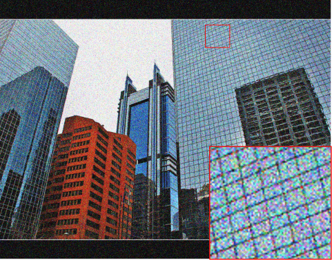
14.15/0.265

25.95/0.817

25.68/0.775

25.97/0.814

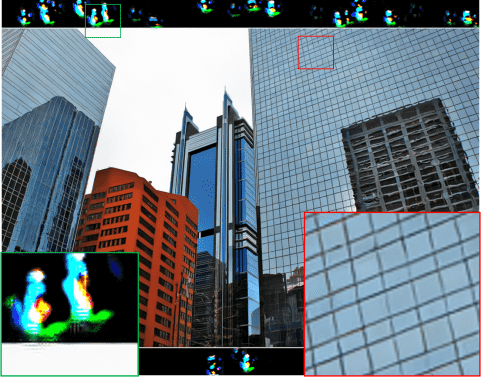
20.75/0.802

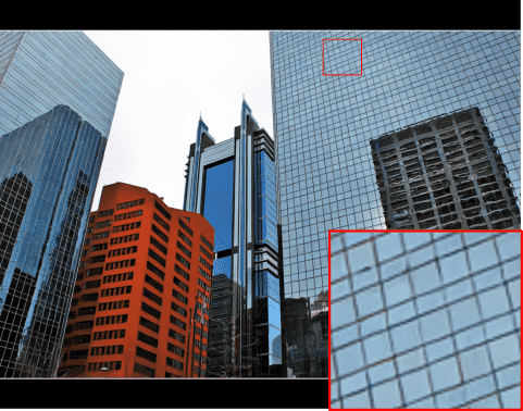
26.53/0.835

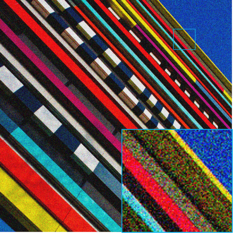
14.16/0.134
Noisy

31.97/0.876
FFDNet [10]

31.13/0.834
BUIFD [29]

31.60/0.814
PaCNet [30]

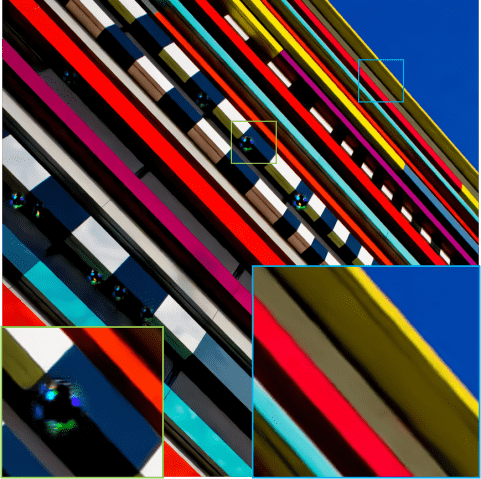
29.36/0.894
DNNet-RIS (Ours)

33.24/0.908
DNNet-TRNR (Ours)

Figure 11: Color image noise removal visual examples of FFDNet [10], BUIFD [29], PaCNet [30] and proposed DDNet-RIS, DDNet-TRNR on Urban100 dataset. Noise level is 50. Values at the bottom of every image indicate the PSNR/SSIM metrics respectively.

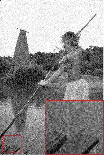
20.17/0.294

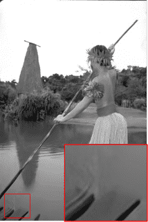
30.23/0.874

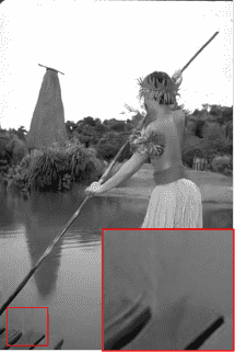
30.17/0.867

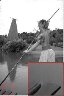
30.41/0.878

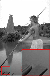
30.37/0.878

20.19/0.574
Noisy

26.38/0.871
FFDNet [10]

26.35/0.869
BUIFD [29]

26.51/0.876
DNNet-RIS (Ours)

26.48/0.875
DNNet-TRNR (Ours)

Figure 12: Grayscale image noise removal visual examples of FFDNet [10], BUIFD [29], and proposed DDNet-RIS, DDNet-TRNR on BSD68 dataset. Noise level is 25. Values at the bottom of every image indicate the PSNR/SSIM metrics respectively.

Color Image Blind Gaussian Noise Removal. To further investigate the proposed TRNR for learning image noise removal, we compare DNNet with recent prior based method BM3D [14], and deep learning based methods DnCNN [11], NLNet [31], FFDNet [10], BUIFD [29], and PaCNet [30] on color image blind gaussian noise removal with noise levels set to 15, 25, 35 and 50. In practice, we train DNNet-RIS on WaterlooBSD and DNNet-TRNR on WaterlooBSD-S which only contains about 0.16M image patches. The quantitative results are presented in Table VI. Since NLNet [31] and PaCNet [30] are not blind noise removal method, the PSNR/SSIM metrics for NLNet and PaCNet on noise level $35$ are vacant in Table VI. From Table VI, we can observe that DNNet-RIS has achieved the state-of-the-art performance. And DNNet-TRNR trained using WaterlooBSD-S (9.7% of WaterlooBSD) becomes comparable with DNNet-RIS. Fig. 11 provides 2 noise removal examples in Urban100 dataset when noise level set to 50. The compared methods in Fig. 11 are FFDNet [10], BUIFD [29], PaCNet [30], DNNet-RIS and DNNet-TRNR. As shown in Fig. 11, DNNet-RIS and DNNet-TRNR can better restore textures against FFDNet [10], BUIFD [29], and PaCNet [30]. Surprisingly, we find DNNet-TRNR performs better than DNNet-RIS on Urban100 datasets. For instance, DNNet-TRNR has provided 0.44dB gain in terms of PSNR on Urban100 when noise level equals 25. This bizarre observation can be interpreted in Fig. 11, where DNNet-RIS recovers image textures well but fail to process the black block region since black block region rarely emerges in images from WaterlooBSD. On the contrary, DNNet-TRNR can handle black block region well, thus demonstrating the potential of TRNR.

TABLE VII: Average PSNR/SSIM Metrics for Grayscale Image Blind Gaussian Noise Removal on Set12, BSD68, and Urban100. Noise Levels are 15, 25, 35, and 50. the Best Results are Bolded, and the Second and Third Results are Highlighted in Red and Blue Colors, Respectively.

Datasets	Noise Level	BM3D[14]	DnCNN[11]	NLNet[31]	FFDNet[10]	BUIFD[29]	DNNet-RIS	DNNet-TRNR
Set12	15	32.37/0.895	32.86/0.903	32.73/0.901	32.75/0.903	32.50/0.897	32.99/0.906	32.95/0.905
	25	29.97/0.850	30.48/0.863	30.31/0.857	30.43/0.864	30.19/0.856	30.67/0.869	30.64/0.868
	35	28.40/0.813	28.93/0.830	-	28.91/0.831	28.66/0.821	29.17/0.838	29.14/0.838
	50	26.50/0.757	27.28/0.787	27.02/0.779	27.30/0.790	27.02/0.776	27.57/0.799	27.53/0.798
BSD68	15	31.07/0.872	31.69/0.891	31.51/0.886	31.64/0.891	31.50/0.884	31.77/0.893	31.73/0.892
	25	28.57/0.801	29.22/0.828	28.99/0.817	29.19/0.829	29.07/0.821	29.32/0.833	29.29/0.833
	35	27.09/0.748	27.73/0.779	-	27.72/0.780	27.58/0.770	27.86/0.787	27.83/0.786
	50	25.44/0.675	26.27/0.721	26.02/0.709	26.29/0.724	26.12/0.711	26.41/0.733	26.38/0.731
Urban100	15	32.32/0.921	32.71/0.928	32.60/0.926	32.40/0.927	31.92/0.912	32.91/0.933	32.78/0.931
	25	29.69/0.877	30.13/0.889	29.93/0.884	29.90/0.888	29.47/0.870	30.43/0.898	30.33/0.896
	35	27.89/0.836	28.40/0.853	-	28.25/0.853	27.82/0.831	28.81/0.867	28.71/0.864
	50	25.65/0.766	26.54/0.801	26.17/0.791	26.50/0.805	26.06/0.779	27.07/0.824	26.97/0.821

Rainy

ReHEN [5]

DCSFN [28]

BRN [27]

MPRNet [27]

MSResNet-TRNR (ours)

Figure 13: Real-world image rain removal examples of ReHEN [5], DCSFN [28], BRN [26], MPRNet [27] and MSResNet-TRNR.

Grayscale Image Blind Gaussian Noise Removal. To prove the effectiveness of TRNR on grayscale image noise removal when there is no cross-channel information in input images, we compare DNNet with prior based method BM3D [14], deep learning based methods DnCNN [11], NLNet [31], FFDNet [10], and BUIFD [29]. We train DNNet-RIS on WaterlooBSD and DNNet-TRNR on WaterlooBSD-S. And then we use Set12, BSD68, and Urban100 for blind gaussian noise evaluation removal with noise levels set to 15, 25, 35, and 50. Table VII reports the grayscale image noise removal results. And DNNet-RIS has shown state-of-the-art performance overall datasets and noise levels. As for DNNet-TRNR trained using 9.7% of WaterlooBSD, it has outperformed recent extraordinary methods, e.g. DnCNN [11], FFDNet [10], and BUIFD [29]. It is worth noticing that DNNet-TRNR has also obtained competitive performance against DNNet-RIS, which has verified the effectiveness of TRNR. We also present 2 visual examples of grayscale noise removal in Fig. 12 to show the superiority of TRNR. The result on the first row of Fig. 12 demonstrate MSResNet-RIS and MSResNet-TRNR can remove noise from images better than FFDNet [10] and BUIFD [29]. While the result in the second row illustrates that MSResNet-RIS and MSResNet-TRNR can recover more details.

IV-D Comparisons on Real-World Dataset

Although the proposed MSResNet trained with the TRNR has shown great performance on synthetic datasets while requiring fewer images for training, the generalization ability of MSResNet on real-world images is unknown. Therefore, we compare DNNet-TRNR with recent image rain removal methods on real-world rainy images collected from [15, 17], and [49]. MSResNet-TRNR for real-world image rain removal is trained on Rain800-S. Fig. 13 provides 7 real-word image rain removal examples. As can be seen from Fig. 13, MSResNet-TRNR can better remove rain streaks and recover background compared with ReHEN [5], DCSFN [28], BRN [26], MPReNet [27]. Note that MSResNet-TRNR is trained on Rain800-S with only 280 images. Hence, the real-world image rain removal results prove that MSResNet-TRNR can generalize well on real-world occasions.

V Conclusion

Recent deep learning methods for image rain and noise removal require large labeled datasets for training. In order to alleviate the reliance on large labeled datasets, we have proposed the task-driven image rain and noise removal (TRNR) by introducing the patch analysis strategy. In TRNR, we first use the patch analysis strategy to improve the utilization of image patches, then we propose the N-frequency-K-shot learning tasks to enable the deep learning models to learn from abundant tasks. To verify the proposed TRNR, we have conducted ample experiments on image rain removal and blind gaussian noise removal. Experiments on both synthetic datasets and real-world datasets have proved the superiority and effectiveness of TRNR when training data is limited. It is noteworthy that there exists room for further study of TRNR. One direction is to employ TRNR in real scenarios where we can only collect a few examples. Another direction is building N-frequency-K-shot learning tasks by dynamically clustering image patches from data batches rather than pre-clustering all image patches. Because clustering $N^{(p)}$ image patches into $C$ clusters has $O(CN^{(p)})$ time complexity, which is not feasible when number of images $m$ is large.

References

- [1] G. Andreas, L. Philip, and U. Raquel, “Are we ready for autonomous driving? the kitti vision benchmark suite,” in Proceedings of the IEEE Conference on Computer Vision and Pattern Recognition, 2012, pp. 3354–3361.
- [2] M. Sachin, R. Mohammad, C. Anat, S. Linda, and H. Hannaneh, “Espnet: Efficient spatial pyramid of dilated convolutions for semantic segmentation,” in Proceedings of the European Conference on Computer Vision, 2018, pp. 552–568.
- [3] C. Dorin, R. Visvanathan, and M. Peter, “Kernel-based object tracking,” IEEE Transactions on Pattern Analysis and Machine Intelligence, vol. 25, no. 5, pp. 564–577, 2003.
- [4] Y. Li, R. T. Tan, X. Guo, J. Lu, and M. S. Brown, “Rain streak removal using layer priors,” in Proceedings of the IEEE Conference on Computer Vision and Pattern Recognition, 2016, pp. 2736–2744.
- [5] Y. Yang and H. Lu, “Single image deraining via recurrent hierarchical enhancement network,” in Proceedings of the ACM International Conference on Multimedia, 2019, pp. 1814–1822.
- [6] Y.-H. Fu, L.-W. Kang, C.-W. Lin, and C.-T. Hsu, “Single-frame-based rain removal via image decomposition,” in Proceedings of the IEEE International Conference on Acoustics, Speech, and Signal Processing, 2011, pp. 1453–1456.
- [7] X. Fu, J. Huang, D. Zeng, Y. Huang, X. Ding, and P. John, “Removing rain from single images via a deep detail network,” in Proceedings of the IEEE Conference on Computer Vision and Pattern Recognition, 2017, pp. 3855–3863.
- [8] W. Ren, L. Ma, J. Zhang, J. Pan, X. Cao, W. Liu, and M.-H. Yang, “Gated fusion network for single image dehazing,” in Proceedings of the IEEE Conference on Computer Vision and Pattern Recognition, 2018, pp. 3253–3261.
- [9] V. Lempitsky, A. Vedaldi, and D. Ulyanov, “Deep image prior,” in Proceedings of the IEEE Conference on Computer Vision and Pattern Recognition, 2018, pp. 9446–9454.
- [10] Z. Kai, W. Zuo, and L. Zhang, “Ffdnet: Toward a fast and flexible solution for cnn-based image denoising,” IEEE Transactions on Image Processing, vol. 27, no. 9, pp. 4608–4622, 2018.
- [11] K. Zhang, W. Zuo, Y. Chen, D. Meng, and L. Zhang, “Beyond a gaussian denoiser: residual learning of deep cnn for image denoising,” IEEE Transactions on Image Processing, vol. 26, no. 7, pp. 3142–3155, 2017.
- [12] P. Liu, H. Zhang, W. Lian, and W. Zuo, “Multi-level wavelet convolutional neural networks,” IEEE Access, vol. 7, pp. 74 973–74 985, 2019.
- [13] S. Gu, D. Meng, W. Zuo, and L. Zhang, “Joint convolutional analysis and synthesis sparse representation for single image layer seperation,” in Proceedings of the IEEE International Conference on Computer Vision, 2017, pp. 1708–1716.
- [14] K. Dabov, A. Foi, V. Katkovnik, and K. Egiazarian, “Image restoration by sparse 3d transform-domain collaborative filtering,” IEEE Transactions on Image Processing, vol. 16, no. 8, pp. 2080–2095, 2007.
- [15] W. Yang, R. T. Tan, J. Feng, J. Liu, Z. Guo, and S. Yan, “Deep joint rain detection and removal from a single image,” in Proceedings of the IEEE Conference on Computer Vision and Pattern Recognition, 2017, pp. 1685–1694.
- [16] X. Li, Z. Lin, H. Liu, and H. Zha, “Recurrent squeeze-and-excitation context aggregation net for single image deraining,” in Proceedings of the IEEE International Conference on Computer Vision, 2018, pp. 262–277.
- [17] T. Wang, X. Yang, K. Xu, S. Chen, Q. Zhang, and R. Lau, “Spatial attentive single-image deraining with a high quality real rain dataset,” in Proceedings of the IEEE Conference on Computer Vision and Pattern Recognition, 2019, pp. 12 270–12 279.
- [18] R. Yasarla, V. A. Sindagi, and V. M. Patel, “Syn2real transfer learning for image deraining using gaussian processes,” in Proceedings of the IEEE Conference on Computer Vision and Pattern Recognition, 2020, pp. 2726–2736.
- [19] C. Wang, Y. Wu, Z. Su, and J. Chen, “Joint self-attention and scale-aggregation for self-calibrated deraining network,” in Proceedings of the ACM International Conference on Multimedia, 2020, pp. 2517–2525.
- [20] J. He, C. Dong, and Y. Qiao, “Modulating image restoration with continual levels via adaptive feature modification layers,” in Proceedings of the IEEE Conference on Computer Vision and Pattern Recognition, 2019, pp. 11 056–11 064.
- [21] H. Zhang, V. Sindagi, and V. M. Patel, “Image de-raining using a conditional generative adversarial network,” arXiv preprint arXiv:1701.05957, 2017.
- [22] R. Stefan and M. J. Black, “Fields of experts,” Internation Journal of Computer Vision, vol. 82, no. 2, pp. 205–229, 2009.
- [23] K. Ma, Z. Duanmu, Q. Wu, Z. Wang, H. Yong, H. Li, and L. Zhang, “Waterloo Exploration Database: New challenges for image quality assessment models,” IEEE Transactions on Image Processing, vol. 26, no. 2, pp. 1004–1016, 2017.
- [24] H. Zhang and V. M. Patel, “Density-aware single image de-raining using a multi-stream dense network,” in Proceedings of the IEEE Conference on Computer Vision and Pattern Recognition, 2018, pp. 695–704.
- [25] J. Pan, S. Liu, D. Sun, J. Zhang, Y. Liu, J. Ren, Z. Li, J. Tang, H. Lu, Y.-W. Tai et al., “Learning dual convolutional neural networks for low-level vision,” in Proceedings of the IEEE Conference on Computer Vision and Pattern Recognition, 2018, pp. 3070–3079.
- [26] D. Ren, W. Shang, P. Zhu, Q. Hu, D. Meng, and W. Zuo, “Single image deraining using bilateral recurrent network,” IEEE Transactions on Image Processing, vol. 29, pp. 6852–6863, 2020.
- [27] Z. S. Waqas, A. Arora, S. Khan, M. Hayat, K. F. Shahbaz, M.-H. Yang, and L. Shao, “Multi-stage progressive image restoration,” in Proceedings of the IEEE Conference on Computer Vision and Pattern Recognition, 2021, pp. 14 821–14 831.
- [28] C. Wang, X. Xing, Y. Wu, Z. Su, and J. Chen, “Dcsfn: Deep cross-scale fusion network for single image rain removal,” in Proceedings of the ACM International Conference on Multimedia, 2020, pp. 1643–1651.
- [29] M. El Helou and S. Süsstrunk, “Blind universal bayesian image denoising with gaussian noise level learning,” IEEE Transactions on Image Processing, vol. 29, pp. 4885–4897, 2020.
- [30] E. M. Vaksman Gregory and M. Peyman, “Patch craft: Video denoising by deep modeling and patch matching,” in Proceedings of the IEEE International Conference on Computer Vision, 2021, pp. 2157–2166.
- [31] L. Stamatios, “Non-local color image denoising with convolutional neural networks,” in Proceedings of the IEEE Conference on Computer Vision and Pattern Recognition, 2017, pp. 5882–5891.
- [32] W. Dong, L. Zhang, G. Shi, and X. Li, “Nonlocally centralized sparse representation for image restoration,” IEEE Transactions on Image Processing, vol. 22, no. 4, pp. 1620–1630, 2013.
- [33] L. Zhu, C.-W. Fu, D. Lischinski, and P.-A. Heng, “Joint bi-layer optimization for single-image rain streak removal,” in Proceedings of the IEEE International Conference on Computer Vision, 2018, pp. 2527–2534.
- [34] Y. Wang, S. Liu, C. Chen, D. Xie, and B. Zeng, “Rain removal by image quasi-sparsity priors,” arXiv preprint arXiv:1812.08348, 2018.
- [35] Y. Tai, J. Yang, X. Liu, and C. Xu, “Memnet: A persistent memory network for image restoration,” in Proceedings of the IEEE International Conference on Computer Vision, 2017, pp. 4549–4557.
- [36] S. W. Zamir, A. Arora, S. Khan, M. Hayat, F. S. Khan, M.-H. Yang, and L. Shao, “Cycleisp: Real image restoration via improved data synthesis,” in Proceedings of the IEEE Conference on Computer Vision and Pattern Recognition, 2020, pp. 2693–2702.
- [37] R. Li, J. Pan, Z. Li, and J. Tang, “Single image dehazing via conditional generative adversarial network,” in Proceedings of the IEEE Conference on Computer Vision and Pattern Recognition, 2018, pp. 8202–8211.
- [38] T. Hospedales, A. Antoniou, P. Micaelli, and A. Storkey, “Meta-learning in neural networks: A survey,” arXiv preprint arXiv:2004.05439, 2020.
- [39] C. Finn, P. Abbeel, and S. Levine, “Model-agnostic meta-learning for fast adaptation of deep networks,” in Proceedings of International Conference of Machine Learning, 2017, pp. 1126–1135.
- [40] L.-Y. Gui, Y.-X. Wang, D. Ramanan, and J. M. Moura, “Few-shot human motion prediction via meta-learning,” in Proceedings of the Europeen Conference on Computer Vision, 2018, pp. 432–450.
- [41] M. Wortsman, K. Ehsani, M. Rastegari, A. Farhadi, and R. Mottaghi, “Learning to learn how to learn: Self-adaptive visual navigation using meta-learning,” in Proceedings of the IEEE Conference on Computer Vision and Pattern Recognition, 2019, pp. 6750–6759.
- [42] Y. Wang, Q. Yao, J. T. Kwok, and L. M. Ni, “Generalizing from a few examples: A survey on few-shot learning,” ACM Computing Surveys, vol. 53, no. 3, pp. 1–34, 2020.
- [43] K. Solomon and L. R. A, “On information and sufficiency,” The Annals of Mathematical Statistics, vol. 22, no. 1, pp. 79–86, 1951.
- [44] Y. Yang and H. Lu, “Single image deraining using a recurrent multi-scale aggregation and enhancement network,” in IEEE International Conference on Multimedia and Expo, 2019, pp. 1378–1383.
- [45] L.-C. Chen, P. George, K. Iasonas, M. Kevin, and Y. Alan, “Semantic image segmentation with deep convolutional nets and fully connected crfs,” in Proceedings of the International Conference on Learning Representations, 2015.
- [46] J. Hu, L. Shen, and G. Sun, “Sequeeze-and-excitation networks,” in Proceedings of the IEEE Conference on Computer Vision and Pattern Recognition, 2018, pp. 7132–7141.
- [47] K. He, X. Zhang, S. Ren, and J. Sun, “Deep residual learning for image recognition,” in Proceedings of the IEEE Conference on Computer Vision and Pattern Recognition, 2016, pp. 770–778.
- [48] D. Ren, W. Zuo, Q. Hu, P. Zhu, and D. Meng, “Progressive image deraining networks: A better and simpler baseline,” in Proceedings of the IEEE Conference on Computer Vision and Pattern Recognition, 2019, pp. 3937–3946.
- [49] Z. He, S. Vishwanath, and P. V. M, “Image de-raining using a conditional generative adversarial network,” IEEE Transactions on Circuits and Systems for Video Technology, vol. 30, no. 11, pp. 3943–3956, 2019.
- [50] L. Zhang, X. Wu, A. Buades, and X. Li, “Color demosaicking by local directional interpolation and nonlocal adaptive thresholding,” Journal of Electronic Imaging, vol. 20, no. 2, p. 023016, 2011.
- [51] J.-B. Huang, A. Singh, and N. Ahuja, “Single image super-resolution from transformed self-exemplars,” in Proceedings of the IEEE Conference on Computer Vision and Pattern Recognition, 2015, pp. 5197–5206.
- [52] Q. Huynh-Thu and M. Ghanbari, “Scope of validity of psnr in image/video quality assessment,” Electronics Letters, vol. 44, no. 13, pp. 800–801, 2008.
- [53] Z. Wang, A. C. Bovik, H. R. Sheikh, and E. P. Simoncelli, “Image quality assessment: from error visibility to structural similarity,” IEEE Transactions on Image Processing, vol. 13, no. 4, pp. 600–612, 2004.
- [54] A. Paszke, S. Gross, F. Massa, A. Lerer, J. Bradbury, G. Chanan, T. Killeen, Z. Lin, N. Gimelshein, L. Antiga et al., “Pytorch: An imperative style, high-performance deep learning library,” Advances in Neural Information Processing Systems, vol. 32, pp. 8026–8037, 2019.
- [55] X. Fu, J. Huang, X. Ding, Y. Liao, and P. John, “Clearing the skies: A deep network architecture for single-image rain removal,” IEEE Transactions on Image Processing, vol. 26, no. 6, pp. 2944–2956, 2017.