Data-Enabled Gradient Flow as Feedback Controller: Regulation of Linear Dynamical Systems to Minimizers of Unknown Functions

Abstract

This paper considers the problem of regulating a linear dynamical system to the solution of a convex optimization problem with an unknown or partially-known cost. We design a data-driven feedback controller – based on gradient flow dynamics – that (i) is augmented with learning methods to estimate the cost function based on infrequent (and possibly noisy) functional evaluations; and, concurrently, (ii) is designed to drive the inputs and outputs of the dynamical system to the optimizer of the problem. We derive sufficient conditions on the learning error and the controller gain to ensure that the error between the optimizer of the problem and the state of the closed-loop system is ultimately bounded; the error bound accounts for the functional estimation errors and the temporal variability of the unknown disturbance affecting the linear dynamical system. Our results directly lead to exponential input-to-state stability of the closed-loop system. The proposed method and the theoretical bounds are validated numerically.

1 Introduction

In this paper, we consider the problem of designing feedback controllers to steer the output of a linear time-invariant (LTI) dynamical system towards the solution of a convex optimization problem with unknown costs. The design of controllers inspired by optimization algorithms has received attention recently; see, e.g., [Jokic et al.(2009)Jokic, Lazar, and Van Den Bosch, Brunner et al.(2012)Brunner, Dürr, and Ebenbauer, Lawrence et al.(2018)Lawrence, Nelson, Mallada, and Simpson-Porco, Hauswirth et al.(2021a)Hauswirth, Bolognani, Hug, and Dörfler, Colombino et al.(2020)Colombino, Dall’Anese, and Bernstein, Zheng et al.(2020)Zheng, Simpson-Porco, and Mallada, Bianchin et al.(2020)Bianchin, Poveda, and Dall’Anese] and the recent survey by [Hauswirth et al.(2021b)Hauswirth, Bolognani, Hug, and Dörfler]. These methods have been utilized to solve control problems in, e.g., power systems in [Hirata et al.(2014)Hirata, Hespanha, and Uchida, Menta et al.(2018)Menta, Hauswirth, Bolognani, Hug, and Dörfler], transportation systems in [Bianchin et al.(2021a)Bianchin, Cortés, Poveda, and Dall’Anese], robotics in [Zheng et al.(2020)Zheng, Simpson-Porco, and Mallada], and epidemics in [Bianchin et al.(2021b)Bianchin, Dall’Anese, Poveda, Jacobson, Carlton, and Buchwald].

A common denominator in the works mentioned above is that the cost of the optimization problem associated with the dynamical system is known, and first- and second-order information is easily accessible at any time. One open research question is whether controllers can be synthesized when the cost of the optimization problem is unknown or partially known. Towards this direction, in this paper we consider unconstrained convex optimization problems with unknown costs associated with the LTI dynamical systems. We investigate the design of data-driven feedback controllers based on online gradient flow dynamics that: (i) leverage learning methods to estimate the cost function based on infrequent (and possibly noisy) functional evaluations; and (ii) are designed to concurrently drive the inputs and outputs of the dynamical system to the optimizer of the problem within a bounded error. Our learning procedure hinges on a basis expansion for the cost and leverages methods such as least-squares, ridge regression, and sparse linear regression; see [Hastie et al.(2009)Hastie, Tibshirani, and Friedman, Tibshirani(1996)]. In addition, our results are also directly applicable to cases where residual neural networks are utilized to estimate the cost; see [Tabuada and Gharesifard(2020)].

We consider a cost that includes the sum of a loss associated with the inputs and a loss function associated with the outputs. Both costs may be unknown or parametrized by unknown parameters; we assume that functional evaluations are provided at irregular intervals, due to underlying communication or processing bottlenecks (see, for example, delays in power system metering systems in [Luan et al.(2013)Luan, Sharp, and LaRoy] and in transportation systems in [Gündling et al.(2020)Gündling, Hopp, and Weihe]). As an example of a function with unknown parameters associated with the outputs, take $\psi(y)=\|y-r\|^{2}$, where $y:\mathbb{R}_{>0}\rightarrow\mathbb{R}^{p}$ is the system output and $r\in\mathbb{R}^{p}$ is unknown to the controller. Additional examples include cases where $\psi(\cdot)$ represents a barrier function associated with unknown sets; see, e.g., [Robey et al.()Robey, H., Lindemann, Zhang, Dimarogonas, Tu, and Matni, Taylor et al.(2020)Taylor, Singletary, Yue, and Ames]. Regarding the function associated with the inputs, another scenario where it is unknown is when it captures objectives of users interacting with the system; see [Simonetto et al.(2021)Simonetto, Dall’Anese, Monteil, and Bernstein, Notarnicola et al.(2021)Notarnicola, Simonetto, Farina, and Notarstefano, Fabiani et al.(2021)Fabiani, Simonetto, and Goulart, Ospina et al.(2020)Ospina, Simonetto, and Dall’Anese, Luo et al.(2020)Luo, Zhang, and Zavlanos]. In this case, the loss models objectives such as dissatisfaction, discomfort, etc. For example, in a platooning problem, the control input is represented by the speed of the vehicles, and the loss function captures the sense of safety for drivers [van Nunen et al.(2017)van Nunen, Esposto, Saberi, and Paardekooper]. In lieu of synthetic models (that may not represent accurately the user’s objectives [Munir et al.(2013)Munir, Stankovic, Liang, and Lin, Bourgin et al.(2019)Bourgin, Peterson, Reichman, Russell, and Griffiths]), one learns the loss based on evaluations infrequently provided by the user.

Related Works. We note that a key differentiating aspect relative to extremum seeking methods (see, e.g., [Krstic and Wang(2000), Ariyur and Krstić(2003), Teel and Popovic(2001)] and many others), the Q-learning of [Devraj and Meyn(2017)], and methods based on concurrent learning [Chowdhary and Johnson(2010), Chowdhary et al.(2013)Chowdhary, Yucelen, Mühlegg, and Johnson, Poveda et al.(2021)Poveda, Benosman, and Vamvoudakis] is that we consider a setting where only sporadic functional evaluations are available (i.e., we do not have continuous access to functional evaluations). Regarding the problem of regulating LTI systems towards solutions of optimization problems, existing approaches leveraged gradient flows in [Menta et al.(2018)Menta, Hauswirth, Bolognani, Hug, and Dörfler, Bianchin et al.(2020)Bianchin, Poveda, and Dall’Anese], proximal-methods in [Colombino et al.(2020)Colombino, Dall’Anese, and Bernstein], saddle-flows in [Brunner et al.(2012)Brunner, Dürr, and Ebenbauer], prediction-correction methods in [Zheng et al.(2020)Zheng, Simpson-Porco, and Mallada], and the hybrid accelerated methods proposed in [Bianchin et al.(2020)Bianchin, Poveda, and Dall’Anese]. Plants with (smooth) nonlinear dynamics were considered in [Brunner et al.(2012)Brunner, Dürr, and Ebenbauer, Hauswirth et al.(2021a)Hauswirth, Bolognani, Hug, and Dörfler], and switched LTI systems in [Bianchin et al.(2021a)Bianchin, Cortés, Poveda, and Dall’Anese]. A joint stabilization and regulation problem was considered in [Lawrence et al.(2021)Lawrence, Simpson-Porco, and Mallada, Lawrence et al.(2018)Lawrence, Nelson, Mallada, and Simpson-Porco]. See also the recent survey by [Hauswirth et al.(2021b)Hauswirth, Bolognani, Hug, and Dörfler]. In all these works, the cost function is assumed to be known; here, we tackle the problem of jointly learning the cost and performing the regulation task.

Our setup is aligned with [Simonetto et al.(2021)Simonetto, Dall’Anese, Monteil, and Bernstein, Ospina et al.(2020)Ospina, Simonetto, and Dall’Anese], where Gaussian Processes are utilized to learn cost functions based on infrequent functional evaluations, and [Notarnicola et al.(2021)Notarnicola, Simonetto, Farina, and Notarstefano], where the cost is estimated via recursive least squares method. However, these works focus on discrete-time algorithms and, more importantly, have no dynamical system implemented in closed-loop with the algorithms. Few recent works considered controllers that are learned using neural networks; see, e.g., [Karg and Lucia(2020), Yin et al.(2021)Yin, Seiler, and Arcak, Marchi et al.(2022)Marchi, Bunton, Gharesifard, and Tabuada], and the work on reinforcement learning in [Jin and Lavaei(2020)]. With respect to this literature, we utilize learning methods to estimate the cost, and we use a gradient-flow controller based on the estimated cost. Finally, similarly to [Sontag(2022)], we study the input-to-state stability (ISS) property of perturbed gradient flows. Differently from [Sontag(2022)], in this work we consider the interconnection between a perturbed gradient-flow and an LTI system.

Contributions. Our contribution is threefold. (C1) We design a data-driven feedback controller to steer the inputs and outputs of an LTI system towards the optimizer of a convex optimization problem; the controller does not require knowledge of the unknown and time-varying exogenous inputs affecting the system. The controller leverages methods that learn the cost functions of the optimization problem from historical information (as a starting estimate) and through infrequent functional evaluations during the operation of the controller. Our setting accounts for cases where the cost function admits a representation through a finite set of basis functions, and the more general case where we approximate the function using a truncated basis expansion. (C2) We leverage singular-perturbation arguments (as in [Khalil(2002), Ch. 11] and in, e.g., [Hauswirth et al.(2021a)Hauswirth, Bolognani, Hug, and Dörfler, Bianchin et al.(2020)Bianchin, Poveda, and Dall’Anese]) and the theory of perturbed systems [Khalil(2002), Ch. 9] to derive sufficient conditions on the learning error and the controller gain to ensure that the error between the optimizer of the problem and the state of the closed-loop system is ultimately bounded. (C3) We verify the stability claims and the analytical bounds through a representative set of simulations.

Organization. Section 2 outlines the problem formulation and the main assumptions; Section 3 presents the main data-driven control framework and the stability results. Representative numerical simulations are presented in Section 4, and Section 5 concludes the paper. The proofs of the main results are reported in the Appendix.

2 Problem Formulation

We consider continuous-time linear dynamical systems described by:

$$\dot{x} =Ax+Bu+Ew_{t}, y =Cx+Dw_{t},$$ (1)

where $x:\mathbb{R}_{\geq 0}\rightarrow\mathbb{R}^{n}$ is the state, $u:\mathbb{R}_{\geq 0}\rightarrow\mathbb{R}^{m}$ is the input, $y:\mathbb{R}_{\geq 0}\rightarrow\mathbb{R}^{p}$ is the output, $w_{t}:\mathbb{R}_{\geq 0}\rightarrow\mathbb{R}^{q}$ is an unknown and time-varying exogenous input or disturbance, and $A,B,C,D$, and $E$ are matrices of appropriate dimensions. We make the following assumptions on (1).

Assumption 1

The matrix $A$ is Hurwitz stable; namely, for any $Q\in\mathbb{R}^{n\times n},Q\succ 0$, there exists $P\in\mathbb{R}^{n\times n},P\succ 0,$ such that $A^{\top}P+PA=-Q$. $\square$

Assumption 2

The function $t\mapsto w_{t}$ is locally absolutely continuous. $\square$

Under Assumption 1, for given vectors ${u}_{\textup{eq}}\in\mathbb{R}^{m}$ and ${w}_{\textup{eq}}\in\mathbb{R}^{q}$, (1) has a unique stable equilibrium point ${x}_{\textup{eq}}=-A^{-1}(B{u}_{\textup{eq}}+E{w}_{\textup{eq}})$; see, e.g., [Khalil(2002), Theorems 4.5 and 4.6]. Moreover, at equilibrium, the relationship between system inputs and outputs is given by the algebraic map ${y}_{\textup{eq}}=G{u}_{\textup{eq}}+H{w}_{\textup{eq}}$, where $G:=-CA^{\scalebox{0.75}[0.9]{$-$}1}B$ and $H:=D-CA^{\scalebox{0.75}[0.9]{$-$}1}E$. Assumption 2 characterizes how the exogenous inputs can vary over time.

We consider the problem of developing a feedback controller, inspired by online optimization methods, to regulate (1) to the solutions of the following time-dependent optimization problem:

$$u_{t}^{*}\in\underset{\bar{u}\in\mathbb{R}^{m}}{\arg\min}~{}~{}~{} \phi(\bar{u})+\psi(G\bar{u}+Hw_{t}),$$ (2)

for all $t\in\mathbb{R}_{\geq 0}$, where $\phi:\mathbb{R}^{m}\rightarrow\mathbb{R}$ and $\psi:\mathbb{R}^{p}\rightarrow\mathbb{R}$ are cost functions associated with the system’s inputs and outputs, respectively. The optimization problem (2) formalizes an equilibrium selection problem for which the objective is to select an optimal input $u^{*}_{t}$ for the system (1) (and, consequently, the corresponding steady-state output $y^{*}_{t}=Gu^{*}_{t}+Hw_{t}$) that minimizes the cost specified by the the loss functions $\phi(\cdot)$ and $\psi(\cdot)$. We note that, since the cost function is parametrized by $w_{t}$, the solutions of (2) are also time-varying, and thus define optimal trajectories (the sub-script $t$ is utilized to emphasize the temporal variability of $w_{t}$ and, consequently, that of $u^{*}_{t}$).

Remark 1

(Relationship with output regulation) The problem (2) formalizes an optimal regulation problem with steady-state constraints similar to the well-established output-regulation problem [Davison(1976)]; with respect to the classical framework, in our setting the optimal trajectories are not generated by an exosystems (i.e., a known autonomous linear model) but instead are specified as the solution of a convex optimization problem. $\square$

In this work, we focus on a setting where the exogenous input $w_{t}$ is unknown and the cost functions $u\mapsto\phi(u)$ and $y\mapsto\psi(y)$ are unknown as explained in Section 1. In this setup, the output regulation problem tackled in this paper is summarized as follows.

Problem 1

Design a data-driven output-feedback controller for (1) that learns the cost functions $u\mapsto\phi(u)$ and $y\mapsto\psi(y)$ from infrequent functional evaluations while concurrently driving the inputs and outputs of (1) to the time-varying optimizer of (2) up to an error that accounts for the functional estimation errors and the temporal variability of the unknown disturbance.

Although unknown, we impose the following regularity assumptions on the cost functions.

Assumption 3

The function $u\mapsto\phi(u)$ is continuously-differentiable, convex, and $\ell_{u}$-smooth, for some $\ell_{u}\geq 0$; namely, $\exists~{}\ell_{u}\geq 0$ such that $\|\nabla\phi(u)-\nabla\phi(u^{\prime})\|\leq\ell_{u}\|u-u^{\prime}\|$ holds $\forall\,\,u,u^{\prime}\in\mathbb{R}^{m}$. $\square$

Assumption 4

The function $y\mapsto\psi(y)$ is continuously-differentiable, convex, and $\ell_{y}$-smooth, for some $\ell_{y}\geq 0$; namely, $\exists~{}\ell_{y}\geq 0$ such that $\|\nabla\psi(y)-\nabla\psi(y^{\prime})\|\leq\ell_{y}\|y-y^{\prime}\|$ holds $\forall\,\,y,y^{\prime}\in\mathbb{R}^{p}$. $\square$

Assumption 5

For any $w\in\mathbb{R}^{q}$, the composite cost $u\mapsto\phi(u)+\psi(Gu+Hw)$ is $\mu_{u}$-strongly convex, with $\mu_{u}>0$. $\square$

Assumptions 3-4 imply that $u\mapsto\phi(u)+\psi(Gu+Hw_{t})$ is $\ell$-smooth, with $\ell:=\ell_{u}+\|G\|^{2}\ell_{y}\geq 0$. Two implications follow from Assumption 5: (i) the optimizer $u_{t}^{*}$ is unique, and (ii) $\phi(u)+\psi(Gu+Hw_{t})$ satisfies the Polyak-Łojasiewicz (PL) inequality as shown in [Karimi et al.(2016)Karimi, Nutini, and Schmidt]; namely,

$$\|\nabla\phi(u)+G^{\top}\nabla\psi(Gu+Hw_{t})\|^{2}\geq 2\mu_{u}(\phi(u)+\psi(Gu+Hw_{t})-\phi(u^{*}_{t})-\psi(Gu_{t}^{*}+Hw_{t})),$$

holds for all $u\in\mathbb{R}^{m}$. Regarding the functions $\phi(u)$ and $\psi(y)$, we make the following assumptions.

Assumption 6

The function $u\mapsto\phi(u)$ admits the representation $\phi(u)=\sum_{i=1}^{N_{b}}\alpha_{i}b_{i}(u)$, for some $N_{b}\in\mathbb{N}_{>0}\cup\{+\infty\}$, where for all $i\in\{1,\dots,N_{b}\}$, $b_{i}:\mathbb{R}^{m}\rightarrow\mathbb{R}$ are continuously differentiable basis functions and $\alpha_{i}\in\mathbb{R}$ are fitting parameters. $\square$

Assumption 7

The function $y\mapsto\psi(y)$ admits the representation $\psi(y)=\sum_{i=1}^{M_{b}}\rho_{i}d_{i}(y)$, for some $M_{b}\in\mathbb{N}_{>0}\cup\{+\infty\}$, where for all $i\in\{1,\dots,M_{b}\}$, $d_{i}:\mathbb{R}^{p}\rightarrow\mathbb{R}$ are continuously differentiable basis functions and $\rho_{i}\in\mathbb{R}$ are fitting parameters. $\square$

In compact form, we denote $\alpha:=(\alpha_{1},\dots,\alpha_{N})$, $\rho:=(\rho_{1},\dots,\rho_{M})$, $b(u):=(b_{1}(u),\ldots,b_{N}(u))$, and $d(u):=(d_{1}(u),\ldots,d_{M}(u))$. Moreover, we let $\nabla b$ denote the Jacobian of $b(u)$, and $\nabla d$ the Jacobian of $d(u)$. We illustrate the above assumptions through the following two examples.

Example 2.1.

(Non-parametric models). A representation as in Assumptions 6-7 can be obtained by using tools from Reproducing Kernel Hilbert Spaces, in which a function $\phi$ defined over a measurable space is estimated via interpolation based on symmetric, positive definite kernel functions [Hastie et al.(2009)Hastie, Tibshirani, and Friedman, Chapter 5], [Bazerque and Giannakis(2013)]. Additional non-parametric models utilize orthonormal basis functions such as polynomials, or can leverage radial basis functions and multilayer feed-forward networks [Hornik et al.(1989)Hornik, Stinchcombe, and White].

Example 2.2.

(Convex parametric models). Consider the cost $\phi(u)=\frac{1}{2}u^{\top}\Upsilon u+\upsilon^{\top}u+r$, where $\Upsilon\in\mathbb{R}^{m\times m}$, $\Upsilon\succeq 0$, $\upsilon\in\mathbb{R}^{m}$, $r\in\mathbb{R}$. Taking as an example $m=2$, $\Upsilon=[\Upsilon_{ij}]$, $\upsilon=(c_{1},c_{2})$ and $u=(u_{1},u_{2})$, the function admits the representation in Assumption 6 with $N_{b}=6$, where $b_{1}(u)=1$, $b_{2}(u)=u_{1}$, $b_{3}(u)=u_{2}$, $b_{4}(u)=u_{1}^{2}/2$, $b_{5}(u)=u_{1}u_{2}$, and $b_{6}(u)=u_{2}^{2}/2$, and $\alpha=(r,\upsilon_{1},\upsilon_{2},\Upsilon_{11},\Upsilon_{12},\Upsilon_{22})$ (with the constraint $\Upsilon_{12}=\Upsilon_{21}$).

In our learning strategy, we consider a finite number of basis functions as $\tilde{\phi}(u)=\sum_{i=1}^{N}\alpha_{i}b_{i}(u)$ and $\tilde{\psi}(y)=\sum_{j=1}^{M}\rho_{j}d_{j}(y)$, where $N<\infty$ and $M<\infty$; in particular, we assume that $N\leq N_{b}$ and $M\leq M_{b}$. Accordingly, we will consider two cases:

(Case 1) The functions $\phi$ and $\psi$ are represented by a finite number of basis functions (i.e., $N_{b}<\infty$ and $M_{b}<\infty$), and we utilize $N=N_{b}$ and $M=M_{b}$.

(Case 2) At least one of the functions $\phi$ or $\psi$ is represented by an infinite number of basis functions (i.e., $N_{b}=\infty$ and/or $M_{b}=\infty$). In this case, we utilize $N<\infty$ and $M<\infty$.

We remark that the scenario in (Case 2) can be of interest also in cases where $N_{b}$ or $M_{b}$ are finite but sufficiently large making the learning technique computationally intractable. In this case, in our framework we will approximate the two functions by utilizing $N\ll N_{b}$ and/or $M\ll M_{b}$. Finally, we note that an instance of (Case 1) is the convex parametric model in Example 2.2. For the latter, for a general nonparametric model as in Example 2.1, due to the Weierstrass high-order approximation theorem, the error in the representation of the function over a compact set goes to zero with the increasing of $N_{b}$ and $M_{b}$; however, a limited number of basis functions may be selected for model complexity considerations (see, e.g., [Hastie et al.(2009)Hastie, Tibshirani, and Friedman] and  [Bazerque and Giannakis(2013)]).

3 Gradient-flow Controller with Concurrent Learning

To address Problem 1, we propose a concurrent learning and online optimization scheme in which, at every time $t$, we: (i) process a newly available functional evaluation $(u,\phi(u))$ (resp. $(y,\psi(y))$) via a learning method to determine an estimate $\hat{\alpha}_{t}$ of the vector of parameters $\alpha$ (resp. to determine an estimate $\hat{\rho}_{t}$ of the vector $\rho)$ at time $t$; and (ii) use an approximate gradient-flow parametrized by the current estimates $(\hat{\alpha}_{t},\hat{\rho}_{t})$ to steer (1) towards the optimal solution of the problem (2).

For the learning procedure, we utilize both noisy functional evaluations received during the operation of the algorithm as well as from historical data. Accordingly, let $\hat{\phi}_{t_{k}}=\phi(u_{t_{k}})+\varepsilon_{t_{k}}$ be the noisy functional evaluation received at time $t_{k}\in\mathbb{R}_{\geq 0}$, $k\in\mathbb{N}$, at the point $u_{t_{k}}\in\mathbb{R}^{m}$, in the presence of measurement noise $\varepsilon_{t_{k}}\in\mathbb{R}^{m}$. (By convention, we let $t_{k}=0$, $k\in\mathbb{N}$, if the $k$-th pair $\{(\hat{\phi}_{t_{k}},u_{t_{k}})\}$ is derived from historical data.) Similarly, we let $\hat{\psi}_{t_{j}}=\psi(y_{t_{j}})+v_{t_{j}}$ be a noisy functional evaluation of $\psi(y)$, received at time $t_{j}\in\mathbb{R}_{\geq 0}$, $j\in\mathbb{N}$, in the presence of output noise $v_{t_{j}}\in\mathbb{R}^{p}$. We consider learning methods that yield estimates of $\alpha$ and $\rho$ at time $t$ based on the data $\{\hat{\phi}_{t_{k}},u_{t_{k}}\}_{t_{k}\leq t}$ and $\{\hat{\psi}_{t_{j}},y_{t_{j}}\}_{t_{j}\leq t}$, respectively.

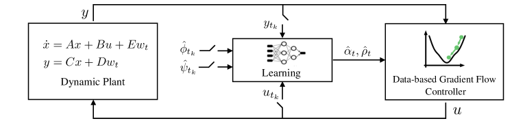
Figure 1: Block diagram of the proposed gradient flow controller with concurrent learning.

Input: $\hat{\alpha}_{t_{0}},\hat{\rho}_{t_{0}}$ based on recorded data; gain $\eta>0$, number of basis functions $N$, $M$.

For all $t\geq t_{0}$:

# Learning

if  new data point $(\hat{\phi}(u_{t}),u_{t})$ obtained  then

      

$$\hat{\alpha}_{t} \leftarrow\operatorname{parameter-learning}(\{(\hat{\phi}_{t_{k}},u_{t_{k}})\}_{t_{k}\leq t})$$ (2a)

if  new data point $(\hat{\psi}(y_{t}),y_{t})$ obtained then

      

$$\hat{\rho}_{t} \leftarrow\operatorname{parameter-learning}(\{(\hat{\psi}_{t_{j}},y_{t_{j}})\}_{t_{j}\leq t})$$ (2b)

end if

# Feedback Control

$$\dot{x} =Ax+Bu+Ew_{t},\,\,y=Cx+Dw_{t}$$

$$\dot{u} =-\eta(\nabla b(u)^{\top}\hat{\alpha}_{t}+G^{\top}\nabla d(y)^{\top}\hat{\rho}_{t}).$$ (2c)

Framework 1 Data-based online gradient-flow controller

The proposed scheme is illustrated in Figure 1, and it is described by the pseudo-code in Framework 1 (with $t_{0}$ denoting the initial time). According to the proposed method, an initial estimate of the parameters $\alpha$ and $\rho$ is obtained using recorded data, where $\operatorname{parameter-learning}(\cdot)$ is a map that represents an estimation step; examples of learning methods will be provided in Section 3.2. Since for any time $t\geq t_{0}$ the parameters are updated only when a new functional evaluation is available, we let $t\mapsto\hat{\alpha}_{t}$ and $t\mapsto\hat{\rho}_{t}$ be piece-wise constant right-continuous functions that represent the most up-to-date estimates of $\alpha$ and $\rho$, respectively. We utilize a gradient-flow controller, as shown in (1), where the gain $\eta>0$ induces a time-scale separation between the plant and the controller. Finally, we notice that since the vector field characterizing (1) is piece-wise continuous in time, the initial value problem (1) always admits a local solution that is unique [Khalil(2002), Thm 3.1].

3.1 Main results

In this section, we characterize the transient performance of Framework 1. To this end, let

$$z :=(u-u^{*}_{t},x-x^{*}_{t}), x^{*}_{t} =-A^{\scalebox{0.75}[0.9]{$-$}1}Bu^{*}_{t}-A^{\scalebox{0.75}[0.9]{$-$}1}Ew_{t},$$ (3)

denote the error between the state of (1) and the equilibrium of (2), respectively. In the following, we provide sufficient conditions on $\eta$ and on the estimation errors $\alpha-\hat{\alpha}_{t}$, $\rho-\hat{\rho}_{t}$ so that the interconnection between the plant and the data-based controller (1) is exponentially stable.

The first result is stated for (Case 1), where the functions $\phi$ and $\psi$ are represented by a finite number of basis functions, and we set precisely $N=N_{b}$ and $M=M_{b}$.

Theorem 3.1.

(Control bound for finite number of basis functions) Let Assumptions 1-7 be satisfied, and assume that $N=N_{b}<\infty$ and $M=M_{b}<\infty$. Let $z(t)$ be defined as in (3), with $(u(t),x(t))$ the state of (1). Suppose that the learning errors satisfy,

$$0<\epsilon:=\ell_{u}\sup_{t_{0}\leq\tau\leq t}\|\alpha-\hat{\alpha}_{\tau}\|+\ell_{y}\|G\|^{2}\sup_{t_{0}\leq\tau\leq t}\|\rho-\hat{\rho}_{\tau}\|<\frac{c_{0}}{c_{3}},$$ (4)

where $c_{0}:=s\min\left\{2\mu_{u}\eta,\underline{\lambda}(Q)/\bar{\lambda}(P)\right\},c_{3}:=\eta\max\left\{2\ell\mu_{u}^{-1},4c_{1}^{-1}\|PA^{-1}B\|\right\},$ $c_{1}:=\min\{(1-\theta)\mu_{u}/2,\theta\underline{\lambda}\left(P\right)\},\theta:=\ell_{y}\|G\|\|C\|/(\ell_{y}\|G\|\|C\|+2\|PA^{-1}B\|),$ and $s\in(0,1)$. Suppose further that the controller gain satisfies,

$$0<\eta<\frac{(1-s)^{2}\underline{\lambda}(Q)}{\left(2-s\right)2\|PA^{-1}B\|\ell_{y}\|G\|\|C\|}.$$ (5)

Then there exists $\kappa_{1},\kappa_{2},\kappa_{3}>0$ such that the error $z(t)$ satisfies

$$\|z(t)\|\leq\kappa_{1}e^{-\frac{1}{2}a(t-t_{0})}\|z(t_{0})\|+\kappa_{2}\int_{t_{0}}^{t}e^{-\frac{1}{2}a(t-\tau)}\Delta(\tau)d\tau+\kappa_{3}\int_{t_{0}}^{t}e^{-\frac{1}{2}a(t-\tau)}\|\dot{w}_{\tau}\|d\tau,$$ (6)

for all $t\geq t_{0}\geq 0$, where $a:=c_{0}-\epsilon\,c_{3}$ and $\Delta(\tau):=\|\nabla b(u^{*}_{\tau})\|\|\alpha-\hat{\alpha}_{\tau}\|+\|\nabla d(y^{*}_{\tau})\|\|\rho-\hat{\rho}_{\tau}\|$.

Detailed expressions for the constants $\kappa_{1},\kappa_{2},\kappa_{3}$ are provided in Appendix 6, and the proof of Theorem 3.1 is provided in Appendix 7. Theorem 3.1 asserts that if the worst-case estimation error for the parameters of the cost functions, captured by $\sup_{t_{0}\leq\tau\leq t}\|\alpha-\hat{\alpha}_{\tau}\|$ and $\sup_{t_{0}\leq\tau\leq t}\|\rho-\hat{\rho}_{\tau}\|$, is such that $\epsilon$ satisfies the condition (4), then a sufficiently-small choice of the controller gain $\eta$ guarantees exponential convergence of the state of (1) to a neighborhood of the optimizer $u^{*}_{t}$ of (2) and the corresponding state $x_{t}^{*}$. In particular, the error $z(t)$ is ultimately bounded by two terms: the first depends on the error $\Delta(t)$, which accounts for the estimation error in the function parameters, and the second depends on temporal variability of $w_{t}$ (which affects the dynamics of the plant (1) making the optimizer of (2) time varying). The condition on $\epsilon$ also suggests prerequisites on the “richness” of the recorded data in the sense that they must yield a sufficiently small estimation error.

It is important to notice that $a=c_{0}-\epsilon\,c_{3}$, which characterizes the rate of exponential decay, is proportional to smallest value between the rate of the convergence of the open-loop plant (found in $c_{0}$ as the ratio $\underline{\lambda}(Q)/\bar{\lambda}(P)$ [Khalil(2002), Chapter 4, Theorem 4.10]) and the strong convexity parameter $\mu_{u}$, characterizing the cost function. Moreover, the rate of convergence $a$ is proportional to the controller gain $\eta$ (as described by $c_{0}$ and $c_{3}$), and inversely proportional to the worst-case estimation errors of the parameters of the cost, $\sup_{t_{0}\leq\tau\leq t}\|\alpha-\hat{\alpha}_{\tau}\|$ and $\sup_{t_{0}\leq\tau\leq t}\|\rho-\hat{\rho}_{\tau}\|$.

Remark 1.

(Asymptotic behavior and input-to-state stability) Two important implications follow from the statement of Theorem 3.1 as subcases.

$\bullet$ If $\lim_{t\rightarrow\infty}\Delta(t)=0$ and $\lim_{t\rightarrow\infty}\dot{w}_{t}=0$, then (6) guarantees that $\lim_{t\rightarrow\infty}z(t)=0$, namely, the state of (1) converges (exactly) to the optimizer of (2). See [Khalil(2002), Lemma 9.6].

$\bullet$ If $\operatorname{ess}\sup_{t_{0}\leq\tau\leq t}\|\Delta(\tau)\|<\infty$ and $\operatorname{ess}\sup_{t_{0}\leq\tau\leq t}\|\dot{w}_{\tau}\|<\infty$, then (6) guarantees that

$$\|z(t)\|\leq\kappa_{1}e^{-\frac{1}{2}a(t-t_{0})}\|z(t_{0})\|+2a^{\scalebox{0.75}[0.9]{$-$}1}(\kappa_{2}\operatorname{ess}\sup_{t_{0}\leq\tau\leq t}\|\Delta(\tau)\|+\kappa_{3}\operatorname{ess}\sup_{t_{0}\leq\tau\leq t}\|\dot{w}_{\tau}\|).$$ (7)

It follows that the bound (7) guarantees input-to state stability of (1) (in the sense of [Sontag and Wang(1997), Angeli et al.(2003)Angeli, Sontag, and Wang, Sontag(2022)]) with respect to the inputs $\Delta$ and $\dot{w}_{t}$. $\square$

We now consider (Case 2), where the estimation procedure is affected by a truncation error; that is, when only $N\ll N_{b}$ and $M\ll M_{b}$ basis functions are utilized by the controller. Accordingly, consider the approximated functions $\tilde{\phi}(u)=\sum_{i=1}^{N}\alpha_{i}b_{i}(u)$ and $\tilde{\psi}(y)=\sum_{j=1}^{M}\rho_{j}d_{j}(y)$, and define the two truncation errors for $\phi(u)$ and $\psi(y)$ as $e_{\phi}(u):=\sum_{i=N+1}^{N_{b}}b_{i}(u)\alpha_{i}$ and $e_{\psi}(y):=\sum_{j=M+1}^{M_{b}}d_{j}(y)\rho_{j}$, respectively. We make the following regularity assumptions:

Assumption 8

The approximated functions $\tilde{\phi}(u)$ and $\tilde{\psi}(y)$ are $\ell_{u}^{N}$- and $\ell_{y}^{M}$-smooth for constants $\ell_{u}^{N}\geq 0$ and $\ell_{y}^{M}\geq 0$, respectively.

Assumption 9

The truncation terms $e_{\phi}(u)$ and $e_{\psi}(y)$ have a Lipschitz-continuous gradient with constants $\ell_{u}^{e}\geq 0$ and $\ell_{y}^{e}\geq 0$, respectively.

Assumption 8 is satisfied if the basis functions $\{b_{i}\}_{i=1}^{N}$ and $\{d_{i}\}_{i=1}^{M}$ are strongly smooth. Assumption 9 is a technical condition that is required in our proof; nevertheless, this condition is satisfied for parametric convex models and several non-parametric models; see [Hastie et al.(2009)Hastie, Tibshirani, and Friedman, Bazerque and Giannakis(2013)], and the recent results of [Poveda et al.(2021)Poveda, Benosman, and Vamvoudakis].

We next characterize the controller transient performance in the presence of truncation errors.

Theorem 3.2.

(Stability with function approximation error) Let Assumptions 1-9 be satisfied, and assume that $N<N_{b}$ and $M<M_{b}$ basis functions are utilized in the learning of $\phi$ and $\psi$, respectively. Suppose that

$$0<\epsilon^{\prime}:=\ell_{u}^{N}\sup_{t_{0}\leq\tau\leq t}\|\alpha-\hat{\alpha}_{\tau}\|+\ell_{y}^{M}\|G\|^{2}\sup_{t_{0}\leq\tau\leq t}\|\rho-\hat{\rho}_{\tau}\|+\ell_{u}^{e}+\ell_{y}^{e}\|G\|^{2}<\frac{c_{0}}{c_{3}},$$ (8)

where $s,c_{0},c_{1},c_{3},\theta$ are given in Theorem 3.1 and $\eta$ satisfies (5). Then there exists $\kappa_{1},\kappa_{2},\kappa_{3}>0$ such that the error (3) satisfies

$$\|z(t)\|\leq\kappa_{1}e^{-\frac{1}{2}a^{\prime}(t-t_{0})}\|z(t_{0})\|+\kappa_{2}\int_{t_{0}}^{t}e^{-\frac{1}{2}a^{\prime}(t-\tau)}\Xi(\tau)d\tau+\kappa_{3}\int_{t_{0}}^{t}e^{-\frac{1}{2}a^{\prime}(t-\tau)}\|\dot{w}_{\tau}\|d\tau,$$ (9)

for all $t\geq t_{0}\geq 0$, where $a^{\prime}=c_{0}-\epsilon^{\prime}\,c_{3}$ and $\Xi(\tau):=\|\nabla b(u^{*}_{t})\|\|\alpha-\hat{\alpha}_{\tau}\|+\|G\|\|\nabla d(y^{*}_{t})\|\|\rho-\hat{\rho}_{\tau}\|+\|\nabla e_{\phi}(u^{*}_{t})\|+\|G\|\|\nabla e_{\psi}(y^{*}_{t})\|$.

Detailed expressions for the constants $\kappa_{1},\kappa_{2},\kappa_{3}$ are provided in Appendix 6. By comparison with the definition of $\Delta(t)$, Theorem 3.1, $\Xi(t)$ simultaneously accounts for estimation error and truncation error. We also notice that similar claims to those in Remark 1 can be derived in this case.

3.2 Parameter learning

We present some methods that can be utilized in the step $\operatorname{parameter-learning}(\cdot)$ in Framework 1.

Least Squares Estimator. Consider the function $\phi(u)$. Suppose that at a given time $t\in\mathbb{R}_{\geq 0}$, $K>0$ data points $(\hat{\phi}_{t_{k}},u_{t_{k}})$ are available, with $\{t_{k}\}_{k=1}^{K-1}$ the time instants where data points are received. Let $\hat{\Phi}_{t}:=(\hat{\phi}_{t_{1}},\ldots,\hat{\phi}_{t_{K}})$ be a vector collecting the functional evaluations received up to time $t$, and $B_{t}\in\mathbb{R}^{K\times N}$ be a matrix with rows the regression vectors $\{b(u_{t_{k}})^{\top},k=1,\ldots,K\}$. Given these data points, the ordinary least squares (LS) method determines a solution to the following optimization problems; see, e.g., [Kay(1993), Hastie et al.(2009)Hastie, Tibshirani, and Friedman, Beck(2017)]:

if $$K\geq N \hat{\alpha}_{t}=\arg\min_{\alpha\in\mathbb{R}^{N}}~{}~{}\|\hat{\Phi}_{t}-B_{t}\alpha\|^{2}, \text{ if $K<N$:}\quad\hat{\alpha}_{t}=\arg \min_{\alpha\in\mathbb{R}^{N},~{}\text{s.t.:~{}}\hat{\Phi}_{t}=B_{t}\alpha}~{}~{}\|\alpha\|^{2}.$$:

The above optimization problems admit a unique closed-form solution given by $\hat{\alpha}_{t}=B_{t}^{\dagger}\hat{\Phi}_{t}$, where $B_{t}^{\dagger}$ denotes the Moore-Penrose inverse of $B_{t}$. Moreover, the resulting approximation error admits a closed-form expression given by $\|B_{t}\hat{\alpha}_{t}-\hat{\Phi}_{t}\|^{2}=\|(I-B_{t}B_{t}^{\dagger})\hat{\Phi}_{t}\|^{2}$, which can be interpreted by noting that $(I-B_{t}B_{t}^{\dagger})$ is the orthogonal projector onto the null space of $B_{t}^{\mathsf{T}}$.

A similar procedure can be utilized for the function $\psi$; in particular, we let $\hat{\Psi}_{t}:=(\hat{\psi}_{t_{1}},\ldots,\hat{\psi}_{t_{K}})$ be a vector collecting the functional evaluations of $\psi$ received up to time $t$, and we define the matrix $D_{t}:=(d(y_{t_{1}})^{\top},\dots,d(y_{t_{K}})^{\top})$. Then, the LS yields the estimate $\hat{\rho}_{t}=D_{t}^{\dagger}\hat{\Psi}_{t}$.

Recursive Least Squares. To avoid the computation of the Moore-Penrose inverse, one can utilize the recursive LS approach; we refer the reader to [Ljung(1999)] and [Kay(1993)] an overview and for the main equations of the recursive LS. See also [Notarnicola et al.(2021)Notarnicola, Simonetto, Farina, and Notarstefano].

Ridge Regression. Given the data points $(\hat{\Psi}_{t},B_{t})$, the ridge regression involves the solution of the optimization problem $\min_{\alpha\in\mathbb{R}^{N}}\|\hat{\Phi}_{t}-B_{t}\alpha\|^{2}+\lambda_{t}\|\alpha\|^{2}$, where $\lambda_{t}>0$ is a tuning parameter. While this criterion was proposed to alleviate the singularity of $B_{t}^{\top}B_{t}$ when $K<N$ in [Hoerl and Kennard(1970)], the regularization $\lambda_{t}\|\alpha\|^{2}$ can be shown to impose a penalty on the norm of $\alpha$; in fact, for a given $\lambda_{t}>0$, there exists $\nu_{t}>0$ such that the solution of the ridge regression is equivalent to the LS with the constraint $\|\alpha\|\leq\nu_{t}$ as explained by, e.g., [Hastie et al.(2009)Hastie, Tibshirani, and Friedman]. The ridge regression problem admits a unique closed-form solution given by $\hat{\alpha}_{t}=(B_{t}^{\top}B_{t}+\lambda_{t}I)^{-1}B_{t}^{\top}\hat{\Phi}_{t}$, where $I_{N}$ denotes the identity matrix. Similarly, upon receiving the $K$-th data point, the estimate of the vector $\hat{\rho}_{t}$ can be updated as $\hat{\rho}_{t}=(D_{t}^{\top}D_{t}+\lambda_{t}I)^{-1}D_{t}^{\top}\hat{\Psi}_{t}$, where $I_{N}$ denotes the identity matrix. To avoid the matrix inversion, a recursive strategy via the Woodbury matrix identity can be adopted.

Sparse Linear Regression. To select the basis functions that provide a parsimonious representation of the function, one could utilize a sparse liner regression method. This amounts to solving the problem $\min_{\alpha\in\mathbb{R}^{N}}\|\hat{\Phi}_{t}-B_{t}\alpha\|^{2}+\lambda_{t}\|\alpha\|_{1}$, where $\lambda_{t}>0$ is a tuning parameter that promotes sparsity of the vector $\alpha$ as explained in [Tibshirani(1996)]. The solution of the problem can be found in closed form, where the $i$-th entry of $\hat{\alpha}_{t}$ is given by is $\hat{\alpha}_{i,t}=\max\{|z_{i,t}|-\lambda_{t},0\}\textrm{sgn}(z_{i,t})$, with $z_{t}=(B_{t}^{\top}B_{t})^{-1}B_{t}^{\top}\hat{\Phi}_{t}$ and where $\textrm{sgn}(\cdot)$ is the sign function.

4 Numerical Verification

In this section, we numerically verify the proposed Framework 1 in two cases: (i) with constant disturbance $w_{t}$, and (ii) with time-varying disturbance. As an illustrative example, we utilize the LS estimator described in Section 3.2. We consider the cost functions $\phi(u)=\frac{1}{2}u^{\top}\Upsilon u+\upsilon^{\top}u+r$ and $\psi(y)=\frac{1}{2}\|Gu+Hw_{t}-\xi\|^{2}$, where $\Upsilon\in\mathbb{R}^{m\times m}$ is a symmetric positive-definite matrix, $\upsilon\in\mathbb{R}^{m}$ is positive element-wise, $r\in\mathbb{R}$ is positive, and $\xi\in\mathbb{R}^{p}$ is a reference output of the system.

Since the functions are convex and quadratic, we consider the basis expansion in Example (2.2) (see also [Notarnicola et al.(2021)Notarnicola, Simonetto, Farina, and Notarstefano]); notice that to get orthonomal basis functions, we remove the lower-triangular part of $\Upsilon$ and we impose that $\Upsilon_{ij}=\Upsilon_{ji}$, for $i\neq j$. For illustration purposes, we consider a case where we estimate $\phi(u)$ (while $\psi(y)$ is known), and we consider the case $m=4$. We generate some of the matrices of the plant and of the cost functions using normally distributed random variables; the values of the matrices are reported in Appendix 8. We utilize four data points $\{(u,\phi(u))\}$ as recorded data; as such, the LS is under-determined at the start of the algorithm. During the execution of the algorithm, we simulate the arrival of new data points by using a Poisson clock. The gain of the controller satisfies the condition outlines in Theorem 3.1.

Figure 2 illustrates the evolution of the error $z(t)$, defined in (3), as well as the theoretical bound provided in equation (6) of Theorem 3.1. Figure 2(a) illustrated the case where the disturbance is constant; new functional evaluations are received at the times marked with vertical black dotted lines. The theoretical bound depends on the estimation error, and it exhibits step changes when a new data point is received; the theoretical bound appears to be tight in the numerical simulation.

Figure 2(a) illustrated the case where the disturbance is time varying; in this case, the bound is affected by both the estimation error and $\|\dot{w}_{t}\|$. In both cases, the numerical trajectory exhibits an exponential convergence up to an asymptotic error. The asymptotic error is affected by the error in the estimation of the parameters and the variability of the disturbance.

(a)

(b)

Figure 2: Evolution of the error $\|z(t)\|$, and theoretical bounds provided in Theorem 3.1. Left: constant disturbance, $\dot{w}_{t}=0$. Right: time-varying disturbance, $\dot{w}_{t}\neq 0$. Vertical black dotted lines represent time instants where functional evaluations are received.

5 Conclusions

We proposed a data-enabled gradient-flow controller to regulate an LTI dynamical system to the minimizer of an unknown functions. The controller is aided by a learning method that estimates the unknown costs from functional evaluations; to this end, appropriate basis expansion representations (either parametric or non-parametric) are utilized. We established sufficient conditions on the estimation error and the controller gain to ensure that the error between the optimizer of the problem and the state of the closed-loop system is ultimately bounded; the error bound accounts for the functional estimation errors and the temporal variability of the unknown disturbance. Future works will look at learning methods such as concurrent learning dynamics and neural networks.

This work was supported by the National Science Foundation (NSF) through the Awards CMMI 2044946 and CAREER 1941896.

6 Complete Results for Theorems 3.1 and 3.2

Here we provide more details on the Theorems 3.1 and 3.2. In the main results, we define the constants $\kappa_{1},\kappa_{2}$, $\kappa_{3}>0$ as:

$$\kappa_{1} :=\sqrt{\frac{c_{1}}{c_{2}}}$$ (10)

$$\kappa_{2} :=\frac{c_{4}}{2\sqrt{c_{1}}}$$ (11)

$$\kappa_{3} :=\frac{c_{5}}{2\sqrt{c_{1}}}$$ (12)

where:

$$c_{1} :=\min\left\{\frac{(1-\theta)}{\eta}\frac{\mu_{u}}{2},\frac{\theta}{\eta}\underline{\lambda}\left(P\right)\right\},$$ (13)

$$c_{2} :=\max\left\{\frac{(1-\theta)}{\eta}\frac{\ell}{2},\frac{\theta}{\eta}\bar{\lambda}(P)\right\},$$ (14)

$$c_{4} :=\sqrt{\eta}\max\left\{\ell\sqrt{\frac{2}{\mu_{u}}},\frac{2\|PA^{-1}B\|}{\sqrt{\underline{\lambda}(P)}}\right\},$$ (15)

$$c_{5} :=\frac{2\|P^{\top}A^{-1}E\|}{\sqrt{\eta}\sqrt{\underline{\lambda}(P)}}.$$ (16)

7 Proofs of the Main Results

To prove our main results, we combine arguments from perturbation theory and singular perturbation theory (respectively, [Khalil(2002), Ch. 9, Sec. 9.3] and [Khalil(2002), Ch. 11, S. 11.5]). First, we derive a Lyapunov function inspired from [Khalil(2002), Thm. 11.3, Lem. 9.3] and we characterize the choices of the controller gain $\eta$ that guarantee stability of the controlled system in the absence of disturbances. Second, we use Lemma 9.5 [Khalil(2002), Sec. 9.3] to characterize the transient behavior behavior of the controller error in the presence of disturbances.

7.1 Notation for Cost Functions

Given $\phi(u)=\sum_{i=1}^{N}\alpha_{i}b_{i}(u)+\sum_{i=N+1}^{N_{b}}b_{i}(u)\alpha_{i}$, $N<\infty$, with basis functions $b_{i}:\mathbb{R}^{m}\rightarrow\mathbb{R}$, denote the column vectors $\alpha:=[\alpha_{1},\alpha_{2},\dots,\alpha_{N}]^{\top}$, $b(u):=[b_{1}(u),b_{2}(u),\dots,b_{N}(u)]^{\top}$, and $e_{\phi}(u):=\sum_{i=N+1}^{N_{b}}b_{i}(u)\alpha_{i}$. Then, under Assumption 6 the function $\phi(\cdot)$ can be rewritten as

$$\phi(u)=b(u)^{\top}\alpha+e_{\phi}(u).$$

The gradient of $\phi(u)$ is given by $\nabla\phi(u)=\sum_{i=1}^{N}\alpha_{i}\nabla b_{i}(u)+\nabla e_{\phi}(u)$, and the estimated gradient based on an estimate $\hat{\alpha}_{t}$ of $\alpha$ available at time $t$ is $\nabla\hat{\phi}(u)=\sum_{i=1}^{N}\hat{\alpha}_{i,t}\nabla b_{i}(u)$. Let $\nabla b(u)$ denote the Jacobian of $b(u)$, or:

$$\nabla b:=\left[\begin{array}[]{cccc}\frac{\partial b_{1}}{\partial u_{1}}&\ldots&\ldots&\frac{\partial b_{1}}{\partial u_{m}}\\ \vdots&&&\vdots\\ \frac{\partial b_{N}}{\partial u_{1}}&\ldots&\ldots&\frac{\partial b_{N}}{\partial u_{m}}\end{array}\right].$$

Then, we write the gradient of the true function $\phi$ and the estimated function $\hat{\phi}$, respectively, as,

$$\nabla\phi(u)=\nabla b(u)^{\top}\alpha+\nabla e_{\phi}(u)\text{ and }\nabla\hat{\phi}(u)=\nabla b(u)^{\top}\hat{\alpha}_{t}.$$

Similarly, given $\psi(y)=\sum_{j=1}^{M}\rho_{j}d_{j}(y)+\sum_{j=M+1}^{M_{b}}d_{j}(y)\rho_{j}$, $M<\infty$, with basis functions $d_{j}:\mathbb{R}^{p}\rightarrow\mathbb{R}$, denote the column vectors $\rho:=[\rho_{1},\rho_{2},\dots,\rho_{M}]^{\top}$, $d(y):=[d_{1}(y),d_{2}(y),\dots,d_{M}(y)]^{\top}$, and truncation error $e_{\psi}(y):=\sum_{j=M+1}^{M_{b}}d_{j}(y)\rho_{j}$ to rewrite the cost function as

$$\psi(y)=d(y)^{\top}\rho+e_{\psi}(y).$$

The gradient of $\psi(y)$ is given by $\nabla\psi(y)=\sum_{i=1}^{M}\rho_{i}\nabla d_{i}(y)+\nabla e_{\psi}(y)$, and the estimated gradient based on an estimate $\hat{\rho}_{t}$ of $\rho$ available at time $t$ is $\nabla\hat{\psi}(y)=\sum_{i=1}^{M}\hat{\rho}_{i,t}\nabla d_{i}(y)$. Let $\nabla d(u)$ denote the Jacobian of $d(y)$, namely,

$$\nabla d:=\left[\begin{array}[]{cccc}\frac{\partial d_{1}}{\partial y_{1}}&\ldots&\ldots&\frac{\partial d_{1}}{\partial y_{p}}\\ \vdots&&&\vdots\\ \frac{\partial d_{M}}{\partial y_{1}}&\ldots&\ldots&\frac{\partial d_{M}}{\partial y_{p}}\end{array}\right].$$

Then, we write the gradient of the true function $\psi$ and the estimated function $\hat{\psi}$, respectively, as,

$$\nabla\psi(y)=\nabla d(y)^{\top}\rho+\nabla e_{\psi}(y)\text{ and }\nabla\hat{\psi}(y)=\nabla d(y)^{\top}\hat{\rho}_{t}.$$

We recall that we consider two cases. In (Case 1) the functions $\phi$ and $\psi$ are both represented by a finite number of basis functions, and we set $N=N_{b}$ and $M=M_{b}$ basis functions; in this case, $e_{\phi}(u)=0$ and $e_{\psi}(y)=0$. In (Case 2), we have $N\ll N_{b}$ and $M\ll M_{b}$ (where $N_{b}$ and $M_{b}$ may be large or even $\infty$). In this section, we outline the main proof for case (Case 2); the proof for (Case 1) follows directly, and we will specify relevant modifications whenever needed.

7.2 Perturbed Gradient Flow and Singular-Perturbation Model

Consider the controller, which is based on a perturbed gradient flow:

$$\dot{u}=-\eta\left(\nabla\hat{\phi}(u)+\nabla\hat{\psi}(y)\right)=-\eta\left(\nabla b(u)^{\top}\hat{\alpha}_{t}+\nabla d(y)^{\top}\hat{\rho}_{t}\right).$$ (17)

Rewrite (17) in terms of a nominal term (i.e., the true gradient) and an error term (i.e., the perturbation) by first adding and subtracting the true gradients, $\nabla\phi(u)=\nabla b(u)^{\top}\alpha+\nabla e_{\phi}(u)$ and $\nabla\psi(y)=\nabla d(y)^{\top}\rho+\nabla e_{\psi}(y)$:

$$\dot{u}=-\eta\left(\nabla\phi(u)+\nabla\psi(y)\right)+\eta\left(\nabla b(u)^{\top}(\alpha-\hat{\alpha}_{t})+\nabla d(y)^{\top}(\rho-\hat{\rho}_{t})+\nabla e_{\phi}(u)+\nabla_{\psi}(y)\right).$$

Now, add and subtract $\eta\nabla b(u^{*})^{\top}(\alpha-\hat{\alpha}_{t})+\eta\nabla e_{\phi}(u^{*})$ and $\eta\nabla d(y^{*})^{\top}(\rho-\hat{\rho}_{t})+\eta\nabla e_{\psi}(y^{*})$ to obtain:

$$\dot{u}=-\eta \left\{\nabla\phi(u)+\nabla\psi(y)\right\}+\eta\{\left(\nabla b(u)-\nabla b(u^{*})\right)^{\top}(\alpha-\hat{\alpha}_{t})+(\nabla d(y)-\nabla d(y^{*}))^{\top}(\rho-\hat{\rho}_{t})$$

$$+(\nabla e_{\phi}(u)-\nabla e_{\phi}(u^{*}))+(\nabla e_{\psi}(y)-\nabla e_{\psi}(y^{*}))$$

$$+\nabla b(u^{*})^{\top}(\alpha-\hat{\alpha}_{t})+\nabla d(y^{*})^{\top}(\rho-\hat{\rho}_{t})+\nabla e_{\phi}(u^{*})+\nabla e_{\psi}(y^{*})\}.$$ (18)

This representation is in line with the model of [Khalil(2002), Ch. 9, Ch. 11], in which the use of a nominal and error term is inspired by Ch. 9, and the use of controller gain, $\eta$, follows singular perturbation theory. With this representation, the interconnection between plant and controller can be rewritten as:

$$\begin{split}\dot{x}&=Ax+Bu+Ew_{t},\\ y&=Cx+Dw_{t},\\ \dot{u}&=-\eta\left\{\nabla\phi(u)+\nabla\psi(y)\right\}+\eta\{\left(\nabla b(u)-\nabla b(u^{*})\right)^{\top}(\alpha-\hat{\alpha}_{t})+(\nabla d(y)-\nabla d(y^{*}))^{\top}(\rho-\hat{\rho}_{t})\\ &~{}~{}~{}~{}~{}~{}~{}~{}~{}~{}~{}~{}~{}~{}~{}~{}~{}+(\nabla e_{\phi}(u)-\nabla e_{\phi}(u^{*}))+(\nabla e_{\psi}(y)-\nabla e_{\psi}(y^{*}))\\ &~{}~{}~{}~{}~{}~{}~{}~{}~{}~{}~{}~{}~{}~{}~{}~{}~{}+\nabla b(u^{*})^{\top}(\alpha-\hat{\alpha}_{t})+\nabla d(y^{*})^{\top}(\rho-\hat{\rho}_{t})+\nabla e_{\phi}(u^{*})+\nabla e_{\psi}(y^{*})\}.\end{split}$$ (19)

7.3 Change of Variables

We begin by performing a change of variables to shift the equilibrium point of the plant to the origin. For any $w_{t}$, let $x_{eq}$ be the (unique) equilibrium of (1), and define $x^{\prime}:=x-x_{eq}=x-(-A^{-1}Bu-A^{-1}Ew_{t})$ to obtain

$$\dot{x}=\dot{x}^{\prime}+\dot{x}_{eq}=A(x^{\prime}+x_{eq})+Bu+Ew_{t}\implies\dot{x}^{\prime}+\dot{x}_{eq}=Ax^{\prime}+Ax_{eq}+Bu+Ew_{t},$$

and

$$\dot{x}^{\prime}+\frac{\partial x_{eq}}{\partial u}\dot{u}+\frac{\partial x_{eq}}{\partial w_{t}}\dot{w}_{t}=Ax^{\prime}+(-Bu-Ew_{t})+Bu+Ew_{t}\implies\dot{x}^{\prime}=Ax+A^{-1}B\dot{u}+A^{-1}E\dot{w}_{t}.$$

The system $\dot{x}^{\prime}=Ax+A^{-1}B\dot{u}+A^{-1}E\dot{w}_{t}$ is the so-called “boundary-layer system;” see [Khalil(2002), Chapter 11].

Next, we rewrite the controller dynamics in the new variables. Recall that at equilibrium, $y=Gu+Hw_{t}$, with $G=-CA^{-1}B$ and $H=D-CA^{-1}E$. Also, we know that $y=Cx+Dw_{t}.$ Use these facts for the following change of variables:

$$\psi(y) =\psi(Cx+Dw_{t})=\psi(C(x^{\prime}+x_{eq})+Dw_{t})$$

$$=\psi(Cx^{\prime}-CA^{-1}Bu-CA^{-1}Ew_{t}+Dw_{t})$$

$$=\psi(Cx^{\prime}+Gu+Hw_{t}).$$

Then, the gradient can be written as $G^{\top}\nabla\psi(Cx^{\prime}+Gu+Hw_{t})$. For brevity, hereafter we write $y$ to mean $y=Cx^{\prime}+Gu+Hw_{t}$ and $y^{*}=Cx^{\prime}+Gu^{*}+Hw_{t}$ for the error terms in the controller With these changes of variables, the controller can be written as:

$$\dot{u} =-\eta(\nabla\phi(u)+G^{\top}\nabla\psi(Cx^{\prime}+Gu-Hw_{t}))$$

$$~{}~{}~{}~{}~{}~{}~{}~{}~{}~{}~{}~{}~{}~{}~{}~{}~{}+\eta\{\left(\nabla b(u)-\nabla b(u^{*})\right)^{\top}(\alpha-\hat{\alpha}_{t})+(G^{\top}\nabla d(y)-G^{\top}\nabla d(y^{*}))^{\top}(\rho-\hat{\rho}_{t})$$

$$~{}~{}~{}~{}~{}~{}~{}~{}~{}~{}~{}~{}~{}~{}~{}~{}~{}+(\nabla e_{\phi}(u)-\nabla e_{\phi}(u^{*}))+(G^{\top}\nabla e_{\psi}(y)-G^{\top}\nabla e_{\psi}(y^{*}))$$

$$~{}~{}~{}~{}~{}~{}~{}~{}~{}~{}~{}~{}~{}~{}~{}~{}~{}+\nabla b(u^{*})^{\top}(\alpha-\hat{\alpha}_{t})+\nabla d(y^{*})^{\top}(\rho-\hat{\rho}_{t})+\nabla e_{\phi}(u^{*})+G^{\top}\nabla e_{\psi}(y^{*})\}$$

where we have again a nominal gradient flow and the perturbation. This system is the “reduced system” in our singular-perturbation setup; see  [Khalil(2002), Chapter 11].

In what follows, we denote in compact form

$$m(u,x) :=-\nabla\phi(u)-G^{\top}\nabla\psi(Cx+Dw_{t}),$$

$$n(u,x) :=Ax+Bu+Ew_{t},$$

$$e(u,y) :=(\nabla b(u)-\nabla b(u^{*}))^{\top}(\alpha-\hat{\alpha}_{t})+(G^{\top}\nabla d(y)-G^{\top}\nabla d(y^{*}))^{\top}(\rho-\hat{\rho}_{t})$$

$$~{}~{}+(\nabla e_{\phi}(u)+\nabla e_{\phi}(u^{*}))+(G^{\top}\nabla e_{\psi}(y)-G^{\top}\nabla e_{\psi}(y^{*}))$$

$$~{}~{}+\nabla b(u^{*})^{\top}(\alpha-\hat{\alpha}_{t})+G^{\top}\nabla d(y^{*})^{\top}(\rho+\hat{\rho}_{t})+\nabla e_{\phi}(u^{*})+G^{\top}\nabla e_{\psi}(y^{*}).$$

Accordingly, the dynamics in the new variables read as:

$$\dot{x}^{\prime} =n(u,x^{\prime}+x_{eq})-\eta\frac{\partial x_{eq}}{\partial u}\dot{u}-\frac{\partial x_{eq}}{\partial w_{t}}\dot{w}_{t}, \dot{u} =\eta\,m(u,x^{\prime}+x_{eq})+\eta\,e(u,y).$$

7.4 Lyapunov Functions and Bounds

For the boundary-layer system, propose the following Lyapunov function:

$$W(x^{\prime})=x^{\prime\top}Px^{\prime}$$ (20)

where, for any positive definite matrix $Q\in R^{n\times n},$ $P\succ 0$ is the solution to the Lyapunov equation $A^{\top}P+PA=-Q$ as in Assumption 1. Notice that (20) satisfies the following quadratic bounds:

$$\underline{\lambda}(P)\|x^{\prime}\|^{2}\leq W(x^{\prime})\leq\bar{\lambda}(P)\|x^{\prime}\|^{2}.$$ (21)

For the reduced system, we utilize the Lyapunov function:

$$V(t,u;w)=\phi(u)-\phi(u^{*})+\psi(Gu+Hw_{t})-\psi(Gu^{*}+Hw_{t}).$$ (22)

Note that (22) satisfies the bounds:

$$\frac{\mu_{u}}{2}\|u-u^{*}\|^{2}\leq V(u)\leq\frac{\ell_{u}+\ell_{y}\|G\|^{2}}{2}\|u-u^{*}\|^{2}.$$ (23)

then, combining (20) and (22), we obtain the composite Lyapunov function

$$\nu(t,u,x^{\prime};w)=(1-\theta)\frac{1}{\eta}V(t,u;w)+\theta\frac{1}{\eta}W(x^{\prime}),$$ (24)

where $\theta\in(0,1)$. In the following, we utilize the compact notation $z=(u-u^{*},x^{\prime})$.

Quadratic bounds on the composite Lyapunov function. Next, we derive quadratic bounds on the composite Lyapunov function. Since the function $\phi+\psi$ is $\mu_{u}$-strongly convex in $u$, it holds that:

$$(1-\theta)\frac{1}{\eta}\frac{\mu_{u}}{2}\|u-u^{*}\|^{2}+\frac{\theta}{\eta}\underline{\lambda}(P)\|x^{\prime}\|^{2}\leq\nu(t,z;w)$$

where $u^{*}$ is the unique minimizer of (2). Moreover, since the composite function $\phi(u)+\psi(Gu+Hw_{t})$ is Lipschitz-smooth with parameter $\ell_{u}+\|G\|^{2}\ell_{y}$, using the Descent Lemma [Beck(2014), Lemma 4.22] we get:

$$\nu(t,z;w)\leq(1-\theta)\frac{1}{\eta}\frac{(\ell_{u}+\|G\|^{2}\ell_{y})}{2}\|u-u^{*}\|^{2}+\frac{\theta}{\eta}\bar{\lambda}(P)\|x^{\prime}\|^{2}.$$

Setting $c_{1}$ $:=\min\{(1-\theta)\frac{1}{\eta}\frac{\mu_{u}}{2},\frac{\theta}{\eta}\underline{\lambda}\left(P\right)\}$ and $c_{2}:=\max\{(1-\theta)\frac{1}{\eta}\frac{(\ell_{u}+\|G\|^{2}\ell_{y})}{2},\frac{\theta}{\eta}\bar{\lambda}(P)\}$, obtain the quadratic bounds,

$$c_{1}\|z\|^{2}\leq\nu(t,z;w)\leq c_{2}\|z\|^{2}.$$ (25)

Bound for the derivatives of the Lyapunov function along the trajectories of the system. Consider the derivative of the composite Lyapunov function along the trajectories of the closed loop system:

$$\dot{\nu}(t,z;w)=(1-\theta)\frac{1}{\eta}\dot{V}(t,u;w)+\theta\frac{1}{\eta}\dot{W}(x^{\prime}).$$ (26)

Consider the first term on the right hand side of (26); the derivative can be calculated as:

$$(1-\theta)\frac{1}{\eta}\dot{V}(t,u;w) =\frac{(1-\theta)}{\eta}\frac{\partial V}{\partial u}^{\top}\dot{u}$$

$$=\frac{(1-\theta)}{\eta}\frac{\partial V}{\partial u}^{\top} \eta(m(u,x^{\prime}+x_{eq})+e)$$

$$=(1-\theta)\frac{\partial V}{\partial u}^{\top} (m(u,x^{\prime}+x_{eq})+e)+(1-\theta)\frac{\partial V}{\partial u}^{\top}m(u,x_{eq})-(1-\theta)\frac{\partial V}{\partial u}^{\top}m(u,x_{eq})$$

$$=(1-\theta)\frac{\partial V}{\partial u}^{\top} \left(m(u,x^{\prime}+x_{eq})-m(u,x_{eq})\right)+(1-\theta)\frac{\partial V}{\partial u}^{\top}m(u,x_{eq})+(1-\theta)\frac{\partial V}{\partial u}^{\top}e.$$

By expanding each term:

$$(1-\theta)\frac{\partial V}{\partial u}^{\top} \left(m(u,x^{\prime}+x_{eq})-m(u,x_{eq})\right)=$$

$$=(1-\theta)(\nabla\phi(u)-\nabla\phi(u^{*})+G^{\top}\nabla\psi(Gu+Hw_{t})-G^{\top}\nabla\psi(Gu^{*}+Hw_{t}))$$

$$~{}~{}\times(-\nabla\phi(u)-G^{\top}\nabla\psi(Cx^{\prime}+Gu+Hw_{t})+\nabla\phi(u)+G^{\top}\nabla\psi(Gu+Hw_{t}))$$

$$=(1-\theta)(\nabla\phi(u)+G^{\top}\nabla\psi(Gu+Hw))^{\top}$$

$$~{}~{}\times(-G^{\top}\nabla\psi(Cx^{\prime}+Gu+Hw_{t})+G^{\top}\nabla\psi(Gu+Hw_{t}))$$

$$\leq(1-\theta)\|G\|\|\nabla\phi(u)+G^{\top}\nabla\psi(Gu+Hw_{t})\|$$

$$~{}~{}\times\|\nabla\psi(Cx^{\prime}+Gu+Hw_{t})-\nabla\psi(Gu+Hw_{t})\|$$

$$\leq(1-\theta)\ell_{y}\|G\|\|C\|\|\nabla\phi(u)+G^{\top}\nabla\psi(Gu+Hw_{t})\|\|x^{\prime}\|,$$

$$(1-\theta)\frac{\partial V}{\partial u}^{\top} m(u,x_{eq})=$$

$$=(1-\theta)(\nabla\phi(u)-\nabla\phi(u^{*})+G^{\top}\nabla\psi(Gu+Hw_{t})-G^{\top}\nabla\psi(Gu^{*}+Hw_{t}))^{\top}$$

$$~{}~{}\times(-\nabla\phi(u)-G^{\top}\nabla\psi(Gu+Hw_{t}))$$

$$=(1-\theta)(\nabla\phi(u)+G^{\top}\nabla\psi(Gu+Hw_{t}))^{\top}\times(-\nabla\phi(u)-G^{\top}\nabla\psi(Gu+Hw_{t}))$$

$$=-(1-\theta)\|\nabla\phi(u)+G^{\top}\nabla\psi(Gu+Hw_{t})\|^{2},$$

and

$$(1-\theta)\frac{\partial V}{\partial u}^{\top} e=$$

$$=(1-\theta)(\nabla\phi(u)-\nabla\phi(u^{*})+G^{\top}\nabla\psi(Gu+Hw_{t})-G^{\top}\nabla\psi(Gu^{*}+Hw_{t}))^{\top}$$

$$~{}~{}\times\{(\nabla b(u)-\nabla b(u^{*}))^{\top}(\alpha-\hat{\alpha}_{t})+\nabla b(u^{*})^{\top}(\alpha-\hat{\alpha}_{t})$$

$$~{}~{}~{}~{}+(G^{\top}\nabla d(y)-G^{\top}\nabla d(y^{*}))^{\top}(\rho-\hat{\rho}_{t})+G^{\top}\nabla d(y^{*})^{\top}(\rho-\hat{\rho}_{t})$$

$$~{}~{}~{}~{}+(\nabla e_{\phi}(u^{*})-\nabla e_{\phi}(u^{*}))+(G^{\top}\nabla e_{\psi}(y)-G^{\top}\nabla e_{\psi}(y^{*}))+\nabla e_{\phi}(u^{*})+G^{\top}\nabla e_{\psi}(y^{*})\}$$

$$=(1-\theta)(\nabla\phi(u)+G^{\top}\nabla\psi(Gu+Hw_{t}))^{\top}$$

$$~{}~{}\times\{(\nabla b(u)-\nabla b(u^{*}))^{\top}(\alpha-\hat{\alpha}_{t})+\nabla b(u^{*})^{\top}(\alpha-\hat{\alpha}_{t})$$

$$~{}~{}~{}~{}+(G^{\top}\nabla d(y)-G^{\top}\nabla d(y^{*}))^{\top}(\rho-\hat{\rho}_{t})+G^{\top}\nabla d(y^{*})^{\top}(\rho-\hat{\rho}_{t})$$

$$~{}~{}~{}~{}+(\nabla e_{\phi}(u^{*})-\nabla e_{\phi}(u^{*}))+(G^{\top}\nabla e_{\psi}(y)-G^{\top}\nabla e_{\psi}(y^{*}))+\nabla e_{\phi}(u^{*})+G^{\top}\nabla e_{\psi}(y^{*})\}$$

$$\leq(1-\theta)\|\nabla\phi(u)+G^{\top}\nabla\psi(Gu+Hw_{t})\|$$

$$~{}~{}\times\|(\nabla b(u)-\nabla b(u^{*}))^{\top}(\alpha-\hat{\alpha}_{t})+\nabla b(u^{*})^{\top}(\alpha-\hat{\alpha}_{t})$$

$$~{}~{}~{}~{}+(G^{\top}\nabla d(y)-G^{\top}\nabla d(y^{*}))^{\top}(\rho-\hat{\rho}_{t})+G^{\top}\nabla d(y^{*})^{\top}(\rho-\hat{\rho}_{t})$$

$$~{}~{}~{}~{}+(\nabla e_{\phi}(u^{*})-\nabla e_{\phi}(u^{*}))+(G^{\top}\nabla e_{\psi}(y)-G^{\top}\nabla e_{\psi}(y^{*}))+\nabla e_{\phi}(u^{*})+G^{\top}\nabla e_{\psi}(y^{*})\|$$

$$\leq(1-\theta)\left(\ell_{u}+\ell_{y}\|G\|^{2}\right)\|u-u^{*}\|$$

$$~{}~{}\times\{\|\nabla b(u)-\nabla b(u^{*})\|\|\alpha-\hat{\alpha}_{t}\|+\|G\|\|\nabla d(y)-\nabla d(y^{*})\|\|\rho-\hat{\rho}_{t}\|$$

$$~{}~{}~{}~{}~{}~{}~{}+\|\nabla b(u^{*})\|\|\alpha-\hat{\alpha}_{t}\|+\|G\|\|\nabla d(y^{*})\|\|\rho-\hat{\rho}_{t}\|$$

$$~{}~{}~{}~{}+\|\nabla e_{\phi}(u^{*})-\nabla e_{\phi}(u^{*})\|+\|G\|\|\nabla e_{\psi}(y)-\nabla e_{\psi}(y^{*})\|+\|\nabla e_{\phi}(u^{*})\|+\|G\|\|\nabla e_{\psi}(y^{*})\|\}$$

$$=(1-\theta)\left(\ell_{u}+\ell_{y}\|G\|^{2}\right)\|u-u^{*}\|$$

$$~{}~{}\times\{(\ell_{u}^{N}\|\alpha-\hat{\alpha}_{t}\|+\ell_{y}^{M}\|G\|^{2}\|\rho-\hat{\rho}_{t}\|+\ell_{u}^{e}+\ell_{y}^{e}\|G\|^{2})\|u-u^{*}\|$$

$$~{}~{}~{}~{}+\|\nabla b(u^{*})\|\|\alpha-\hat{\alpha}_{t}\|+\|G\|\|\nabla d(y^{*})\|\|\rho-\hat{\rho}_{t}\|+\|\nabla e_{\phi}(u^{*})\|+\|G\|\|\nabla e_{\psi}(y^{*})\|\}$$

$$=(1-\theta)\left(\ell_{u}+\ell_{y}\|G\|^{2}\right)\left(\ell_{u}^{N}\|\alpha-\hat{\alpha}_{t}\|+\ell_{y}^{M}\|G\|^{2}\|\rho-\hat{\rho}_{t}\|+\ell_{u}^{e}+\ell_{y}^{e}\|G\|^{2}\right)\|u-u^{*}\|^{2}$$

$$~{}~{}~{}+(1-\theta)\left(\ell_{u}+\ell_{y}\|G\|^{2}\right)\{\|\nabla b(u^{*})\|\|\alpha-\hat{\alpha}_{t}\|+\|G\|\|\nabla d(y^{*})\|\|\rho-\hat{\rho}_{t}\|$$

$$~{}~{}~{}~{}~{}~{}~{}~{}~{}~{}~{}~{}~{}~{}~{}~{}~{}~{}~{}~{}~{}~{}~{}~{}~{}~{}~{}~{}~{}~{}~{}~{}~{}~{}~{}~{}~{}~{}~{}~{}~{}~{}~{}~{}~{}~{}~{}~{}~{}+\|\nabla e_{\phi}(u^{*})\|+\|G\|\|\nabla e_{\psi}(y^{*})\|\}\|u-u^{*}\|.$$

For the second term on the right hand size of (26), calculate:

$$\frac{\theta}{\eta}\dot{W}(x^{\prime}) =\frac{\theta}{\eta}\frac{\partial W}{\partial x^{\prime}}^{\top}\dot{x}^{\prime}$$

$$=\frac{\theta}{\eta}\frac{\partial W}{\partial x^{\prime}}^{\top}\left(n(u,x^{\prime}+x_{eq})-\eta\frac{\partial x_{eq}}{\partial u}\dot{u}-\frac{\partial x_{eq}}{\partial w_{t}}\dot{w}_{t}\right)$$

$$=\frac{\theta}{\eta}\frac{\partial W}{\partial x^{\prime}}^{\top}\left(n(u,x^{\prime}+x_{eq})-\eta\frac{\partial x_{eq}}{\partial u}(m(u,x^{\prime}+x_{eq})+e)-\frac{\partial x_{eq}}{\partial w_{t}}\dot{w}_{t}\right)$$

$$=\frac{\theta}{\eta}\frac{\partial W}{\partial x^{\prime}}^{\top}n(u,x^{\prime}+x_{eq})-\frac{\theta}{\eta}\eta\frac{\partial W}{\partial x^{\prime}}^{\top}\frac{\partial x_{eq}}{\partial u}m(u,x^{\prime}+x_{eq})-\frac{\theta}{\eta}\eta\frac{\partial W}{\partial x^{\prime}}^{\top}\frac{\partial x_{eq}}{\partial u}e-\frac{\theta}{\eta}\frac{\partial W}{\partial x^{\prime}}^{\top}\frac{\partial x_{eq}}{\partial w_{t}}\dot{w}_{t}$$

$$=\frac{\theta}{\eta}\frac{\partial W}{\partial x^{\prime}}^{\top}n(u,x^{\prime}+x_{eq})-\theta\frac{\partial W}{\partial x^{\prime}}^{\top}\frac{\partial x_{eq}}{\partial u}m(u,x^{\prime}+x_{eq})-\theta\frac{\partial W}{\partial x^{\prime}}^{\top}\frac{\partial x_{eq}}{\partial u}e-\frac{\theta}{\eta}\frac{\partial W}{\partial x^{\prime}}^{\top}\frac{\partial x_{eq}}{\partial w_{t}}\dot{w}_{t}.$$

Analyzing each term, one has that:

$$\frac{\theta}{\eta}\frac{\partial W}{\partial x^{\prime}}^{\top}n(u,x^{\prime}+x_{eq}) =-\frac{\theta}{\eta}x^{\prime\top}Qx^{\prime}\leq-\frac{\theta}{\eta}\underline{\lambda}(Q)\|x^{\prime}\|^{2},$$

$$-\theta\frac{\partial W}{\partial x^{\prime}}^{\top}\frac{\partial x_{eq}}{\partial u}m(u,x^{\prime}+x_{eq}) =\theta(2x^{\prime\top}P^{\top})(-A^{-1}B)(\nabla\phi(u)+G^{\top}\nabla\psi(Cx^{\prime}+Gu+Hw_{t}))$$

$$=\theta(2x^{\prime\top}P^{\top})(-A^{-1}B)(\nabla\phi(u)+G^{\top}\nabla\psi(Gu+Hw_{t})$$

$$~{}~{}~{}~{}~{}+G^{\top}\nabla\psi(Cx^{\prime}+Gu+Hw_{t})-G^{\top}\nabla\psi(Gu+Hw_{t}))$$

$$\leq\theta 2\|PA^{-1}B\|\|x^{\prime}\|\{\|\nabla\phi(u)+G^{\top}\nabla\psi(Gu+Hw_{t})\|$$

$$~{}~{}~{}~{}~{}+\|G\|\|\nabla\psi(Cx^{\prime}+Gu+Hw_{t})-\nabla\psi(Gu+Hw_{t})\|\}$$

$$\leq\theta 2\|PA^{-1}B\|\|x^{\prime}\|\{\|\nabla b(u)^{\top}\alpha+G^{\top}\nabla\psi(Gu+Hw_{t})\|+\ell_{y}\|G\|\|C\|\|x^{\prime}\|\}$$

$$=\theta 2\|PA^{-1}B\|\|\nabla\phi(u)+G^{\top}\nabla\psi(Gu+Hw_{t})\|\|x^{\prime}\|$$

$$~{}~{}~{}+\theta 2\|PA^{-1}B\|\ell_{y}\|G\|\|C\|\|x^{\prime}\|^{2},$$

$$-\theta\frac{\partial W}{\partial x^{\prime}}^{\top}\frac{\partial x_{eq}}{\partial u}e =\theta(2x^{\prime\top}P^{\top})(-A^{-1}B)$$

$$~{}~{}\times\{(\nabla b(u)-\nabla b(u^{*}))^{\top}(\alpha-\hat{\alpha}_{t})+\nabla b(u^{*})^{\top}(\alpha-\hat{\alpha}_{t})$$

$$~{}~{}~{}~{}+(G^{\top}\nabla d(y)-G^{\top}\nabla d(y^{*}))^{\top}(\rho-\hat{\rho}_{t})+G^{\top}\nabla d(y^{*})^{\top}(\rho-\hat{\rho}_{t})$$

$$~{}~{}~{}~{}+(\nabla e_{\phi}(u^{*})-\nabla e_{\phi}(u^{*}))+(G^{\top}\nabla e_{\psi}(y)-G^{\top}\nabla e_{\psi}(y^{*}))+\nabla e_{\phi}(u^{*})+G^{\top}\nabla e_{\psi}(y^{*})\}$$

$$\leq\theta 2\|PA^{-1}B\|\|x^{\prime}\|\{\ell_{u}^{N}\|\alpha-\hat{\alpha}_{t}\|\|u-u^{*}\|+\|\nabla b(u^{*})\|\|\alpha-\hat{\alpha}_{t}\|$$

$$~{}~{}~{}+\ell_{y}^{M}\|G\|^{2}\|\rho-\rho_{t}\|\|u-u^{*}\|+\|G\|\|\nabla d(y^{*})\|\|\rho-\hat{\rho}_{t}\|$$

$$~{}~{}~{}+(\ell_{u}^{e}+\ell_{y}^{e}\|G\|^{2})\|u-u^{*}\|+\|\nabla e_{\phi}(u)\|+\|G\|\|\nabla e_{\psi}(y^{*})\|\}$$

$$=\theta 2\|PA^{-1}B\|\left(\ell_{u}^{N}\|\alpha-\hat{\alpha}_{t}\|+\ell_{y}^{M}\|G\|^{2}\|\rho-\hat{\rho}_{t}\|+\ell_{u}^{e}+\ell_{y}^{e}\|G\|^{2}\right)\|u-u^{*}\|\|x^{\prime}\|$$

$$~{}~{}~{}+\theta 2\|PA^{-1}B\|\{\|\nabla b(u^{*})\|\|\alpha-\hat{\alpha}_{t}\|+\|G\|\|\nabla d(y^{*})\|\|\rho-\hat{\rho}_{t}\|$$

$$~{}~{}~{}~{}~{}~{}~{}~{}~{}~{}~{}~{}~{}~{}~{}~{}~{}~{}~{}~{}~{}~{}~{}~{}~{}~{}~{}~{}~{}~{}~{}~{}~{}~{}~{}~{}~{}~{}~{}~{}~{}~{}~{}~{}~{}~{}~{}~{}~{}+\|\nabla e_{\phi}(u^{*})\|+\|G\|\|\nabla e_{\psi}(y^{*})\|\}\|x^{\prime}\|,$$

and

$$-\frac{\theta}{\eta}\frac{\partial W}{\partial x^{\prime}}^{\top}\frac{\partial x_{eq}}{\partial w_{t}}\dot{w}_{t} =\frac{1}{\eta}\theta(2Px^{\prime})^{\top}(-A^{-1}E)\dot{w}_{t}$$

$$\leq\frac{1}{\eta}\theta 2\|PA^{-1}E\|\|x^{\prime}\|\|\dot{w}_{t}\|.$$

By combining the above bounds, (26) can be bounded above as follows:

$$\begin{split}&\dot{\nu}(u,w,x^{\prime})\leq(1-\theta)\{\ell_{y}\|G\|\|C\|\|\nabla\phi(u)+G^{\top}\nabla\psi(Gu+Hw_{t})\|\|x^{\prime}\|\\ &~{}~{}~{}-\|\nabla\phi(u)+G^{\top}\nabla\psi(Gu+Hw_{t})\|^{2}\\ &~{}~{}~{}+(\ell_{u}+\ell_{y}\|G\|^{2})\left(\ell_{u}^{N}\|\alpha-\hat{\alpha}_{t}\|+\ell_{y}^{M}\|G\|^{2}\|\rho-\hat{\rho}_{t}\|+\ell_{u}^{e}+\ell_{y}^{e}\|G\|^{2}\right)\|u-u^{*}\|^{2}\\ &~{}~{}~{}+(\ell_{u}+\ell_{y}\|G\|^{2})\left(\|\nabla b(u^{*})\|\|\alpha-\hat{\alpha}_{t}\|+\|G\|\|\nabla d(y^{*})\|\|\rho-\hat{\rho}_{t}\|+\|\nabla e_{\phi}(u^{*})\|+\|G\|\|\nabla e_{\psi}(y^{*})\|\right)\|u-u^{*}\|\}\\ &-\frac{\theta}{\eta}\underline{\lambda}(Q)\|x^{\prime}\|^{2}\\ &~{}~{}~{}+\theta 2\|PA^{-1}B\|\|\nabla\phi(u)+G^{\top}\nabla\psi(Gu+Hw_{t})\|\|x^{\prime}\|+\theta 2\|PA^{-1}B\|\ell_{y}\|G\|\|C\|\|x^{\prime}\|^{2}\\ &~{}~{}~{}+\theta 2\|PA^{-1}B\|\left(\ell_{u}^{N}\|\alpha-\hat{\alpha}_{t}\|+\ell_{y}^{M}\|G\|^{2}\|\rho-\hat{\rho}_{t}\|+\ell_{u}^{e}+\ell_{y}^{e}\|G\|^{2}\right)\|x^{\prime}\|\|u-u^{*}\|\\ &~{}~{}~{}~{}+\theta 2\|PA^{-1}B\|\left(\|\nabla b(u^{*})\|\|\alpha-\hat{\alpha}_{t}\|+\|G\|\|\nabla d(y^{*})\|\|\rho-\hat{\rho}_{t}\|+\|\nabla e_{\phi}(u^{*})\|+\|G\|\|\nabla e_{\psi}(y^{*})\|\right)\|x^{\prime}\|\\ &~{}~{}~{}~{}~{}+\frac{1}{\eta}\theta 2\|PA^{-1}E\|\|x^{\prime}\|\|\dot{w}_{t}\|.\end{split}$$ (27)

7.5 Deriving Conditions on the Controller Gain

We will now utilize the bounds (21), (23) to identify sufficient conditions on the controller gain to guarantee strong decrease of the Lyapunov function.

To this aim, we will show that the bound (LABEL:eq:derivativeLyapunovUpperB) can be rewritten as

$$\dot{\nu} \leq-\Omega^{\top}\Lambda\Omega-c_{0}\nu+(1-\theta)\{(\ell_{u}+\ell_{y}\|G\|^{2})\left(\ell_{u}^{N}\|\alpha-\hat{\alpha}_{t}\|+\ell_{y}^{M}\|G\|^{2}\|\rho-\hat{\rho}_{t}\|+\ell_{u}^{e}+\ell_{y}^{e}\|G\|^{2}\right)\|u-u^{*}\|^{2}$$

$$+(\ell_{u}+\ell_{y}\|G\|^{2})\left(\|\nabla b(u^{*})\|\|\alpha-\hat{\alpha}_{t}\|+\|G\|\|\nabla d(y^{*})\|\|\rho-\hat{\rho}_{t}\|+\|\nabla e_{\phi}(u^{*})\|+\|G\|\|\nabla e_{\psi}(y^{*})\|\right)\|u-u^{*}\|)\}$$

$$~{}~{}~{}+\theta 2\|PA^{-1}B\|\left(\ell_{u}^{N}\|\alpha-\hat{\alpha}_{t}\|+\ell_{y}^{M}\|G\|^{2}\|\rho-\hat{\rho}_{t}\|+\ell_{u}^{e}+\ell_{y}^{e}\|G\|^{2}\right)\|x^{\prime}\|\|u-u^{*}\|$$

$$~{}~{}~{}~{}+\theta 2\|PA^{-1}B\|\left(\|\nabla b(u^{*})\|\|\alpha-\hat{\alpha}_{t}\|+\|G\|\|\nabla d(y^{*})\|\|\rho-\hat{\rho}_{t}\|+\|\nabla e_{\phi}(u^{*})\|+\|G\|\|\nabla e_{\psi}(y^{*})\|\right)\|x^{\prime}\|$$

$$~{}~{}~{}~{}~{}+\frac{1}{\eta}\theta 2\|PA^{-1}E\|\|x^{\prime}\|\|\dot{w}_{t}\|,$$

where $\Lambda$ is a $2\times 2$ positive definite matrix and

$$\begin{split}\Omega(x^{\prime},u)=\begin{bmatrix}\|\nabla\phi(u)+G^{\top}\nabla\psi(Gu+Hw_{t})\|\\ \|x^{\prime}\|\end{bmatrix}.\end{split}$$ (28)

Notice that, in this case, $\Omega(x^{\prime},u)^{\top}\Lambda\Omega(x^{\prime},u)=0$ if and only if $(x^{\prime},u)=(0,u^{*}_{t})$ (namely, at the optimizer) and $\Omega(x^{\prime},u)^{\top}\Lambda\Omega(x^{\prime},u)>0$ otherwise.

To this aim, let $s\in(0,1)$, and re-organize (LABEL:eq:derivativeLyapunovUpperB) as:

$$\begin{split}&\dot{\nu}(u,w,x^{\prime})\leq(1-\theta)\{\ell_{y}\|G\|\|C\|\|\nabla\phi(u)+G^{\top}\nabla\psi(Gu+Hw_{t})\|\|x^{\prime}\|\\ &~{}~{}~{}-(1-s)\|\nabla\phi(u)+G^{\top}\nabla\psi(Gu+Hw_{t})\|^{2}-s\|\nabla\phi(u)+G^{\top}\nabla\psi(Gu+Hw_{t})\|^{2}\\ &~{}~{}~{}+(\ell_{u}+\ell_{y}\|G\|^{2})\left(\ell_{u}^{N}\|\alpha-\hat{\alpha}_{t}\|+\ell_{y}^{M}\|G\|^{2}\|\rho-\hat{\rho}_{t}\|+\ell_{u}^{e}+\ell_{y}^{e}\|G\|^{2}\right)\|u-u^{*}\|^{2}\\ &~{}~{}~{}+(\ell_{u}+\ell_{y}\|G\|^{2})\left(\|\nabla b(u^{*})\|\|\alpha-\hat{\alpha}_{t}\|+\|G\|\|\nabla d(y^{*})\|\|\rho-\hat{\rho}_{t}\|+\|\nabla e_{\phi}(u^{*})\|+\|G\|\|\nabla e_{\psi}(y^{*})\|\right)\|u-u^{*}\|\}\\ &-(1-s)\frac{\theta}{\eta}\underline{\lambda}(Q)\|x^{\prime}\|^{2}-s\frac{\theta}{\eta}\underline{\lambda}(Q)\|x^{\prime}\|^{2}\\ &~{}~{}~{}+\theta 2\|PA^{-1}B\|\|\nabla\phi(u)+G^{\top}\nabla\psi(Gu+Hw_{t})\|\|x^{\prime}\|+\theta 2\|PA^{-1}B\|\ell_{y}\|G\|\|C\|\|x^{\prime}\|^{2}\\ &~{}~{}~{}+\theta 2\|PA^{-1}B\|\left(\ell_{u}^{N}\|\alpha-\hat{\alpha}_{t}\|+\ell_{y}^{M}\|G\|^{2}\|\rho-\hat{\rho}_{t}\|+\ell_{u}^{e}+\ell_{y}^{e}\|G\|^{2}\right)\|x^{\prime}\|\|u-u^{*}\|\\ &~{}~{}~{}~{}+\theta 2\|PA^{-1}B\|\left(\|\nabla b(u^{*})\|\|\alpha-\hat{\alpha}_{t}\|+\|G\|\|\nabla d(y^{*})\|\|\rho-\hat{\rho}_{t}\|+\|\nabla e_{\phi}(u^{*})\|+\|G\|\|\nabla e_{\psi}(y^{*})\|\right)\|x^{\prime}\|\\ &~{}~{}~{}~{}~{}+\frac{1}{\eta}\theta 2\|PA^{-1}E\|\|x^{\prime}\|\|\dot{w}_{t}\|.\end{split}$$ (29)

In particular, consider the terms $s\|\nabla\phi(u)+G^{\top}\nabla\psi(Gu+Hw_{t})\|^{2}$ and $s\frac{\theta}{\eta}\underline{\lambda}(Q)\|x^{\prime}\|^{2}$ in (LABEL:eq:derivativeLyapunovUpperB2). For the first term, utilize the PL inequality to obtain,

$$-s(1-\theta) \|\nabla\phi(u)+G^{\top}\nabla\psi(Gu+Hw_{t})\|^{2}\leq$$

$$~{}~{}~{}-s2(1-\theta)\mu_{u}\|\phi(u)-\phi(u^{*})+\psi(Gu+Hw_{t})-\psi(Gu^{*}+Hw_{t})\|$$

$$=-s2(1-\theta)\mu_{u}(\phi(u)-\phi(u^{*})+\psi(Gu+Hw_{t})-\psi(Gu^{*}+Hw_{t})$$

$$=-s2(1-\theta)\mu_{u}V.$$

For the second term, calculate

$$\dot{W}(x^{\prime})=-x^{\prime\top}Qx^{\prime}\leq-\frac{\underline{\lambda}(Q)}{\bar{\lambda}(P)}\|x^{\prime}\|^{2}=-\frac{\underline{\lambda}(Q)}{\bar{\lambda}(P)}W(x^{\prime}).$$

Then the second term simplifies to,

$$-s\frac{\theta}{\eta}\underline{\lambda}(Q)\|x^{\prime}\|^{2} \leq-s\frac{\theta}{\eta}\frac{\underline{\lambda}(Q)}{\bar{\lambda}(P)}W(x^{\prime}).$$

Together, these give,

$$\begin{split}-s(1-\theta)&\|\nabla\phi(u)+G^{\top}\nabla\psi(Gu+Hw_{t})\|^{2}-s\frac{\theta}{\eta}\underline{\lambda}(Q)\|x^{\prime}\|^{2}\\ &\leq-s(1-\theta)2\mu_{u}V-s\frac{\theta}{\eta}\frac{\underline{\lambda}(T)}{\bar{\lambda}(P)}W\\ &\leq\min\left\{s2\mu_{u}\eta,s\frac{\underline{\lambda}(Q)}{\bar{\lambda}(P)}\right\}\nu:=c_{0}\nu.\end{split}$$ (30)

To obtain the quadratic form $\Omega(x^{\prime},u)^{\top}\Lambda\Omega(x^{\prime},u)$, define the following coefficients:

$$\alpha_{1} :=(1-s),$$

$$\alpha_{2} :=(1-s)\underline{\lambda}(Q),$$

$$\beta_{1} :=\ell_{y}\|G\|\|C\|,$$

$$\beta_{2} :=2\|PA^{-1}B\|.$$

Then, using terms in (LABEL:eq:derivativeLyapunovUpperB2), one can build $\Lambda$ as

$$\Lambda =\left(\begin{array}[]{ll}(1-\theta)\alpha_{1}&-\frac{1}{2}[(1-\theta)\beta_{1}+\theta\beta_{2}]\\ -\frac{1}{2}[(1-\theta)\beta_{1}+\theta\beta_{2}]&\theta[\frac{\alpha_{2}}{\eta}-\beta_{1}\beta_{2}]\end{array}\right)$$

Matrix $\Lambda$ is positive definite if and only if its principal minors are positive. This yields the following condition on $\eta$:

$$[(1-\theta)\alpha_{1}][\theta\left(\frac{\alpha_{2}}{\eta}-\beta_{1}\beta_{2}\right)] >\frac{1}{4}[(1-\theta)\beta_{1}+\theta\beta_{2}]^{2}$$

$$\alpha_{1}[\frac{\alpha_{2}}{\eta}-\beta_{1}\beta_{2}] >\frac{1}{4\theta(1-\theta)}[(1-\theta)\beta_{1}+\theta\beta_{2}]^{2}$$

$$\alpha_{1}\frac{\alpha_{2}}{\eta} >\frac{1}{4\theta(1-\theta)}[(1-\theta)\beta_{1}+\theta\beta_{2}]^{2}+\alpha_{1}\beta_{1}\beta_{2},$$

and, thus,

$$\eta<\frac{\alpha_{1}\alpha_{2}}{\frac{1}{4\theta(1-\theta)}[(1-\theta)\beta_{1}+\theta\beta_{2}]^{2}+\alpha_{1}\beta_{1}\beta_{2}}.$$ (31)

The right hand side of (31) is a concave function of $\theta$ and, by maximizing with respect to $\theta$, we have that the maximum is obtained at

$$\theta^{*}=\frac{\beta_{1}}{\beta_{1}+\beta_{2}},$$

which gives

$$\eta^{*}=\frac{\alpha_{1}\alpha_{2}}{(\beta_{1}\beta_{2})(1+\alpha_{1})}.$$

7.6 Analysis of the Learning Error and Derivation of the Main Result

Finally, we will show that the time-derivative of the Lyapunov function can be bounded as

$$\dot{\nu}\leq-\Omega(x^{\prime},u)^{\top}\Lambda\Omega(x^{\prime},u)-c_{0}\nu+c_{3}\gamma(t)\nu+\left(c_{4}\delta(t)+c_{5}\|\dot{w}_{t}\|\right)\sqrt{\nu}.$$

To this aim, recall that $z:=(u-u^{*},x^{\prime})$. We will use the inequality $\|u-u^{*}\|+\|x^{\prime}\|\leq\sqrt{2}\|z\|$.

We begin by using (23)-(21), to obtain $\|u-u^{*}\|^{2}\leq\frac{2}{\mu_{u}}V$ and $\|x^{\prime}\|^{2}\leq\frac{W}{\underline{\lambda}(P)}$. Further, by using $\nu:=(1-\theta)\frac{1}{\eta}V+\frac{\theta}{\eta}W,$ we have that $V\leq\frac{\eta}{(1-\theta)}\nu$ and $\sqrt{V}\leq\frac{\sqrt{\eta}}{\sqrt{(1-\theta)}}\sqrt{\nu}.$ Using these facts, we can calculate the following bounds:

(a)

$$(1-\theta)(\ell_{u}+\ell_{y}\|G\|^{2}) \left(\ell_{u}^{N}\|\alpha-\hat{\alpha}_{t}\|+\ell_{y}^{M}\|G\|^{2}\|\rho-\hat{\rho}_{t}\|+\ell_{u}^{e}+\ell_{y}^{e}\|G\|^{2}\right)\|u-u^{*}\|^{2}$$

$$\leq\frac{2}{\mu_{u}}(1-\theta)(\ell_{u}+\ell_{y}\|G\|^{2})\left(\ell_{u}^{N}\|\alpha-\hat{\alpha}_{t}\|+\ell_{y}^{M}\|G\|^{2}\|\rho-\hat{\rho}_{t}\|+\ell_{u}^{e}+\ell_{y}^{e}\|G\|^{2}\right)V(u)$$ (32)

(b) with $\kappa:=(1-\theta)(\ell_{u}+\ell_{y}\|G\|^{2})(\|\nabla b(u^{*})\|\|\alpha-\hat{\alpha}_{t}\|$ $+\|G\|\|\nabla d(y^{*})\|\|\rho-\hat{\rho}_{t}\|+\|\nabla e_{\phi}(u^{*})\|+\|G\|\|\nabla e_{\psi}(y^{*})\|)$ for brevity,

$$\kappa\|u-u^{*}\|\leq\kappa\sqrt{\frac{2}{\mu_{u}}}\sqrt{V(u)}.$$ (33)

(c)

$$2\theta\|PA^{-1}B\| \left(\ell_{u}^{N}\|\alpha-\hat{\alpha}_{t}\|+\ell_{y}^{M}\|G\|^{2}\|\rho-\hat{\rho}_{t}\|+\ell_{u}^{e}+\ell_{y}^{e}\|G\|^{2}\right)\|x^{\prime}\|\|u-u^{*}\|$$

$$\leq 4\theta\|PA^{-1}B\|\left(\ell_{u}^{N}\|\alpha-\hat{\alpha}_{t}\|+\ell_{y}^{M}\|G\|^{2}\|\rho-\hat{\rho}_{t}\|+\ell_{u}^{e}+\ell_{y}^{e}\|G\|^{2}\right)\|z\|^{2}$$

$$\leq 4\frac{\theta}{c_{1}}\|PA^{-1}B\|\left(\ell_{u}^{N}\|\alpha-\hat{\alpha}_{t}\|+\ell_{y}^{M}\|G\|^{2}\|\rho-\hat{\rho}_{t}\|+\ell_{u}^{e}+\ell_{y}^{e}\|G\|^{2}\right)\nu$$

$$\leq\frac{4}{c_{1}}\|PA^{-1}B\|\left(\ell_{u}^{N}\|\alpha-\hat{\alpha}_{t}\|+\ell_{y}^{M}\|G\|^{2}\|\rho-\hat{\rho}_{t}\|+\ell_{u}^{e}+\ell_{y}^{e}\|G\|^{2}\right)\nu$$ (34)

since $\theta\in(0,1)$.

(d) with $\kappa^{\prime}:=2\theta\|PA^{-1}B\|(\|\nabla b(u^{*})\|\|\alpha-\hat{\alpha}_{t}\|$ $+\|G\|\|\nabla d(y^{*})\|\|\rho-\hat{\rho}_{t}\|+\|\nabla e_{\phi}(u^{*})\|+\|G\|\|\nabla e_{\psi}(y^{*})\|)$ for brevity,

$$\kappa^{\prime}\|x^{\prime}\|\leq\kappa^{\prime}\frac{\sqrt{W}}{\sqrt{\underline{\lambda}(P)}}.$$ (35)

And, (e)

$$\frac{\theta}{\eta}2\|P^{\top}A^{-1}E\|\|\dot{w}_{t}\|\|x^{\prime}\|\leq\frac{\theta}{\eta}2\|P^{\top}A^{-1}E\|\|\dot{w}_{t}\|\frac{\sqrt{W}}{\sqrt{\underline{\lambda}(P)}}.$$ (36)

Define

$$\gamma(t) :=\ell_{u}^{N}\|\alpha-\hat{\alpha}_{t}\|+\ell_{y}^{M}\|G\|^{2}\|\rho-\hat{\rho}_{t}\|+\ell_{u}^{e}+\ell_{y}^{e}\|G\|^{2},$$

$$\delta(t) :=\|\nabla b(u^{*})\|\|\alpha-\hat{\alpha}_{t}\|+\|G\|\|\nabla d(y^{*})\|\|\rho-\hat{\rho}_{t}\|+\|\nabla e_{\phi}(u^{*})\|+\|G\|\|\nabla e_{\psi}(y^{*})\|.$$ (37)

For (32), obtain a bound with $\nu$ as:

$$(1-\theta)(\ell_{u}+\ell_{y}\|G\|^{2})\gamma(t)\frac{2}{\mu_{u}}V \leq(\ell_{u}+\ell_{y}\|G\|^{2})\gamma(t)\frac{2\eta}{\mu_{u}}\nu.$$

From the second inequality (33), similarly obtain:

$$(1-\theta)(\ell_{u}+\ell_{y}\|G\|^{2})\delta(t)\sqrt{\frac{2}{\mu_{u}}}\sqrt{V} \leq\sqrt{(1-\theta)}(\ell_{u}+\ell_{y}\|G\|^{2})\delta(t)\sqrt{\frac{2}{\mu_{u}}}\sqrt{\eta}\sqrt{\nu}$$

$$\leq(\ell_{u}+\ell_{y}\|G\|^{2})\delta(t)\sqrt{\frac{2}{\mu_{u}}}\sqrt{\eta}\sqrt{\nu}.$$

The third term remains as-is because it is already bounded above by $\nu$. For the fourth term, obtain:

$$2\theta\|PA^{-1}B\|\delta(t)\frac{\sqrt{W}}{\sqrt{\underline{\lambda}(P)}} \leq 2\sqrt{\theta}\|PA^{-1}B\|\delta(t)\frac{\sqrt{\nu}}{\sqrt{\underline{\lambda}(P)}}\sqrt{\eta}$$

$$\leq 2\|PA^{-1}B\|\delta(t)\sqrt{\nu}\frac{\sqrt{\eta}}{\sqrt{\underline{\lambda}(P)}}.$$

Similarly, we bound the term due to the time-varying disturbance $w_{t}$ as,

$$\frac{\theta}{\eta}2\|P^{\top}A^{-1}E\|\|\dot{w}_{t}\|\frac{\sqrt{W}}{\sqrt{\underline{\lambda}(P)}} \leq\frac{\theta}{\eta}2\|P^{\top}A^{-1}E\|\|\dot{w}_{t}\|\frac{\sqrt{\eta}}{\sqrt{\underline{\lambda}(P)}}\sqrt{\nu}$$

$$\leq\frac{2\|P^{\top}A^{-1}E\|}{\sqrt{\eta}\sqrt{\underline{\lambda}(P)}}\|\dot{w}_{t}\|\sqrt{\nu}.$$

Excluding $\gamma(t)$ and $\delta(t)$, group the terms above in front of $\eta$ and $\sqrt{\eta}$ and define:

$$c_{3}:=\max\left\{(\ell_{u}+\ell_{y}\|G\|^{2})\frac{2\eta}{\mu_{u}},\|PA^{-1}B\|\frac{4}{c_{1}}\right\}$$

$$\text{ and }c_{4}:=\sqrt{\eta}\max\left\{(\ell_{u}+\ell_{y}\|G\|^{2})\sqrt{\frac{2}{\mu_{u}}},\|PA^{-1}B\|\frac{2}{\sqrt{\underline{\lambda}(P)}}\right\}.$$

For the term dealing with $\|\dot{w}_{t}\|$, similarly define:

$$c_{5}:=\frac{2\|P^{\top}A^{-1}E\|}{\sqrt{\eta}\sqrt{\underline{\lambda}(P)}}.$$

In summary,

$$\begin{split}\gamma(t)&:=\ell_{u}^{N}\|\alpha-\hat{\alpha}_{t}\|+\ell_{y}^{M}\|G\|^{2}\|\rho-\hat{\rho}_{t}\|+\ell_{u}^{e}+\ell_{y}^{e}\|G\|^{2},\\ \delta(t)&:=\|\nabla b(u^{*})\|\|\alpha-\hat{\alpha}_{t}\|+\|G\|\|\nabla d(y^{*})\|\|\rho-\hat{\rho}_{t}\|+\|\nabla e_{\phi}(u^{*})\|+\|G\|\|\nabla e_{\psi}(y^{*})\|,\\ c_{0}&:=s\min\left\{2\mu_{u}\eta,\frac{\underline{\lambda}(Q)}{\bar{2}\lambda(P)}\right\},\\ c_{1}&:=\min\left\{(1-\theta)\frac{1}{\eta}\frac{\mu_{u}}{2},\frac{\theta}{\eta}\underline{\lambda}\left(P\right)\right\},\\ c_{2}&:=\max\left\{(1-\theta)\frac{1}{\eta}\frac{(\ell_{u}+\|G\|^{2}\ell_{y})}{2},\frac{\theta}{\eta}\bar{\lambda}(P)\right\},\\ c_{3}&:=\max\left\{(\ell_{u}+\ell_{y}\|G\|^{2})\frac{2\eta}{\mu_{u}},\|PA^{-1}B\|\frac{4}{c_{1}}\right\},\\ c_{4}&:=\sqrt{\eta}\max\left\{(\ell_{u}+\ell_{y}\|G\|^{2})\sqrt{\frac{2}{\mu_{u}}},\|PA^{-1}B\|\frac{2}{\sqrt{\underline{\lambda}(P)}}\right\},\\ c_{5}&:=\frac{2\|P^{\top}A^{-1}E\|}{\sqrt{\eta}\sqrt{\underline{\lambda}(P)}}.\end{split}$$ (38)

Altogether, our analysis bounds $\dot{\nu}$ as,

$$\dot{\nu}\leq-\Omega(x^{\prime},u)^{\top}\Lambda\Omega(x^{\prime},u)-c_{0}\nu+c_{3}\gamma(t)\nu+\left(c_{4}\delta(t)+c_{5}\|\dot{w}_{t}\|\right)\sqrt{\nu}.$$ (39)

We have derived sufficient conditions on $\eta$ so that $\Lambda$ is positive definite; consequently, $\Omega(x^{\prime},u)^{\top}\Lambda\Omega(x^{\prime},u)>0$ must hold and (39) can be further bounded as:

$$\dot{\nu}\leq-\left(c_{0}-c_{3}\gamma(t)\right)\nu+\left(c_{4}\delta(t)+c_{5}\|\dot{w}_{t}\|\right)\sqrt{\nu}.$$ (40)

The following analysis for (40) is inspired by [Khalil(2002), Section 9.3]. First, apply a change of variables $\nu^{\prime}:=\sqrt{\nu}$. Then,

$$\dot{\nu}^{\prime}\leq-\frac{1}{2}\left(c_{0}-c_{3}\gamma(t)\right)\nu^{\prime}+\frac{1}{2}\left(c_{4}\delta(t)+c_{5}\|\dot{w}_{t}\|\right).$$

Let $\Phi(t,t_{0}):=e^{-\frac{1}{2}c_{0}(t-t_{0})+\frac{c_{3}}{2}\int_{t_{0}}^{t}\gamma(\tau)d\tau},$ for a given $t_{0}\geq 0$. By the Comparison Lemma [Khalil(2002), Section 3.4, Section 9.3],

$$\dot{\nu}^{\prime}\leq\Phi(t,t_{0})\nu^{\prime}(t_{0})+\frac{c_{4}}{2}\int_{t_{0}}^{t}\Phi(t,\tau)\delta(\tau)d\tau+\frac{c_{5}}{2}\int_{t_{0}}^{t}\Phi(t,\tau)\|\dot{w}_{\tau}\|d\tau.$$

By (25),

$$\|z(t)\|\leq\sqrt{\frac{c_{2}}{c_{1}}}\Phi(t,t_{0})\|z(t_{0})\|+\frac{c_{4}}{2\sqrt{c_{1}}}\int_{t_{0}}^{t}\Phi(t,\tau)\delta(\tau)d\tau+\frac{c_{5}}{2\sqrt{c_{1}}}\int_{t_{0}}^{t}\Phi(t,\tau)\|\dot{w}_{\tau}\|d\tau.$$ (41)

Note that the errors $\|\alpha-\hat{\alpha}_{t}\|$ and $\|\rho-\hat{\rho}_{t}\|$ within $\gamma(t)$ and $\delta(t)$ are piece-wise constant. Thus, for any $K,K^{\prime}\in\mathbb{N}$, we bound $\gamma(t)$ as:

$$\sum_{i=0}^{K} \ell_{u}^{N}\|\alpha-\hat{\alpha}_{t_{i-1}}\|(t_{i}-t_{i-1})+\sum_{i=0}^{K^{\prime}}\ell_{y}^{M}\|G\|^{2}\|\rho-\hat{\rho}_{t_{i-1}}\|(t_{i}-t_{i-1})$$

$$\leq\underbrace{\left(\ell_{u}^{N}\sup_{t_{0}\leq t\leq\tau}\left\{\|\alpha-\hat{\alpha}_{\tau}\|\right\}+\ell_{y}^{M}\|G\|^{2}\sup_{t_{0}\leq\tau\leq t}\left\{\|\rho-\hat{\rho}_{\tau}\|\right\}+\ell_{u}^{e}+\ell_{y}^{e}\|G\|^{2}\right)}_{:=\epsilon^{\prime}}(t-t_{0}).$$ (42)

In (40), we must ensure that $-c_{0}\nu+c_{3}\gamma(t)\nu<0$. Using (42), we impose the condition

$$\epsilon^{\prime}<\frac{c_{0}}{c_{3}}.$$

Finally, defining $a^{\prime}:=\frac{1}{2}\left(c_{0}-\epsilon^{\prime}c_{3}\right)>0$, we obtain,

$$\|z(t)\|\leq\sqrt{\frac{c_{2}}{c_{1}}}\|z(t_{0})\|e^{-a^{\prime}(t-t_{0})}+\frac{c_{4}}{2\sqrt{c_{1}}}\int_{t_{0}}^{t}e^{-a^{\prime}(t-\tau)}\delta(\tau)d\tau+\frac{c_{5}}{2\sqrt{c_{1}}}\int_{t_{0}}^{t}e^{-a^{\prime}(t-\tau)}\|\dot{w}_{\tau}\|d\tau.$$ (43)

Theorem 3.2 follows by noting that $\Xi(t)=\delta(t)$.

To show the result of Theorem 3.1, the same steps can be used upon setting $\nabla e_{\phi}(u)=0$, $\nabla e_{\psi}(y)=0$, $\nabla e_{\phi}(u^{*})=0$, and $\nabla e_{\psi}(y^{*})=0$ in (18), since there is no truncation error in Theorem 3.1. This lead to the re-definition of $\gamma(t)$ and $\delta(t)$ as $\gamma(t):=\ell_{u}\|\alpha-\hat{\alpha}_{t}\|+\ell_{y}\|G\|^{2}\|\rho-\hat{\rho}_{t}\|$ and $\delta(t):=\|\nabla b(u^{*})\|\|\alpha-\hat{\alpha}_{t}\|+\|G\|\|\nabla d(y^{*})\|\|\rho-\hat{\rho}_{t}\|$, respectively.

8 Numerical Values for Simulation

Here, we provide the exact matrices used to generate Figure 2.

$$A =\begin{bmatrix}-2.7527&-0.6944&-2.8952&-0.7989\\ 1.2008&-4.3397&-1.7097&-0.6025\\ -0.2198&-1.0665&-5.1494&0.3043\\ -2.8886&1.922&2.7361&-3.8897\end{bmatrix},B=C=D=E=\begin{bmatrix}1&0&0&0\\ 0&1&0&0\\ 0&0&1&0\\ 0&0&0&1\end{bmatrix},$$

$$\Upsilon =\begin{bmatrix}6.095&0.6234&0.1468&-0.9387\\ 0.6234&6.4595&-1.0145&1.0203\\ 0.1468&-1.0145&7.0719&0.7042\\ -0.9387&1.0203&0.7042&4.5038\end{bmatrix},\upsilon=\begin{bmatrix}0.0201\\ 1.4908\\ 1.2373\\ 1.8092\end{bmatrix},r=-0.1504,$$

$$Q =\begin{bmatrix}3.994&-1.1602&-0.1978&-0.9408\\ -1.1602&4.0145&-0.3114&-0.8189\\ -0.1978&-0.3114&5.9914&-1.8039\\ -0.9408&-0.8189&-1.8039&5.3419\end{bmatrix},P=\begin{bmatrix}1.3220&0.3400&-0.3819&-0.9667\\ 0.3400&0.7413&-0.3188&-0.4261\\ -0.3819&-0.3188&0.6745&0.1771\\ -0.9667&-0.4261&0.1771&1.3186\\ \end{bmatrix}.$$

The matrices $Q,P$ are used in the Lyapunov function for the boundary layer system as shown in Appendix 7.

References

- [Angeli et al.(2003)Angeli, Sontag, and Wang] D. Angeli, E. D. Sontag, and Y. Wang. Input-to-state stability with respect to inputs and their derivatives. International Journal of Robust and Nonlinear Control: IFAC-Affiliated Journal, 13(11):1035–1056, 2003.
- [Ariyur and Krstić(2003)] K. B. Ariyur and M. Krstić. Real-time optimization by extremum-seeking control. John Wiley & Sons, 2003.
- [Bazerque and Giannakis(2013)] J. Bazerque and G. B. Giannakis. Nonparametric basis pursuit via sparse kernel-based learning: A unifying view with advances in blind methods. IEEE Signal Processing Magazine, 30(4):112–125, 2013.
- [Beck(2014)] A. Beck. Introduction to Nonlinear Optimization: Theory, Algorithms, and Applications with MATLAB. MOS-SIAM Series on Optimization, Technion-Israel Institute of Technology, Kfar Saba, Israel, 2014.
- [Beck(2017)] A. Beck. First Order Methods in Optimization. MOS-SIAM Series on Optimization, Tel-Aviv University, Tel-Aviv, Israel, 2017.
- [Bianchin et al.(2020)Bianchin, Poveda, and Dall’Anese] G. Bianchin, J. I. Poveda, and E. Dall’Anese. Online optimization of switched LTI systems using continuous-time and hybrid accelerated gradient flows. arXiv preprint arXiv:2008.03903, 2020.
- [Bianchin et al.(2021a)Bianchin, Cortés, Poveda, and Dall’Anese] G. Bianchin, J. Cortés, J. I. Poveda, and E. Dall’Anese. Time-varying optimization of LTI systems via projected primal-dual gradient flows. IEEE Trans. on Control of Networked Systems, 2021a.
- [Bianchin et al.(2021b)Bianchin, Dall’Anese, Poveda, Jacobson, Carlton, and Buchwald] G. Bianchin, E. Dall’Anese, J. I. Poveda, D. Jacobson, E. J. Carlton, and A. G. Buchwald. Planning a return to normal after the COVID-19 pandemic: Identifying safe contact levels via online optimization. arXiv preprint arXiv:2109.06025, 2021b.
- [Bourgin et al.(2019)Bourgin, Peterson, Reichman, Russell, and Griffiths] D. D. Bourgin, J. C. Peterson, D. Reichman, S. J. Russell, and T. L. Griffiths. Cognitive model priors for predicting human decisions. In International Conference on Machine Learning, pages 5133–5141, 2019.
- [Brunner et al.(2012)Brunner, Dürr, and Ebenbauer] F. D. Brunner, H.-B. Dürr, and C. Ebenbauer. Feedback design for multi-agent systems: A saddle point approach. In IEEE Conf. on Decision and Control, pages 3783–3789, 2012.
- [Chowdhary and Johnson(2010)] G. Chowdhary and E. Johnson. Concurrent learning for convergence in adaptive control without persistency of excitation. In IEEE Conf. on Decision and Control, pages 3674–3679. IEEE, 2010.
- [Chowdhary et al.(2013)Chowdhary, Yucelen, Mühlegg, and Johnson] G. Chowdhary, T. Yucelen, M. Mühlegg, and E. N. Johnson. Concurrent learning adaptive control of linear systems with exponentially convergent bounds. International Journal of Adaptive Control and Signal Processing, 27(4):280–301, 2013.
- [Colombino et al.(2020)Colombino, Dall’Anese, and Bernstein] M. Colombino, E. Dall’Anese, and A. Bernstein. Online optimization as a feedback controller: Stability and tracking. IEEE Trans. on Control of Network Systems, 7(1):422–432, 2020.
- [Cothren et al.(2021)Cothren, Bianchin, and Dall’Anese] L. Cothren, G. Bianchin, and E Dall’Anese. Data-enabled gradient flow as feedback controller: Regulation of linear dynamical systems to minimizers of unknown functions (extended version). arXiv preprint, 2021. https://arxiv.org/abs/2112.01652.
- [Davison(1976)] E. Davison. The robust control of a servomechanism problem for linear time-invariant multivariable systems. IEEE Trans. on Automatic Control, 21(1):25–34, 1976.
- [Devraj and Meyn(2017)] A. M Devraj and S. P Meyn. Zap Q-learning. In Proceedings of the 31st International Conference on Neural Information Processing Systems, pages 2232–2241, 2017.
- [Fabiani et al.(2021)Fabiani, Simonetto, and Goulart] F. Fabiani, A. Simonetto, and P. J. Goulart. Learning equilibria with personalized incentives in a class of nonmonotone games. arXiv preprint arXiv:2111.03854, 2021.
- [Gündling et al.(2020)Gündling, Hopp, and Weihe] F. Gündling, F. Hopp, and K. Weihe. Efficient monitoring of public transport journeys. Public Transport, 12(3):631–645, 2020.
- [Hastie et al.(2009)Hastie, Tibshirani, and Friedman] T. Hastie, R. Tibshirani, and J. Friedman. The elements of statistical learning. Springer, 2009.
- [Hauswirth et al.(2021a)Hauswirth, Bolognani, Hug, and Dörfler] A. Hauswirth, S. Bolognani, G. Hug, and F. Dörfler. Timescale separation in autonomous optimization. IEEE Trans. on Automatic Control, 66(2):611–624, 2021a.
- [Hauswirth et al.(2021b)Hauswirth, Bolognani, Hug, and Dörfler] A. Hauswirth, S. Bolognani, G. Hug, and F. Dörfler. Optimization algorithms as robust feedback controllers. arXiv preprint arXiv:2103.11329, 2021b.
- [Hirata et al.(2014)Hirata, Hespanha, and Uchida] K. Hirata, J. P. Hespanha, and K. Uchida. Real-time pricing leading to optimal operation under distributed decision makings. In Proc. of American Control Conf., Portland, OR, June 2014.
- [Hoerl and Kennard(1970)] A. E. Hoerl and R. W. Kennard. Ridge regression: Biased estimation for nonorthogonal problems. Technometrics, 12(1):55–67, 1970.
- [Hornik et al.(1989)Hornik, Stinchcombe, and White] K. Hornik, M. Stinchcombe, and H. White. Multilayer feedforward networks are universal approximators. Neural networks, 2(5):359–366, 1989.
- [Jin and Lavaei(2020)] M. Jin and J. Lavaei. Stability-certified reinforcement learning: A control-theoretic perspective. IEEE Access, 8:229086–229100, 2020.
- [Jokic et al.(2009)Jokic, Lazar, and Van Den Bosch] A. Jokic, M. Lazar, and P. P.-J. Van Den Bosch. On constrained steady-state regulation: Dynamic KKT controllers. IEEE Trans. on Automatic Control, 54(9):2250–2254, 2009.
- [Karg and Lucia(2020)] B. Karg and S. Lucia. Stability and feasibility of neural network-based controllers via output range analysis. In IEEE Conference on Decision and Control, pages 4947–4954, 2020.
- [Karimi et al.(2016)Karimi, Nutini, and Schmidt] H. Karimi, J. Nutini, and M. Schmidt. Linear convergence of gradient and proximal-gradient methods under the Polyak-Łojasiewicz condition. In Joint European Conference on Machine Learning and Knowledge Discovery in Databases, pages 795–811. Springer, 2016.
- [Kay(1993)] S. M. Kay. Fundamentals of statistical signal processing: estimation theory. Prentice-Hall, Inc., 1993.
- [Khalil(2002)] H. K. Khalil. Nonlinear Systems; 3rd ed. Prentice-Hall, Upper Saddle River, NJ, 2002.
- [Krstic and Wang(2000)] M. Krstic and H.-H. Wang. Stability of extremum seeking feedback for general nonlinear dynamic systems. Automatica, 36(4):595–602, 2000.
- [Lawrence et al.(2018)Lawrence, Nelson, Mallada, and Simpson-Porco] L. S. P. Lawrence, Z. E. Nelson, E. Mallada, and J. W. Simpson-Porco. Optimal steady-state control for linear time-invariant systems. In IEEE Conf. on Decision and Control, pages 3251–3257, December 2018.
- [Lawrence et al.(2021)Lawrence, Simpson-Porco, and Mallada] L. S. P. Lawrence, J. W. Simpson-Porco, and E. Mallada. Linear-convex optimal steady-state control. IEEE Trans. on Automatic Control, 2021. (To appear).
- [Ljung(1999)] L. Ljung. System identification: theory for the user. 2nd edition Prentice-Hall, Upper Saddle River, NJ, 1999.
- [Luan et al.(2013)Luan, Sharp, and LaRoy] W. Luan, D. Sharp, and S. LaRoy. Data traffic analysis of utility smart metering network. In IEEE Power & Energy Society General Meeting, pages 1–4, 2013.
- [Luo et al.(2020)Luo, Zhang, and Zavlanos] X. Luo, Y. Zhang, and M. M. Zavlanos. Socially-aware robot planning via bandit human feedback. In International Conf. on Cyber-Physical Systems, pages 216–225. IEEE, 2020.
- [Marchi et al.(2022)Marchi, Bunton, Gharesifard, and Tabuada] M. Marchi, J. Bunton, B. Gharesifard, and P. Tabuada. Safety and stability guarantees for control loops with deep learning perception. IEEE Control Systems Letters, 6:1286–1291, 2022.
- [Menta et al.(2018)Menta, Hauswirth, Bolognani, Hug, and Dörfler] S. Menta, A. Hauswirth, S. Bolognani, G. Hug, and F. Dörfler. Stability of dynamic feedback optimization with applications to power systems. In Annual Conf. on Communication, Control, and Computing, pages 136–143, 2018.
- [Munir et al.(2013)Munir, Stankovic, Liang, and Lin] S. Munir, J. A. Stankovic, C.-J. M. Liang, and S. Lin. Cyber physical system challenges for human-in-the-loop control. In 8th International Workshop on Feedback Computing, 2013.
- [Notarnicola et al.(2021)Notarnicola, Simonetto, Farina, and Notarstefano] I. Notarnicola, A. Simonetto, F. Farina, and G. Notarstefano. Distributed personalized gradient tracking with convex parametric models, 2021.
- [Ospina et al.(2020)Ospina, Simonetto, and Dall’Anese] A. M. Ospina, A. Simonetto, and E. Dall’Anese. Personalized demand response via shape-constrained online learning. In IEEE International Conference on Communications, Control, and Computing Technologies for Smart Grids, pages 1–6, 2020.
- [Poveda et al.(2021)Poveda, Benosman, and Vamvoudakis] J. I. Poveda, M. Benosman, and K. G. Vamvoudakis. Data-enabled extremum seeking: a cooperative concurrent learning-based approach. International Journal of Adaptive Control and Signal Processing, 35(7):1256–1284, 2021.
- [Robey et al.()Robey, H., Lindemann, Zhang, Dimarogonas, Tu, and Matni] A. Robey, Hu H., L. Lindemann, H. Zhang, D. Dimarogonas, S. Tu, and N. Matni. Learning control barrier functions from expert demonstrations. In IEEE Conf. on Decision and Control.
- [Simonetto et al.(2021)Simonetto, Dall’Anese, Monteil, and Bernstein] A. Simonetto, E. Dall’Anese, J. Monteil, and A. Bernstein. Personalized optimization with user’s feedback. Automatica, 131:109767, 2021.
- [Sontag(2022)] E. D. Sontag. Remarks on input to state stability on open sets, motivated by perturbed gradient flows in model-free learning. Systems & Control Letters, 161:105138, 2022.
- [Sontag and Wang(1997)] E. D. Sontag and Y. Wang. Output-to-state stability and detectability of nonlinear systems. Systems & Control Letters, 29(5):279–290, 1997.
- [Tabuada and Gharesifard(2020)] P. Tabuada and B. Gharesifard. Universal approximation power of deep residual neural networks via nonlinear control theory. arXiv preprint arXiv:2007.06007, 2020.
- [Taylor et al.(2020)Taylor, Singletary, Yue, and Ames] A. Taylor, A. Singletary, Y. Yue, and A. Ames. Learning for safety-critical control with control barrier functions. In Learning for Dynamics and Control, pages 708–717. PMLR, 2020.
- [Teel and Popovic(2001)] A. R. Teel and D. Popovic. Solving smooth and nonsmooth multivariable extremum seeking problems by the methods of nonlinear programming. In American Control Conference, volume 3, pages 2394–2399, 2001.
- [Tibshirani(1996)] R. Tibshirani. Regression shrinkage and selection via the lasso. Journal of the Royal Statistical Society, 58(1):267–288, 1996.
- [van Nunen et al.(2017)van Nunen, Esposto, Saberi, and Paardekooper] E. van Nunen, F. Esposto, A. K. Saberi, and J.-P. Paardekooper. Evaluation of safety indicators for truck platooning. In IEEE Intelligent Vehicles Symposium, pages 1013–1018, 2017.
- [Yin et al.(2021)Yin, Seiler, and Arcak] H. Yin, P. Seiler, and M. Arcak. Stability analysis using quadratic constraints for systems with neural network controllers. IEEE Trans. on Automatic Control, 2021. (Early Access).
- [Zheng et al.(2020)Zheng, Simpson-Porco, and Mallada] T. Zheng, J. Simpson-Porco, and E. Mallada. Implicit trajectory planning for feedback linearizable systems: A time-varying optimization approach. In American control Conference, pages 4677–4682, 2020.