Optimizing frequency allocation for
fixed-frequency superconducting quantum processors

Abstract

Fixed-frequency superconducting quantum processors are one of the most mature quantum computing architectures with high-coherence qubits and simple controls. However, high-fidelity multi-qubit gates pose tight requirements on individual qubit frequencies in these processors , and these constraints are difficult to satisfy when constructing larger processors due to the large dispersion in the fabrication of Josephson junctions. In this article, we propose a mixed-integer-programming-based optimization approach that determines qubit frequencies to maximize the fabrication yield of quantum processors. We study traditional qubit and qutrit (three-level) architectures with cross-resonance interaction processors. We compare these architectures to a differential AC-Stark shift based on entanglement gates and show that our approach greatly improves the fabrication yield and also increases the scalability of these devices. Our approach is general and can be adapted to problems where one must avoid specific frequency collisions.

Superconducting circuits are one of the leading platforms for quantum information processing [1, 2], and many of the efforts on this platform are currently directed toward scaling up to a sufficient number of qubits that will demonstrate a clear advantage over classical computation. In the near term, the so-called noisy intermediate-scale quantum devices and algorithms [3] represent the exciting prospect of gaining this advantage with a moderate number of qubits before fault-tolerant [4] devices can be realized. One of the primary challenges that must be addressed when scaling up such devices is how to keep both coherence and high-fidelity control over larger numbers of qubits without significantly increasing the complexity of these devices.

Among the different competing architectures with superconducting circuits, fixed-frequency lattices with all-microwave control for both single- and multiqubit operations [5, 6, 7, 8, 9, 10, 11] offer promising advantages: the absence of flux tuning significantly reduces the amount of control wiring required and allows the high coherence properties of fixed-frequency transmons to be preserved. Recent progress on such platforms has also shown multiqubit entanglement to realize a Toffoli-like gate [12] and uses of higher energy levels [13, 14]. Despite these advantages, however, fixed-frequency architectures are often limited to slower entangling gates and tighter frequency constraints on the device for maintaining high-fidelity control.

The cross-resonance (CR) gate – currently the most popular all-microwave entangling gate – requires that the involved transmon qubits are not detuned by more than their anharmonicity in order to generate fast entangling gates [15]. On the other hand, the addressability of individual transmons requires sufficiently large detunings between neighboring qubits to avoid the detrimental effects of crosstalk. These constraints, combined with the relatively large fabrication-limited frequency dispersion of the transmon, make it extremely difficult to determine reasonable frequencies for more than a handful of qubits.

The frequency of a transmon qubit is determined by the critical current of the Josephson junction (JJ) and the total capacitance of the junction. In the transmon regime ($E_{J}\gg E_{C}$), this is typically dominated by an external shunting capacitance that can generally be realized with higher precision than the critical current of the JJ. The complexity of JJ fabrication leads to a large relative dispersion of the critical current that carries over to the frequency of the corresponding transmon. The best demonstrated dispersion is $\sigma_{f}/f=1\%$ [16] without postprocessing. Recently, a postprocessing annealing step was demonstrated that allowed for a further reduction in this dispersion to $\sigma_{f}/f=0.25\%$ [17]. Even with this improvement, however, scaling to devices with more than a few hundred qubits will prove difficult because of the low fabrication yield of frequency-optimal devices and will require compromises with the standard square-lattice structure proposed for the surface code [18].

In this article, we provide an optimization approach for maximizing the yield of usable quantum processors for fixed-frequency architectures. We then analyze the yield for small systems (an 8-qubit ring) and larger lattices. We also extend our analysis to qutrit systems [13, 14], as well as qubit systems using an off-resonantly driven Control-Z (CZ) gate [19] in place of the typical CR gate for entanglement. With the extra degree of freedom given by the drive frequency of the CZ gate, we show that one can increase the yield of these devices and scale them up to more than 1,000 transmons without sacrificing fabrication yield.

I Frequency collisions

Table 1: Constraints imposed by the architecture on the frequency allocation on the graph. We group these constraints into three categories (described in the main text). The index refers to the participants and is defined by the graph underlying the processors. $\vec{E}$ represents the oriented graph edges, and $E$ represents the unoriented edges, meaning that each edge is taken into account twice in each direction. The spectator constraints have different participants for the CR and CZ cases. In the CR case, the pulse is applied only to the control qubit, whereas in the CZ case the pulse is applied to both entangled qubits. The variable $f_{d}$ represents the frequency of the applied drive microwave. For the qutrit case we need to be able to drive both the $\ket{0}\rightarrow\ket{1}$ and the $\ket{1}\rightarrow\ket{2}$ transitions. For CZ, the frequency of the drive can vary. For some architectures, some constraints are redundant; however, they are necessary for other architectures or qutrit drives. The bounds values are taken from [17].

			Definition	Participants	Bounds
Addressability	A1		$\left|f_{i}-f_{j}\right|\geq\delta_{A1}$	$(i,j)\in E$	17 MHz
	A2		$\left|f_{i}-f_{j}-\alpha_{j}\right|\geq\delta_{A2}$	$(i,j)\in E$	30 MHz
Entanglement	C1		$f_{i}+\alpha_{i}\leq f_{d}\leq f_{i}$	$(i,j)\in\vec{E}$	—
	E1		$\left|f_{d}-f_{i}\right|\geq\delta_{E1}$	$(i,j)\in\vec{E}$	17 MHz
	E2		$\left|f_{d}-f_{i}-\alpha_{i}\right|\geq\delta_{E2}$	$(i,j)\in\vec{E}$	30 MHz
	D1		$\left|f_{d}-f_{i}-\alpha_{i}/2\right|\geq\delta_{D1}$	$(i,j)\in\vec{E}$	2 MHz
Spectators	S1		$\left|f_{d}-f_{k}\right|\geq\delta_{S1}$	$(i,j,k)\in N$	17 MHz
	S2		$\left|f_{d}-f_{k}-\alpha_{k}\right|\geq\delta_{S2}$	$(i,j,k)\in N$	25 MHz
	T1		$\left|f_{d}+f_{k}-2f_{i}-\alpha_{i}\right|\geq\delta_{T1}$	$(i,j,k)\in N$	17 MHz

Frequency collisions occur when an unwanted degeneracy leads to a degradation of control fidelity for one of the native gates in a given architecture. A simple example is when two adjacent qubits have the same $\ket{0}\mapsto\ket{1}$ transition frequency: any unwanted couplings and/or crosstalk within the device will lead to unwanted driving of a neighboring qubit when one is driven, leading to a reduction in the fidelity of these operations on the quantum processor. The presence of frequency collisions leads to a lower fabrication yield of usable devices, which we define as the probability of fabricating a zero-collision device given a normal distribution of frequencies around a target frequency. To avoid such a situation, we can require that the relevant frequencies of neighboring transmons be separated by a minimum detuning $\delta$. This margin $\delta$ can be estimated a priori by simulating the gate dynamics and defining a tolerance for a target gate fidelity requirement [20, 17]. Most of the time, these frequency requirements can be described as a linear constraint with an absolute value of the form

$$\left|f_{d}-f_{t}\right|\geq\delta,$$ (1)

where $f_{d}$ is the frequency of the drive applied and $f_{t}$ is the frequency to avoid with a margin of $\delta$. Table 1 lists these constraints divided into three categories.

Addressability — The first type of constraint involves the driving of a single qubit. To ensure that applying a pulse at the $\ket{0}\mapsto\ket{1}$ frequency of a transmon $i$ does not affect its neighbor $j$ through unwanted crosstalk or a CR interaction, we require that the transition frequency is different from the transition frequencies of its nearest neighbors. These constraints are referred to as type A in Table 1. For a qubit architecture, only the states $\ket{0}$ and $\ket{1}$ are populated, so we only need to avoid the frequency of the transitions that involve these states.

Entanglement constraints for CR — To drive a CR entangling gate, a microwave pulse is applied to the control transmon $i$ at the frequency of the target transition, $f_{d}=f_{j}$. High-fidelity gates based on this effect require that the two transmons be in the so-called straddling regime, which restricts the maximum distance between the frequencies of adjacent transmons to be less than their anharmonicity [21, 20] (see constraint C1 in Table 1). While applying this microwave drive to the control transmon, we require that transitions of the control transmon be avoided (see constraints E1 and E2). Since the CR pulse is usually stronger than the single-qubit pulses, we must also avoid the 2-photon transition (see constraint D1).

Spectators of entanglement — While driving an entangling gate between two transmons, the pulse applied to one transmon can also drive the transitions of its other neighbors $j$. These transmons are often referred to as spectators of the entangling gate(see constraint S1 and S2 for the 1 photons spectator collision and T1 for a 2 photons transition collision), and these classes of errors have recently been studied in more depth [22].

These constraints were first defined for fixed-frequency qubit architectures that use the CR gate for entanglement. In the following paragraphs, we extend these constraints to address the additional constraints needed for qutrit systems with the CR gate and for qubit systems with a differential AC-Stark shift entangling gate.

Qutrit — To extend these constraints to qutrit architectures, we need to consider the addition of two drives: one for the single-qutrit gate with a drive frequency $f_{d}$ at the $\ket{1}\mapsto\ket{2}$ transition and one for an entanglement drive frequency at the $\ket{1}\mapsto\ket{2}$ frequency of the target transmon. In addition, we need to add constraints on the drive frequencies such that the $\ket{2}\mapsto\ket{3}$ transition frequency for each transmon is avoided to prevent leakage. See the Supplement for an exhaustive list of constraints.

Differential AC-Stark shift or SiZZle — A control-Z gate with simultaneous AC-Stark shift entangling gate has recently been proposed and demonstrated for both fluxonium [23] and transmon architectures [19, 24] as an alternative to the CR gate. The constraints for this gate are similar to those for the CR case with the modification that the drive frequency can now vary between the frequency of the control and the target transmon. As we will show, this adds an extra degree of freedom that increases the yield of usable chips. In addition, since there is a drive on both transmons participating in the entangling gate, the spectator constraints must take into account the neighbors of both transmons and not just the control transmon. See the Supplement for the list of additional constraints. Note that this architecture has been less studied both numerically and experimentally, so we have chosen in this article pessimistic bounds that are consistent with [19]. We expect that these bounds will likely loosen as this gate is studied more. In the rest of this article, we will abbreviate this architecture as CZ architecture.

II Optimization strategy

When constructing a quantum processor, we first need to specify the connectivity of the device. To do so, we define a directed graph where each node is a transmon and each edge corresponds to a possible entangling operation. The orientation of the edge is important for the CR gate because this specifies the directionality of the gate. Then, we need to find a set of frequencies on these nodes that must satisfy the constraints given in Table 1. Determining whether this type of system is feasible can be done with modern optimization tools. Since the set of parameters giving a feasible solution is disjoint, mixed-integer programming (MIP) is needed in this case. We use the Gurobi solver [25] with the Python package Pyomo [26].

Initially, we found that a naive objective function yielded solutions that are on the edges of the collision-free regions, meaning that small perturbations in frequencies often resulted in considerable collisions. Ultimately, such a naive optimization yields a design that is not robust against the dispersion of frequency due to inexactness in the the fabrication. To circumvent this, we have developed a three-step approach that attempts to be a proxy for the yield: the yield should be proportional to the distance between the target frequency and the collision regions. Thus, we seek to maximize the distance between the target frequencies to these avoided regions.

To move the solution away from the border of the collision region, we introduce a new variable per set of constraints that corresponds to the distance of the left-hand side of the constraint definition to the threshold $\delta$ of the constraints in Table 1. We then add a constraint that forces all of these distances to be equal for each constraint type and each edge. This finds the largest hypersphere of radius $R$ that can fit inside the zero-collision region. In a second step, we relax the requirement that all the thresholds of each type (or rows in Table 1) be equal, but we still require that they be equal for each edge. We also add a constraint specifying that all of these distances are larger than the radius $R$ calculated in the previous step. This amounts to allowing for a hyperellipse with radius $R_{i}\leq R$ per constraint type. In the last step, we allow each edge to differ. See the Supplement for a more in-depth description of the objective functions.

With a differential AC-Stark shift architecture, we must also optimize the entanglement drive frequency since this is now a continuous variable. To do so, we add an additional variable on each edge corresponding to the drive frequencies for the corresponding pair of transmons.

III Small-scale systems

.

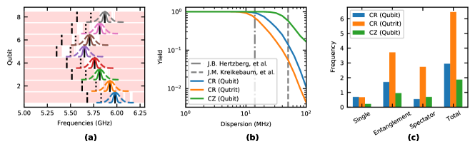
Figure 1: (a) Collision regions of an 8-qubit ring. The solid black line indicates the $\ket{0}\rightarrow\ket{1}$, the dashed black line the $\ket{1}\rightarrow\ket{2}$ transition, and the dotted line the 2-photon transitions $\ket{0}\rightarrow\ket{2}$. The red regions indicate regions considered as collisions for the device. We have plotted the normal distribution of frequency for the state-of-the-art dispersion from [16] (solid) and [17] (dashed). (b) The yield of zero-collision devices for different architectures as a function of average frequency dispersion. (c) Frequency of each category of collision for the different architectures on the 8-qubit ring. See main text for a discussion.

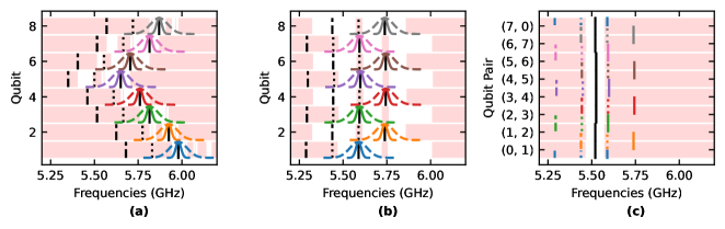
Figure S2: (a) Collision regions of an 8-qubit ring for the qubit CR architecture. The solid black line indicates the $\ket{0}\rightarrow\ket{1}$, the dashed black line the $\ket{1}\rightarrow\ket{2}$ transition, and the dotted line the 2-photon transitions $\ket{0}\rightarrow\ket{2}$. The red regions indicate regions considered as collisions for the device. We have plotted the normal distribution of the optimized frequencies for dispersions of $\sigma_{f}=15(50)$ MHz with the dashed (solid) lines. (b) Corresponding collision regions of an 8-qubit for the qubit CZ architecture. (c) Allowed regions for the CZ drive applied to each qubit in a specific qubit pair. Since the drive is no longer restricted to be exactly equal to the target qubit frequency, as it is in the CR architecture, it can be adjusted in situ within the allowed region (white) once the actual qubit frequencies (colored) are known.

To build intuition about the result of the frequency optimization, we discuss in this section the optimization of an 8-transmon ring. Such a linear topology is the minimum connectivity possible for a quantum processor and sets an upper limit on the fabrication yield one can expect. In Figure S2 we present the frequency pattern obtained with the optimization described in the preceding section, along with the allowed regions for the frequencies of each transmon. We also present the yield as a function of frequency dispersion, with the state-of-the-art fabrication dispersions with and without postprocessing denoted to give a sense of achievable yields [16, 17].

With a qubit CR-based architecture, even a linear topology with state-of-the-art dispersion of 50 MHz leads to a low yield of 10%. This yield can be increased with a postprocessing fabrication dispersion of 14 MHz, which highlights the need for techniques such as laser-annealing for further reducing the frequency dispersion. In Figure S2c we can see the distribution of errors among the different types of collisions. The majority of the collisions come from the entanglement constraints; these significantly reduce the overall yield.

In Figure S2 we also present the yield for a qutrit CR-based architecture, which has a lower yield than the corresponding qubit architecture due to the increased number of constraints. Here we optimize the frequency layout for the qubit constraints and simply calculate the yield on the qutrit architecture with the additional constraints added. Note that the frequency of single-transmon collisions remains the same for both the qubit and qutrit architectures because the optimization fixes the same anharmonicity $\alpha$ for every transmon and the energy spectrum of the transmon. This suggests that while fabricating collision-free devices using qutrit entanglement is difficult, single-qutrit gates can be implemented with few frequency collisions on a qubit-optimized device.

Finally, we also present the yield for a qubit architecture based on the differential AC-Stark shift gate. Because of the extra degree of freedom offered by the frequency of the entangling drive, the yield is much higher, and we see a larger plateau region where the yield is approximately perfect. To calculate the yield of this specific architecture, we sampled random frequencies around the target layout frequency, and for each random sample, we used the optimizer to find a new set of optimal driving frequencies for the entangling gate. For this architecture, state-of-the-art fabrication without postprocessing is already capable of reaching a high yield of 90%, and almost perfect yield can be attained with additional postprocessing. Compared with the CR-based architecture, the collision rates decrease for both single- and two-qubit gates because of the relaxation of the drive frequency constraints for entangling operations.

IV Scaling to lattices

.

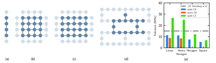
Figure 2: (a-d) Common lattice layouts. The link represents the connectivity or the possibility of realizing entanglement between its two qubits. In practice, we simulate the behavior of a unit cell with periodic boundary conditions to extract the yield. (a) A linear chain with a unit cell of 8 sites. (b) A square lattice with a unit cell of 16 sites. (c) A hexagonal lattice of 20 sites. (d) A heavy hexagon lattice with a unit cell of 15 sites. (e) Tolerance on the dispersion of the frequency to achieve a 10% yield on different lattice topologies. For the qutrit case on the hexagon and square lattices, our qubit solution was not compatible with qutrit constraints. The dashed line indicates the dispersion obtained by [17] with laser-annealing.

As the number of transmons on a processor increases, so does the number of collisions. For large systems, individually optimizing all the frequencies on a chip becomes intractable simply because of the number of variables and constraints. Instead, a smaller unit cell of frequencies must be optimized and then tiled to generate a larger lattice. To construct such a solution, we start by defining the unit cell to be tiled. To ensure that the tiling is possible, we optimize the frequency layout with periodic boundary conditions, ensuring that the solution is also valid for the larger lattice. Since calculating the yield is quick for the CR case, we can directly calculate the zero-collision yield for these large lattices. Figure 2 shows the yield for different lattices with different connectivities: a square lattice for the surface code, a heavy hexagonal lattice used by IBM [27], and a hexagonal lattice for comparison with its heavy counterpart.

When scaling to larger lattices from a given unit cell, the yield of the system can be estimated up to boundary effects with a simple scaling law,

$$y=y_{\text{m}}^{N/n_{\text{m}}}=y_{0}^{N},$$ (2)

where $y$ is the yield of the larger system, $y_{m}$ is the yield of the unit cell with periodic boundary conditions, $N$ is the total number of transmons in the system and $n_{m}$ is the number of transmons in the unit cell. Since the boundary effects will only reduce the number of potential collisions, this provides a lower bound on the yield, even for smaller system sizes. This method provides a way for comparing the scalability of different types of lattices.

In Figure 2 we show the frequency dispersion required to achieve a yield of $10\%$ for a 1,000-qubit lattice of each type. Unsurprisingly, the more densely connected lattice has a lower yield. We note that given the thresholds listed in Table 1 for a CR-based qubit architecture, none of these lattices can be fabricated with such a yield given even the best-demonstrated frequency dispersion with postprocessing. This shows that a collision-free 1,000-qubit device is likely unachievable for the CR-based architecture without a significant improvement in fabrication precision or a relaxation of the constraints. In contrast, the AC-Stark shift-based qubit architecture can scale to 1,000 qubits for two of the four lattices with a frequency dispersion already attainable with postprocessing.

V Conclusion

In this article, we have discussed the optimization of the frequency layout of fixed-frequency superconducting quantum processors. We have discussed the yield of the Cross-Resonance architecture for qubit and qutrit. We have also shown that using the differential AC-Stark shift to realize a CZ entanglement gate gives an extra degree of freedom on the entanglement drive frequency and improves the yield of this architecture, thus improving the scaling possibility of this architecture. Fixed-frequency quantum processor with transmon is currently one of the most developed architectures for multi-qubit systems, however, other qubit designs like fluxonium [23] can also realize quantum processors and will have different frequency constraints that can potentially give an advantage over transmon in terms of yield.

The submitted manuscript has been created by UChicago Argonne, LLC, Operator of Argonne National Laboratory (“Argonne”). Argonne, a U.S. Department of Energy Office of Science laboratory, is operated under Contract No. DE-AC02-06CH11357. The U.S. Government retains for itself, and others acting on its behalf, a paid-up nonexclusive, irrevocable worldwide license in said article to reproduce, prepare derivative works, distribute copies to the public, and perform publicly and display publicly, by or on behalf of the Government. The Department of Energy will provide public access to these results of federally sponsored research in accordance with the DOE Public Access Plan http://energy.gov/downloads/doe-public-access-plan.

VI Transmon model

Transmons are multilevel systems that can be approximated by a weakly anharmonic oscillator. The energy of the $n$th level is given by

$$E_{n}/h=f_{n}=nf_{0}+n(n-1)\frac{\alpha}{2},$$ (S1)

where $h$ is the Planck constant, $f_{0}$ is the frequency of the $0\mapsto 1$ transition, and $\alpha$ is the anharmonicity. In practice, $f_{0}$ is within $4.5--6$ GHz, and $\alpha$ is typically between $-200$ and $-350$ MHz. The transition frequencies are then given by

$$f_{ij}=f_{i}-f_{j}=(i-j)f_{0}+(i-j)(i+j-1)\frac{\alpha}{2}.$$ (S2)

These transition frequencies are considered when looking at collisions. The transition to avoid is the transition that goes from a state that can be populated (0 and 1 for qubits) to another state. In some situations, 2-photon transitions also have to be considered; in this case, the transition frequency is given by half the frequency of the 2-photon transition.

VII Constraints for qubit architecture

We now describe the frequency constraints and collisions on a CR architecture where the transmons are used as qubits. The constraints are listed in Table I of the main text.

.

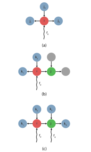
Figure S1: Configuration of the different sites considered. (a) Addressability constraint. The transmon $i$ is neighbors to $j_{1}$,$j_{2}$,$j_{2}$. When applying a pulse at the $\ket{0}\rightarrow\ket{1}$ or $\ket{1}\rightarrow\ket{2}$ transition of $i$, the frequency of the pulse must avoid the transition frequencies of these neighbors. (b) Spectators constraints for the CR architecture. (c) Spectator constraints for the CZ architecture.

VII.1 Spectators of the single-qubit gates

Manipulating a qubit, that is sending a pulse at its transition between the $0$ and the 1 state, should not drive its neighbors’ transmons transitions. Since qubits populate only the states 0 and 1, we have to avoid the 0-1 transition and the 1 to 2 transitions. This leads to two constraints that we will refer to as A constraints:

• Type A1: $f_{d}=f_{i}$. Avoid the $0\mapsto 1$ transitions of $j$:

  $$\left|f_{d}-f_{j}\right|\geq\delta_{A1}\qquad\forall(i,j)\in E$$ (S3)

• Type A2: $f_{d}=f_{i}$. Avoid the $1\mapsto 2$ transitions of $j$:

  $$\left|f_{d}-f_{j}-\alpha_{j}\right|\geq\delta_{A2}\qquad\forall(i,j)\in E$$ (S4)

To code these constraints, we notice that the constraint A1 can be applied to the directed graph $\vec{E}$, whereas because of the asymmetry in A2, we have cut the second constraint into two constraints: one as described in the equation and another with the inversion of the two indices $i$ and $j$ to be applied to the oriented edges.

VII.2 Entanglement with CR constraints

We have a constraint on the frequency difference for an interaction gate to be fast enough:

• Type C1: Gate fast enough for $f_{d}=f_{j}$:

  $$f_{i}+\alpha_{i}\leq f_{d}\leq f_{i}\qquad\forall(i,j)\in\vec{E}.$$ (S5)

For our optimization scheme, we introduce $\delta_{C1}=5$ MHz to control this constraint in the objective function:

$$f_{d}-f_{i}-\alpha_{i}\geq\delta_{C1}\qquad\forall(i,j)\in\vec{E}$$ (S6)

and

$$f_{i}-f_{d}\geq\delta_{C1}\qquad\forall(i,j)\in\vec{E}.$$ (S7)

The entanglement gate is performed with the CR interaction where a pulse at the frequency of the target transmon $j$ is applied to the control transmon $i$. One requirement for this gate to work efficiently is to not affect the control transmon, meaning that the frequency of the applied pulse has to be far enough from the various transition of the control transmon. These constraints apply to the oriented edges of the graph $\vec{E}$. There is a collision when the drive frequency $f_{d}$ collides with a transition of the control qubits. Since the drive is strong, we must also avoid the 2-photon transitions as well as the 1-photon transitions:

• Type E1: $f_{d}$ must avoid the $0\mapsto 1$ transition of $i$:

  $$\left|f_{d}-f_{i}\right|\geq\delta_{E1}\qquad\forall e=(i,j)\in\vec{E}$$ (S8)

• Type E2: $f_{d}$ must avoid the $1\mapsto 2$ transition of $i$:

  $$\left|f_{d}-f_{i}-\alpha_{i}\right|\geq\delta_{E2}\qquad\forall(i,j)\in\vec{E}$$ (S9)

• Type D1: $f_{d}$ must avoid the $0\mapsto 2$ 2-photon transitions of $i$:

  $$\left|f_{d}-f_{i}-\alpha_{i}/2\right|\geq\delta_{D1}\qquad\forall(i,j)\in\vec{E}$$ (S10)

We note that since $f_{d}=f_{j}$, the constraints E1 and E2 are included in the A1 and A2 constraints. We include them because they decrease the fidelity of different gates (single-qubit gate and entanglement gate) and the distinction will be even more relevant for the off-resonant driving used for the SiZZle gate.

VII.3 Entanglement pulses: spectators

Another constraint when performing the entanglement drive is to not influence the other neighbors’ transmons. This is related to the addressability, but in the context of entanglement gates, and is usually referred to as a spectator collision. The conditions are then identical to the addressability constraints $A_{n}$ but now with the frequency drive of the entanglement gate $f_{d}$, and the set of transmons affected is given by the set of transmons neighbors to the transmon where the drive is applied. We denote this set by $N$. For the CR gate, the pulse is applied only to the control transmon $i$ of the edge $(i,j)$, so it includes only the neighbors of $i$ that are not $j$.

$$\mathcal{N}=\{ (i,j,k)\in V^{3}:(i,j)\in\vec{E}\text{ with }(i,k)\in\vec{E}\text{ or }$$ (S11)

$$(k,i)\in\vec{E}\text{ and }j\neq k\}$$

• Type S1: $f_{d}$ must avoid the $0\mapsto 1$ transitions of $k$:

  $$\left|f_{d}-f_{k}\right|\geq\delta_{S1}\qquad\forall(i,j,k)\in\mathcal{N}$$ (S12)

• Type S2: $f_{d}$ must avoid the $1\mapsto 2$ transitions of $k$:

  $$\left|f_{d}-f_{k}-\alpha_{k}\right|\geq\delta_{S2}\qquad\forall(i,j,k)\in\mathcal{N}$$ (S13)

A more subtle type of collision can occur when the sum of the frequencies of the target and a neighbor is equal to the frequency of the $\ket{0}\rightarrow\ket{2}$ 2-photon transition. This is expressed with

• Type T1: The sum of neighbor frequencies must avoid the $\ket{0}\rightarrow\ket{2}$ transition of $k$:

  $$\left|f_{d}+f_{k}-2f_{i}-\alpha_{i}\right|\geq\delta_{T1}\qquad\forall(i,j,k)\in\mathcal{N}.$$ (S14)

VIII Constraints for CR qutrit architecture

Following [13, 14], a qutrit processor can be realized on fixed-frequency transmon architectures. Universal single-qutrit control can be realized through the use of the $\ket{0}\mapsto\ket{1}$ and the $\ket{1}\mapsto\ket{2}$ transitions. The entanglement gate can be realized with the cross-resonance interaction with these same transitions of the target transmons. Therefore, mobilizing qutrits requires adding these new drives to the constraint list. We list them in Table S1. For the addressability constraints, we split the constraints into two categories: the $\ket{0}\mapsto\ket{1}$ drive leads to the usual $A_{i}$ constraints, and the $\ket{1}\mapsto\ket{2}$ drive leads to the $B_{i}$ constraints. Note that because the state $\ket{2}$ can now be populated, the unwanted driving of the transition $\ket{2}\mapsto{3}$ transition needs to be considered. For the entanglement and spectator constraints, we have simply parametrized the drive frequency in the constraints and both drive frequencies need to be considered. We note that one possible architecture (less constrained than a full-qutrit processor) is to use the $\ket{1}\mapsto\ket{2}$ transition or single-transmon drive and use only the $f_{d}=f_{j}$ entanglement drive. This type of architecture can also be useful and removes several constraints but requires more overhead.

Table S1: Constraints imposed by the architecture on the frequency allocation on the graph for a CR qutrit architecture, following the notation of Table I. The indices refer to the participants and are defined by the graph underlying the processors. $\vec{E}$ represents the oriented graph, and $E$ represents the unoriented graph, meaning that each edge is taken into account twice, once in each direction. The frequency of the drive microwave $f_{d}$ can take two values for the qutrit case: the frequency of the target qubit $f_{d}=f_{j}$ and the frequency of the $\ket{1}\mapsto\ket{2}$ transition $f_{d}=f_{j}+\alpha_{j}$. Since there is no full analysis of the performance of the qutrit CR gate as a function of the threshold, we have used the same values for the bounds as for the qubit case.

			Definition	Participants	Bounds	Drive Frequency
Addressability	A1		$\left|f_{i}-f_{j}\right|\geq\delta_{A1}$	$(i,j)\in E$	17 MHz
	A2		$\left|f_{i}-f_{j}-\alpha_{j}\right|\geq\delta_{A2}$	$(i,j)\in E$	30 MHz
	A3		$\left|f_{i}-f_{j}-2\alpha_{j}\right|\geq\delta_{A3}$	$(i,j)\in E$	30 MHz
	B1		$\left|f_{i}+\alpha_{i}-f_{j}\right|\geq\delta_{B1}$	$(i,j)\in E$	30 MHz
	B2		$\left|f_{i}+\alpha_{i}-f_{j}-\alpha_{j}\right|\geq\delta_{B2}$	$(i,j)\in E$	17 MHz
	B3		$\left|f_{i}+\alpha_{i}-f_{j}-2\alpha_{j}\right|\geq\delta_{B3}$	$(i,j)\in E$	30 MHz
Entanglement	C1		$f_{i}+\alpha_{i}\leq f_{d}\leq f_{i}$	$(i,j)\in\vec{E}$	—
	E1		$\left|f_{d}-f_{i}\right|\geq\delta_{E1}$	$(i,j)\in\vec{E}$	17 MHz
	E2		$\left|f_{d}-f_{i}-\alpha_{i}\right|\geq\delta_{E2}$	$(i,j)\in\vec{E}$	30 MHz
	E3		$\left|f_{d}-f_{i}-2\alpha_{i}\right|\geq\delta_{E3}$	$(i,j)\in\vec{E}$	30 MHz
	D1		$\left|f_{d}-f_{i}-\alpha_{i}/2\right|\geq\delta_{D1}$	$(i,j)\in\vec{E}$	2 MHz	$f_{d}=f_{j}$
	D2		$\left|f_{d}-f_{i}-3\alpha_{i}/2\right|\geq\delta_{D2}$	$(i,j)\in\vec{E}$	2 MHz	and
Spectators	S1		$\left|f_{d}-f_{k}\right|\geq\delta_{S1}$	$(i,j,k)\in N$	17 MHz	$f_{d}=f_{j}+\alpha_{j}$
	S2		$\left|f_{d}-f_{k}-\alpha_{k}\right|\geq\delta_{S2}$	$(i,j,k)\in N$	25 MHz
	S3		$\left|f_{d}-f_{k}-2\alpha_{k}\right|\geq\delta_{S3}$	$(i,j,k)\in N$	25 MHz
	T1		$\left|f_{d}+f_{k}-2f_{i}-\alpha_{i}\right|\geq\delta_{T1}$	$(i,j,k)\in N$	17 MHz
	T2		$\left|f_{d}+f_{k}+\alpha_{k}-2f_{i}-3\alpha_{i}\right|\geq\delta_{T2}$	$(i,j,k)\in N$	17 MHz

IX Constraints for CZ qubit architecture

The differential AC-Stark shift considerably changes the constraints of the architecture: The addressability is unchanged compared with the qubit CR case, but the drive frequency of the entanglement gate can now take any frequency and is not set by the target transmon. This introduces an extra degree of freedom in the problem. We now need to find out whether there exists a drive satisfying the constraints for a given layout. This differential AC-Stark shift requires driving both qubits at the drive frequency. This leads to new constraints for the entanglement drive involving the neighbors of the second qubit, constraints that were absent from the one-qubit case. Table S2 lists the constraints we have considered.

Table S2: Constraints imposed by the architecture on the frequency allocation on the graph for a differential AC-Stark shift qubit architecture, following the notation of Table I. The indices refer to the participants and are defined by the graph underlying the processors. $\vec{E}$ represents the oriented graph, and $E$ represents the unoriented graph, meaning that each edge is taken into account twice in each direction. The frequency of the drive microwave $f_{d}$ can take any arbitrary value within the constraints. Since the AC-Stark shift is obtained by applying a drive on both qubits, we need to add the constraint with an additional “$t$” that indicates that the target’s frequency also needs to be part of the constraints. For the spectators’ errors, we need to consider the neighbors of both qubits, depicted by the ensemble $\tilde{N}$ that includes the neighbors of both $i$ and $j$. Since there is no full analysis of the performance of the AC-Stark shift gate as a function of the thresholds, we have used the same values for the bounds as for the CR qubit case.

			Definition	Participants	Bounds	Drive Frequency
Addressability	A1		$\left|f_{i}-f_{j}\right|\geq\delta_{A1}$	$(i,j)\in E$	17 MHz
	A2		$\left|f_{i}-f_{j}-\alpha_{j}\right|\geq\delta_{A2}$	$(i,j)\in E$	30 MHz
Entanglement	C1		$f_{i}+\alpha_{i}\leq f_{d}\leq f_{i}$	$(i,j)\in\vec{E}$	—
	C1t		$f_{j}+\alpha_{j}\leq f_{d}\leq f_{j}$	$(i,j)\in\vec{E}$	—
	E1		$\left|f_{d}-f_{i}\right|\geq\delta_{E1}$	$(i,j)\in\vec{E}$	17 MHz
	E2		$\left|f_{d}-f_{i}-\alpha_{i}\right|\geq\delta_{E2}$	$(i,j)\in\vec{E}$	30 MHz
	E1t		$\left|f_{d}-f_{j}\right|\geq\delta_{E1}$	$(i,j)\in\vec{E}$	17 MHz	$f_{d}$ is a free parameter
	E2t		$\left|f_{d}-f_{j}-\alpha_{j}\right|\geq\delta_{E2}$	$(i,j)\in\vec{E}$	30 MHz
	D1		$\left|f_{d}-f_{i}-\alpha_{i}/2\right|\geq\delta_{D1}$	$(i,j)\in\vec{E}$	2 MHz
	D1t		$\left|f_{d}-f_{j}-\alpha_{j}/2\right|\geq\delta_{D1}$	$(i,j)\in\vec{E}$	2 MHz
Spectators	S1		$\left|f_{d}-f_{k}\right|\geq\delta_{S1}$	$(i,j,k)\in\tilde{N}$	17 MHz
	S2		$\left|f_{d}-f_{k}-\alpha_{k}\right|\geq\delta_{S2}$	$(i,j,k)\in\tilde{N}$	25 MHz
	T1		$\left|f_{d}+f_{k}-2f_{i}-\alpha_{i}\right|\geq\delta_{T1}$	$(i,j,k)\in\tilde{N}$	17 MHz

X Optimization strategy

Finding an appropriate objective was an iterative process. Initially, we used $\delta_{i}$ to quantify the degree to which each set of constraints (on the respective frequencies and anharmonicities) is satisfied. Our first attempt was to maximize the sum of all $\delta_{i}$. For simple connectivity graphs, the MIP solution produced poor yields due to $\delta_{i}$ being zero for some $i$.

We next tried the objective

$$\operatornamewithlimits{maximize}\sum_{i}(\delta_{i}-\bar{\delta}_{i})$$ (S15)

while constraining $\delta_{i}\geq\bar{\delta}_{i}$ where $\bar{\delta}_{i}$ are the bounds declared in Tables S1 and S2. Unfortunately, this objective also resulted in some of the $\delta_{i}$ taking their lower bound value $\bar{\delta}_{i}$. We also considered weighting the terms in (S15) by counting how often each set of constraints corresponding to each $\delta_{i}$ is violated in a collision. While we tried ad-hoc increases for the weights applied to terms with more collisions, we did not find a consistent scheme for adjusting weights.

Because different terms in (S15) were zero in some solutions, we considered a second step where we introduce a new scalar variable $K$ and optimize the objective

$$\operatornamewithlimits{maximize}K$$ (S16)

subject to the additional constraints $K\leq(\delta_{i}-\bar{\delta}_{i})$ for each group of constraints $i$. This produced an optimal value $K^{*}$. We then re-solved (S15) with the additional constraints $K^{*}\leq(\delta_{i}-\bar{\delta}_{i})$ for each group of constraints $i$. This helped drive all the $\delta_{i}$ away from their lower bounds (if possible) and then allowed for an additional step of optimization.

This greatly improved the yield, so we considered a final polishing step to provide further improvement. After the above process, we set $K_{i}^{*}$ to be the difference between each $\delta_{i}$ and its lower bound. We then took this quantity and introduced additional variables $\delta_{i,e}$ for each $e\in E$ and solved

$$\operatornamewithlimits{maximize}\sum_{i}\sum_{e\in E}\delta_{i,e}$$ (S17)

subject to the constraints that $\delta_{i,e}\geq K_{i}^{*}$ from the second step.

XI Scaling

.

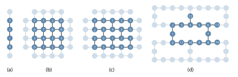
Figure S3: Site numbering for the lattice frequencies in Table S3. The unit cell for the linear chain (a) has size $n=8$.

Table S3: Optimized frequencies for the lattices shown in Figure 2 in the main text. Qubit anharmonicities were fixed to 350 MHz for every site.

Lattice	Site	CR Frequency	CZ Frequency
Linear	0	5.980	4.7385
	1	5.925	4.5935
	2	5.815	4.7435
	3	5.760	4.5985
	4	5.650	4.7435
	5	5.705	4.5935
	6	5.815	4.7385
	7	5.870	4.5885
Square	0	5.8530	4.5748
	1	5.7822	4.6296
	2	5.9486	4.7522
	3	5.7508	4.6296
	4	5.7194	4.7392
	5	5.9172	4.5748
	6	5.8844	4.7522
	7	5.8136	4.5748
	8	5.9800	4.6296
Hexagon	0	4.722	4.980
	1	4.694	4.830
	2	4.607	4.975
	3	4.733	4.830
	4	4.520	4.975
	5	4.646	4.830
Heavy Hexagon	0	4.575	4.731
	1	4.630	4.596
	2	4.520	4.731
	3	4.630	4.596
	4	4.575	4.731
	5	4.685	4.596
	6	4.630	4.731
	7	4.685	4.596
	8	4.575	4.731
	9	4.630	4.596
	10	4.520	4.731
	11	4.630	4.596
	12	4.630	4.731
	13	4.685	4.596
	14	4.630	4.596

To check how the yield scales as we increase the lattice size, we calculate the yield for a system with periodic boundaries conditions. Each unit cell is a 5x5 square lattice of qubits and we use constraints for the CR architecture. We then tile this solution to create a larger $n\times n$ system and calculate the yield. Figure S4 shows the evolution of the yield with an increasing number of sites. The linear correlation in the log-log plot shows that the yield for the large lattice can be calculated with a simple exponential law given in Eq. 2. In Figure S4 (b) we show the correlation coefficient between the yield for the periodic unit cell and the yield for the larger system, normalized by the system size. For larger systems, the correlation is almost one; for smaller systems, the correlation is lower, which indicates that boundary effects play a significant role in the yield for smaller systems. As the system size increases, these boundary effects become less important. We note this boundary effect is simply because some constraints don’t exist on the edges of the lattice, compared to the bulk. This reduces the number of constraints at the edges, and thus Eq. 2 of the main text gives an upper bound on the yield of the lattice.

.

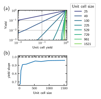
Figure S4: Scaling properties of the yield as a function of the unit cells yield with a periodic boundary condition. (a) Shows that the yield of the large system scales as a power law of the cell yield. (b) Shows the scaling compared with the unit cell for the different sizes of the system. For the small system, border effects are strong; for the large system, the ratio is close to 1, indicating small border effects.

References

- Arute et al. [2019] F. Arute, K. Arya, R. Babbush, D. Bacon, J. C. Bardin, R. Barends, R. Biswas, S. Boixo, F. G. S. L. Brandao, D. A. Buell, B. Burkett, Y. Chen, Z. Chen, B. Chiaro, R. Collins, W. Courtney, A. Dunsworth, E. Farhi, B. Foxen, A. Fowler, C. Gidney, M. Giustina, R. Graff, K. Guerin, S. Habegger, M. P. Harrigan, M. J. Hartmann, A. Ho, M. Hoffmann, T. Huang, T. S. Humble, S. V. Isakov, E. Jeffrey, Z. Jiang, D. Kafri, K. Kechedzhi, J. Kelly, P. V. Klimov, S. Knysh, A. Korotkov, F. Kostritsa, D. Landhuis, M. Lindmark, E. Lucero, D. Lyakh, S. Mandrà, J. R. McClean, M. McEwen, A. Megrant, X. Mi, K. Michielsen, M. Mohseni, J. Mutus, O. Naaman, M. Neeley, C. Neill, M. Y. Niu, E. Ostby, A. Petukhov, J. C. Platt, C. Quintana, E. G. Rieffel, P. Roushan, N. C. Rubin, D. Sank, K. J. Satzinger, V. Smelyanskiy, K. J. Sung, M. D. Trevithick, A. Vainsencher, B. Villalonga, T. White, Z. J. Yao, P. Yeh, A. Zalcman, H. Neven, and J. M. Martinis, Nature 574, 505 (2019).
- Jurcevic et al. [2021] P. Jurcevic, A. Javadi-Abhari, L. S. Bishop, I. Lauer, D. F. Bogorin, M. Brink, L. Capelluto, O. Günlük, T. Itoko, N. Kanazawa, et al., Quantum Science and Technology 6, 025020 (2021).
- Preskill [2018] J. Preskill, Quantum 2, 79 (2018).
- Campbell et al. [2017] E. T. Campbell, B. M. Terhal, and C. Vuillot, Nature 549, 172–179 (2017).
- Leek et al. [2009] P. J. Leek, S. Filipp, P. Maurer, M. Baur, R. Bianchetti, J. M. Fink, M. Göppl, L. Steffen, and A. Wallraff, Phys. Rev. B 79, 180511 (2009).
- Chow et al. [2012] J. M. Chow, J. M. Gambetta, A. D. Córcoles, S. T. Merkel, J. A. Smolin, C. Rigetti, S. Poletto, G. A. Keefe, M. B. Rothwell, J. R. Rozen, M. B. Ketchen, and M. Steffen, Phys. Rev. Lett. 109, 060501 (2012).
- Poletto et al. [2012] S. Poletto, J. M. Gambetta, S. T. Merkel, J. A. Smolin, J. M. Chow, A. D. Córcoles, G. A. Keefe, M. B. Rothwell, J. R. Rozen, D. W. Abraham, C. Rigetti, and M. Steffen, Phys. Rev. Lett. 109, 240505 (2012).
- Chow et al. [2013] J. M. Chow, J. M. Gambetta, A. W. Cross, S. T. Merkel, C. Rigetti, and M. Steffen, New J. Phys. 15, 115012 (2013).
- Cross and Gambetta [2015] A. W. Cross and J. M. Gambetta, Phys. Rev. A 91, 032325 (2015).
- Egger et al. [2019] D. Egger, M. Ganzhorn, G. Salis, A. Fuhrer, P. Müller, P. Barkoutsos, N. Moll, I. Tavernelli, and S. Filipp, Phys. Rev. Appl. 11, 014017 (2019).
- Krinner et al. [2020] S. Krinner, P. Kurpiers, B. Royer, P. Magnard, I. Tsitsilin, J.-C. Besse, A. Remm, A. Blais, and A. Wallraff, Phys. Rev. Appl. 14 (2020).
- Kim et al. [2021] Y. Kim, A. Morvan, L. B. Nguyen, R. K. Naik, C. Jünger, L. Chen, J. M. Kreikebaum, D. I. Santiago, and I. Siddiqi, High-fidelity Toffoli gate for fixed-frequency superconducting qubits (2021), arXiv:2108.10288 [quant-ph] .
- Blok et al. [2021] M. Blok, V. Ramasesh, T. Schuster, K. O’Brien, J. Kreikebaum, D. Dahlen, A. Morvan, B. Yoshida, N. Yao, and I. Siddiqi, Phys. Rev. X 11 (2021).
- Morvan et al. [2021] A. Morvan, V. V. Ramasesh, M. S. Blok, J. M. Kreikebaum, K. O’Brien, L. Chen, B. K. Mitchell, R. K. Naik, D. I. Santiago, and I. Siddiqi, Phys. Rev. Lett. 126, 210504 (2021).
- Rigetti and Devoret [2010] C. Rigetti and M. Devoret, Phys. Rev. B 81, 134507 (2010).
- Kreikebaum et al. [2020] J. Kreikebaum, K. O’Brien, A. Morvan, and I. Siddiqi, Supercond. Sci. Technol. 33, 06LT02 (2020).
- Hertzberg et al. [2021] J. B. Hertzberg, E. J. Zhang, S. Rosenblatt, E. Magesan, J. A. Smolin, J.-B. Yau, V. P. Adiga, M. Sandberg, M. Brink, J. M. Chow, et al., npj Quantum Information 7, 1 (2021).
- Fowler et al. [2012] A. G. Fowler, M. Mariantoni, J. M. Martinis, and A. N. Cleland, Physical Review A 86 (2012).
- Mitchell et al. [2021] B. K. Mitchell, R. K. Naik, A. Morvan, A. Hashim, J. M. Kreikebaum, B. Marinelli, W. Lavrijsen, K. Nowrouzi, D. I. Santiago, and I. Siddiqi, Phys. Rev. Lett. 127, 200502 (2021).
- Magesan and Gambetta [2020] E. Magesan and J. M. Gambetta, Phys. Rev. A 101, 052308 (2020).
- Tripathi et al. [2019] V. Tripathi, M. Khezri, and A. N. Korotkov, Physical Review A 100 (2019).
- Sundaresan et al. [2020] N. Sundaresan, I. Lauer, E. Pritchett, E. Magesan, P. Jurcevic, and J. M. Gambetta, PRX Quantum 1 (2020).
- Xiong et al. [2021] H. Xiong, Q. Ficheux, A. Somoroff, L. B. Nguyen, E. Dogan, D. Rosenstock, C. Wang, K. N. Nesterov, M. G. Vavilov, and V. E. Manucharyan, Arbitrary controlled-phase gate on fluxonium qubits using differential AC-Stark shifts (2021), arXiv:2103.04491 [quant-ph] .
- Wei et al. [2021] K. X. Wei, E. Magesan, I. Lauer, S. Srinivasan, D. F. Bogorin, S. Carnevale, G. A. Keefe, Y. Kim, D. Klaus, W. Landers, N. Sundaresan, C. Wang, E. J. Zhang, M. Steffen, O. E. Dial, D. C. McKay, and A. Kandala, Quantum crosstalk cancellation for fast entangling gates and improved multi-qubit performance (2021), arXiv:2106.00675 [quant-ph] .
- Gurobi Optimization, LLC [2021] Gurobi Optimization, LLC, Gurobi Optimizer Reference Manual (2021).
- Hart et al. [2011] W. E. Hart, J.-P. Watson, and D. L. Woodruff, Math. Program. Comput. 3, 219 (2011).
- Chamberland et al. [2020] C. Chamberland, G. Zhu, T. J. Yoder, J. B. Hertzberg, and A. W. Cross, Phys. Rev. X 10, 011022 (2020).