Explicit Quantum Green Function for Scattering Problems in 2-D Potential

Abstract

In this work, we present a new result which concerns the derivation of the Green function relative to the time-independent Schrodinger equation in two dimensional space. The system considered in this work is a quantum particle that have an energy E and moves in an axi- symmetrical potential. Precisely, we have assumed that the potential $V(r)$, in which the quantum particle moves, to be equal to zero inside a disk (radius b) and to be equal a positive constant $V_{0}$ in a crown of internal radius b and external radius $a(b<a)$ and equal zero out side the crown ($r>a$). We have explored the diffusion states regime for which $E>V_{0}$. We have used, to obtain the Green function, the continuity of the solution and of its rst derivative at $r=b$ and $r=a$. We have obtained the associate Green function showing the resonance energies (absence of the reflected waves) for the case $E>V_{0}$.

1 Introduction

The method of the Green function (GF) is a very powerful tool to solve almost all the problems encountered in mathematical physics, mechanics, acoustics and electromagnetism.The GF was initially defined in the distribution theory by Green itself in the electromagnetism theory gg . Thereafter, (GF) is investigated by other researchers like Neumann neu in the theory of the Newtonian potential and Helmholtz helm in the theory of acoustics. As for the ordinary differential equations, the same differential equation can have different GFs according to the initial conditions and the boundary conditions imposed on the studied problem. Before starting to expose of our problem, we must specify some references that deal questions in wide connection with our subject. The authors bc ; bc1 have considered the problem of a thin circular plate. They assume that the plate edge is elastically supported so that the boundary values are those of the radial bending moment equals zero and the strength is proportional to the function ofthe deflection on the boundary. In ku , the authors examine GF for a circular, annular and exterior circular domain.In ki ; kiku the (GF) was obtained for the elliptic domain. ad treatedhe quantum problem relative to the scatter- ing in two dimensions. In nem ; nos ; lay ; tag the authors, in approximative approach the (GF) problem was evaluated. In our work, we will interested to theproblem that consists to compute the GF relative to the Schroedinger equation in two dimensions: the Shroedinger operator is defined to be piecewise operator on three connected circular domains ($0<r<b;b<r<a;a<r<\infty$) but with specific new boundary conditions. These boundaries conditions are useful in quantum mechanics to solve the scattering problems and also the bound states. In quantum mechanics, if the potential is constant in the crown and is zero outside (or vice versa) the solution of theSchroedinger equation and the derivative of the solution are continuous on the boundary (the edge) of the crown. Specify clearly our problem: the Schrodinger equation takes different forms depending on whether it is inside the crown ($b<r<a$) or outside. This type of problem matches in quantum mechanics to the study of a particle subjected to a potential which is a positive constant inside the crown ($b<r<a$) and zero outside the crown, that is to say: $r<b$ and $r>a$. None of these cited works, and none to our knowledge, the explicit Green’s function for a piecewise continuous potential has been calculated in two dimensions for this type of problem. The physical phenomenon that we want to describe in this work is related to the resonance phenomenon in one dimension, by extending it to two dimensions. It is therefore, a question of studying the propagation of the waves associated with quantum particles (electrons for example) issued from a source that is located at the space origin, in a homogeneous two-dimensional medium. During propagation, the particles (waves) enter a coronal region (barrier) in which they are subjected to a constant potential $V_{0}$. Then they cross this region to go to infinity (r tends to infinity). Another feature of quantum particles, which is not encountered in classical mechanics, is the well-known the resonance phenomenon in the scattering regime: when a quantum particle crosses a potential barrier, with an energy $E>V_{0}$, the probability that the particle reflects is in general not zero, but it exists certain values of E (resonance energies) for which there is no reflexion, that is to say there is a total transmission.

So our paper will be organized as it follows: in the next section (Sect.2), we give a brieve overview on Green’s function and its construction, whereas in the third section we expose the problem we will solve. In section three (Sect.4), we will calculate the (GF) for the diffusion regime. It turns out that the resonance energies are obtained from the poles of the (GF) in the region $r<b$. We end our paper by a conclusion in Sect.5.

2 A brieve Green’s function overview

Suppose we have a differential equation of order $n$:

$$L\left[y\right]\equiv p_{0}\left(x\right)y^{\left(n\right)}+p_{1}\left(x\right)y^{\left(n-1\right)}+...+p_{n}\left(x\right)y=0$$ (2.1)

where the functions $p_{0}\left(x\right),p_{1}\left(x\right),...,p_{n}\left(x\right)$ are continuous on $[a,b]$, $p_{0}(x)\neq 0$ on $[a,b]$, and the boundary conditions are

$$V_{k}\left(y\right) = \alpha_{k}y\left(a\right)+\alpha_{k}^{1}y^{\prime}\left(a\right)+...+\alpha_{k}^{n-1}y^{\left(n-1\right)}+\beta_{k}y\left(b\right)+\beta_{k}^{1}y^{\prime}\left(b\right)+$$ (2.2)

$$...+\beta_{k}^{n-1}y^{\left(n-1\right)}\left(b\right),\text{ \ \ \ \ \ \ }\left(k=1,2,...,n\right)\text{\ }$$

where the linear forms $V_{1},...,V_{n}$ in $y\left(a\right),y^{\prime}\left(a\right),...,y^{\left(n-1\right)}\left(a\right),y\left(b\right),y^{\prime}\left(b\right),...,$

$y^{\left(n-1\right)}\left(b\right)$ are linearly independent.

We assume that the homogeneous boundary-value problem (2.1)-(2.2) has only a trivial solution $y(x)\equiv 0$.

Definition: Green’s function of the boundary-value problem(2.1)-(2.2) is the function $G(x,\xi)$ constructed for any point $\xi$ such that $a<\xi<b$, and having the following four properties:

(I) $G(x,\xi)$ is continuous and has continuous derivatives with respect to $x$ up to order $(n-2)$ inclusive for $a\leq x\leq b$.

(2) Its $(n-1)$th derivative with respect to $x$ at the point $x=\xi$ has a discontinuity of the first kind, the jump being equal to $\frac{1}{p_{0}\left(x\right)}$ , i.e.,

$$\frac{\partial^{n-1}G\left(x,\xi_{+}\right)}{\partial x^{n-1}}-\frac{\partial^{n-1}G\left(x,\xi_{-}\right)}{\partial x^{n-1}}=\frac{1}{p_{0}\left(x\right)}$$ (2.3)

(3) In each of the intervals $[a,\xi)$ and $(\xi,b$) the function $G(x,\xi)$, considered as a function of $x$, is a solution of equation (2.1):

$$L\left[G\right]=0$$ (2.4)

(4) $G(x,\xi)$ satisfies the boundary conditions (2.2):

$$V_{k}(G)=0,\text{ \ \ \ \ }(k=1,2,...,n)$$ (2.5)

On the exixtence and the unicity of the solution, we refer to the following theorem,
Theorem krasn : If the boundary-value problem (2.1)-( 2.2) has only the trivial solution $y(x)=0$, then the operator $L$ has one and only one Green’s function $G(x,\xi)$ (end theorem).
It is easy to convince ourselves that the four above conditions are fulfilled and the demonstration of the theorem is in krasn . Now we will apply this theorem to find the Green function for an interesting 2-D problem in quantum physics.

3 Axi-symmetric two dimensional quantum problem

Consider a quantum particle moving in a symmetrical potential (independent of the angle $\theta$) defined as (see fig.1):

$$V\left(r,\theta\right)=\left\{\begin{array}[]{c}0\quad\quad 0\leq r\leq b\\ V_{0}\quad\quad b\leq r\leq a\\ 0\quad\quad\quad\quad r\geq a\end{array}\right.$$ (3.1)

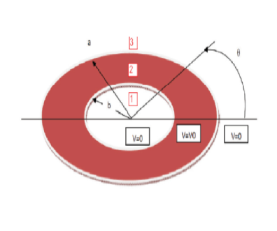
Figure 1: A scheme of the coronal potential in two dimensions

The dynamics of this particle is governed by the time-independent Schroedinger equation:

$$\hat{H}\left(r,\theta\right)\Psi(r,\theta)=E\Psi\left(r,\theta\right)$$ (3.2)

which is written in the natural polar coordinates $\left(r,\theta\right)$ and where $\hat{H}$ $\left(r,\theta\right)$ is the hamiltonien of the particle, with a mass $M$, moving in this potential. The equation (3.2) is merely an eigenvalues $E$ and eigenfuntions equation $\Psi\left(r,\theta\right)$. The explicit form of the hamiltonien of the system is:

$$\hat{H}=-\frac{\hbar^{2}}{2M}\triangle_{r,\theta}+V\left(r,\theta\right)$$ (3.3)

where:

$$\triangle_{r,\theta}=\frac{\partial^{2}}{\partial r^{2}}+\frac{1}{r}\frac{\partial}{\partial r}+\frac{1}{r^{2}}\frac{\partial^{2}}{\partial\theta^{2}}$$ (3.4)

is the well known laplacian in polar coordinates. The equation ( 3.2 ) writes as:

$$\left(-\frac{\hbar^{2}}{2M}\triangle_{r,\theta}+V\left(r,\theta\right)-E\right)\Psi\left(r,\theta\right)=0$$ (3.5)

or, with respect of the definition of $V\left(r,\theta\right)$ in the formula (3.1)

$$\left\{\begin{array}[]{c}\left(\frac{\hbar^{2}}{2M}\triangle_{r,\theta}+E\right)\Psi_{out}\left(r,\theta\right)=0\quad\quad r>a\\ \left(\frac{\hbar^{2}}{2M}\triangle_{r,\theta}-V_{0}+E\right)\Psi_{mid}\left(r,\theta\right)=0\quad\quad b\leq r\leq a\\ \left(\frac{\hbar^{2}}{2M}\triangle_{r,\theta}+E\right)\Psi_{int}\left(r,\theta\right)=0\quad\quad\quad\quad 0\leq r\leq b\end{array}\right.$$ (3.6)

This system is subjected to the boundary conditions defined as $\Psi\left(r,\theta\right)$ and $\frac{d}{dr}\Psi\left(r,\theta\right)$ are to be continous at $r=b$ and $\ r=a$ for all values of the azimutal angle $\theta$. The separation variables method leads to transform the last equations (3.6) as

$$\left\{\begin{array}[]{c}\frac{d}{dr}\left(r\frac{d}{dr}\Psi_{out}\right)+\left(\frac{2M}{\hbar^{2}}Er-\frac{l^{2}}{r}\right)\Psi_{out}(r)=0\quad\quad r>a\\ \frac{d}{dr}\left(r\frac{d}{dr}\Psi_{mid}\right)+\left(\frac{2M}{\hbar^{2}}(E-V_{0})r-\frac{l^{2}}{r}\right)\Psi_{mid}(r)=0\quad\quad b\leq r\leq a\\ \frac{d}{dr}\left(r\frac{d}{dr}\Psi_{int}\right)+\left(\frac{2M}{\hbar^{2}}Er-\frac{l^{2}}{r}\right)\Psi_{int}(r)=0\quad\quad\quad\quad 0\leq r\leq b\end{array}\right.$$ (3.7)

whose solutions are combination of two linear independent Bessel’s functions of order $l$ ($l\in Z$). The solution must obey to the boundary conditions at $r=b$ and $r=a$:

$$\Psi_{out}(a) =\Psi_{mid}(a)$$ (3.8)

$$(\frac{d\Psi_{out}(r)}{dr})_{r=a} =(\frac{d\Psi_{mid}(r)}{dr})_{r=a}$$ (3.9)

and

$$\Psi_{mid}(b) =\Psi_{int}(b)$$ (3.10)

$$(\frac{d\Psi_{mid}(r)}{dr})_{r=b} =(\frac{d\Psi_{int}(r)}{dr})_{r=b}$$ (3.11)

where $l=...-2,-1,0,+1,+2,...$. The global (GF) of the problem (3.7) augmented by the boundary conditions (8-11) is given by

$$G(\overrightarrow{r},\overrightarrow{r}^{\prime},E)=G(r,\theta,r^{\prime},\theta^{\prime},E)={\sum\limits_{l=-\infty}^{+\infty}}G(l;r,r^{\prime},E)\exp(il(\theta-\theta^{\prime}))$$

where $G(l;r,r^{\prime},E)\equiv$ $G(l;r,r^{\prime})$ is the radial (GF) that we shall calculate in the subsequent sections. To calculate the (GF) we will study separately two cases of the energy: the first case is $E>V_{0}$, which corresponds to the diffusion regime and the second is $0<E<V_{0}$ for which corresponds the bounded states regime.

4 The diffusion states regime: $E>V_{0}$

4.1 The region: $a\leq r\leq r^{\prime}<\infty$

Using the first equation of (3.7), in third region ($r>a$), the corresponding radial (GF) can be written as the following

$$G_{out}\left(l;r,r^{\prime}\right)=G^{3,3}\left(l;r,r^{\prime}\right)=\left\{\begin{array}[]{c}C\left(r^{\prime}\right)\left[Y_{l}\left(kr\right)-\beta(r^{\prime})J_{l}\left(kr\right)\right]\quad a\leq r\leq r^{\prime}\\ D\left(r^{\prime}\right)J_{l}\left(kr\right)\quad\quad r^{\prime}\leq r<\infty\end{array}\right.$$ (4.1)

where: $k^{2}=\frac{2M}{\hbar^{2}}E$. Using the continuity of the (GF) at $r=r^{\prime}$

$$G^{3,3}\left(l;r_{+}^{\prime},r^{\prime}\right)-G^{3,3}\left(l;r_{-}^{\prime},r^{\prime}\right)=0$$

then

$$\left[D\left(r^{\prime}\right)+\beta(r^{\prime})C\left(r^{\prime}\right)\right]J_{l}\left(kr^{\prime}\right)-C\left(r^{\prime}\right)Y_{l}\left(kr^{\prime}\right)=0$$ (4.2)

and the dicontinuity of the first derivative with respect $r$ at $r=r^{\prime}$:

$$\frac{d}{dr}G^{3,3}\left(l;r_{+}^{\prime},r^{\prime}\right)-\frac{d}{dr}G^{3,3}\left(l;r_{-}^{\prime},r^{\prime}\right)=\frac{2}{\pi r^{\prime}}$$

then

$$\left[D\left(r^{\prime}\right)+\beta(r^{\prime})C\left(r^{\prime}\right)\right]J_{l}^{\prime}\left(kr^{\prime}\right)-C\left(r^{\prime}\right)Y_{l}^{\prime}\left(kr^{\prime}\right)=\frac{2}{\pi kr^{\prime}}.$$ (4.3)

By comparinng ( 4.2 ) and (4.3) we check that

$$C\left(r^{\prime}\right)\left[Y_{l}\left(kr^{\prime}\right)J_{l}^{\prime}\left(kr^{\prime}\right)-J_{l}\left(kr^{\prime}\right)Y_{l}^{\prime}\left(kr^{\prime}\right)\right]=\frac{2J_{l}\left(kr^{\prime}\right)}{\pi kr^{\prime}}$$ (4.4)

and by using the Bessel Wronskian for the pair $\left(J_{l},Y_{l}\right)$:

$$W\left(J_{l}\left(kr^{\prime}\right),Y_{l}\left(kr^{\prime}\right)\right)=J_{l}\left(kr^{\prime}\right)Y_{l}^{\prime}\left(kr^{\prime}\right)-J_{l}^{\prime}\left(kr^{\prime}\right)Y_{l}\left(kr^{\prime}\right)=\frac{2}{\pi kr^{\prime}}$$ (4.5)

it is easy to get:

$$C\left(r^{\prime}\right)=-J_{l}\left(kr^{\prime}\right)$$ (4.6)

and then from (4.3) we obtain:

$$D\left(r^{\prime}\right)=\beta(r^{\prime})J_{l}\left(kr^{\prime}\right)-Y_{l}\left(kr^{\prime}\right).$$ (4.7)

After substitution of ( 4.7 ) and ( 4.6 ) in ( 4.1 ) we find the (GF) in the region ( $r,r^{\prime}\geq a$):

$$G^{3,3}\left(l;r,r^{\prime}\right)=-\left\{\begin{array}[]{c}J_{l}\left(kr^{\prime}\right)\left[Y_{l}\left(kr\right)-\beta(r^{\prime})J_{l}\left(kr\right)\right]\quad\quad a\leq r\leq r^{\prime}\\ \left[Y_{l}\left(kr^{\prime}\right)-\beta(r^{\prime})J_{l}\left(kr^{\prime}\right)\right]J_{l}\left(kr\right)\quad\quad r^{\prime}\leq r<\infty\end{array}\right..$$ (4.8)

It remains to determine the coefficient $\beta(r^{\prime})$. To do this, we use the symmetry property

$$G^{3,3}(l:r,r^{\prime})=G^{3,3}(l:r^{\prime},r)$$

then

$$\left[Y_{l}\left(kr^{\prime}\right)-\beta(r^{\prime})J_{l}\left(kr^{\prime}\right)\right]J_{l}\left(kr\right)=\left[Y_{l}\left(kr\right)-\beta(r)J_{l}\left(kr\right)\right]J_{l}\left(kr^{\prime}\right)$$

By identifying in the last equation we find

$$\beta(r^{\prime})=\beta(r)=\beta$$ (4.9)

Then the (GF) in this region ( $r,r^{\prime}\geq a$) is given by:

$$G^{3,3}\left(l;r,r^{\prime}\right)=-\left\{\begin{array}[]{c}J_{l}\left(kr^{\prime}\right)\left[Y_{l}\left(kr\right)-\beta J_{l}\left(kr\right)\right]\quad\quad a\leq r\leq r^{\prime}\\ \left[Y_{l}\left(kr^{\prime}\right)-\beta J_{l}\left(kr^{\prime}\right)\right]J_{l}\left(kr\right)\quad\quad r^{\prime}\leq r<\infty\end{array}\right.$$ (4.10)

where $\beta$ is a constant to be determined lates.

4.2 The region: $b\leq r\leq r^{\prime}\leq a$
 

The Green’s function in this region can be written as:

$$G_{mid}(l;r,r^{\prime})=G^{2,2}\left(l;r,r^{\prime}\right)=\left\{\begin{array}[]{c}E\left(r^{\prime}\right)\left[Y_{l}\left(\mu r\right)-\delta(r^{\prime})J_{l}\left(\mu r\right)\right]\quad\quad b\leq r\leq r^{\prime}\\ F\left(r^{\prime}\right)\left[Y_{l}\left(\mu r\right)-\gamma\left(r^{\prime}\right)J_{l}\left(\mu r\right)\right]\quad\quad r^{\prime}\leq r<a\end{array}\right.$$

where: $\mu^{2}=\frac{2M}{\hbar^{2}}(E-V_{0})$. To calculate the coefficients $E\left(r^{\prime}\right)$, $F\left(r^{\prime}\right)$, $\gamma(r^{\prime})$ and $\delta(r^{\prime})$ we use the continuity of the (GF) at $r=r^{\prime}$:

$$G^{2,2}\left(l;r_{+}^{\prime},r^{\prime}\right)=G^{2,2}\left(l;r_{-}^{\prime},r^{\prime}\right)$$

then

$$Y_{l}\left(\mu r^{\prime}\right)\left[F\left(r^{\prime}\right)-E\left(r^{\prime}\right)\right]-J_{l}\left(\mu r^{\prime}\right)\left[\gamma\left(r^{\prime}\right)F\left(r^{\prime}\right)-\delta(r^{\prime})E\left(r^{\prime}\right)\right]=0$$ (4.11)

and we use the discontinuity of the first derivative with respect $r$  at $r=r^{\prime}$:

$$\frac{d}{dr}G^{2,2}\left(l;r=r_{+}^{\prime},r^{\prime}\right)-\frac{d}{dr}G^{2,2}\left(l;r=r_{-}^{\prime},r^{\prime}\right)=\frac{2}{\pi r^{\prime}}$$

then

$$Y_{l}^{\prime}\left(\mu r^{\prime}\right)\left[F\left(r^{\prime}\right)-E\left(r^{\prime}\right)\right]-J_{l}^{\prime}\left(\mu r^{\prime}\right)\left[\gamma\left(r^{\prime}\right)F\left(r^{\prime}\right)-\delta(r^{\prime})E\left(r^{\prime}\right)\right]=\frac{2}{\pi\mu r^{\prime}}.$$ (4.12)

By combining ( 4.11 ) and ( 4.12 ), we obtain:

$$F\left(r^{\prime}\right)=\frac{E\left(r^{\prime}\right)\left[Y_{l}\left(\mu r^{\prime}\right)-\delta\left(r^{\prime}\right)J_{l}\left(\mu r^{\prime}\right)\right]}{\left[Y_{l}\left(\mu r^{\prime}\right)-\gamma\left(r^{\prime}\right)J_{l}\left(\mu r^{\prime}\right)\right]}$$

and

$$Y_{l}^{\prime}\left(\mu r^{\prime}\right)\left[\frac{E\left(r^{\prime}\right)\left[Y_{l}\left(\mu r^{\prime}\right)-\delta\left(r^{\prime}\right)J_{l}\left(\mu r^{\prime}\right)\right]}{\left[Y_{l}\left(\mu r^{\prime}\right)-\gamma\left(r^{\prime}\right)J_{l}\left(\mu r^{\prime}\right)\right]}-E\left(r^{\prime}\right)\right]$$

$$-J_{l}^{\prime}\left(\mu r^{\prime}\right)\left[\gamma\left(r^{\prime}\right)\frac{E\left(r^{\prime}\right)\left[Y_{l}\left(\mu r^{\prime}\right)-\delta\left(r^{\prime}\right)J_{l}\left(\mu r^{\prime}\right)\right]}{\left[Y_{l}\left(\mu r^{\prime}\right)-\gamma\left(r^{\prime}\right)J_{l}\left(\mu r^{\prime}\right)\right]}-\delta(r^{\prime})E\left(r^{\prime}\right)\right]=\frac{2}{\pi\mu r^{\prime}}$$

Using the Bessel Wronksian for the pair $\left(J_{l},Y_{l}\right)$:

$$W\left(J_{l}\left(\mu r^{\prime}\right),Y_{l}\left(\mu r^{\prime}\right)\right)=J_{l}\left(\mu r^{\prime}\right)Y_{l}^{\prime}\left(\mu r^{\prime}\right)-Y_{l}\left(\mu r^{\prime}\right)J_{l}^{\prime}\left(\mu r^{\prime}\right)=\frac{2}{\pi\mu r^{\prime}}$$ (4.13)

we get the coefficients:

$$E\left(r^{\prime}\right)=\frac{Y_{l}\left(\mu r^{\prime}\right)-\gamma\left(r^{\prime}\right)J_{l}\left(\mu r^{\prime}\right)}{g(r^{\prime})}$$ (4.14)

where

$$g(x)=\gamma\left(x\right)-\delta\left(x\right)$$ (4.15)

and

$$F\left(r^{\prime}\right)=\frac{Y_{l}\left(\mu r^{\prime}\right)-\delta\left(r^{\prime}\right)J_{l}\left(\mu r^{\prime}\right)}{g(r^{\prime})}$$ (4.16)

Then, the (GF) in the region $b\leq r\leq r^{\prime}\leq a$ is given by:
$G^{2,2}\left(l;r,r^{\prime}\right)=\frac{1}{g(r^{\prime})}\left\{\begin{array}[]{c}\left[Y_{l}\left(\mu r^{\prime}\right)-\gamma\left(r^{\prime}\right)J_{l}\left(\mu r^{\prime}\right)\right]\left[Y_{l}\left(\mu r\right)-\delta(r^{\prime})J_{l}\left(\mu r\right)\right]\\ \left[Y_{l}\left(\mu r^{\prime}\right)-\delta\left(r^{\prime}\right)J_{l}\left(\mu r^{\prime}\right)\right]\left[Y_{l}\left(\mu r\right)-\gamma\left(r^{\prime}\right)J_{l}\left(\mu r\right)\right]\end{array}\right.$

for $b\leq r\leq r^{\prime}\leq a$ and $b\leq r^{\prime}\leq r\leq a$ respectively. It remains to determine the coefficients $\delta(r^{\prime}),$ $\gamma(r^{\prime})$ and $g(r^{\prime})$. To do this, we use the symmetry property of $G(l;r,r^{\prime})$

$$G^{2,2}(l;r,r^{\prime})=G^{2,2}(l;r^{\prime},r)$$

then

$$\frac{1}{g(r^{\prime})}\left\{\begin{array}[]{c}\left[Y_{l}\left(\mu r^{\prime}\right)-\gamma\left(r^{\prime}\right)J_{l}\left(\mu r^{\prime}\right)\right]\left[Y_{l}\left(\mu r\right)-\delta(r^{\prime})J_{l}\left(\mu r\right)\right]\\ \left[Y_{l}\left(\mu r^{\prime}\right)-\delta\left(r^{\prime}\right)J_{l}\left(\mu r^{\prime}\right)\right]\left[Y_{l}\left(\mu r\right)-\gamma\left(r^{\prime}\right)J_{l}\left(\mu r\right)\right]\end{array}\right.$$

$$=\frac{1}{g(r)}\left\{\begin{array}[]{c}\left[Y_{l}\left(\mu r\right)-\gamma\left(r\right)J_{l}\left(\mu r\right)\right]\left[Y_{l}\left(\mu r^{\prime}\right)-\delta(r)J_{l}\left(\mu r^{\prime}\right)\right]\\ \left[Y_{l}\left(\mu r\right)-\delta\left(r\right)J_{l}\left(\mu r\right)\right]\left[Y_{l}\left(\mu r^{\prime}\right)-\gamma\left(r\right)J_{l}\left(\mu r^{\prime}\right)\right]\end{array}\right.$$

By identifying in the last equation we find

$$\delta\left(r\right) =\delta\left(r^{\prime}\right)=\delta=constant$$ (4.17)

$$\gamma\left(r\right) =\gamma\left(r^{\prime}\right)=\gamma=constant$$

$$g\left(r\right) =g\left(r^{\prime}\right)=g=constant$$ (4.18)

These constants we must to determine later.

4.3 The coefficients $\gamma$ and $\delta$ determination

To find the coefficients $\gamma$ and $\delta$ we use the continuity of the (GF) and the continuity of its derivative at $r=a$:

$$G^{3,3}\left(l;r,a\right)=G^{2,2}\left(l;r,a\right)$$

then

$$\frac{1}{g}\left[Y_{l}\left(\mu a\right)-\gamma J_{l}\left(\mu a\right)\right]\left[Y_{l}\left(\mu a\right)-\delta J_{l}\left(\mu a\right)\right]=-J_{l}\left(ka\right)\left[Y_{l}\left(ka\right)-\beta J_{l}\left(ka\right)\right]$$ (4.19)

and

$$\frac{d}{dr}G^{3,3}\left(l;r,a\right)\rfloor_{r=a}=\frac{d}{dr}G^{2,2}\left(l;r,a\right)\rfloor_{r=a}$$

then

$$\frac{\mu}{g}\left[Y_{l}^{\prime}\left(\mu a\right)-\gamma J_{l}^{\prime}\left(\mu a\right)\right]\left[Y_{l}\left(\mu a\right)-\delta J_{l}\left(\mu a\right)\right]=kJ_{l}\left(ka\right)\left[\beta J_{l}^{\prime}\left(ka\right)-Y_{l}^{\prime}\left(ka\right)\right]$$ (4.20)

By dividing (4.20) by (4.19) and after simplifications we get the following equation

$$\frac{\mu\left[Y_{l}^{\prime}\left(\mu a\right)-\gamma J_{l}^{\prime}\left(\mu a\right)\right]}{\left[Y_{l}\left(\mu a\right)-\gamma J_{l}\left(\mu a\right)\right]}=\frac{k\left[Y_{l}^{\prime}\left(ka\right)-\beta J_{l}^{\prime}\left(ka\right)\right]}{\left[Y_{l}\left(ka\right)-\beta J_{l}\left(ka\right)\right]}$$

from which we get the coefficient $\gamma$

$$\gamma =\frac{kY_{l}\left(\mu a\right)\left[Y_{l}^{\prime}\left(ka\right)-\beta J_{l}^{\prime}\left(ka\right)\right]-\mu Y_{l}^{\prime}\left(\mu a\right)\left[Y_{l}\left(ka\right)-\beta J_{l}\left(ka\right)\right]}{kJ_{l}\left(\mu a\right)\left[Y_{l}^{\prime}\left(ka\right)-\beta J_{l}^{\prime}\left(ka\right)\right]-\mu J_{l}^{\prime}\left(\mu a\right)\left[Y_{l}\left(ka\right)-\beta J_{l}\left(ka\right)\right]}$$ (4.21)

$$or$$

$$\gamma(k,\mu,a,b)=\frac{V(k,\mu,a,b)}{U(k,\mu,a,b)}$$ (4.22)

such that

$$V(k,\mu,\beta,a,b) =kY_{l}\left(\mu a\right)\left[Y_{l}^{\prime}\left(ka\right)-\beta J_{l}^{\prime}\left(ka\right)\right]$$

$$-\mu Y_{l}^{\prime}\left(\mu a\right)\left[Y_{l}\left(ka\right)-\beta J_{l}\left(ka\right)\right]$$ (4.23)

$$U(k,\mu,\beta,a,b) =kJ_{l}\left(\mu a\right)\left[Y_{l}^{\prime}\left(ka\right)-\beta J_{l}^{\prime}\left(ka\right)\right]$$

$$-\mu J_{l}^{\prime}\left(\mu a\right)\left[Y_{l}\left(ka\right)-\beta J_{l}\left(ka\right)\right].$$ (4.24)

By combining ( 4.19 ) and ( 4.22 ) we obtain:

$$\delta=\frac{\mu Y_{l}\left(\mu a\right)\left[Y_{l}^{\prime}\left(\mu a\right)-\gamma J_{l}^{\prime}\left(\mu a\right)\right]+k\gamma J_{l}\left(ka\right)\left[Y_{l}^{\prime}\left(ka\right)-\beta J_{l}^{\prime}\left(ka\right)\right]}{\mu J_{l}\left(\mu a\right)\left[Y_{l}^{\prime}\left(\mu a\right)-\gamma J_{l}^{\prime}\left(\mu a\right)\right]+kJ_{l}\left(ka\right)\left[Y_{l}^{\prime}\left(ka\right)-\beta J_{l}^{\prime}\left(ka\right)\right]}$$

$$\delta\equiv\delta(k,\mu,a,b)=\frac{2Y_{l}\left(\mu a\right)+\pi aJ_{l}\left(ka\right)V(k,\mu,a)}{2J_{l}\left(\mu a\right)+\pi aJ_{l}\left(ka\right)U(k,\mu,a)}.$$

Then

$$g\equiv g(k,\mu,a,b)=\gamma(k,\mu,a,b)-\delta(k,\mu,a,b)$$

but $g$ still depends on $\beta$ via the above expressions of $\gamma$ and $\delta$ themselves via V and U. We will show later that this dependence will be removed by showing that $\beta$ also depends on $k,\mu,a$ and $b.$ With the same way, we find finally, the (GF) (31) in the region $\left(b\leq r\leq a\right)$

$$G^{2,2}\left(l;r,r^{\prime}\right)=\left\{\begin{array}[]{c}\left[\frac{Y_{l}\left(\mu r^{\prime}\right)}{g(k,\mu,a,b)}-\frac{V(k,\mu,a,b)}{U(k,\mu,a,b)}\frac{J_{l}\left(\mu r^{\prime}\right)}{g(k,\mu,a)}\right]\times\\ \left[Y_{l}\left(\mu r\right)-\frac{2Y_{l}\left(\mu a\right)+\pi aJ_{l}\left(ka\right)V(k,\mu,a,b)}{2J_{l}\left(\mu a\right)+\pi aJ_{l}\left(ka\right)U(k,\mu,a,b)}J_{l}\left(\mu r\right)\right]\\ r\longleftrightarrow r^{\prime}\end{array}\right.$$

for $b\leq r\leq r^{\prime}\leq a$ and $a\leq r^{\prime}\leq r\leq a$ respectively.

4.4 The region: $0\leq r\leq r^{\prime}\leq b$

In this region, the (GF) can be written as:

$$G_{in}\left(l;r,r^{\prime}\right)\equiv G^{1,1}\left(l;r,r^{\prime}\right)=\left\{\begin{array}[]{c}A\left(r^{\prime}\right)J_{l}\left(kr\right)\quad\quad\quad 0<r\leq r^{\prime}\\ B\left(r^{\prime}\right)\left[Y_{l}\left(kr\right)-\alpha(r^{\prime})J_{l}\left(kr\right)\right]\quad r^{\prime}\leq r\leq b\end{array}\right.$$ (4.25)

where $k^{2}=\frac{2M}{\hbar^{2}}E$. To calculate the coefficients $A\left(r^{\prime}\right)$, $B\left(r^{\prime}\right)$ and $\alpha(r^{\prime})$, we use the continuity of the (GF) at $r=r^{\prime}$:

$$G^{1,1}\left(l;r_{+}^{\prime},r^{\prime}\right)-G^{1,1}\left(l;r_{-}^{\prime},r^{\prime}\right)=0$$

then

$$B\left(r^{\prime}\right)Y_{l}\left(kr^{\prime}\right)-\left[A\left(r^{\prime}\right)+\alpha(r^{\prime})B\left(r^{\prime}\right)\right]J_{l}\left(kr^{\prime}\right)=0$$ (4.26)

and we use the discontinuity of the first derivative with respect $r$ at $r=r^{\prime}$

$$\frac{d}{dr}G^{1,1}\left(l;r_{+}^{\prime},r^{\prime}\right)-\frac{d}{dr}G^{1,1}\left(l;r_{-}^{\prime},r^{\prime}\right)=\frac{2}{\pi r^{\prime}}$$

then

$$B\left(r^{\prime}\right)Y_{l}^{\prime}\left(kr^{\prime}\right)-\left[A\left(r^{\prime}\right)+\alpha(r^{\prime})B\left(r^{\prime}\right)\right]J_{l}^{\prime}\left(kr^{\prime}\right)=\frac{2}{\pi kr^{\prime}}$$ (4.27)

By combining ( LABEL:a111 ) and ( 4.36 ) we obtain

$$A\left(r^{\prime}\right)=\frac{B\left(r^{\prime}\right)\left[Y_{l}\left(kr^{\prime}\right)-\alpha(r^{\prime})J_{l}\left(kr^{\prime}\right)\right]}{J_{l}\left(kr^{\prime}\right)}$$ (4.28)

and

$$B\left(r^{\prime}\right)Y_{l}^{\prime}\left(kr^{\prime}\right)-\left[\frac{B\left(r^{\prime}\right)\left[Y_{l}\left(kr^{\prime}\right)-\alpha(r^{\prime})J_{l}\left(kr^{\prime}\right)\right]}{J_{l}\left(kr^{\prime}\right)}+\alpha(r^{\prime})B\left(r^{\prime}\right)\right]J_{l}^{\prime}\left(kr^{\prime}\right)=\frac{2}{\pi kr^{\prime}}$$ (4.29)

By using the Bessel Wronksian for the pair $\left(J_{l},Y_{l}\right)$

$$W\left(J_{l}\left(kr^{\prime}\right),Y_{l}\left(kr^{\prime}\right)\right)=J_{l}\left(kr^{\prime}\right)Y_{l}^{\prime}\left(kr^{\prime}\right)-Y_{l}\left(kr^{\prime}\right)J_{l}^{\prime}\left(kr^{\prime}\right)=\frac{2}{\pi kr^{\prime}}$$ (4.30)

we get the coefficients

$$B\left(r^{\prime}\right)=J_{l}\left(kr^{\prime}\right)$$ (4.31)

and

$$A\left(r^{\prime}\right)=\left[Y_{l}\left(kr^{\prime}\right)-\alpha(r^{\prime})J_{l}\left(kr^{\prime}\right)\right]$$ (4.32)

Then, the (GF) in this region $\left(r\leq b\right)$ is given by:

$$G^{1,1}\left(l;r,r^{\prime}\right)=\left\{\begin{array}[]{c}\left[Y_{l}\left(kr^{\prime}\right)-\alpha(r^{\prime})J_{l}\left(kr^{\prime}\right)\right]J_{l}\left(kr\right)\qquad 0<r\leq r^{\prime}\\ \left[Y_{l}\left(kr\right)-\alpha(r^{\prime})J_{l}\left(kr\right)\right]J_{l}\left(kr^{\prime}\right)\qquad r^{\prime}\leq r\leq b\end{array}\right.$$ (4.33)

It remains to determine the coefficient $\alpha(r^{\prime})$. To do this, we use the symmetry property of $G(l:r,r^{\prime})$

$$G^{1,1}(l;r,r^{\prime})=G^{1,1}(l;r^{\prime},r)$$

$$\left[Y_{l}\left(kr^{\prime}\right)-\alpha(r^{\prime})J_{l}\left(kr^{\prime}\right)\right]J_{l}\left(kr\right)=\left[Y_{l}\left(kr\right)-\alpha(r)J_{l}\left(kr\right)\right]J_{l}\left(kr^{\prime}\right)$$

By identifying in the last equation we find

$$\alpha(r^{\prime})=\alpha(r)=\alpha$$ (4.34)

Then the (GF) in this region$\left(r\leq b\right)$ is given by:

$$G^{1,1}\left(l;r,r^{\prime}\right)=\left\{\begin{array}[]{c}\left[Y_{l}\left(kr^{\prime}\right)-\alpha J_{l}\left(kr^{\prime}\right)\right]J_{l}\left(kr\right)\qquad 0<r\leq r^{\prime}\\ \left[Y_{l}\left(kr\right)-\alpha J_{l}\left(kr\right)\right]J_{l}\left(kr^{\prime}\right)\qquad r^{\prime}\leq r\leq b\end{array}\right.$$ (4.35)

We mention here that the coefficient $\alpha$ will be determined in the next subsection.

4.5
The coefficient $\alpha$ determination

To find the coefficient $\alpha$, we use the continuity of the (GF) and the continuity of its derivative at $r=b$ :

$$G^{1,1}\left(l;r,b\right)=G^{2,2}\left(l;r,b\right)$$

then

$$\left[Y_{l}\left(\mu b\right)-\frac{2Y_{l}\left(\mu a\right)+\pi aJ_{l}\left(ka\right)V(k,\mu,a,b)}{2J_{l}\left(\mu a\right)+\pi aJ_{l}\left(ka\right)U(k,\mu,a,b)}J_{l}\left(\mu b\right)\right]\times$$

$$\left[\frac{Y_{l}\left(\mu b\right)}{g(k,\mu,a,b)}-\frac{V(k,\mu,a,b)}{U(k,\mu,a,b)}\frac{J_{l}\left(\mu b\right)}{g(k,\mu,a,b)}\right]=[\alpha J_{l}(kb)-Y_{l}(kb)]J_{l}\left(kb\right)$$ (4.36)

and using

$$\frac{d}{dr}G^{1,1}\left(l;r,b\right)\rfloor_{r=b}=\frac{d}{dr}G^{2,2}\left(l;r,b\right)\rfloor_{r=b}$$

or equivalently

$$\left[Y_{l}^{\prime}\left(\mu b\right)-\frac{2Y_{l}\left(\mu a\right)+\pi aJ_{l}\left(ka\right)V(k,\mu,a,b)}{2J_{l}\left(\mu a\right)+\pi aJ_{l}\left(ka\right)U(k,\mu,a,b)}J_{l}^{\prime}\left(\mu b\right)\right]\times$$

$$\frac{\mu}{g(k,\mu,a,b)}\left[Y_{l}\left(\mu b\right)-\gamma J_{l}\left(\mu b\right)\right]=-k\left[Y_{l}\left(kb\right)-\alpha J_{l}\left(kb\right)\right]J_{l}^{\prime}\left(kb\right)$$ (4.37)

By deviding (4.37) by (4.36) we find

$$\frac{\mu\left[Y_{l}^{\prime}\left(\mu b\right)-\frac{2Y_{l}\left(\mu a\right)+\pi aJ_{l}\left(ka\right)V(k,\mu,a,b)}{2J_{l}\left(\mu a\right)+\pi aJ_{l}\left(ka\right)U(k,\mu,a,b)}J_{l}^{\prime}\left(\mu b\right)\right]}{\left[Y_{l}\left(\mu b\right)-\frac{2Y_{l}\left(\mu a\right)+\pi aJ_{l}\left(ka\right)V(k,\mu,a,b)}{2J_{l}\left(\mu a\right)+\pi aJ_{l}\left(ka\right)U(k,\mu,a,b)}J_{l}\left(\mu b\right)\right]}=\frac{kJ_{l}^{\prime}\left(kb\right)}{J_{l}\left(kb\right)}$$ (4.38)

After replacing $U$ and $V$ in (4.38) by their expressions (4.23) et (4.24) we find

$$\beta(k,\mu,a,b)=\frac{F(k,\mu,a,b)}{T(k,\mu,a,b)}$$ (4.39)

such that

$$F(k,\mu,a,b)=\mu J_{l}\left(kb\right)\left[2+k\pi aJ_{l}\left(ka\right)Y_{l}^{\prime}\left(ka\right)\right]F_{1}(k,\mu,a,b)+$$

$$kJ_{l}^{\prime}\left(kb\right)\left[2+k\pi aJ_{l}\left(ka\right)J_{l}^{\prime}\left(ka\right)\right]T_{1}(k,\mu,a,b)+$$

$$\mu\pi aJ_{l}\left(ka\right)Y_{l}\left(ka\right)\left[\mu J_{l}\left(kb\right)T_{2}(k,\mu,a,b)+kJ_{l}^{\prime}\left(kb\right)F_{2}(k,\mu,a,b)\right]$$ (4.40)

and

$$T(k,\mu,a,b)=\pi ak\mu J_{l}\left(ka\right)\times$$

$$\left[J_{l}^{\prime}\left(ka\right)J_{l}\left(kb\right)F_{1}(k,\mu,a,b)-J_{l}\left(ka\right)J_{l}^{\prime}\left(kb\right)F_{2}(k,\mu,a,b)\right]$$

$$-\pi aJ_{l}\left(ka\right)\left[\mu^{2}J_{l}\left(ka\right)J_{l}\left(kb\right)T_{2}(k,\mu,a,b)+k^{2}J_{l}^{\prime}\left(ka\right)J_{l}^{\prime}\left(kb\right)T_{1}(k,\mu,a,b)\right]$$ (4.41)

where

$$F_{1}(k,\mu,a,b)=J_{l}\left(\mu a\right)Y_{l}^{\prime}\left(\mu b\right)-Y_{l}\left(\mu a\right)J_{l}^{\prime}\left(\mu b\right)$$ (4.42)

$$F_{2}(k,\mu,a,b)=J_{l}\left(\mu b\right)Y_{l}^{\prime}\left(\mu a\right)-Y_{l}\left(\mu b\right)J_{l}^{\prime}\left(\mu a\right)$$ (4.43)

$$T_{1}(k,\mu,a,b)=J_{l}\left(\mu a\right)Y_{l}\left(\mu b\right)-Y_{l}\left(\mu a\right)J_{l}\left(\mu b\right)$$ (4.44)

$$T_{2}(k,\mu,a,b)=J_{l}^{\prime}\left(\mu b\right)Y_{l}^{\prime}\left(\mu a\right)-Y_{l}^{\prime}\left(\mu b\right)J_{l}^{\prime}\left(\mu a\right)$$ (4.45)

By using 4.26 and 4.26 and after a minor simplifications we get the coefficient $\alpha$ equal to

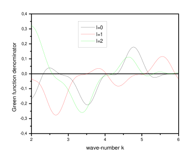
Figure 2: The resonance energies are given by the intersection of the curve with k axis for various angular momenta l=0,1,2

$$\alpha(k,\mu,a,b)=\frac{Y_{l}\left(kb\right)}{J_{l}\left(kb\right)}+\left[\frac{Y_{l}\left(\mu b\right)}{g(k,\mu,a,b)}-\frac{V(k,\mu,\beta,a,b)}{U(k,\mu,\beta,a,b)}\frac{J_{l}\left(\mu b\right)}{g(k,\mu,a,b)}\right]\times\newline$$

$$\frac{\left[Y_{l}\left(\mu b\right)-\delta(k,\mu,a,b)J_{l}\left(\mu b\right)\right]}{J_{l}^{2}\left(kb\right)}=\frac{Y_{l}\left(kb\right)}{J_{l}\left(kb\right)}+\psi(k,\mu,\ beta,a,b)$$

such that

$$\psi(k,\mu,\beta,a,b)=\left[\frac{Y_{l}\left(\mu b\right)}{g(k,\mu,a,b)}-\frac{V(k,\mu,\beta,a,b)}{U(k,\mu,\beta,a,b)}\frac{J_{l}\left(\mu b\right)}{g(k,\mu,a,b)}\right]\times$$

$$\frac{\left[Y_{l}\left(\mu b\right)-\delta(k,\mu,a,b)J_{l}\left(\mu b\right)\right]}{J_{l}^{2}\left(kb\right)}$$

Finally, the (GF) in this region $\left(r\leq b\right)$ is given by:

$$G^{1,1}\left(l;r,r^{\prime}\right)=\left\{\begin{array}[]{c}\left[Y_{l}\left(kr^{\prime}\right)-\left[\psi(k,\mu,\beta,a,b)+\frac{Y_{l}\left(kb\right)}{J_{l}\left(kb\right)}\right]J_{l}\left(kr^{\prime}\right)\right]J_{l}\left(kr\right),\ \ 0<r\leq r^{\prime}\\ \left[Y_{l}\left(kr\right)-\left[\psi(k,\mu,\beta,a,b)+\frac{Y_{l}\left(kb\right)}{J_{l}\left(kb\right)}\right]J_{l}\left(kr\right)\right]J_{l}\left(kr^{\prime}\right),\ \ r^{\prime}\leq r\leq b\end{array}\right.$$ (4.46)

The resonance energies can be determined by the poles (see fig.2) of the Green’s function that is is to say by the poles of $\psi(k,\mu,a,b)$ that is to say

$$g(k,\mu,a,b)=0$$

or

$$\gamma(k,\mu,a,b)=\delta(k,\mu,a,b)$$ (4.47)

and from (4.22 - LABEL:a111)

$$Y_{l}\left(\mu a\right)U(k,\mu,\beta,a,b)=J_{l}\left(\mu a\right)V(k,\mu,\beta,a,b)$$ (4.48)

and from (4.23 - 4.24)

$$\beta(k,\mu,a,b)=\frac{Y_{l}(ka)}{J_{l}(ka)}$$

By using (4.39) we find

$$Y_{l}\left(ka\right)T(k,\mu,a,b)=J_{l}\left(ka\right)F(k,\mu,a,b)$$ (4.49)

where $T(k,\mu,a,b)$ and $F(k,\mu,a,b)$ are defined above (4.40 - 4.41). Finally, Green’s function in the region $\left(r>a\right)$ is given by:

$$G^{3,3}\left(l;r,r^{\prime}\right)=-\left\{\begin{array}[]{c}J_{l}\left(kr^{\prime}\right)\left[Y_{l}\left(kr\right)-\frac{F(k,\mu,a,b)}{T(k,\mu,a,b)}J_{l}\left(kr\right)\right]\quad\quad a\leq r\leq r^{\prime}\\ \left[Y_{l}\left(kr^{\prime}\right)-\frac{F(k,\mu,a,b)}{T(k,\mu,a,b)}J_{l}\left(kr^{\prime}\right)\right]J_{l}\left(kr\right)\quad\quad r^{\prime}\leq r<\infty\end{array}\right.$$

5 Conclusion

In this work, we have calculated the (GF) for the time-independent Schrodinger equation in two dimensional space. The system considered in this work is a quantum particle that have an energy $E$ and moves in an axi-symmetrical potential. We have assumed that the Hamiltonian operator is a piecewise continue operator: the potential $V(r)$, in which the quantum particle moves, is equal to zero in the regions ($r<b$ and $r>a)$ and equal a positive constant $V_{0}$ in a crown of internal radius $b$ and external radius a ($b<a$). Our study focused on the diffusion states regime for which $E>V_{0}$ . We have used, to derive the (GF), the continuity of the solution and of its first derivative at $r=b$ and $r=a$. We have obtained the associate (GF) showing the resonance energies (for the case $E>V_{0}$).

6 Acknowledgments

Each of us thanks the Editors to giving us the opportunity to publish our work in this prestigious journal. Our thanks go also to the referees for their valuable times that give for reading and commenting our work. We also thank the dean of the LABTOP laboratory for supporting our work and substantial tools.

References

• (1) G.Β Green, An Essay on the application of Mathematical analysis to the theory of electricity and magnetism, published at Nottingham (1828 in privately at the author’s expense), in : George Green, follow of Gonville and Caius College, Cambridge, Edited by N. M. Ferrers, M.A. (1871)
• (2) C.G. Neumann, Revision einigerallgemeiner Satzeaus der Theorie des Newton’schen Potentiales, Mathematische Annalen. volume 3, issue 3 (1871). DOI: 10.1007/bf01442812.
• (3) H.Von Helmholtz, Die Lehre von den Tonempfindungenals Physiologische Grundlagefur die Theorie der Musik, Sexhste Ausgabe Mit Dem Bildnis des Verfasffers und 66 Abbildungen. Springer Fachmedien Wiesbaden Gmbh (1913).
• (4) YA.Β Melnikov, Green’s function of a thin circular plate with elastically supported edge, Eng. Anal. Bound. Elem. 25 (2001), 669–676.
• (5) Pan.Β Ernian, General time-dependent Green’s functions of line forces in a two-dimensional, anisotropic, elastic, and infinite solid, Eng. Anal. Bound. Elem. 124 (2020), 174–184.
• (6) S.Β Kukla,U.Β Siedlecka,I.Β Zamorska, Green’s functions for interior and exterior Helmholtz problems, Scientific Research of the Institute of Mathematics and Computer Science 11 (2012), 53–62.
• (7) J.Β Kidawa-Kukla, Application of the Green’s function method to the problem of thermally induced vibration of a circular plate, Scientific Research of the Institute of Mathematics and Computer Science 9 (2010), 53–60.
• (8) J.Β Kidawa-Kukla, Temperature distribution in an annular plate with a moving discrete heat generation source, Scientific Research of the Institute of Mathematics and Computer Science 8 (2009), 77–84.
• (9) S K.Β Adhikari, Quantum scattering in two dimensions, American Journal of Physics 54 (1986), 362–.
• (10) I M.Β Nemenman,A.S.Β Vernon JrSilbergleit, A.S Silbergleit, Explicit Green’s function of a boundary value problem for a sphere and trapped flux analysis in Gravity Probe B experiment, J. Appl. Phys. 86 (1999), 614–624.
• (11) Y.Β Nosaka, Finite depth spherical well model for excited states of ultrasmall semiconductor particles: an application, J. Phys. Chem. 95 (1991), 5054–5058.
• (12) R.Β Layeghnejad,M.Β Zare,R.Β Moazzemi, Dirac particle in a spherical scalar potential well, Phys. Rev. D 84 (2011), 125026–.
• (13) Y.Β Tago,K.Β Narasimha, Mean spherical model for the square-well potential, Phys. Lett. A 45 (1973), 37–38.
• (14) M. Krasnov, A. Kiselev and G. Makarenko, Problems and Exercices in Integral equations, Mir Publishers, Moscow, 1971.