Change-point detection in the covariance kernel of functional data using data depth

Abstract

We investigate several rank-based change-point procedures for the covariance operator in a sequence of observed functions, called FKWC change-point procedures. Our methods allow the user to test for one change-point, to test for an epidemic period, or to detect an unknown amount of change-points in the data. Our methodology combines functional data depth values with the traditional Kruskal Wallis test statistic. By taking this approach we have no need to estimate the covariance operator, which makes our methods computationally cheap. For example, our procedure can identify multiple change-points in $O(n\log n)$ time. Our procedure is fully non-parametric and is robust to outliers through the use of data depth ranks. We show that when $n$ is large, our methods have simple behaviour under the null hypothesis. We also show that the FKWC change-point procedures are $n^{-1/2}$-consistent. In addition to asymptotic results, we provide a finite sample accuracy result for our at-most-one change-point estimator. In simulation, we compare our methods against several others. We also present an application of our methods to intraday asset returns and f-MRI scans.

Keywords— Depth function, Multiple change-point, Covariance operator, Rank statistics

1 Introduction

Data where each observation can be thought of as a function over some subset of $\mathbb{R}^{d}$ is known as functional data. Some examples of functional data include daily temperature curves (Ramsay and Silverman, , 2005), f-MRI scans (Aston et al., , 2017; Stoehr et al., , 2019) and intraday stock prices (Cerovecki et al., , 2019). Detecting the presence and location of change-points in the covariance operator of a sequence of observed functions has received some recent interest in the statistics literature, see, e.g., (Harris et al., , 2021). Intuitively, many of the previous works are based on an empirical covariance kernel (Jarušková, , 2013; Sharipov and Wendler, , 2020; Jiao et al., , 2020; Dette and Kokot, , 2020). In this work, we take a new approach; our test statistic is based on functional data depth values. Functional data depth functions are becoming increasingly well studied and have been used to conduct a variety of types of inference on functional data, e.g., (Fraiman and Muniz, , 2001; Cuevas et al., , 2007; Serfling and Wijesuriya, , 2017; Gijbels and Nagy, , 2017). Notably, a difference in the covariance operator between two samples will appear as a difference in the means of the combined sample functional data depth-based ranks Ramsay and Chenouri, (2021). Furthermore, data depth-based ranks have been used to detect change-points in multivariate variability with favourable results (Chenouri et al., , 2020; Ramsay and Chenouri, , 2020). Motivated by these results, we study depth-based ranking methods in the setting of change-point detection in the covariance operator. We introduce three procedures to perform covariance operator change-point detection: a hypothesis test for the presence of at most one change-point, a hypothesis test for the presence of an “epidemic period” and an algorithm to estimate the locations of multiple change-points when the number of change-points is not known. We may call these methods FKWC methods, or Functional Kruskal-Wallis Covariance operator methods, following the naming convention in (Ramsay and Chenouri, , 2021).

In order to contextualize our procedure, we first review existing procedures for detection of change-points in the covariance structure of functional data. Jarušková, (2013) is the first to discuss change-point detection for the covariance operator in the functional data setting. Under the assumption of independent observations, they introduce a test for at most one change-point. Their test is based on the first $K<\infty$ eigenvalues of the empirical covariance operator. Later, Aue et al., (2018) proposed a method to detect changes in the eigenvalues of the covariance operator, where the observations are assumed to be a dependent time series. In a similar vein, Dette and Kutta, (2019) presented methodology which can detect change-points in the eigensystem of a functional time series. Sharipov and Wendler, (2020) investigated a bootstrap technique for conducting inference on the covariance operator of a functional time series, which does not require dimension reduction. They apply their bootstrapping technique to test for the presence of at most one change-point in a functional time series. They present two test statistics, both based on empirical covariance operators and the Hilbert-Schmidt norm. Stoehr et al., (2019) present CUSUM statistics combined with a bootstrap procedure in order to test for the presence of changes in the covariance operator of f-MRI data. They provide methods for detecting at most one change, as well as methods for detecting an epidemic-type change. Their methods are based on CUSUM statistics of projection scores, i.e., the CUSUM is computed from projections of the data onto the first few eigenfunctions of the estimated covariance kernel, combined with an estimate of the long-run covariance kernel. They also present a fully functional method which uses all of the eigenfunctions of the estimated covariance kernel in order to compute the test statistic. Dette and Kokot, (2020) present change-point estimation and hypothesis testing methodology for detecting relevant differences in the covariance operators of functional time series. By relevant differences, it is meant that one may only wish to detect a change-point if the magnitude of the change is above a certain threshold. Their test statistic can be thought of as an adjusted estimate of the infinity norm distance between covariance kernels, which is then combined with a bootstrap procedure in order to perform the hypothesis test. These methods are generalised by Dette et al., (2020). Jiao et al., (2020) present a fully functional method for detecting changes in the covariance operator of functional data. The test statistic is an integrated univariate CUSUM-statistic, for which the null distribution must be estimated from the data. The procedure presented for estimating the null distribution relies on dimension reduction techniques. Recently, Harris et al., (2021) used a fused Lasso and a CUSUM statistic to detect multiple change-points in the mean and/or covariance operator of an observed sequence of functions. Their method can be computed in linear time and they show via simulation that their method is robust against heavy tailed data. However, their method also lacks theoretical results, and thus, the ability to test for the presence of a change-point without using resampling techniques.

Aside from Harris et al., (2021), previous works have not considered the robustness of their procedure. For example, many previous works require fourth moment assumptions (Stoehr et al., , 2019; Dette and Kokot, , 2020; Sharipov and Wendler, , 2020), are based on CUSUM statistics and long-run covariance estimators which are not robust (Dette and Kokot, , 2020; Sharipov and Wendler, , 2020; Jiao et al., , 2020) and/or rely on bootstraping or other data-driven methods to estimate the null distribution of the test statistic (Sharipov and Wendler, , 2020; Dette and Kokot, , 2020; Jiao et al., , 2020). Additionally, Stoehr et al., (2019) mentioned the need for a robust change-point procedure for the covariance operator. The FKWC change-point procedure is robust against heavy tails and outliers, through the use of both ranking methods and functional data depth functions. Functional data depth functions lend themselves easily to robust methods, for example, they naturally define functional medians. Additionally, the use of ranks allows us to further robustify the procedure. For example, there is no need to assume finite third and fourth moments in our theoretical results, and in simulation our method performs well when the data is heavy tailed.

On top of being robust against outliers and distributional assumptions, the FKWC methods are easily computable. Many of the previous works do not consider computation, or rely on bootstrap methods (Stoehr et al., , 2019; Sharipov and Wendler, , 2020; Dette and Kokot, , 2020) which can be computationally burdensome. There is a parallel version of the FKWC algorithm in which we can estimate the number and locations of multiple change-points in linear time. In the non-parallel version, we can compute the number and locations of multiple change-points in $O(n\log n)$ time. The FKWC methods are also easy to implement. These computational features make the FKWC methods suitable to be used with surface data; data whose domain is $\mathbb{R}^{d}$, $d>1$, such as f-MRI data. We provide an implementation of our methods on Github (Ramsay, , 2021).

Additionally, our FKWC methods are comprehensive, in the sense that they provide both the functionality to test for the presence of a change-point and also to detect an unknown number of change-points. Previous works typically perform only one of these tasks. We also provide a finite sample result for our at-most-one change-point estimator, where only asymptotic results have been considered thus far.

The rest of the paper is organised as follows. Section 2 gives the relevant background information on functional data depth functions, the assumed change-point model and our proposed change-point procedures. Section 3 presents our finite sample and asymptotic results. Section 4 contains a simulation study, where we compare our methods to those of (Sharipov and Wendler, , 2020; Dette and Kokot, , 2020; Harris et al., , 2021). Section 5 presents applications of our methods to intraday stock returns and resting state f-MRI scans. Technical proofs and additional simulation results can be viewed in Appendix A and Appendix B, respectively.

2 Changepoint models, test statistics and data depth

In this paper we assume that each observed function $X_{i}$ is a zero mean, real-valued function whose domain is $[0,1]^{d}$ for fixed $d\in\mathbb{N}$. We additionally assume that each observed function is a mean square continuous stochastic process, and that we may only observe $X_{i}$ which are continuous functions. When the derivatives of the observations are involved in the inference procedure, it is assumed that each observation is differentiable on $(0,1)^{d}$ and that its derivative meets the same continuity conditions just described. We can denote this space of functions as $\mathfrak{F}$. We can now define the covariance kernel and the covariance operator of an observed function $X_{i}$ as

$$\mathcal{K}(s,t)={\rm{E}}\left[X_{i}(s)X_{i}(t)\right]\qquad\text{and}\qquad(\mathscr{K}f)(t):=\int_{[0,1]^{d}}f(s)\mathcal{K}(s,t)ds,$$

respectively.

We suppose that we have observed a sequence of observations $X_{1},\ldots,X_{n}$, such that $X_{k_{i-1}+1},\dots,X_{k_{i}}$ have a common covariance operator $\mathscr{K}_{i}$, with $k_{0}=0<k_{1}<\dots<k_{\ell}<k_{\ell+1}=n$ for some fixed, but possibly unknown $\ell$. Suppose that $k_{i}=\lfloor n\theta_{i}\rfloor$ for all $i\in\{1,\ldots,\ell\}$. Let $\vartheta_{i}=\theta_{i}-\sum_{j=0}^{i-1}\theta_{j}$ be the fraction of the observations with covariance kernel $\mathcal{K}_{i}$ and define

$$\mathcal{K}_{*}\coloneqq\vartheta_{1}\mathcal{K}_{1}+\vartheta_{2}\mathcal{K}_{2}+\vartheta_{3}\mathcal{K}_{3}+\dots+\vartheta_{\ell}\mathcal{K}_{\ell}+\vartheta_{\ell+1}\mathcal{K}_{\ell+1}.$$

The goal is to estimate each $k_{i}$; the location of the change-points. If we assume that $\ell=1$, this is the at-most one-change (AMOC) model. If we assume that $\ell=2$ and that $\mathcal{K}_{1}=\mathcal{K}_{3}$ then this is the epidemic model. If $\ell$ is not assumed to be known, then this is the multiple change-point detection model. We focus on these three models in this paper.

Typically, to detect change-points in the covariance kernel, one would need some form of covariance kernel estimation. Strangely, this is not required for our approach. Instead, we compute a one-dimensional depth value for each observation, such that a change in covariance kernel of the original data implies a change in the median of the depth values. Effectively, the change-point problem is reduced to a univariate change in median problem. In order to make it robust, we use Kruskal Wallis type test statistics to detect the change in median of the depth values.

Functional data depth measures are nonparametric tools used for performing inference on functional data. Functional data depth measures assign each function $x\in\mathfrak{F}$ a real number which describes how ‘central’ $x$ is with respect to a sample of functions. By central, we mean that the function is surrounded by other functions in the sample, and is similar in shape to the other functions in the sample. Letting $\widehat{F}_{n}$ be the empirical measure of the data we can write the depth values as ${\rm D}\left(x;\widehat{F}_{n}\right)$, which describe the centrality of $x$ with respect to the sample. Typically, differences in covariance kernels are expressed by differences in the shape and the magnitude of the observed functions. Since shape and magnitude are the determinants of the depth of a function, it is intuitive that they are linked. Recently, this link was explored by Ramsay and Chenouri, (2021), who present a $k$-sample test for differences in covariance kernels based on data depth functions. We extend these results to the change-point setting. Many functional depth functions exist, and so we choose only three based on the outcomes of (Ramsay and Chenouri, , 2021), though our methods could be paired with any functional depth function. The best performing depth function in (Ramsay and Chenouri, , 2021) was the random projection depth (Cuevas et al., , 2007).

The idea behind this depth measure is to choose $M$ random unit-norm functions $u$, where we may refer to $u$ as directions. Then, for each of these directions $u$, we would compute a depth value based on the projections of the sample onto $u$. We can then average these $M$ projected depth values to give a final depth value. If ${\rm D}$ is a univariate depth measure, e.g., ${\rm D}(x;F)=F(x)(1-F(x))$, then we can write the random projection depth as

$$\operatorname{RPD}_{\scaleto{M}{4pt}}(x;F)=\frac{1}{M}\sum_{m=1}^{M}{\rm D}\left(\langle x,u_{m}\rangle;\widehat{F}_{n,u_{m}}\right),$$

where $\widehat{F}_{n,u}$ is the empirical CDF of the sample projected onto $u$. To elaborate, $\widehat{F}_{n,u}$ is the empirical CDF of $\{\langle X_{1},u_{m}\rangle,\ldots,\langle X_{n},u_{m}\rangle\}$. In this work, we take ${\rm D}\left(\langle x,u\rangle;\widehat{F}_{n,u}\right)=\widehat{F}_{n,u}(x)(1-\widehat{F}_{n,u}(x))$ and use $M=50$ projections. We also investigate the performance of another version of the random projection depth which incorporates the derivatives of the observed functions. The idea is to not only compute the projections of the observations, but to also compute the projections of each of their partial derivatives. In this work, we denote the vector of partial derivatives of a function $x$ as $\nabla x$ and we may abuse the inner product notation and write $\langle\nabla x,u\rangle{}$ to represent the vector of inner products between each function in the gradient and a unit vector $u$. We then apply a multivariate depth measure ${\rm D}$ to these vectors of projections:

$$\operatorname{RPD}_{\scaleto{M}{4pt}}^{\prime}(x;F)=\frac{1}{M}\sum_{m=1}^{M}{\rm D}\left((\langle x,u\rangle,\langle\nabla x,u\rangle);\widehat{F}_{n,u}^{\prime}\right),$$

where $\widehat{F}_{n,u}^{\prime}$ is the multivariate, empirical distribution of $(\langle X_{1},u\rangle,\langle\nabla X_{1},u\rangle),\ldots,(\langle X_{n},u\rangle,\langle\nabla X_{n},u\rangle)$. In this work, we use the halfspace depth for our multivariate depth function ${\rm D}$.

We must ensure that these unit vectors are drawn from a compact subset of $S=\{u\colon\left\lVert u\right\rVert=1,\ u\in\mathfrak{F}\}$. It is necessary to restrict to some compact set because the uniform measure on $S$ does not exist. This reality makes the choice of directions an interesting point of discussion. For example, instead of selecting the directions from a general subset of $S$, one can take a semi-parametric approach and assume that $X_{i}=c_{i}^{\top}\Phi$, where $\Phi=(\phi_{1},\ldots,\phi_{b})^{\top}$ is a vector of orthogonal basis functions. It is then natural to choose $\Phi$ as the set of directions. Another idea would be to use a robust version of the estimated principal components.

Due to its nice theoretical properties, we also use our procedure with the integrated functional depth (Fraiman and Muniz, , 2001). Let $F_{t}$ be the distribution of $X(t)$ if $X\sim F$. For each fixed $t$, we can define the depth of $x(t)$ with respect to $F_{t}$ as ${\rm D}\left(x(t);F_{t}\right)$, where ${\rm D}$ is a depth function designed for univariate data. It is then natural to define the depth of $x(t)$ as

$$\int{\rm D}\left(x(t);F_{t}\right)dt;$$

the average of these pointwise depths. In this work, we let ${\rm D}$ be the multivariate halfspace depth (Tukey, , 1974), which is defined for $\mathbb{R}^{p}$ valued data as

$$\operatorname{HD}(x(t);F_{t})=\inf_{y\in\mathbb{R}^{p},\ \left\lVert y\right\rVert=1}\Pr(X(t)^{\top}y\leq x(t)^{\top}y).$$

With ${\rm D}=\operatorname{HD}$ the depth of Fraiman and Muniz, (2001) is equivalent to a version of the multivariate functional halfspace depth (Slaets, , 2011; Hubert et al., , 2012; Claeskens et al., , 2014). Therefore, for the remainder of the paper we shall refer to this depth as the multivariate functional halfspace depth:

$$\operatorname{MFHD}(x;F)=\int_{[0,1]^{d}}\operatorname{HD}(x(t);F_{t})dt.$$

We may wish to incorporate the derivatives of the observed functions into our procedure. In order to do so, we let $\widetilde{F}_{n,t}$ be the empirical distribution of $(X_{1}(t),\nabla X_{1}(t)),\ldots,(X_{n}(t),\nabla X_{n}(t))$. It is then easy to define the sample depth of $x(t)$ as

$$\operatorname{MFHD}^{\prime}(x;\widehat{F}_{n})=\int_{[0,1]^{d}}\operatorname{HD}((x(t),\nabla x(t));\widetilde{F}_{n,t})dt.$$

Nagy and Ferraty, (2019) have recently shown that the sample $\operatorname{MFHD}$ depths converge uniformly to their population counterparts at a rate of $n^{-1/2}$. Additionally, the multivariate functional halfspace depth values are invariant under some linear transformations of the sample (Claeskens et al., , 2014).

If there is a reason to believe that the changes in the covariance kernel are of the form

$$\mathcal{K}_{j}=\left\{\begin{array}[]{cc}a_{j}\mathcal{K}_{1}&t\in I_{j}\\ \mathcal{K}_{1}&t\notin I_{j}\end{array}\right.$$

for some subset of $[0,1]^{d}$ $I_{j}$ and some $a_{j}>0$, then we could use a summary of the observations more directly related to the magnitude of the observations. Ramsay and Chenouri, (2021) introduced the $\mathscr{L}^{2}$-root depth and they show that under the zero mean assumption, ranking the data by their $\mathscr{L}^{2}$-root depth values is equivalent to ranking the data by their squared $\mathscr{L}^{2}$ norms. Based on this discussion, we also apply our methodology to ranks of the squared $\mathscr{L}^{2}$ norms of the data. The squared norms are related to the trace of the covariance kernel via the identity ${\rm{E}}\left[\left\lVert X\right\rVert^{2}\right]=\int\mathcal{K}(t,t)dt$. Thus, when used with the squared norms, our method is only able to detect change-points in the trace of the covariance kernel. We may circumvent this by instead ranking the sum of the squared norms of the function and it(s) (partial) derivative(s).

We now present our change-point detection methodology. We denote the combined sample ranks by

$$\widehat{R}_{i}=\#\left\{X_{j}\colon{\rm D}\left(X_{j};\widehat{F}_{n}\right)\leq{\rm D}\left(X_{i};\widehat{F}_{n}\right),\ i,j\in\{1,\ldots,n\}\right\}\ .$$

Consider a candidate set of change-points $\mathbf{r}=\{r_{1},\ldots,r_{j}\}$, which we will always assume to be ordered by their indices, i.e., $r_{0}=0<r_{1}<\ldots<r_{j}<r_{j+1}=n$. All of our test statistics are based on the Kruskal Wallis test statistic:

$$\mathcal{W}(\mathbf{r})=\frac{12}{n(n+1)}\sum_{i=1}^{j+1}(r_{i}-r_{i-1})\overline{\widehat{R}}_{i}^{2}-3(n+1).$$ (1)

Recall that in the traditional Kruskal-Wallis ANOVA procedure there are differences between the groups when the Kruskal-Wallis test statistic is large. Therefore, maximizing a version of (1) over $\mathbf{r}$ should give a set of time intervals which differ in median depth values. Due to the relationship between depth values and covariance kernels, this procedure will simultaneously give a set of time intervals in which the covariance operators differ. If $\ell$ is known, it suffices to use

$$\mathbf{\widehat{k}}=\operatorname*{{\rm argmax}}_{r_{1},\ldots,r_{\ell}}\mathcal{W}(\mathbf{r}),$$

as an estimate of the change-points. For example, if we assume $\ell=1$ this is the at most one change (AMOC) setting. In this context, we often wish to conduct a hypothesis test to determine whether there exists a single change-point or no change-point. Our proposed hypothesis test uses $\sup_{1<r_{1}<n}\mathcal{W}(\mathbf{r}),$ as the test statistic. If the test is significant, we can then use $\hat{k}_{1}=\operatorname*{{\rm argmax}}_{1<r_{1}<n}\mathcal{W}(\mathbf{r})$ as the estimated change-point. This procedure is equivalent to using a Wilcoxon rank-sum based CUSUM:

$$\sup_{t\in(0,1)}|\widehat{Z}_{n}(t)|\coloneqq\left|\frac{1}{\sqrt{n}}\sum_{i=1}^{\lfloor tn\rfloor}\frac{\widehat{R}_{i}-(n+1)/2}{\sqrt{(n^{2}-1)/12}}\right|,$$

as the test statistic and then defining the change-point estimate as

$$\hat{k}_{1}=\inf\left\{r\colon|\widehat{Z}_{n}(r/n)|=\sup_{t}|\widehat{Z}_{n}(t)|\right\}.$$ (2)

It follows that $|\widehat{Z}_{n}(\hat{k}_{1}/n)|\rightarrow\sup_{t}|B(t)|$ as $n\rightarrow\infty$, where $B(t)$ is a standard Brownian bridge. Since it easy to obtain the quantiles of $\sup_{t}|B(t)|$, we suggest using the Wilcoxon rank-sum version of the test statistic. This Wilcoxon rank-sum version of the test statistic and associated change-point estimator are defined in the same manner as the multivariate change-point procedure proposed by Chenouri et al., (2020).

Another change-point setting is the epidemic change-point model, where we conduct a hypothesis test to determine whether there exists two change-points or no change-points. There is the additional assumption that the distribution in the first and third segment remain the same, and the middle segment is the “epidemic period”, during which the data comes from a different distribution. In this case, we propose the following test statistic:

$$(\hat{k}_{1},\hat{k}_{2})=\operatorname*{{\rm argmax}}_{r_{1},r_{2}}\frac{12}{n(n+1)}\left(\left(\sum_{\begin{subarray}{c}1\leq i<r_{1}\\ r_{2}\leq i\leq n\end{subarray}}^{n}\frac{\widehat{R}_{i}}{\sqrt{n-r_{2}+r_{1}}}\right)^{2}+\left(\sum_{i=r_{1}}^{r_{2}-1}\frac{\widehat{R}_{i}}{\sqrt{r_{2}-r_{1}}}\right)^{2}\right)-3(n+1).$$ (3)

We can easily show that when there are no change-points

$$\sup_{r_{1},r_{2}}\mathcal{W}_{n}(r_{1},r_{2})\stackrel{{\scriptstyle\text{d}}}{{\rightarrow}}\sup_{t_{1},t_{2}\in(0,1)}\left(\frac{1}{(t_{2}-t_{1})(1-t_{2}+t_{1})}\right)(B(t_{2})-B(t_{1}))^{2},$$ (4)

which can be used to obtain critical values for the hypothesis test.

If $\ell$ is unknown then maximizing the objective function $\mathcal{W}$ over all possible candidate sets of change-points is a degenerate problem. Therefore, we must add a penalty term on the number of change-points:

$$\mathbf{\widehat{k}}=\operatorname*{{\rm argmax}}_{r_{1},\ldots,r_{j}}\mathcal{W}(\mathbf{r})-j\lambda_{n}.$$ (5)

This estimate can be computed with the PELT algorithm, for an overview of the PELT algorithm see (Killick et al., , 2012; Ramsay and Chenouri, , 2020). The PELT algorithm allows the change-point estimates to be computed in linear time given the sample depth-based ranks. Much of the computational speed will depend on computing and ranking the depth values. For example, if we let $N$ represent the number of points in the grid on which the functions are discretized to, then the random projection depth values of a sample of size $n$ can be computed in $O(nMN+Mn\log n)$ time. Ranking the functional depth values will always take $n\log n$ time, and therefore, theoretically, the best time for the FKWC change-point algorithm is $O(n\log n)$. One may be able to improve this result to linear time by using the parallel ranking algorithm developed by Anderson and Miller, (1990).

Practically, it seems as though the majority of the computational burden comes in the form of computing the sample depth values. For example, 1 million observations can be ranked in R in 0.37 seconds even if the algorithm for the rank function in R is not implemented in parallel. By contrast, computing the $\operatorname{RPD}$ depth values of one million observations would take considerably longer with existing implementations in R. Therefore, it is important to consider the depth function used with the FKWC change-point method if computation is of high concern, such as in the context of f-MRI data.

3 Theoretical results

In this section we present the theoretical results for our change-point procedures. We first introduce some assumptions on the data.

Assumption 1.

The change-points are bounded away from the boundaries of the observed data; $n\ c_{0}<k_{i}<n(1-c_{0})$ where $0<c_{0}<<1$ and one recalls that $k_{1},\ldots,k_{\ell}$ are the locations of the true change-points.

Assumption 2.

For $X\sim F$ and $z,y\in\mathbb{R}$, the distribution function of ${\rm D}\left(X,F\right)$ is a Lipschitz function;

$$|\Pr({\rm D}\left(X,F\right)<z)-\Pr({\rm D}\left(X,F\right)<y)|\leq K^{\prime}|z-y|.$$

Assumption 3.

If there exists a changepoint at time $k_{i}$, then it is assumed that

$$p\coloneqq\Pr({\rm D}\left(X_{k_{i}};F\right)<{\rm D}\left(X_{k_{i}+1};F\right))\neq 1/2.$$ (6)

Assumption 1 ensures that the change-points are bounded away from the edges of the sequence of observations. Assumption 2 is a smoothness condition on the distribution function of the depth function. Assumption 3 characterizes the type of change captured by the procedure. It is necessary to connect Assumption 3 and the distribution of the depth values in general to the covariance operator. For example, suppose we use the ranks of the squared norms of the observations with our change-point procedure. Suppose that there is only one change-point which occurs at time $k_{1}$. Then condition (6) translates to

$$\operatorname{Med}(\left\lVert X_{k_{1}}\right\rVert^{2}-\left\lVert X_{k_{1}+1}\right\rVert^{2})\neq 0.$$

If we assume that the distributions of the norms have the same shape, then we can translate this condition to

$$\left\lVert\mathscr{K}_{k_{1}}\right\rVert_{tr}\neq\left\lVert\mathscr{K}_{k_{1}+1}\right\rVert_{tr}.$$

For the $\operatorname{MFHD}$ and $\operatorname{RPD}$ depth functions discussed in the previous section, condition (6) translates to

$$\operatorname{Med}({\rm D}\left(X_{k_{1}+1};F\right)-{\rm D}\left(X_{k_{1}};F\right))\neq 0.$$

Both the integrated functional depth with ${\rm D}\left(x(t);F_{t}\right)=F_{t}(x)(1-F_{t}(x))$ and the random projection depth can be written in the form of

$${\rm D}\left(X_{i};F\right) =\int_{A}F_{*,a}(g(X_{i},a))(1-F_{*,a}(g(X_{i},a)))dP_{A},$$

where $A$ represents a compact set, $P_{A}$ is the uniform measure on $A$ and $g$ is some function $g\colon\mathfrak{F}\rightarrow\mathbb{R}$. It follows that

$${\rm D}\left(X_{k_{1}+1};F\right)-{\rm D}\left(X_{k_{1}};F\right) =\int_{A}F_{*,a}(g(X_{k_{1}},a))(1-F_{*,a}(g(X_{k_{1}},a)))-F_{*,a}(g(X_{k_{1}+1},a))(1-F_{*,a}(g(X_{k_{1}+1},a)))dP_{A},$$

Now, define $\sigma_{1,a}^{2}$ and $\sigma_{2,a}^{2}$ as the variance of $g(X,a)$ for $X$ observed before and after the change-point, respectively. To be clear, $\sigma_{1,a}^{2}={\rm{E}}\left[g(X_{1},a)^{2}\right]$ and $\sigma_{2,a}^{2}={\rm{E}}\left[g(X_{n},a)^{2}\right]$. In the case of the random projection depth, we have that $A$ is a compact subset of $S$ and $\sigma_{j,a}^{2}=\langle\mathscr{K}_{j}a,a\rangle.$ In the case of the integrated functional depth we have that $A=[0,1]^{d}$ and $\sigma_{j,a}^{2}=\mathcal{K}_{j}(a,a).$ If we assume that $F_{*,a}$ is thrice differentiable for all $a$ and let $f_{*,a}$ be the density corresponding to $F_{*,a}$, we can write

$${\rm{E}}\left[F_{*,a}(g(X_{1},a))\right] =F_{*,a}(0)+\frac{1}{2}f_{*,a}^{(1)}(0)\sigma_{1,a}^{2}+\mathcal{R}_{a,1,1}$$

$${\rm{E}}\left[F^{2}_{*,a}(g(X_{1},a))\right] =F^{2}_{*,a}(0)+(f_{*,a}(0)f_{*,a}^{(1)}(0)+f^{2}_{*,a}(0))\sigma_{1,a}^{2}+\mathcal{R}_{a,1,2}$$

$${\rm{E}}\left[F_{*,a}(g(X_{n},a))\right] =F_{*,a}(0)+\frac{1}{2}f_{*,a}^{(1)}(0)\sigma_{2,a}^{2}+\mathcal{R}_{a,2,1}$$

$${\rm{E}}\left[F^{2}_{*,a}(g(X_{n},a))\right] =F^{2}_{*,a}(0)+(f_{*,a}(0)f_{*,a}^{(1)}(0)+f^{2}_{*,a}(0))\sigma_{2,a}^{2}+\mathcal{R}_{a,2,2}.$$

The remainders are defined as

$$\mathcal{R}_{a,1,1} ={\rm{E}}\left[\frac{1}{6}\int_{0}^{g(X_{1},a)}f_{*,a}^{(2)}(t)(g(X_{1},a)-t)^{3}dt\right]$$

$$\mathcal{R}_{a,1,2} ={\rm{E}}\left[\frac{1}{3}\int_{0}^{g(X_{1},a)}(3f_{*,a}(t)f_{*,a}^{(1)}(t)+f_{*,a}(t)f_{*,a}^{(2)}(t))(g(X_{1},a)-t)^{3}dt\right]$$

$$\mathcal{R}_{a,2,1} ={\rm{E}}\left[\frac{1}{6}\int_{0}^{g(X_{n},a)}f_{*,a}^{(2)}(t)(g(X_{n},a)-t)^{3}dt\right]$$

$$\mathcal{R}_{a,2,2} ={\rm{E}}\left[\frac{1}{3}\int_{0}^{g(X_{n},a)}(3f_{*,a}(t)f_{*,a}^{(1)}(t)+f_{*,a}(t)f_{*,a}^{(2)}(t))(g(X_{n},a)-t)^{3}dt\right].$$

Note that we expect $\mathcal{R}_{a,j,i}$ to be small from the fact that the mean of $g(X_{i},a)$ is 0. After some manipulation, it follows that

$${\rm{E}}\left[{\rm D}\left(g(X_{1},a);F_{*,a}\right)-{\rm D}\left(g(X_{n},a);F_{*,a}\right)\right] =\mathcal{H}(F_{*,a})(\sigma_{1,a}^{2}-\sigma_{2,a}^{2})+\mathcal{R}_{a,1,3}-\mathcal{R}_{a,2,3},$$

where, if $F$ is a univariate CDF, then

$$\mathcal{H}(F)=\frac{1}{2}f^{(1)}(0)-(F(0)f^{(1)}(0)-f^{2}(0))\qquad\text{and}\qquad\mathcal{R}_{a,j,3}=\mathcal{R}_{a,j,1}-\mathcal{R}_{a,j,2}.$$

If we assume that

$${\rm{E}}\left[{\rm D}\left(X_{k_{1}+1};F\right)-{\rm D}\left(X_{k_{1}};F)\right)\right]\neq 0\implies\operatorname{Med}({\rm D}\left(X_{k_{1}+1};F\right)-{\rm D}\left(X_{k_{1}};F)\right))\neq 0,$$

then we see that Assumption 3 will be satisfied if there is a difference in the covariance operator which can be described by

$$\int_{\mathcal{C}}\mathcal{H}(F_{u})\langle\mathscr{K}_{2}u,u\rangle dP_{\mathcal{C}}\neq\int_{\mathcal{C}}\mathcal{H}(F_{u})\langle\mathscr{K}_{1}u,u\rangle dP_{\mathcal{C}}\qquad\text{or}\qquad\int_{[0,1]^{d}}\mathcal{H}(F_{t})\mathcal{K}_{2}(t,t)dt\neq\int_{[0,1]^{d}}\mathcal{H}(F_{t})\mathcal{K}_{1}(t,t)dt,$$ (7)

in the cases of random projection or the integrated functional depth, respectively. The full proof of these results can be seen in the proof of Theorem 5 of (Ramsay and Chenouri, , 2021). Looking at the case of random projection depth, if it is assumed that the observed functions can be written as

$$X=\sum_{i=1}^{b}c_{i}\phi_{i}$$

for some integer $b\in\mathbb{N}$, then theoretically, the procedure could detect any type of change in the covariance operator. This is of course provided that $\mathcal{C}=\{u^{\top}\Phi\colon u\in S^{p-1}\}$. From (7) it follows that the integrated functional depth-based procedure can only detect changes that occur on the diagonal of the covariance kernel. If one aims to detect changes characterised by ${\rm{E}}\left[X_{n}(s)X_{n}(t)\right]\neq{\rm{E}}\left[X_{1}(s)X_{1}(t)\right]$, then we recommend using the random projection depth based change-point procedure. Otherwise, using either of these depth functions is acceptable. If we want to use half-space depth for ${\rm D}$ in the integrated functional depth, i.e., the multivariate functional half-space depth, then the procedure can detect differences in a quantity which is akin to the univariate median absolute deviation. In this case, a change of the form

$$\int_{[0,1]^{d}}{\rm{E}}\left[|(X_{k_{1}}(t)-\operatorname{Med}(F_{t}))|\right]dt\neq\int_{[0,1]^{d}}{\rm{E}}\left[|X_{k_{1}+1}(t)-\operatorname{Med}(F_{t})|\right]dt,$$ (8)

will be detected by the procedure, provided that $f_{t}^{(1)}(\operatorname{Med}(F_{t}))$ is small, which is the case when the univariate distributions $f_{t}$ are symmetric. We may produce something analogous for random projection depth if we wish to use half-space depth instead of simplicial depth for the univariate depth function ${\rm D}$. Of course, this analysis applies to the FKWC methods which do not incorporate the derivatives, though we expect the procedure that includes the derivative information to be able to detect these types of change-points as well as additional types of change-points. The motivation for incorporating the derivatives is based both on the successful results of (Claeskens et al., , 2014; Ramsay and Chenouri, , 2021) as well as the intuition that increased oscillations in the observations should produce a change in the magnitude of the derivatives. We can now present our theoretical results for the FKWC change-point methods. We begin with the behaviour of our proposed test statistics under the null hypothesis.

Theorem 1.

Suppose that the functional depth function ${\rm D}$ satisfies

$$\sup_{x\in\mathfrak{F}}\left|{\rm D}(x;\widehat{F}_{n})-{\rm D}\left(x;F\right)\right|=O_{p}(n^{-1/2}),$$

and that no change-points are present in the data. Then it holds that

$$|\widehat{Z}_{n}(\hat{k}_{1}/n)|\stackrel{{\scriptstyle\text{d}}}{{\rightarrow}}\sup_{t\in(0,1)}|B(t)|,$$

and that

$$\sup_{r_{1},r_{2}}\mathcal{W}_{n}(r_{1},r_{2})\stackrel{{\scriptstyle\text{d}}}{{\rightarrow}}\sup_{t_{1},t_{2}\in(0,1)}\left(\frac{1}{(t_{2}-t_{1})(1-t_{2}+t_{1})}\right)(B(t_{2})-B(t_{1}))^{2}.$$

The proof of this theorem can be seen in Appendix A. We also remark that the condition in the theorem is satisfied by all three of the depth functions discussed in this paper (Nagy and Ferraty, , 2019; Ramsay and Chenouri, , 2021).

Theorem 2.

Suppose that the depth function ${\rm D}$ satisfies

$$\sup_{x\in\mathfrak{F}}\left|{\rm D}(x;\widehat{F}_{n})-{\rm D}\left(x;F\right)\right|=O_{p}(n^{-1/2}),$$

and that Assumptions 1-3 hold. Let $\delta_{n}=n^{1/2+r}$ for some $r>0$ and for $\lambda_{n}$ as in (5), assume that $\lambda_{n}=O(n^{\epsilon})$ for $0<\epsilon\leq 1$.

1. Then the proposed AMOC change-point estimator based on the sample depth-based ranks, denoted $\hat{k}_{1}$, satisfies

   $$|\hat{k}_{1}/n-\theta|=O_{p}(n^{-1/2}).$$

2. For the epidemic model estimates in (3), we have that

   $$\Pr\left(\max_{i\in\{1,2\}}|\hat{k}_{i}-k_{i}|\leq\delta_{n}\right)\rightarrow 1\ \text{as }n\rightarrow\infty.$$

3. For the multiple change-point estimates $\widehat{\mathbf{k}}$ and $\hat{\ell}$ as in (5), we have that

   $$\Pr\left(\left\{\hat{\ell}=\ell\right\}\cap\left\{\max_{1\leq i\leq\ell}|\hat{k}_{i}-k_{i}|\leq\delta_{n}\right\}\right)\rightarrow 1\ \text{as }n\rightarrow\infty.$$

The proof of this theorem follows directly from the proof of Theorem 2 in (Ramsay and Chenouri, , 2020) and the proof of Theorem 3.2 in (Chenouri et al., , 2020). Next we give a finite sample result for univariate rank-based change-point detection.

Theorem 3.

Suppose that there are $n$ independent, univariate data points $X_{1},\ldots,X_{n}$, with a change-point at time $k_{1}$. Additionally, assume that $p=\Pr(X_{1}<X_{n})\neq 1/2$. Let $\hat{k}_{1}$ be the proposed AMOC change-point estimator based on the univariate, linear sample ranks. Suppose also that both $t,\theta>c_{0}>0$. It then holds that

$$\Pr(|\hat{k}_{1}-k_{1}|>tn)<C_{1}e^{-C_{2}nt^{2}(p-1/2)^{2}},$$

where the constants $C_{1}$ and $C_{2}$ depend on $\theta$ and $c_{0}$.

Theorem 3 applies to our functional data change-point estimator when we use the norms of the observations to rank the functions. If one used a different one dimensional summary of the functional data in our change-point procedure, rather than the depth values, Theorem 3 could be applied. In fact, Theorem 3 can also be used on other kinds of data, such as a sequence of one-dimensional summaries of multivariate or shape data. Theorem 3 does not cover the FKWC procedure when used with depth functions since depth functions produce dependent depth values, but it applies to the method based on the ranks of the squared norms. We now present a finite sample result for the procedure which accounts for the dependency among the sample depth values.

Theorem 4.

Assume that Assumptions 1-3 hold. Suppose that the data satisfy $X_{i}=\mathbf{c}^{\top}\Phi$ for a vector $\Phi$ of $b$ orthonormal basis functions. Assume that there exists a change-point at observation $k_{1}$. Let $\hat{k}_{1}$ be the proposed AMOC change-point estimator based on the sample depth-based ranks for the random projection depth or the $\operatorname{MFHD}$ depth. Suppose also that $t,\theta>c_{0}>0$.

$$\Pr(|\hat{k}_{1}-k_{1}|>nt)\leq C_{1}e^{-C_{2}nt^{2}(p-1/2)^{2}},$$

where the constants depend on $\theta$, $c_{0}$, $p$, $K^{\prime}$, the depth function choice, and the distribution $F$ of the data.

In order to have concentration of the sample ranks around the ‘population ranks’, it is required that the empirical processes $\int_{A}\widehat{F}_{n,a}da$ also concentrates around $\int_{A}F_{a}da$, which at this time requires the finite dimensional assumption. Seeing as many functional data analyses make this assumption implicitly through smoothing methods, we do not see this as a particularly troublesome assumption. We remark that this finite dimensional assumption is only necessary for the finite sample result, and not for consistency of the change-point estimator. Recall that we have assumed that the observations are independent. In order to extend these results to dependent observations, we require three results. The first of which is a maximal inequality for ranks based on weakly dependent random variables, such as discussed in (Hoffmann-Jørgensen, , 2016). The second is a concentration result for dependent U-statistics, which may be seen in (Han, , 2018). We would also require that $\int_{A}\widehat{F}_{n,a}da$ concentrates around some finite value.

4 Simulation

In order to test our methodology, we simulated observations from several change-point models. To test the AMOC setting, we simulated data with 0 change-points as well as with 1 change-point in the middle of the sample. To test the epidemic change-point setting, we simulated data with 2 uniformly random change-points, where we required that the change-points were at least 10% of the sample size apart. Sample sizes of 100, 200, and 500 were used for these scenarios and all tests are carried out at the 5% level of significance. Finally, to test the multiple change-point procedures, we used the simulated data for the AMOC and epidemic scenarios, as well as a simulation where there were five randomly placed change-points which also had to be at least 10% of the sample size apart. In the five change-point case, we simulated sample sizes of 200, 500, 1000 and 2500. In each case, the data were sampled from either a Gaussian process $\mathcal{GP}$, a Student-t process $t_{3}$ with degrees of freedom equal to three, or a Skewed Gaussian process $\mathcal{SG}$. We used a squared exponential covariance kernel

$$\mathcal{K}(s,t;\alpha,\beta)=\beta\ e^{\frac{-(s-t)^{2}}{2\alpha^{2}}},$$

and the sample differences were controlled by adjusting $\alpha$ and $\beta$. Changes in $\alpha$ correspond to a ‘shape’ difference in the data, while changes in $\beta$ correspond to a magnitude difference. In the AMOC cases, we compare our methods to the methods of (Sharipov and Wendler, , 2020; Dette and Kokot, , 2020). The code for these methods was kindly provided by the authors. We compare our multiple change-point algorithm to the FMCI algorithm of (Harris et al., , 2021), whose code was also provided. We feel this is the most comparable algorithm, as it is computationally fast and can detect multiple change-points. We use the package fmci provided on Github (Harris, , 2020) with the default parameters for this algorithm.

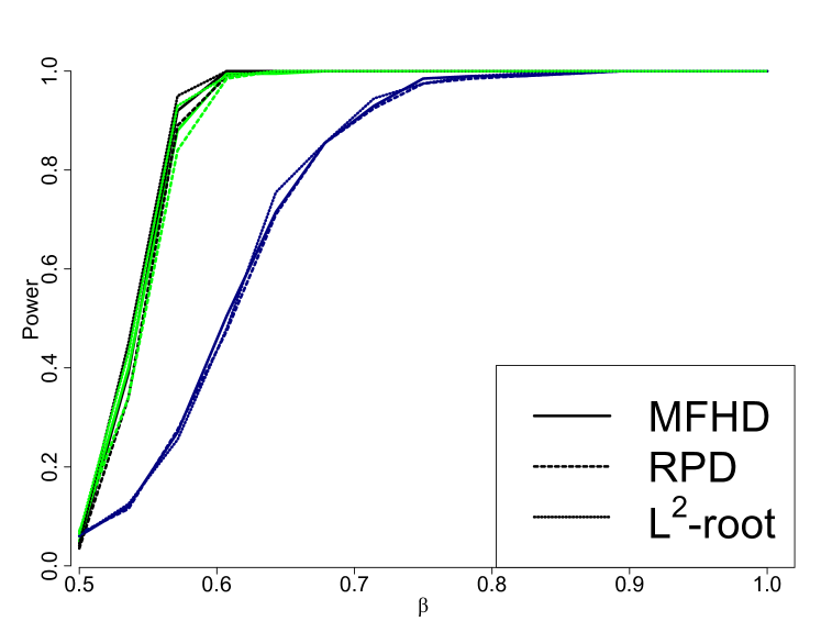
Figure 1: *

(a) magnitude change

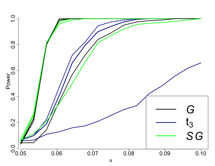
Figure 2: *

(b) shape change

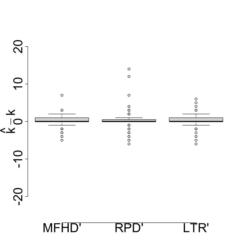
Figure 3: *

(c)

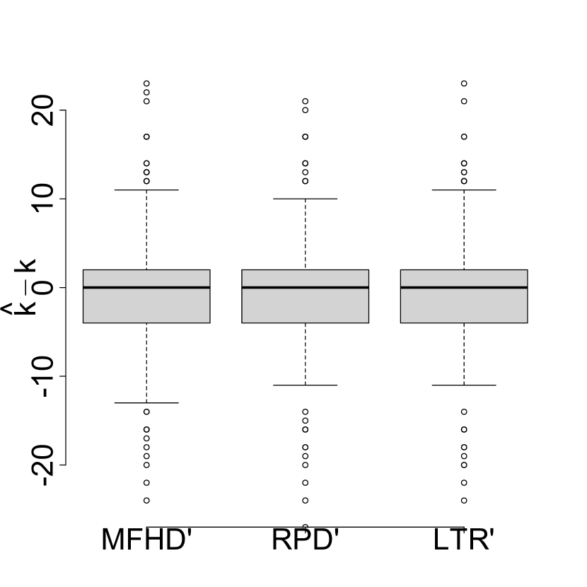
Figure 4: *

(d)

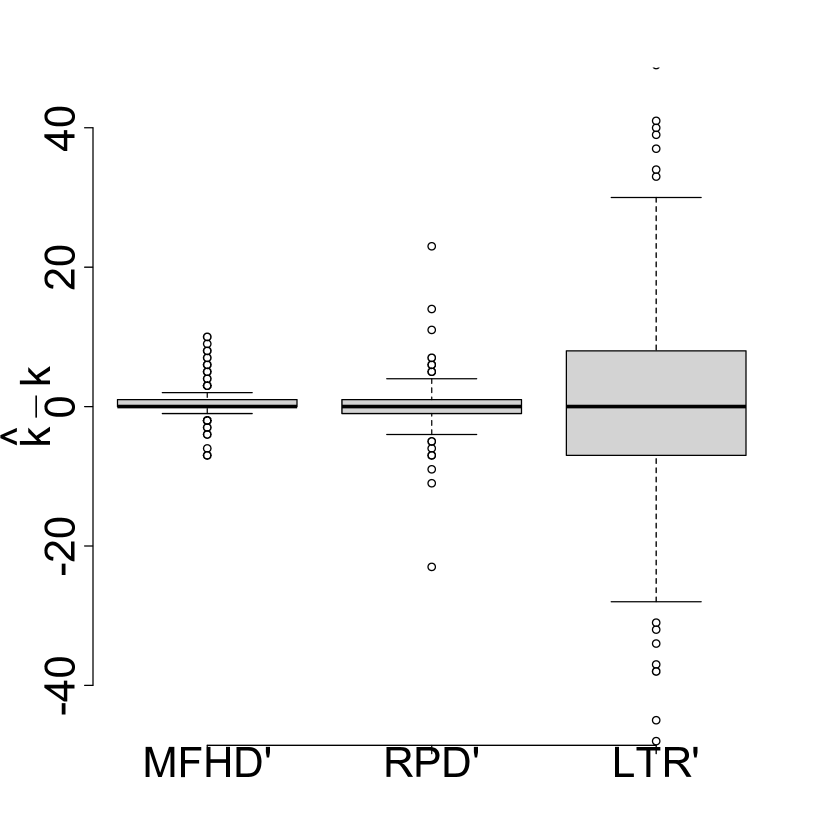
Figure 5: *

(e)

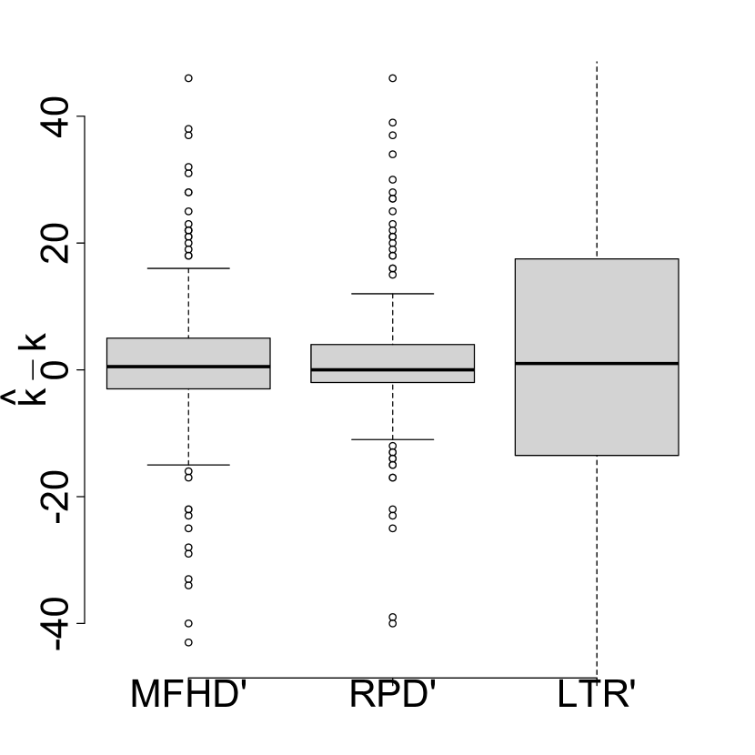
Figure 6: *

(f)

Figure 7: Power curves and accuracy boxplots when there is one change-point in the data and $n=500$. Each curve represents the empirical power of the AMOC FKWC hypothesis test, for a given depth function (line type) when the data had a particular underlying distribution (line color). For example, the solid green line is the power of the procedure paired with the $\operatorname{MFHD}$ depth when the data came from a skewed Gaussian process. The boxplots represent the empirical distribution of $\hat{k}-k$ based on the 200 simulation runs. The data model for each of the boxplots was (c) Gaussian with a magnitude change, (d) student $t$ with a magnitude change, (e) Gaussian with a shape change and (f) student $t$ with a shape change. Note that “$L^{2}$-root” refers to the case where our procedure was paired with the ranks of the sum of the squared norms of the observations and their first derivative.

We discuss the AMOC and epidemic scenarios first, the FKWC methods which include the derivatives performed universally better than those without the derivatives, therefore we only present the results of the FKWC methods which use the derivatives. It should be noted that the $\operatorname{MFHD}$ and squared norm based FKWC procedures cannot detect shape changes without including the derivative information, see Appendix B. We also only present the results from the AMOC runs, since the results from the epidemic scenarios resulted in the same conclusions. The results from the epidemic scenarios can be seen in Appendix B.

Figure 7 shows the power curves for the AMOC FKWC test when the data had magnitude changes (panel (a)) and when the data had shape changes (panel (b)). Here, $n=500$ and the results from other sample sizes were similar. (It was observed that a higher sample size indicates a higher detection power.) Figure 7 shows that the power of the test is lower when the underlying data comes from a heavy tailed distribution, but the method does not break down. We also see that performing the test on skewed Gaussian data performs similarly to when performed on non-skewed Gaussian data. When the change-point altered the shape of the data, using the squared norm-based ranks based did not work as well as the other two depth functions if the data was not Gaussian, even if the derivative information was incorporated. The performance of the test using ranks based on $\operatorname{RPD}^{\prime}$ and $\operatorname{MFHD}^{\prime}$ was similar, with $\operatorname{MFHD}^{\prime}$ being slightly better for magnitude differences and $\operatorname{RPD}^{\prime}$ being slightly better for shape differences. The empirical sizes of the test, were always within $2\%-3\%$ of the nominal size, being within $1\%-2\%$ most of the time. The bottom row of Figure 7 contains boxplots of $\hat{k}_{1}-k_{1}$ when the change-point was detected. We observe again that when the data is heavy tailed, the estimation is less accurate, but still works. For example, the estimated change-point is often within 4 observations instead of 2 when the change-point was a magnitude change. The estimation accuracy results mirror those of the power curves; $\operatorname{RPD}^{\prime}$ and $\operatorname{MFHD}^{\prime}$ perform the best with slight differences depending on whether or not the change type was shape or magnitude.

Figure 10 compares the power of the methods of (Sharipov and Wendler, , 2020; Dette and Kokot, , 2020) to the power of the FKWC methods. We used 200 bootstrap samples with a block length of 1 for both of the competing methods. We only report the results for the integrated test of (Sharipov and Wendler, , 2020), since it had generally higher power than the other test proposed in their paper. For the Dette method, we used 49 b-spline basis functions to smooth the data first and, note that using a Fourier basis resulted in slightly lower power. We did not smooth the data for use with the method of (Sharipov and Wendler, , 2020). It can be seen in Figure 10 that the FKWC test has a higher power than its competitors for the data models in this simulation study. We also notice that the heavy tailed distribution breaks down the competing methods. We remark that though the FKWC methods have higher power than competing methods under these simulation models, the competing methods have some features that the FKWC methods do not. These methods have theoretical results for dependent data and the method by Dette and Kokot, (2020) can test for “relevant” changes in the covariance operator, rather than the standard hypothesis of any change in the covariance operator.

In order to test the performance of the FKWC tests when the data are not independent, we also compared the three tests under a model where the data had some dependency. We simulated functions from the autoregressive model as discussed in the simulation section of (Sharipov and Wendler, , 2020) and ran the FKWC test on those time series. Table 3 in Appendix B shows the results under this model. We see that the FKWC tests (which incorporate the derivatives) have higher power than competing methods, though they tend to have higher type one error. The $\operatorname{RPD}^{\prime}$ test is an exception; it had an empirical size of 0.06, which is very close to the nominal level of 0.05. Overall, the performance of the FKWC test is better than its competitors under these simulation models.

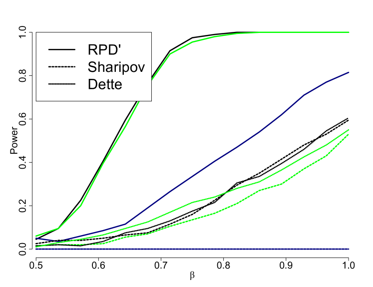
Figure 8: *

(a)

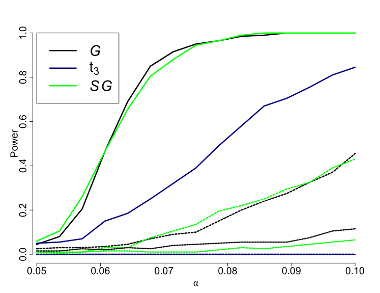
Figure 9: *

(b)

Figure 10: Power curves of the FKWC method compared to the methods of (Sharipov and Wendler, , 2020; Dette and Kokot, , 2020) when there was one change-point in the data and $n=100$. Each curve represents the empirical power of a particular change-point procedure when the data had a particular distribution. For example, a green curve with a dashed line is the empirical power curve of the method of (Sharipov and Wendler, , 2020) when the data was generated from a skewed Gaussian process.

We now discuss the results from the multiple change-point algorithm. When there were five change-points, we ran four different simulation scenarios, two where the change-points were shape-type and two where the changes were magnitude-type. Within these groups, the set of change-points was either “ascending”, i.e., $\alpha$ or $\beta$ was increasing with each change or “alternating”, i.e., $\alpha$ or $\beta$ was oscillating between a high and low value with each change.

We first discuss choosing the value of $\lambda_{n}$. It was observed by Ramsay and Chenouri, (2020) that $\lambda_{n}\in(3.74+0.15\sqrt{n},3.74+0.25\sqrt{n})$ performs well in the multivariate setting. In this study, we tested $\lambda_{n}=3.74+\lambda_{n}^{\prime}\sqrt{n}$ for $\lambda_{n}^{\prime}\in(0.1,0.4)$ to see if the same parameter settings apply to the functional data setting. We ran the PELT algorithm on the simulated data for all of the scenarios, i.e., for data which had 0, 1, 2 and 5 change-points. We observed that the best choice of $\lambda_{n}^{\prime}$ was consistent across the different depth functions, and so we only present the results from $\operatorname{RPD}^{\prime}$ depth. Figure 14 shows the mean absolute error in the estimated amount of change-points, i.e., $|\ell-\hat{\ell}|$, of the simulation scenarios for different values of $\lambda_{n}^{\prime}$ for $n=500$. It is clear that the functional data context requires higher values of $\lambda_{n}^{\prime}$, with the best parameters being in $0.25-0.4$ range. The algorithm is less sensitive to the choice of $\lambda_{n}^{\prime}$ with increased sample sizes. The group of curves presenting large errors at the top of panel (a) of Figure 14 are from the shape difference and/or heavy tailed scenarios with five change-points, where there was not enough samples to detect all of the change-points.

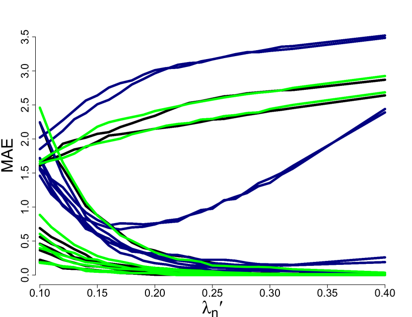
Figure 11: *

(a)

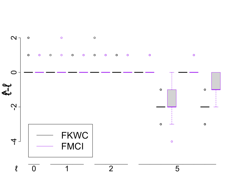
Figure 12: *

(b)

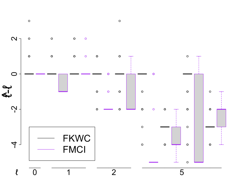
Figure 13: *

(c)

Figure 14: (a) Mean absolute error $|\ell-\hat{\ell}|$ of the simulation scenarios for different values of $\lambda_{n}^{\prime}$ under the $\operatorname{RPD}^{\prime}$ depth for $n=500$. (b) Boxplots of $\hat{\ell}-\ell$ when the data contains different amounts of change-points (as labelled on the horizontal axis) under the Gaussian simulation scenario. (c) Boxplots of $\hat{\ell}-\ell$ when the data contains different amounts of change-points under the $t_{3}$ simulation scenario.

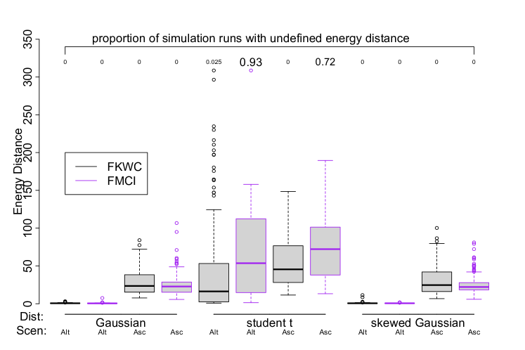
Figure 15: *

Magnitude changes

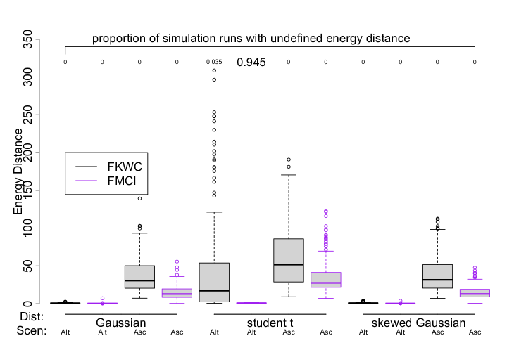
Figure 16: *

Shape changes

Figure 17: Energy distance between the estimated and true change-points when $n=500$ for the FKWC method and the FMCI method. The FKWC method was used with $\operatorname{RPD}^{\prime}$ depth and $\lambda_{n}^{\prime}=0.3$ and the FMCI method was used with the default parameters. Only the runs in which there were five change-points are represented. The numbers at the top of the graph are the proportion of runs in which the algorithm failed to identify any change-points. The labels on the horizontal axis represent the distribution of the underlying data and the change-point scenario; either alternating or ascending.

We now compare the $\operatorname{RPD}^{\prime}$ version of the FKWC multiple change-point method to the FMCI method of Harris et al., (2021). We chose to compare to (Harris et al., , 2021) because of FMCI’s ability to detect multiple change-points, as well as its accessible implementation and computational speed. We use the default parameters provided in the fmci package. We remark that the FMCI method can detect changes in both the mean function and covariance kernel, whereas the FKWC method can only detect changes in the covariance kernel. It should be noted that we used the same simulation to evaluate the best parameter choice for the FKWC method, and so the results could be biased in favor of the FKWC method. We do not feel this plays a major in the conclusions drawn from the comparison.

Figure 14 contains boxplots of $\hat{\ell}-\ell$ for different data models in the simulation. The results of skewed Gaussian and Gaussian were similar so we only present those of Gaussian and student $t$. We see that the results of both methods are similar under the Gaussian setting (while slightly favoring the FMCI method), but favor the FKWC method when the data is heavy tailed. Both methods tend to underestimate the number of change-points in the heavy-tailed case. We observed that both of these methods had more difficulty in the ascending scenarios, i.e., the simulation runs where either the $\alpha$ or $\beta$ parameters were increasing at each change-point.

To evaluate the accuracy of the algorithms, we also look at the energy distance between the estimated change-point set and true change-point set for each method. The energy distance between the estimated and the true change-point set can written as

$$\frac{2}{\hat{\ell}\ell}\sum_{i=1}^{\hat{\ell}}\sum_{j=1}^{\ell}|\hat{k}_{i}-k_{j}|-\frac{1}{\hat{\ell}^{2}}\sum_{i=1}^{\hat{\ell}}\sum_{j=1}^{\hat{\ell}}|\hat{k}_{i}-\hat{k}_{j}|-\frac{1}{\ell^{2}}\sum_{i=1}^{\ell}\sum_{j=1}^{\ell}|k_{i}-k_{j}|.$$

As done by Harris et al., (2021), we use the energy distance to evaluate the multiple change-point methods. We use this distance because, as discussed in Appendix B.3 of (Harris et al., , 2021), the energy distance measures the average error in estimating each change-point, rather than the error of the most poorly estimated change-point in the set. One criticism is that if the algorithm fails to identify any change-points, then the energy distance to a set of true change-points will not be defined.

Figure 17 shows boxplots of the energy distance between the estimated change-point set and true change-point set, for each method. The numbers along the top of the graph indicate the proportion of simulation runs in which the algorithm failed to identify any change-points. Figure 17 shows that the FMCI method performs better in the Gaussian and skewed Gaussian scenarios when the change-points are ‘ascending’. However, the FMCI method can perform poorly in the heavy-tailed scenario. Notice that in the alternating scenario, under the heavy-tailed distribution, the FMCI method fails to identify a change-point over 90% of the time. We conclude that the FMCI method performs better when the data are not heavy tailed, but the FKWC performs better when the data are heavy tailed. In other words, the FKWC method sacrifices some of the accuracy of the FMCI method for robustness to outliers.

5 Data analysis

5.1 Changes in volatility of social media intraday returns

Figure 18: *

(a)

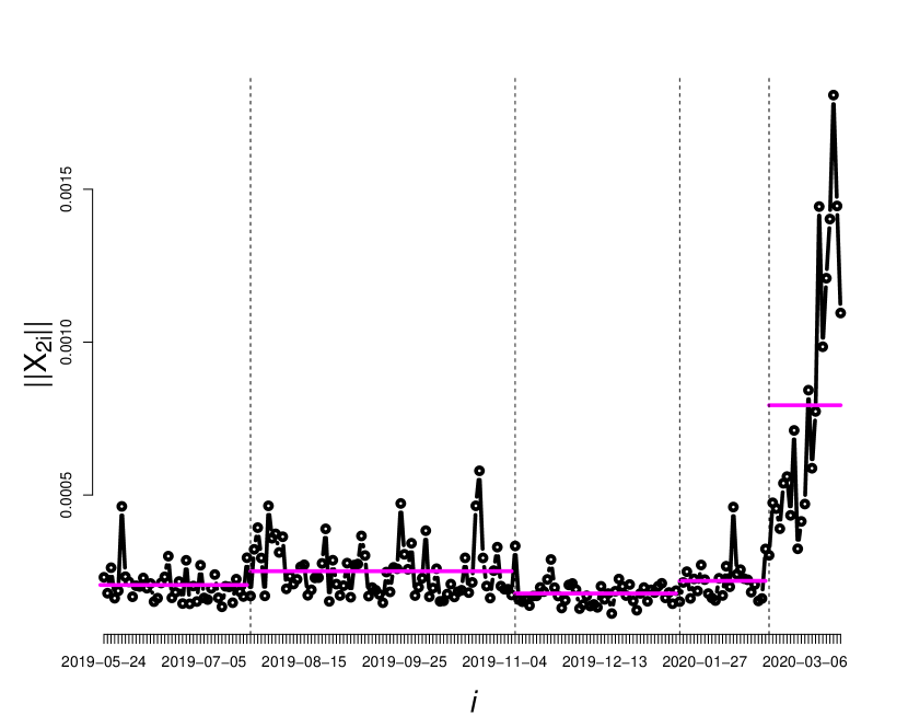
Figure 19: *

(b)

Figure 20: (a) Twitter differenced log returns and (b) norms of the Twitter differenced log returns over time, with the FKWC detected change-points and change-point interval means overlaid.

In this section we present an application of the multiple change-point algorithm to intraday differenced log returns of twtr stock. We analyse 207 daily asset price curves of twtr starting on June 24th 2019 and ending March 20th 2020. The price was measured in one minute intervals, over the course of the trading day, resulting in a total of 390 minutes per day. In order to account for edge effects from smoothing the curves, we trimmed 10% of the minutes from the beginning of the day and 5% of the minutes from the end of the day. This resulted in 332 minutes of stock prices. The differenced log returns are defined as

$$X_{ji}(t)=\ln(Y_{ji\lfloor 331t\rfloor+1})-\ln(Y_{ji\lfloor 331t\rfloor}),$$

for $t\in(0,1]$ and where $Y_{jik}$ is the $j^{th}$ asset price on the $i^{th}$ day at minute $k$. The data was fit to a b-spline basis, using 50 basis functions, see smooth.basis in the fda R package. These data are shown in Figure 20. The assumption of zero mean appears to be satisfied here. Notice the outliers, which indicates that this data may require robust inference. Obviously, these data are not independent, however, we feel that this will not overtly affect our procedure. As long as the intervals between change-points are big enough, we expect the depth values after a change to also change, even if there is say, $m$-dependence in the data. We would expect that $m$-dependence could blur the change for a short period of time and cause the change-point estimate to be biased.

We ran the PELT algorithm with $\lambda_{n}=3.74+0.3\sqrt{n}=8.06$, as per Section 4. We ran the algorithm under all of the depth functions with the derivatives. The FKWC method using the $\operatorname{MFHD}$ depth identified a change-point on Jan 15 ‘20 which the other two depth functions did not. If we include this change-point, the algorithm identified four change-points, as given in Table 1. The algorithm using the ranks of the squared norms without the derivatives identified the same set of change-points. We could then infer that there were change-points in the magnitude of the observations. We remark that other, additional changes in the covariance operator may have also occurred at these times. For example, the magnitude change may also have been accompanied by a change in the shape of the curves.

Figure 20 displays the norms of the curves over time, with the estimated change-points added as vertical lines and the means of the norms in each interval overlaid. We can see clear changes in the mean of the norms during these periods. We may also notice that our procedure was unaffected by the outlier at the beginning of the series and the one just before the last estimated change-point. Table 1 gives the magnitude and sign of the changes as well. We can see that the largest change-point is the last one; clearly attributed to the instability caused by the coronavirus pandemic. It is interesting to see whether or not the other change-points occurred due to market wide behaviour, or events specific to social media or even just Twitter itself. For example, running the same algorithm on snap stock over the same period of time reproduces the change-points on Nov 07 ‘19 and Feb 21 ‘20 but not the other two change-points. One possibility for the estimated change-point on July 2019 could be the Twitter earnings report released just prior, e.g., (Feiner, , 2019).

Aside from determining possible causes for change-points, from a modelling perspective, one may wish to avoid using a functional GARCH model. This could be due to the fact that in order to fit a functional GARCH model at the present time, one must choose to fit the functional data to a relatively small number of basis functions in order to keep to the number of parameters in the GARCH model small. If no clear basis exists, and the principle component analysis does not work well due to outliers, one may wish for an alternate approach. Instead one can remove the heteroskedasticity in the data by re-normalizing the curves in each interval, and then proceed with alternative time series modelling from there. Of course, this would not estimate future change-points; one could model the change-point process and the return curves separately.

Interval	Centered Rank Mean
Jun 24 ‘19 - Jul 24 ‘19	19.73
Jul 24 ‘19- Nov 07 ‘19	-15.64
Nov 11 ‘19- Jan 15 ‘20	46.04
Jan 15 ‘20- Feb 21 ‘20	1.08
Feb 21 ‘20 - Mar 20 ‘20	-90.80

Table 1: Change-points and centered $\operatorname{MFHD}^{\prime}$ rank means. Notice the largest change occurs at the last change-point.

5.2 Resting state f-MRI pre-processing

Functional magnetic resonance imaging, or f-MRI, is a type of imaging for brain activity. f-MRI uses magnetic fields to determine oxygen levels of blood in the brain in order to produce 3-dimensional images of the brain. Many of these images are taken over a period of time, which results in a time series of 3-dimensional images. Note that each MRI in a given subject’s f-MRI can be viewed as a function on $[0,1]^{3}$. Resting state f-MRI is a type of f-MRI data where no intervention is applied to the subject during the scanning process. f-MRI scans go through extensive pre-processing before being analysed.

One assumption commonly made is that, after several pre-processing steps, each subject’s resulting functional time series is stationary. It is therefore important to check the scans at an individual level in order to ensure that each time series is stationary. For subjects whose time series is not stationary, we must make the necessary corrections or exclusions from the ensuing data analysis. The covariance kernel of an f-MRI time series is a 6-dimensional function. Existing methods make a separability assumption on the covariance kernel (Stoehr et al., , 2019), which we do not make here. Additionally, Stoehr et al., (2019) mentions the need for a robust method of detecting non-stationarities in f-MRI data, which leads us to apply our rank based method to this data. We analyse several scans from the Beijing dataset, which were retrieved from www.nitrc.org. These scans were also analysed by Stoehr et al., (2019). Following instruction provided by https://johnmuschelli.com/, we performed the following pre-processing steps to the data. We trimmed the first 10 seconds from the beginning of the scan, in order to have a stable signal. We then performed rigid motion correction using antsMotionCalculation function in the ANTsR R package. A 0.1 Hz high-pass Butterworth filter of order 2 was applied voxel-wise to remove drift and trend from the data. We then removed 15 observations from either end of the time series in order to remove the edge effects of the filter. The gradient of each scan was then estimated using the numDeriv package, which resulted in four time series of functional data, where each function is a three-dimensional image.

We then computed the $\operatorname{RPD}^{\prime}$ sample depth values as follows. First we projected each of the four time series’ onto 50 unit functions. Then, for each of the 50 projected time series, we computed the half-space depth values of each four-dimensional observation. We then averaged these depths over the 50 unit vectors. We use the half-space depth since it is faster to compute than the simplicial depth for four-dimensional data. We then applied the FKWC epidemic test and the FKWC multiple change-point algorithm to the resulting depth values. Code to run the FKWC procedure on three-dimensional functional data can be retrieved from Github (Ramsay, , 2021).

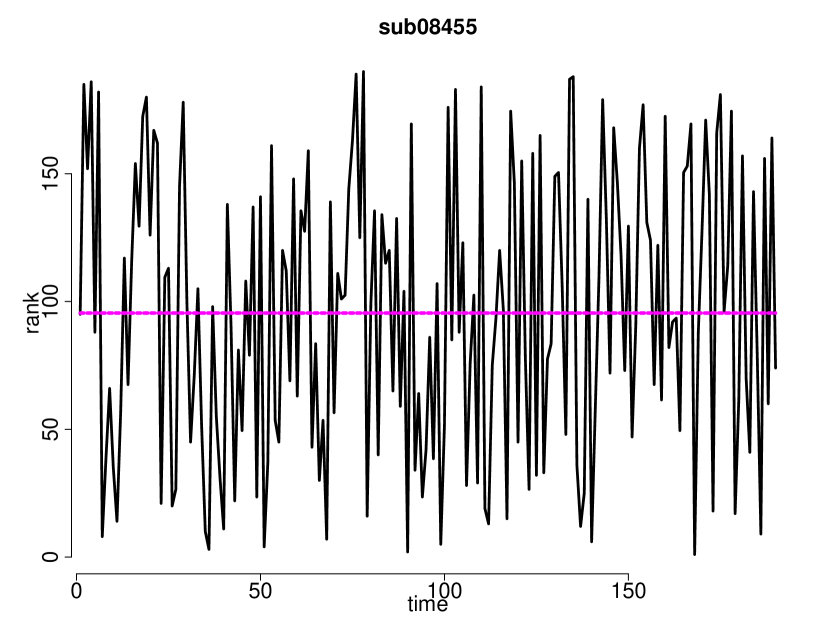
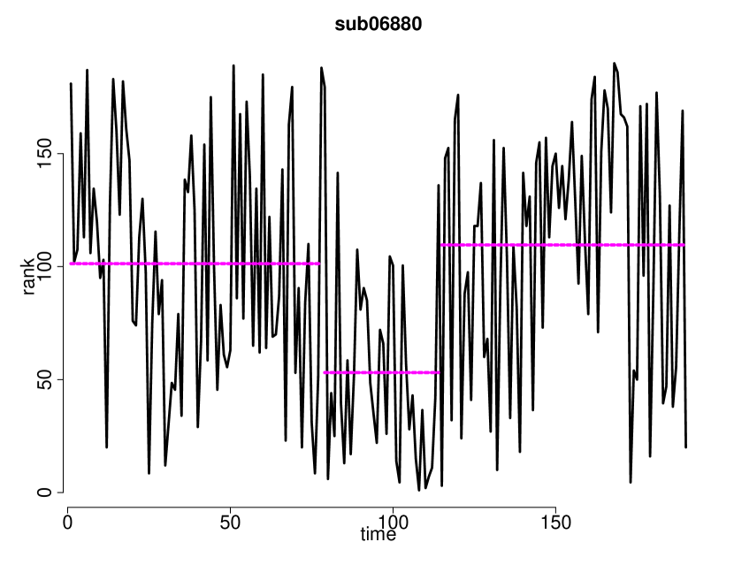
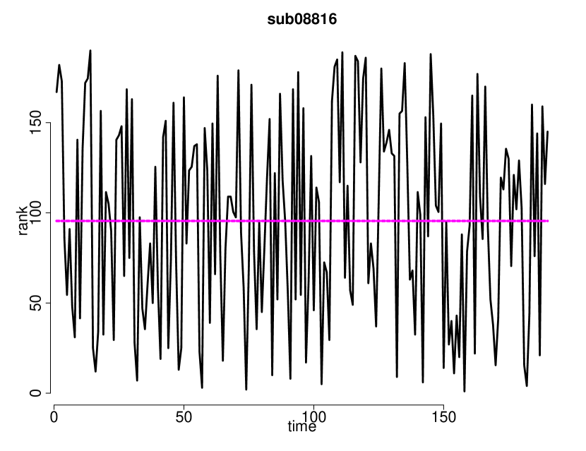
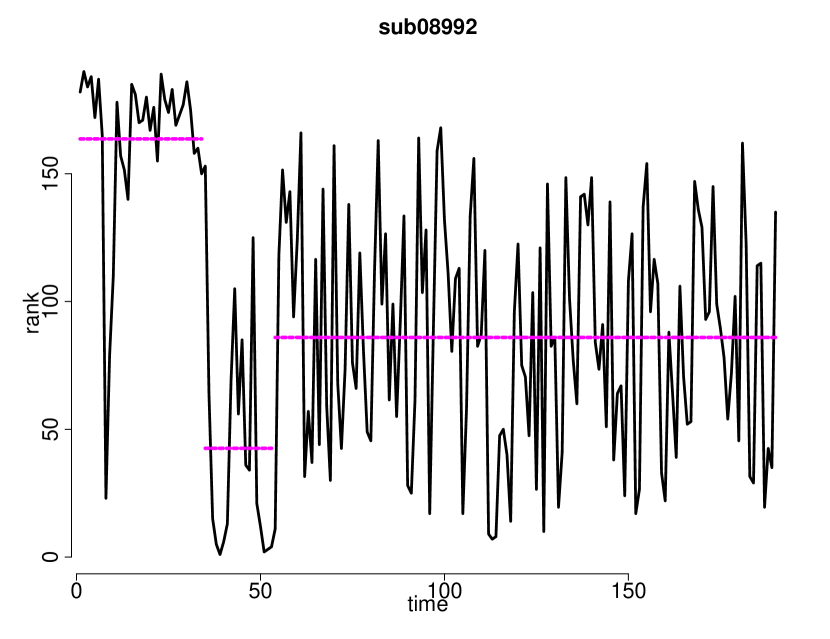
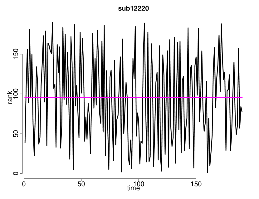
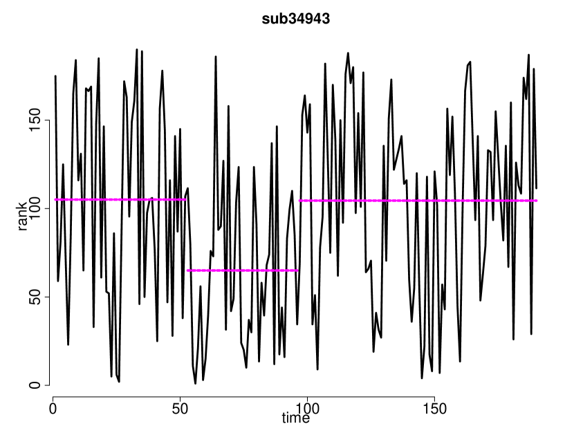
Figure 21: Ranks of the random projection depth values for several f-MRI scans with detected change-point means overlaid.

Figure 21 contains the ranks of the random projection depth values for several f-MRI scans, with the resulting change-point intervals identified by the FKWC multiple change-point algorithm overlaid. We see that changes are detected in three of the six subjects analysed, two of which appear to be an epidemic type change; the ranks return to their previous means after the second interval. This is consistent with the idea that the epidemic model is more suitable for some resting state f-MRI scans (Stoehr et al., , 2019). The rank sequence for subject sub08992 also has two change-points, though the distribution of ranks in the first and third intervals are clearly different. We see that the FKWC procedure ignores the outlier at the beginning of the sequence for subject sub08992, which showcases the robustness of the FKWC method. For subject sub08455, we do not detect any changes in the sequence, even though this subject’s f-MRI has an outlier early in the sequence. This outlier can create a false positive for the AMOC alternative, as discussed by Stoehr et al., (2019). The FKWC method did not detect any change-points for subject sub08816, whereas the methods of (Stoehr et al., , 2019) detected an epidemic period. This could be due to differences in pre-processing, trimming, or the separability assumption. For subject sub12220, the hypothesis test fails to reject the hypothesis of no changes, however the test of (Stoehr et al., , 2019) detects a change. The location of the change detected by Stoehr et al., (2019) occurs early in the sequence, and, as a result of the trimming we applied to the sequence, occurs very early in our time series. This makes it difficult to detect by our procedure. For subject sub34943 we see that a change is detected by the FKWC procedure. We note that no change was detected by the functional procedure in (Stoehr et al., , 2019), but a change was detected in the multivariate procedure.

Appendix A Proofs

Proof of Theorem 1.

The first equation follows from (Chenouri et al., , 2020), and so we only must prove the second equation in the theorem holds. Directly from (Chenouri et al., , 2020), see also (Billingsley, , 1968), we have that

$$\widehat{Z}_{n}(t)=\frac{1}{\sqrt{n}}\sum_{i=1}^{\lfloor tn\rfloor}\frac{\widehat{R}_{i}-(n+1)/2}{\sqrt{\left(n^{2}-1\right)/12}}\stackrel{{\scriptstyle\text{d}}}{{\rightarrow}}B(t),$$

for $t\in[0,1]$. Let $q_{n}=\frac{(n^{2}-1)}{n(n+1)}$, clearly $q_{n}\rightarrow 1$ as $n\rightarrow\infty$. We write $\mathcal{W}$ as a function of the partial sums of similar form of that of $\widehat{Z}_{n}(t)$. Consider the first term in (3). We have that

$$\left(\frac{12}{n(n+1)}\right)^{1/2}\sum_{1\leq j<k_{1}\atop k_{2}\leq j\leq n}^{n}\frac{\widehat{R}_{j}-(n+1)/2}{\sqrt{n-k_{2}+k_{1}}} =\left(\frac{q_{n}}{1-k_{2}/n+k_{1}/n}\right)^{1/2}\frac{1}{\sqrt{n}}\left(\sum_{j=1}^{k_{1}-1}\frac{\widehat{R}_{j}-(n+1)/2}{(n^{2}-1)/12}+\sum_{j=k_{2}}^{n}\frac{\widehat{R}_{j}-(n+1)/2}{(n^{2}-1)/12}\right)$$

$$=\left(\frac{q_{n}}{1-k_{2}/n+k_{1}/n}\right)^{1/2}\frac{1}{\sqrt{n}}\left(\sum_{j=1}^{k_{1}-1}\frac{\widehat{R}_{j}-(n+1)/2}{(n^{2}-1)/12}-\sum_{j=1}^{k_{2}-1}\frac{\widehat{R}_{j}-(n+1)/2}{(n^{2}-1)/12}\right)$$

$$=-\left(\frac{q_{n}}{1-k_{2}/n+k_{1}/n}\right)^{1/2}\frac{1}{\sqrt{n}}\left(\sum_{j=k_{1}}^{k_{2}-1}\frac{\widehat{R}_{j}-(n+1)/2}{(n^{2}-1)/12}\right).$$

For the second term in (3), we have that

$$\left(\frac{12}{n(n+1)}\right)^{1/2}\sum_{j=k_{1}}^{k_{2}-1}\frac{\widehat{R}_{j}-(n+1)/2}{\sqrt{k_{2}-k_{1}}} =\left(\frac{q_{n}}{k_{2}/n-k_{1}/n}\right)^{1/2}\frac{1}{\sqrt{n}}\left(\sum_{j=k_{1}}^{k_{2}-1}\frac{\widehat{R}_{j}-(n+1)/2}{(n^{2}-1)/12}\right).$$

So, it follows that

$$\mathcal{W}(k_{1},k_{2})=\frac{q_{n}}{(k_{2}/n-k_{1}/n)(1-k_{2}/n+k_{1}/n)}\left(\frac{1}{\sqrt{n}}\sum_{j=k_{1}}^{k_{2}-1}\frac{\widehat{R}_{j}-(n+1)/2}{(n^{2}-1)/12}\right)^{2}.$$

We can write $\mathcal{W}$ as a function of $0\leq t_{1}\leq t_{2}\leq 1$ as $\mathcal{W}_{n}(t_{1},t_{2})$, where $k_{1},k_{2}$ are replaced with $\lfloor t_{1}n\rfloor,\ \lfloor t_{2}n\rfloor$ respectively. We can then write

$$\mathcal{W}_{n}(t_{1},t_{2})\coloneqq g_{n}(t_{1},t_{2})\mathcal{W}_{n}^{\prime}(t_{1},t_{2}),$$

where

$$g_{n}(t_{1},t_{2})=\frac{1}{(t_{2}-t_{1})(1-t_{2}+t_{1})}+o(1)\qquad\text{ and }\qquad\mathcal{W}_{n}^{\prime}(t_{1},t_{2})=\left(\frac{1}{\sqrt{n}}\left(\sum_{j=\lfloor nt_{1}\rfloor}^{\lfloor nt_{2}\rfloor-1}\frac{\widehat{R}_{j}-(n+1)/2}{(n^{2}-1)/12}\right)\right)^{2}.$$

Recall that $\widehat{Z}_{n}(t)\stackrel{{\scriptstyle\text{d}}}{{\rightarrow}}B(t)$, and it is also clear that $\mathcal{W}_{n}^{\prime}(t_{1},t_{2})=(\widehat{Z}_{n}(t_{1})-\widehat{Z}_{n}(t_{2}))^{2}$. $\mathcal{W}_{n}^{\prime}(t_{1},t_{2})$ is a continuous functional of $\widehat{Z}_{n}(t)$, and so continuous mapping theorem gives that

$$\mathcal{W}_{n}^{\prime}(t_{1},t_{2})=\left(\frac{1}{\sqrt{n}}\left(\sum_{j=\lfloor nt_{1}\rfloor}^{\lfloor nt_{2}\rfloor-1}\frac{\widehat{R}_{j}-(n+1)/2}{(n^{2}-1)/12}\right)\right)^{2}\stackrel{{\scriptstyle\text{d}}}{{\rightarrow}}(B(t_{2})-B(t_{1}))^{2}.$$

and

$$\sup_{t_{1}<t_{2}}\mathcal{W}((\lfloor nt_{1}\rfloor,\lfloor nt_{2}\rfloor))\stackrel{{\scriptstyle\text{d}}}{{\rightarrow}}\sup_{t_{1}<t_{2}}\left(\frac{1}{(t_{2}-t_{1})(1-t_{2}+t_{1})}\right)(B(t_{2})-B(t_{1}))^{2}.$$

∎

Lemma 1.

Suppose that there are $n$, independent univariate data points, with a change-point at observation $k_{1}$. Let $R_{1},\ldots,R_{k_{1}}$ denote the first $k_{1}$ combined sample ranks. For $1\leq m<k_{1}$ and $\delta>0$, consider $S_{m}=\sum_{i=1}^{m}R_{i}$. Then,

$$\Pr(|S_{m}-{\rm{E}}\left[S_{m}\right]|>\delta)\leq 2e^{-2\min(m,k_{1}-m,n-k_{1})\left(\frac{\delta}{2\max(k_{1}-m,n-k_{1})m}\right)^{2}}.$$

Proof.

Let $P(X_{1}>X_{n})=p$. It holds that

$$S_{m} =\sum_{j=1}^{m}R_{j}$$

$$=\frac{m(m+1)}{2}+\sum_{j=1}^{m}\sum_{i=m+1}^{k_{1}}\mathbbm{1}(X_{j}\leq X_{i})+\sum_{j=1}^{m}\sum_{i=k_{1}+1}^{n}\mathbbm{1}(X_{j}\leq X_{i})$$

$$\coloneqq\frac{m(m+1)}{2}+(k_{1}-m)mU^{1}_{n}+m(n-k_{1})U^{2}_{n},$$

where $U^{1}_{2},\ U^{2}_{n}$ are two sample U-statistics. Note that ${\rm{E}}\left[U^{1}_{2}\right]=1/2$ and ${\rm{E}}\left[U^{1}_{2}\right]=p$. We make use of (Hoeffding, , 1963) which gives, for a two sample U-statistic $U$ related to the sample sizes $n_{1}$ and $n_{2}$,

$$\Pr(|U-{\rm{E}}\left[U\right]|>\delta)\leq 2e^{-2\min(n_{1},n_{2})t^{2}}.$$ (9)

Continuing,

$$\Pr(S_{m}-{\rm{E}}\left[S_{m}\right]>\delta) =\Pr\left(({k_{1}}-m)m(U^{1}_{n}-1/2)+m(n-{k_{1}})(U^{2}_{n}-p)>\delta\right)$$

$$\leq\Pr\left(U^{1}_{n}-1/2>\frac{\delta}{2({k_{1}}-m)m}\right)+\Pr\left(U^{2}_{n}-p>\frac{\delta}{2m(n-{k_{1}})}\right)$$

$$\leq e^{-2\min(m,{k_{1}}-m)\left(\frac{\delta}{2({k_{1}}-m)m}\right)^{2}}+e^{-2\min(m,n-{k_{1}})\left(\frac{\delta}{2m(n-{k_{1}})}\right)^{2}}$$

$$\leq e^{-2\min(m,{k_{1}}-m,n-{k_{1}})\left(\frac{\delta}{2\max({k_{1}}-m,n-{k_{1}})m}\right)^{2}}.$$

Note that taking

$$\Pr(|S_{m}-{\rm{E}}\left[S_{m}\right]|>\delta)\leq\Pr(S_{m}-{\rm{E}}\left[S_{m}\right]>\delta)+\Pr(-S_{m}+{\rm{E}}\left[S_{m}\right]>\delta),$$

and $-S_{m}+{\rm{E}}\left[S_{m}\right]$ has the same U-statistic format as $S_{m}-{\rm{E}}\left[S_{m}\right]$. Thus, the previous analysis applies and we get

$$\Pr(|S_{m}-{\rm{E}}\left[S_{m}\right]|>\delta)\leq 2e^{-2\min(m,{k_{1}}-m,n-{k_{1}})\left(\frac{\delta}{2\max({k_{1}}-m,n-{k_{1}})m}\right)^{2}}.$$

∎

Lemma 2.

Suppose that there are $n$ univariate data points, with a change-point at observation $k_{1}$. Let $R_{1},\ldots,R_{k_{1}}$ denote the first $k_{1}$ combined sample ranks, let $\sigma_{n}=\sqrt{(n^{2}-1)/12}$, let $\mu_{n}=(n+1)/2$ and let

$$Z_{n}(t)=\frac{1}{\sqrt{n}}\sum_{i=1}^{\lfloor tn\rfloor}\frac{R_{i}-\mu_{n}}{\sigma_{n}}.$$

It holds that

$$\Pr(Z_{n}(k_{1}/n)<a_{n})\leq e^{-2n\min(\theta_{1},1-\theta_{1})\left(p-1/2-\frac{a_{n}\sigma_{n}}{n^{2}\theta_{1}(1-\theta_{1})}\right)^{2}},$$

for $a_{n}<\frac{k_{1}(n-k_{1})(p-1/2)}{\sigma_{n}}$ and $k_{1}=\lfloor n\theta_{1}\rfloor$.

Proof.

Note that

$${\rm{E}}\left[Z_{n}({k_{1}}/n)\right] =\frac{{k_{1}}({k_{1}}+1)}{2\sigma_{n}}+\frac{{k_{1}}(n-{k_{1}})p}{\sigma_{n}}-\frac{{k_{1}}(n+1)}{2\sigma_{n}}={k_{1}}(n-{k_{1}})\frac{p-1/2}{\sigma_{n}}.$$

We then have that

$$Z_{n}({k_{1}}/n)=\frac{{k_{1}}({k_{1}}+1)}{2\sigma_{n}}+\frac{{k_{1}}(n-{k_{1}})}{\sigma_{n}}U^{\prime}-\frac{{k_{1}}(n+1)}{2\sigma_{n}},$$

where $U^{\prime}$ is a two sample U-statistic. We then have that

$$\Pr(-Z_{n}({k_{1}}/n)+{\rm{E}}\left[Z_{n}({k_{1}}/n)\right]>t)\leq e^{-2n\min(\theta,1-\theta)\left(\frac{t\sigma_{n}}{{k_{1}}(n-{k_{1}})}\right)^{2}},$$

for $t>0$ (Hoeffding, , 1963; Pitcan, , 2017). Using this fact,

$$\Pr(Z_{n}({k_{1}}/n)<a_{n}) =\Pr\left(Z_{n}({k_{1}}/n)-{\rm{E}}\left[Z_{n}({k_{1}}/n)\right]<a_{n}-{k_{1}}(n-{k_{1}})\frac{p-1/2}{\sigma_{n}}\right)$$

$$=\Pr\left({\rm{E}}\left[Z_{n}({k_{1}}/n)\right]-Z_{n}({k_{1}}/n)>{k_{1}}(n-{k_{1}})\frac{p-1/2}{\sigma_{n}}-a_{n}\right)$$

$$\leq e^{-2n\min(\theta,1-\theta)\left(p-1/2-\frac{a_{n}\sigma_{n}}{n^{2}\theta(1-\theta)}\right)^{2}}$$

where the second line uses the fact that

$$a_{n}-{k_{1}}(n-{k_{1}})\frac{p-1/2}{\sigma_{n}}<0.$$

∎

Theorem 3.

The outline of our proof follows that of the proofs in (Yu and Chen, , 2017), but the details differ since we are using ranks. To keep the notation simple, we let $k_{1}=k$ and $\hat{k}_{1}=\hat{k}$ for the remainder of the proof. Let $\sigma_{n}=\sqrt{(n^{2}-1)/12}$ and $\mu_{n}=(n+1)/2$. The aim is to show that $\Pr(|\hat{k}-k|>tn)<C_{1}\exp(-nt^{2}C_{2})$. To start, note that

$$\Pr(|\hat{k}-k|>tn)=\Pr(\hat{k}-k>tn)+\Pr(k-\hat{k}>tn).$$ (10)

We start with showing a bound on $\Pr(k-\hat{k}>tn)$. Note that

$$\Pr(k-\hat{k}>tn) \leq\Pr\left(\max_{c_{0}n\leq i<k-tn}|Z_{n}(i/n)|>|Z_{n}(k/n)|\right)$$

$$\leq\Pr\left(\max_{c_{0}n\leq i<k-tn}|Z_{n}(i/n)|>Z_{n}(k/n)\right)$$

$$\leq\Pr\left(\max_{c_{0}n\leq i<k-tn}|Z_{n}(i/n)|-Z_{n}(k/n)>0\right)$$

$$\leq\Pr\left(\max_{c_{0}n\leq i<k-tn}Z_{n}(i/n)-Z_{n}(k/n)>0\right)+\Pr\left(\min_{c_{0}n\leq i<k-tn}Z_{n}(i/n)+Z_{n}(k/n)<0\right)$$ (11)

$$\coloneqq\Pr(A_{1})+\Pr(A_{2}).$$ (12)

First consider event $A_{1}$:

$$\Pr(A_{1}) =\Pr\left(\max_{c_{0}n\leq i<k-tn}Z_{n}(i/n)-Z_{n}(k/n)>0\right)$$

$$=\Pr\left(\max_{c_{0}n\leq i<k-tn}-\sum_{j=i+1}^{k}\frac{R_{j}-\mu_{n}}{\sigma_{n}}>0\right)$$

$$=\Pr\left(\max_{tn\leq i<k-c_{0}n}-Z_{n}(i/n)>0\right),$$

where the last line follows from exchangeability of $R_{1},\ldots,R_{k}$. WLOG we can assume that

$$\max_{tn\leq i<k-c_{0}n}-Z_{n}(i/n)=-Z_{n}(i^{*}/n),$$

occurs for some $i^{*}$. Then, in order for $\{\max_{tn\leq i<k-c_{0}n}-Z_{n}(i/n)>0\}$ to also occur, we must have

$$-Z_{n}(i^{*}/n)+{\rm{E}}\left[Z_{n}(i^{*}/n)\right]>{\rm{E}}\left[Z_{n}(i^{*}/n)\right].$$

We will make use of this fact shortly, but first it helps compute ${\rm{E}}\left[Z_{n}(i/n)\right]$. At this point, it is helpful to recall from the proof of Lemma 1 that $Z_{n}(i/n)$ can be written in terms of a generalised, two sample U-statistic. It follows that

$${\rm{E}}\left[Z_{n}(i/n)\right] =\frac{i(i+1)}{2\sigma_{n}}+\frac{i(k-i)}{2\sigma_{n}}+pi(n-k)-i\frac{n+1}{2\sigma_{n}}$$

$$=\frac{i}{\sigma_{n}}(n-k)\left(p-\frac{1}{2}\right)$$

$$\geq\frac{tn}{\sigma_{n}}(n-k)\left(p-\frac{1}{2}\right),$$

for $tn\leq i<k-c_{0}n$. Pruss, (1998) provides a maximal inequality for sums of exchangeable random variables. Note that we can extend the sequence $R_{1},\ldots,R_{k-c_{0}n}$ to one of length $k$. Which, in the notation of Pruss, (1998), means that $\gamma=k/(k-c_{0}n)=\theta/(\theta-c_{0})$ and we have that

$$c(\gamma)=C_{3}\frac{\gamma^{2}}{(\gamma-1)^{2}}=C_{3}\frac{\theta^{2}}{c_{0}^{2}},$$

where $C_{3}$ is an absolute constant. We can now apply Theorem 1 of (Pruss, , 1998) and Lemma 1, which gives that

$$\Pr\left(\max_{tn\leq i<k-c_{0}n}-Z_{n}(i/n)>0\right) \leq\Pr\left(\max_{tn\leq i<k-c_{0}n}-Z_{n}(i/n)+{\rm{E}}\left[Z_{n}(i/n)\right]>\frac{(n-k)tn}{\sigma_{n}}\left(p-\frac{1}{2}\right)\right)$$

$$\leq C_{3}\frac{\theta^{2}}{c_{0}^{2}}\Pr\left(|Z_{n}(\theta-c_{0})-{\rm{E}}\left[Z_{n}(\theta-c_{0})\right]|>\frac{(n-k)tnc_{0}^{2}}{C_{3}\theta^{2}\sigma_{n}}\left(p-\frac{1}{2}\right)\right)$$

$$\leq 2C_{1}\frac{\theta^{2}}{c_{0}^{2}}e^{-2\min(n(\theta-c_{0}),n-k)\left(\frac{\frac{(n-k)tnc_{0}^{2}}{C_{3}\theta^{2}}\left(p-\frac{1}{2}\right)}{2(n-k)n(\theta-c_{0})}\right)^{2}}$$

$$=2C_{3}\frac{\theta^{2}}{c_{0}^{2}}e^{-2\min(n(\theta-c_{0}),n-k)\left(\frac{tc_{0}^{2}\left(p-\frac{1}{2}\right)}{2C_{1}\theta^{2}(\theta-c_{0})}\right)^{2}}$$

$$=2C_{3}\frac{\theta^{2}}{c_{0}^{2}}e^{-2n\min(\theta-c_{0},1-\theta)\left(\frac{tc_{0}^{2}\left(p-\frac{1}{2}\right)}{2C_{1}\theta^{2}(\theta-c_{0})}\right)^{2}}.$$

We can now show a similar bound for $\Pr(A_{2}).$ To this end, we have that

$$\Pr(A_{2}) =\Pr\left(\max_{c_{0}n\leq i<k-tn}-Z_{n}(i/n)-Z_{n}(k/n)>0\right)$$

$$\leq\Pr\left(\max_{c_{0}n\leq i<k-tn}-Z_{n}(i/n)>0\right)+\Pr\left(Z_{n}(k/n)<0\right).$$

Now, it is easy to see that $\Pr\left(Z_{n}(k/n)<0\right)$ is quite small, viz.

$$\Pr\left(Z_{n}(k/n)<0\right) \leq e^{-2n\min(\theta,1-\theta)\left(p-1/2\right)^{2}},$$

from Lemma 2. Concerning $\Pr\left(\max_{c_{0}n\leq i<k-tn}-Z_{n}(i/n)>0\right)$, we use Corollary 2 of (Pruss, , 1998). Again, in the notation of Pruss, (1998), we take $\rho=c_{0}$ and

$$c(\rho)=c(c_{0})=C_{4}\frac{1}{c_{0}(1-c_{0})^{2}},$$

for some absolute constant $C_{4}$. It follows that

$$\Pr\left(\max_{c_{0}n\leq i<k-tn}-Z_{n}(i/n)>0\right) \leq\Pr\left(\max_{c_{0}n\leq i<k-tn}-Z_{n}(i/n)+{\rm{E}}\left[Z_{n}(i/n)\right]>\frac{c_{0}n(n-k)}{\sigma_{n}}(p-1/2)\right)$$

$$\leq c(c_{0})\Pr\left(|Z_{n}(\theta)-{\rm{E}}\left[Z_{n}(\theta)\right]|>\frac{tc_{0}n(n-k)}{\sigma_{n}c(c_{0})}(p-1/2)\right)$$

$$\leq 2c(c_{0})e^{-2n\min(\theta,1-\theta)\left(\frac{tc_{0}}{\theta c(c_{0})}\right)^{2}(p-1/2)^{2}}.$$

To conclude this part of the proof, we have that

$$\Pr(k-\hat{k}>tn) \leq 2C_{1}\frac{\theta^{2}}{c_{0}^{2}}e^{-2n\min(\theta-c_{0},1-\theta)\left(\frac{tc_{0}^{2}\left(p-\frac{1}{2}\right)}{2C_{3}\theta^{2}(\theta-c_{0})}\right)^{2}}$$

$$\qquad\qquad+e^{-2n\min(\theta,1-\theta)\left(p-1/2\right)^{2}}+2c(c_{0})e^{-2n\min(\theta,1-\theta)\left(\frac{tc_{0}}{\theta c(c_{0})}\right)^{2}(p-1/2)^{2}}$$

$$\leq C_{5}(\theta,c_{0})e^{-2nt^{2}(p-1/2)^{2}C_{6}(\theta,c_{0})}$$ (13)

where $C_{5}(\theta,c_{0})=\max\left(2C_{3}\frac{\theta^{2}}{c_{0}^{2}},2c(c_{0}),1\right)$ and

$$C_{6}(\theta,c_{0})=\min(\theta-c_{0},1-\theta)\min\left[\left(\frac{c_{0}^{2}}{2C_{3}\theta^{2}(\theta-c_{0})}\right)^{2},\left(\frac{c_{0}}{\theta c(c_{0})}\right)^{2},1\right].$$

It now remains to consider $\Pr(\hat{k}-k>tn)$. We have that

$$\Pr(\hat{k}-k>tn) \leq\Pr\left(\max_{k+tn\leq i<n}|Z_{n}(i/n)|>|Z_{n}(k/n)|\right)$$

$$\leq\Pr\left(\max_{k+tn\leq i<n}|Z_{n}(i/n)|>Z_{n}(k/n)\right)$$

$$\leq\Pr\left(\max_{k+tn\leq i<n}|Z_{n}(i/n)|-Z_{n}(k/n)>0\right)$$

$$\leq\Pr\left(\max_{k+tn\leq i<n}Z_{n}(i/n)-Z_{n}(k/n)>0\right)+\Pr\left(\min_{k+tn\leq i<n}Z_{n}(i/n)+Z_{n}(k/n)<0\right)$$

$$\coloneqq\Pr(A_{3})+\Pr(A_{4}).$$

Once again, we start with $\Pr(A_{3})$. Observe

$$\Pr(A_{3}) =\Pr\left(\max_{k+tn\leq i<n}Z_{n}(i/n)-Z_{n}(k/n)>0\right)$$

$$=\Pr\left(\max_{k+tn\leq i<n}\sum_{j=k+1}^{i}\frac{R_{j}-\mu_{n}}{\sigma_{n}}>0\right).$$

Now, note that

$${\rm{E}}\left[-\sum_{j=k+1}^{i}\frac{R_{j}-\mu_{n}}{\sigma_{n}}\right] =(i-k)k\frac{(p-1/2)}{\sigma_{n}}>tnk\frac{(p-1/2)}{\sigma_{n}}.$$

So, it follows that

$$\Pr\left(\max_{k+tn\leq i<n}\sum_{j=k+1}^{i}\frac{R_{j}-\mu_{n}}{\sigma_{n}}>0\right) \leq\Pr\left(\max_{k+tn\leq i<n}\sum_{j=k+1}^{i}\frac{R_{j}-\mu_{n}}{\sigma_{n}}-{\rm{E}}\left[\sum_{j=k+1}^{i}\frac{R_{j}-\mu_{n}}{\sigma_{n}}\right]>tnk\frac{(p-1/2)}{\sigma_{n}}\right)$$

$$\leq c(c_{0})\Pr\left(\left|\sum_{j=k+1}^{k+c_{0}n}\frac{R_{j}-\mu_{n}}{\sigma_{n}}-{\rm{E}}\left[\sum_{j=k+1}^{i}\frac{R_{j}-\mu_{n}}{\sigma_{n}}\right]\right|>\frac{tnk(p-1/2)}{\sigma_{n}c(c_{0})}\right).$$

It is then useful to show that

$$\sum_{j=k+1}^{k+c_{0}n}R_{j}=\frac{c_{0}n(c_{0}n+1)}{2}+c_{0}n(n-c_{0}n-k)V_{1}+c_{0}nkV_{2},$$

where $V_{1},V_{2}$ are two sample U-statistics. As above, we have that

$$\Pr\left(\left|\sum_{j=k+1}^{k+c_{0}n}\frac{R_{j}-\mu_{n}}{\sigma_{n}}-{\rm{E}}\left[\sum_{j=k+1}^{i}\frac{R_{j}-\mu_{n}}{\sigma_{n}}\right]\right|>\delta\right) \leq 2e^{-2n\min(1-c_{0}-\theta,c_{0})\left(\frac{\delta\sigma_{n}}{2c_{0}n(n-c_{0}n-k)}\right)^{2}}+2e^{-2nc_{0}\left(\frac{\delta\sigma_{n}}{2c_{0}n(k)}\right)^{2}}$$

$$\leq 2e^{-2nc_{0}\left(\frac{\delta\sigma_{n}}{2c_{0}n\max(n-k-c_{0}n,k)}\right)^{2}}.$$

It then follows from the proof of Lemma 1 that

$$c(c_{0})\Pr\left(\left|\sum_{j=k+1}^{k+c_{0}n}\frac{R_{j}-\mu_{n}}{\sigma_{n}}-{\rm{E}}\left[\sum_{j=k+1}^{i}\frac{R_{j}-\mu_{n}}{\sigma_{n}}\right]\right|>\frac{tnk(p-1/2)}{c(c_{0})\sigma_{n}}\right)\leq 2c(c_{0})e^{-2nc_{0}\left(\frac{tnk(p-1/2)}{2c_{0}c(c_{0})n\max(n-k-c_{0}n,k)}\right)^{2}}.$$

Consider now,

$$\Pr(A_{4}) =\Pr\left(\max_{k+tn\leq i<n}-Z_{n}(i/n)-Z_{n}(k/n)>0\right)$$

$$=\Pr\left(\max_{k+tn\leq i<n}-\sum_{j=k+1}^{k+i}\frac{R_{j}-\mu_{n}}{\sigma_{n}}>2Z_{n}(k/n)\right)$$

$$\leq\Pr\left(\max_{k+tn\leq i<n}-\sum_{j=k+1}^{k+i}\frac{R_{j}-\mu_{n}}{\sigma_{n}}>2a_{n}\right)+\Pr\left(Z_{n}(k/n)<a_{n}\right)$$

$$\leq\Pr\left(\max_{k+tn\leq i<n}-\sum_{j=k+1}^{k+i}\frac{R_{j}-\mu_{n}}{\sigma_{n}}>2a_{n}\right)+e^{-2n\min(\theta,1-\theta)\left(p-1/2-\frac{a_{n}\sigma_{n}}{n^{2}\theta(1-\theta)}\right)^{2}}.$$

The last line is an application of Lemma 2 if $c_{3}n=2a_{n}<2\frac{k(n-k)(p-1/2)}{\sigma_{n}}$.

$$\Pr\left(\max_{k+tn\leq i<n}-\sum_{j=k+1}^{k+i}\frac{R_{j}-\mu_{n}}{\sigma_{n}}>c_{3}n\right) \leq\Pr\left(\max_{k+tn\leq i<n}-\sum_{j=k+1}^{k+i}\frac{R_{j}-\mu_{n}}{\sigma_{n}}+{\rm{E}}\left[\sum_{j=k+1}^{i}\frac{R_{j}-\mu_{n}}{\sigma_{n}}\right]>c_{3}n-(n-k)k\frac{(p-1/2)}{\sigma_{n}}\right),$$

$$\leq\Pr\left(\max_{k+tn\leq i<n}-\sum_{j=k+1}^{k+i}\frac{R_{j}-\mu_{n}}{\sigma_{n}}+{\rm{E}}\left[\sum_{j=k+1}^{i}\frac{R_{j}-\mu_{n}}{\sigma_{n}}\right]>(n-k)k\frac{(p-1/2)}{2\sigma_{n}}\right),$$

$$\leq 2c(c_{0})e^{-2nc_{0}\left(\frac{(n-k)k(p-1/2)}{4c_{0}c(c_{0})n\max(n-k-c_{0}n,k)}\right)^{2}},$$

which follows from choosing $a_{n}=3\frac{k(n-k)(p-1/2)}{4\sigma_{n}}$. We then have that

$$\Pr(\hat{k}-k>tn) \leq 2c(c_{0})e^{-2nc_{0}\left(\frac{(n-k)k(p-1/2)}{4c_{0}c(c_{0})n\max(n-k-c_{0}n,k)}\right)^{2}}+e^{-9n\min(\theta,1-\theta)\left(p-1/2\right)^{2}/8}$$

$$\qquad\qquad 2c(c_{0})e^{-2nc_{0}\left(\frac{tnk(p-1/2)}{2c_{0}c(c_{0})n\max(n-k-c_{0}n,k)}\right)^{2}}$$

$$\leq\max(2c(c_{0}),1)e^{-nt^{2}(p-1/2)^{2}C_{7}(\theta,c_{0})},$$ (14)

where $C_{7}(\theta,c_{0})=\min\left(2c_{0}\left[\frac{\theta}{4c_{0}c(c_{0})\max(1-\theta-c_{0},\theta)}\right]^{2},\min(\theta,1-\theta)9/8\right)$. Therefore, combining (14) and (13) we have that

$$\Pr(|\hat{k}-k|>tn)\leq C_{5}(\theta,c_{0})e^{-nt^{2}(p-1/2)^{2}C_{8}(\theta,c_{0})},$$

where,

$$C_{8}(\theta,c_{0}) =\min\Bigg{[}\min(\theta-c_{0},1-\theta)\left(\frac{c_{0}^{2}}{2C_{1}\theta^{2}(\theta-c_{0})}\right)^{2},\min(\theta-c_{0},1-\theta)\left(\frac{c_{0}}{\theta c(c_{0})}\right)^{2},$$

$$\qquad\min(\theta-c_{0},1-\theta),2c_{0}\left[\frac{\theta}{4c_{0}c(c_{0})\max(1-\theta-c_{0},\theta)}\right]^{2},\min(\theta,1-\theta)9/8\Bigg{]}.$$

∎

Lemma 3.

Suppose that $\hat{S}_{m}=\sum_{j=1}^{m}\widehat{R}_{j}$; the sum of the ranks based on the sample depth functions for some $m\leq k_{1}$. Assume the conditions of Theorem 4. We have that

$$\Pr\left(\frac{1}{m}\hat{S}_{m}-\frac{1}{m}S_{m}>t\right)\leq K_{1}e^{-K_{2}\min(m,n-k_{1},k_{1}-m)t^{2}},$$

for some constants $K_{1},K_{2}$ that depend on $b,\ K^{\prime}$, the depth function and the distribution of the data $F$.

Proof.

We first show that

$$|{\rm D}({x;\widehat{F}_{n}})-{\rm D}\left(x;F\right)|\leq K\sup_{y\in\mathbb{R}^{d}}\sup_{a\in A}\left\lVert\widehat{F}_{n,a}(g(y,a))-F_{a}(g(y,a))\right\rVert,$$ (15)

holds for all $x\in\mathfrak{F}$, where $A,\ g$ are as described in Section 3. To begin,

$$|{\rm D}({x;\widehat{F}_{n}})-{\rm D}\left(x;F\right)| =\left|\int_{A}F_{n,a}(g(x,a)(1-F_{n,a}(g(x,a)))-F_{a}(g(x,a))(1-F_{a}(g(x,a)))dP_{a}\right|$$

$$\leq\int_{A}\left|F_{n,a}(g(x,a))(1-F_{n,a}(g(x,a)))-F_{a}(g(x,a))(1-F_{a}(g(x,a)))\right|dP_{a}$$

$$\leq\int_{A}3\sup_{y}\left|F_{n,a}(y)-F_{a}(y)\right|dP_{a}$$

$$\leq 3\sup_{a\in A}\sup_{y}\left|F_{n,a}(y)-F_{a}(y)\right|.$$

We can show an analogous inequality if half-space depth is used as the univariate depth function. Continuing with the proof, for brevity, we will now denote $k_{1}$ and $\hat{k}_{1}$ by $k$ and $\hat{k}$, respectively. It holds that

$$S_{m} =\sum_{j=1}^{m}R_{j}$$

$$=\frac{m(m+1)}{2}+\sum_{j=1}^{m}\sum_{i=m+1}^{k}\mathbbm{1}({\rm D}\left(X_{j};F\right)\leq{\rm D}\left(X_{i};F\right))+\sum_{j=1}^{m}\sum_{i=k+1}^{n}\mathbbm{1}({\rm D}\left(X_{j};F\right)\leq{\rm D}\left(X_{i};F\right))$$

$$\coloneqq\frac{m(m+1)}{2}+(k-m)mU^{1}_{n}+m(n-k)U^{2}_{n},$$

where $U^{1}_{n},\ U^{2}_{n}$ are two sample U-statistics. Note that ${\rm{E}}\left[U^{1}_{n}\right]=1/2$ and ${\rm{E}}\left[U^{2}_{n}\right]=p$. Similarly,

$$\hat{S}_{m} =\sum_{j=1}^{m}\widehat{R}_{j}$$

$$=\frac{m(m+1)}{2}+\sum_{j=1}^{m}\sum_{i=m+1}^{k}\mathbbm{1}({\rm D}({X_{j};\widehat{F}_{n}})\leq{\rm D}({X_{i};\widehat{F}_{n}}))+\sum_{j=1}^{m}\sum_{i=k+1}^{n}\mathbbm{1}({\rm D}({X_{j};\widehat{F}_{n}})\leq{\rm D}({X_{i};\widehat{F}_{n}}))$$

$$\coloneqq\frac{m(m+1)}{2}+(k-m)m\hat{U}^{1}_{n}+m(n-k)\hat{U}^{2}_{n},$$

where $\hat{U}^{1}_{n},\ \hat{U}^{2}_{n}$ are dependent two sample U-statistics. Consider

$$\hat{U}_{n}^{2}-U_{n}^{2} =\frac{1}{m(n-k)}\sum_{j=1}^{m}\sum_{i=k+1}^{n}\mathbbm{1}({\rm D}({X_{j};\widehat{F}_{n}})\leq{\rm D}({X_{i};\widehat{F}_{n}}))-\mathbbm{1}({\rm D}({X_{j};F})\leq{\rm D}({X_{i};F})).$$

Now, observe that

$$\mathbbm{1}({\rm D}({X_{j};\widehat{F}_{n}})\leq{\rm D}({X_{i};\widehat{F}_{n}}))-\mathbbm{1}({\rm D}\left(X_{j};F\right)\leq{\rm D}\left(X_{i};F\right)) =\mathbbm{1}(h_{1}(X_{i},X_{j},\widehat{F}_{n})>0)-\mathbbm{1}(h_{1}(X_{i},X_{j},F)>0),$$

where

$$h_{1}(X_{i},X_{j},F)={\rm D}\left(X_{i};F\right)-{\rm D}\left(X_{j};F\right).$$

It easily follows from (15) that

$$\mathbbm{1}(h_{1}(X_{i},X_{j},\widehat{F}_{n})>0)-\mathbbm{1}(h_{1}(X_{i},X_{j},F)>0) \leq\mathbbm{1}\left(h_{1}(X_{i},X_{j},F)>-K\sup_{y\in\mathbb{R}^{d}}\sup_{a\in A}\left\lVert\widehat{F}_{n,a}(g(y,a))-F_{a}(g(y,a))\right\rVert\right)$$

$$\indent-\mathbbm{1}\left(h_{1}(X_{i},X_{j},F)>0\right)$$

$$\leq\mathbbm{1}\left(-K\sup_{y\in\mathbb{R}^{d}}\sup_{a\in A}\left\lVert\widehat{F}_{n,a}(g(y,a))-F_{a}(g(y,a))\right\rVert<h_{1}(X_{i},X_{j},F)<0\right)$$

$$\coloneqq Y_{ij,n}.$$

We can now write

$$\hat{U}_{n}^{2}-U_{n}^{2} \leq\frac{1}{m(n-k)}\sum_{j=1}^{m}\sum_{i=k+1}^{n}Y_{ij,n}$$

$$\leq\frac{1}{m(n-k)}\sum_{j=1}^{m}\sum_{i=k+1}^{n}\mathbbm{1}(-Kt<h_{1}(X_{i},X_{j},F)<0)+\mathbbm{1}\left(K\sup_{y\in\mathbb{R}^{d}}\sup_{a\in A}\left\lVert\widehat{F}_{n,a}(g(y,a))-F_{a}(g(y,a))\right\rVert>t/K\right).$$ (16)

Looking only at the left hand terms, notice that this is a $U$-statistic. Assumption 2 gives that

$${\rm{E}}\left[\frac{1}{m(n-k)}\sum_{j=1}^{m}\sum_{i=k+1}^{n}\mathbbm{1}(-Kt<h_{1}(X_{i},X_{j},F)<0)\right]=\Pr(-Kt<h_{1}(X_{i},X_{j},F)<0)\leq tK^{\prime}.$$

Using this, and (10) we have that

$$\Pr\left(\frac{1}{m(n-k)}\sum_{j=1}^{m}\sum_{i=k+1}^{n}\mathbbm{1}(-Kt<h_{1}(X_{i},X_{j},F)<0)>t\right) \leq e^{-2\min(m,n-k)\left(t(1-K^{\prime})\right)^{2}}.$$

Looking at the right hand term of (16) we have that

$$\Pr\Bigg{(}\frac{1}{m(n-k)} \sum_{j=1}^{m}\sum_{i=k+1}^{n}\mathbbm{1}(\sup_{y\in\mathbb{R}^{d}}\sup_{a\in A}\left\lVert\widehat{F}_{n,a}(g(y,a))-F_{a}(g(y,a))\right\rVert>t/K>t/K)>t\Bigg{)}$$

$$\leq\Pr\left(\frac{1}{m(n-k)}\sum_{j=1}^{m}\sum_{i=k+1}^{n}\mathbbm{1}(K\sup_{y\in\mathbb{R}^{d}}\sup_{a\in A}\left\lVert\widehat{F}_{n,a}(g(y,a))-F_{a}(g(y,a))\right\rVert>t/K)>0\right)$$

$$=\Pr\left(K\sup_{y\in\mathbb{R}^{d}}\sup_{a\in A}\left\lVert\widehat{F}_{n,a}(g(y,a))-F_{a}(g(y,a))\right\rVert>t/K\right)$$

$$\leq K_{3}e^{-K_{4}n\left(\frac{t}{K}\right)^{2}},$$

where $K_{3}$, $K_{4}$ are constants which depend on the depth function and $b$. The last inequality comes from the finite dimensional assumption on the data. To elaborate, letting $c=(c_{1},\ldots,c_{b})$,

$$\left\{\left\{\sum_{i=1}^{b}c_{i}\phi_{i}(t)\leq z,\ c\in\mathbb{R}^{b}\right\}t\in[0,1],\ z\in\mathbb{R}\right\}$$

and

$$\left\{\left\{\sum_{i=1}^{b}c_{i}\langle\phi_{i},u\rangle\leq z,\ c\in\mathbb{R}^{b}\right\}u\in\mathcal{C},\ z\in\mathbb{R}\right\}$$

both have finite VC-dimension, which gives uniform concentration of $\widehat{F}_{n,a}$ in this context. If we consider $\hat{U}_{n}^{1}-U_{n}^{1}$, we can use the same technique to provide an analogous bound. ∎

Proof of Theorem 4.

Clearly

$$\Pr(|\hat{k}-k|>nt) =\Pr(\hat{k}-k>nt)+\Pr(k-\hat{k}>nt).$$

Let $\sigma_{n}=\sqrt{n^{2}-1}/12$ and $\mu_{n}=(n+1)/2$. Throughout the proof we may let $C_{1},C_{2}$ be arbitrary positive constants, which depend on the values described in the theorem statement. The aim is to show that

$$\Pr(|\hat{k}-k|>tn)<C_{1}\exp(-nt^{2}C_{2}).$$

To start, note that

$$\Pr(|\hat{k}-k|>tn)=\Pr(\hat{k}-k>tn)+\Pr(k-\hat{k}>tn).$$ (17)

We start with showing a bound on $\Pr(k-\hat{k}>tn)$. Note that

$$\Pr(k-\hat{k}>tn) \leq\Pr\left(\max_{c_{0}n\leq i<k-tn}|\hat{Z}_{n}(i/n)|>|\hat{Z}_{n}(k/n)|\right)$$

$$\leq\Pr\left(\max_{c_{0}n\leq i<k-tn}|\hat{Z}_{n}(i/n)|>\hat{Z}_{n}(k/n)\right)$$

$$\leq\Pr\left(\max_{c_{0}n\leq i<k-tn}|\hat{Z}_{n}(i/n)|-\hat{Z}_{n}(k/n)>0\right)$$

$$\leq\Pr\left(\max_{c_{0}n\leq i<k-tn}\hat{Z}_{n}(i/n)-\hat{Z}_{n}(k/n)>0\right)+\Pr\left(\min_{c_{0}n\leq i<k-tn}\hat{Z}_{n}(i/n)+\hat{Z}_{n}(k/n)<0\right)$$ (18)

$$\coloneqq\Pr(A_{1})+\Pr(A_{2}).$$ (19)

First consider event $A_{1}$.

$$\Pr\left(\max_{c_{0}n\leq i<k-tn}\hat{Z}_{n}(i/n)-\hat{Z}_{n}(k/n)>0\right) =\Pr\left(\max_{c_{0}n\leq i<k-tn}-\sum_{j=i+1}^{k}\frac{R_{j}-\mu_{n}}{\sigma_{n}}>0\right)$$

$$=\Pr\left(\max_{tn\leq i<k-c_{0}n}-\hat{Z}_{n}(i/n)>0\right),$$

by exchangeability. In the event that $\max_{tn\leq i<k-c_{0}n}-\hat{Z}_{n}(i/n)=-\hat{Z}_{n}(i^{*}/n)$, in order for $\{\max_{tn\leq i<k-c_{0}n}-\hat{Z}_{n}(i/n)>0\}$ to also occur, we must have

$$-\hat{Z}_{n}(i^{*}/n)+{\rm{E}}\left[Z_{n}(i^{*}/n)\right]>{\rm{E}}\left[Z_{n}(i^{*}/n)\right].$$

We will make use of this fact shortly, but first it helps compute ${\rm{E}}\left[Z_{n}(i/n)\right]$. At this point, it is helpful to recall from the proof of Lemma 1 that $Z_{n}(i/n)$ can be written in terms of a generalised, two sample U-statistic. It follows that

$${\rm{E}}\left[Z_{n}(i/n)\right] =\frac{i(i+1)}{2\sigma_{n}}+\frac{i(k-i)}{2\sigma_{n}}+pi(n-k)-i\frac{n+1}{2\sigma_{n}}$$

$$=\frac{i}{\sigma_{n}}(n-k)\left(p-\frac{1}{2}\right)$$

$$\geq\frac{tn}{\sigma_{n}}(n-k)\left(p-\frac{1}{2}\right),$$

for $tn\leq i<k-c_{0}n$. Pruss, (1998) provides a maximal inequality for sums of exchangeable random variables. Note that we can extend the sequence $\hat{R}_{1},\ldots,\hat{R}_{k-c_{0}n}$ to one of length $k$. Which, in the notation of (Pruss, , 1998), means that $\gamma=k/(k-c_{0}n)=\theta/(\theta-c_{0})$ and we have that

$$c(\gamma)=C_{1}\frac{\gamma^{2}}{(\gamma-1)^{2}}=C_{1}\frac{\theta^{2}}{c_{0}^{2}}.$$

We can now apply Theorem 1 of (Pruss, , 1998) and Lemma 1, which gives that

$$\Pr\left(\max_{tn\leq i<k-c_{0}n}-\hat{Z}_{n}(i/n)>0\right) \leq\Pr\left(\max_{tn\leq i<k-c_{0}n}-\hat{Z}_{n}(i/n)+{\rm{E}}\left[Z_{n}(i/n)\right]>\frac{(n-k)tn}{\sigma_{n}}\left(p-\frac{1}{2}\right)\right)$$

$$\leq\Pr\left(\max_{tn\leq i<k-c_{0}n}Z_{n}(i/n)-\hat{Z}_{n}(i/n)+{\rm{E}}\left[Z_{n}(i/n)\right]-Z_{n}(i/n)>\frac{(n-k)tn}{\sigma_{n}}\left(p-\frac{1}{2}\right)\right)$$

$$\leq\Pr\left(\max_{tn\leq i<k-c_{0}n}Z_{n}(i/n)-\hat{Z}_{n}(i/n)>\frac{(n-k)tn}{2\sigma_{n}}\left(p-\frac{1}{2}\right)\right)$$

$$\qquad+\Pr\left(\max_{tn\leq i<k-c_{0}n}{\rm{E}}\left[Z_{n}(i/n)\right]-Z_{n}(i/n)>\frac{(n-k)tn}{2\sigma_{n}}\left(p-\frac{1}{2}\right)\right).$$

First, observe that $Z_{n}(i/n)-\hat{Z}_{n}(i/n)$ is still a sum of exchangeable random variables, that can be extended. Using (Pruss, , 1998) and Lemma 3, we have that

$$\Pr\left(\max_{tn\leq i<k-c_{0}n}Z_{n}(i/n)-\hat{Z}_{n}(i/n)>\frac{(n-k)tn}{2\sigma_{n}}\left(p-\frac{1}{2}\right)\right) \leq C_{1}\frac{\theta^{2}}{c_{0}^{2}}\Pr\left(|Z_{n}(\theta-c_{0})-\hat{Z}_{n}(\theta-c_{0})|>\frac{(n-k)tnc_{0}^{2}}{C_{1}\theta^{2}2\sigma_{n}}\left(p-\frac{1}{2}\right)\right)$$

$$\leq K_{1}e^{-nt^{2}K_{2}}.$$

We also have (from the proof of Lemma 3) that

$$\Pr\left(\max_{tn\leq i<k-c_{0}n}{\rm{E}}\left[Z_{n}(i/n)\right]-Z_{n}(i/n)>\frac{(n-k)tn}{2\sigma_{n}}\left(p-\frac{1}{2}\right)\right) \leq C_{1}\frac{\theta^{2}}{c_{0}^{2}}\Pr\left(|\hat{Z}_{n}(\theta-c_{0})-{\rm{E}}\left[Z_{n}(\theta-c_{0})\right]|>\frac{(n-k)tnc_{0}^{2}}{C_{1}\theta^{2}2\sigma_{n}}\left(p-\frac{1}{2}\right)\right)$$

$$\leq C_{1}\frac{\theta^{2}}{c_{0}^{2}}e^{-2\min(n(\theta-c_{0}),n-k)\left(\frac{\frac{(n-k)tnc_{0}^{2}}{C_{1}2\theta^{2}}\left(p-\frac{1}{2}\right)}{2(n-k)n(\theta-c_{0})}\right)^{2}}$$

$$=C_{1}\frac{\theta^{2}}{c_{0}^{2}}e^{-2\min(n(\theta-c_{0}),n-k)\left(\frac{tc_{0}^{2}\left(p-\frac{1}{2}\right)}{4C_{1}\theta^{2}(\theta-c_{0})}\right)^{2}}$$

$$=C_{1}\frac{\theta^{2}}{c_{0}^{2}}e^{-2n\min(\theta-c_{0},1-\theta)\left(\frac{tc_{0}^{2}\left(p-\frac{1}{2}\right)}{4C_{1}\theta^{2}(\theta-c_{0})}\right)^{2}}.$$

We can now show a similar bound for $\Pr(A_{2}).$ To this end, we have that

$$\Pr(A_{2}) =\Pr\left(\max_{c_{0}n\leq i<k-tn}-\hat{Z}_{n}(i/n)-Z_{n}(k/n)>0\right)$$

$$\leq\Pr\left(\max_{c_{0}n\leq i<k-tn}-\hat{Z}_{n}(i/n)>0\right)+\Pr\left(\hat{Z}_{n}(k/n)<0\right).$$

Now, it is easy to see that $\Pr\left(\hat{Z}_{n}(k/n)<0\right)$ is small, viz.

$$\Pr\left(\hat{Z}_{n}(k/n)<0\right) =\Pr\left(Z_{n}(k/n)<Z_{n}(k/n)-\hat{Z}_{n}(k/n)\right)$$

$$=\Pr\left(Z_{n}(k/n)<Z_{n}(k/n)-\hat{Z}_{n}(k/n),\ Z_{n}(k/n)-\hat{Z}_{n}(k/n)<tnc\right)$$

$$\qquad+\Pr\left(Z_{n}(k/n)<Z_{n}(k/n)-\hat{Z}_{n}(k/n),\ Z_{n}(k/n)-\hat{Z}_{n}(k/n)>tnc\right)$$

$$\leq\Pr\left(Z_{n}(k/n)<tnc\right)+\Pr\left(Z_{n}(k/n)-\hat{Z}_{n}(k/n)>tnc\right)$$

$$\leq C_{1}e^{-2nC_{2}t^{2}\left(p-1/2\right)^{2}},$$

from Lemma 2 and Lemma 3, where $c$ is chosen such that the requirement in Lemma 2 is satisfied. Concerning $\Pr\left(\max_{c_{0}n\leq i<k-tn}-\hat{Z}_{n}(i/n)>0\right)$, we use (Pruss, , 1998) again, but instead we use Corollary 2. We take $\rho=c_{0}$ and

$$c(\rho)=c(c_{0})=C_{2}\frac{1}{c_{0}(1-c_{0})^{2}}.$$

We have that

$$\Pr\left(\max_{c_{0}n\leq i<k-tn}-\hat{Z}_{n}(i/n)>0\right) \leq\Pr\left(\max_{c_{0}n\leq i<k-tn}-\hat{Z}_{n}(i/n)+{\rm{E}}\left[Z_{n}(i/n)\right]>\frac{c_{0}n(n-k)}{\sigma_{n}}(p-1/2)\right)$$

$$\leq c(c_{0})\Pr\left(|Z_{n}(\theta)-{\rm{E}}\left[Z_{n}(\theta)\right]|>\frac{tc_{0}n(n-k)}{\sigma_{n}c(c_{0})}(p-1/2)\right)$$

$$\qquad+c(c_{0})\Pr\left(|\hat{Z}_{n}(\theta)-Z_{n}(\theta)|>\frac{tc_{0}n(n-k)}{\sigma_{n}c(c_{0})}(p-1/2)\right)$$

$$\leq c(c_{0})e^{-2n\min(\theta,1-\theta)\left(\frac{tc_{0}}{\theta c(c_{0})}\right)^{2}(p-1/2)^{2}}+K_{1}e^{-K_{2}nt^{2}(p-1/2)^{2}}.$$

This completes the first half; it now remains to consider $\Pr(\hat{k}-k>tn)$. We have that

$$\Pr(\hat{k}-k>tn) \leq\Pr\left(\max_{k+tn\leq i<n}|\hat{Z}_{n}(i/n)|>|\hat{Z}_{n}(k/n)|\right)$$

$$\leq\Pr\left(\max_{k+tn\leq i<n}|\hat{Z}_{n}(i/n)|>\hat{Z}_{n}(k/n)\right)$$

$$\leq\Pr\left(\max_{k+tn\leq i<n}|\hat{Z}_{n}(i/n)|-\hat{Z}_{n}(k/n)>0\right)$$

$$\leq\Pr\left(\max_{k+tn\leq i<n}\hat{Z}_{n}(i/n)-\hat{Z}_{n}(k/n)>0\right)+\Pr\left(\min_{k+tn\leq i<n}\hat{Z}_{n}(i/n)+\hat{Z}_{n}(k/n)<0\right)$$ (20)

$$\coloneqq\Pr(A_{3})+\Pr(A_{4}).$$

Once again, we start with $\Pr(A_{3})$. Observe

$$\Pr(A_{3}) =\Pr\left(\max_{k+tn\leq i<n}\hat{Z}_{n}(i/n)-\hat{Z}_{n}(k/n)>0\right)$$

$$=\Pr\left(\max_{k+tn\leq i<n}\sum_{j=k+1}^{i}\frac{\hat{R}_{j}-\mu_{n}}{\sigma_{n}}>0\right).$$

Now, note that

$${\rm{E}}\left[-\sum_{j=k+1}^{i}\frac{R_{j}-\mu_{n}}{\sigma_{n}}\right] =(i-k)k\frac{(p-1/2)}{\sigma_{n}}>tnk\frac{(p-1/2)}{\sigma_{n}}.$$

So, it follows that

$$\Pr\left(\max_{k+tn\leq i<n}\sum_{j=k+1}^{i}\frac{\hat{R}_{j}-\mu_{n}}{\sigma_{n}}>0\right) \leq\Pr\left(\max_{k+tn\leq i<n}\sum_{j=k+1}^{i}\frac{\hat{R}_{j}-\mu_{n}}{\sigma_{n}}-{\rm{E}}\left[\sum_{j=k+1}^{i}\frac{R_{j}-\mu_{n}}{\sigma_{n}}\right]>tnk\frac{(p-1/2)}{\sigma_{n}}\right)$$

$$\leq c(c_{0})\Pr\left(\left|\sum_{j=k+1}^{k+c_{0}n}\frac{\hat{R}_{j}-\mu_{n}}{\sigma_{n}}-{\rm{E}}\left[\sum_{j=k+1}^{i}\frac{R_{j}-\mu_{n}}{\sigma_{n}}\right]\right|>\frac{tnk(p-1/2)}{\sigma_{n}c(c_{0})}\right)$$

$$\leq c(c_{0})\Pr\left(\left|\sum_{j=k+1}^{k+c_{0}n}\frac{\hat{R}_{j}-\mu_{n}}{\sigma_{n}}-\sum_{j=k+1}^{k+c_{0}n}\frac{R_{j}-\mu_{n}}{\sigma_{n}}\right|>\frac{tnk(p-1/2)}{2\sigma_{n}c(c_{0})}\right)$$

$$\qquad+c(c_{0})\Pr\left(\left|\sum_{j=k+1}^{k+c_{0}n}\frac{R_{j}-\mu_{n}}{\sigma_{n}}-{\rm{E}}\left[\sum_{j=k+1}^{i}\frac{R_{j}-\mu_{n}}{\sigma_{n}}\right]\right|>\frac{tnk(p-1/2)}{2\sigma_{n}c(c_{0})}\right)$$

$$\leq K_{1}^{\prime}e^{-K_{2}c_{0}n\left(\frac{tk(p-1/2)}{2c_{0}c(c_{0})}\right)^{2}}$$

$$\qquad+c(c_{0})\Pr\left(\left|\sum_{j=k+1}^{k+c_{0}n}\frac{R_{j}-\mu_{n}}{\sigma_{n}}-{\rm{E}}\left[\sum_{j=k+1}^{i}\frac{\hat{R}_{j}-\mu_{n}}{\sigma_{n}}\right]\right|>\frac{tnk(p-1/2)}{2\sigma_{n}c(c_{0})}\right)$$

It is then useful to show that

$$\sum_{j=k+1}^{k+c_{0}n}R_{j}=\frac{c_{0}n(c_{0}n+1)}{2}+c_{0}n(n-c_{0}n-k)V_{1}+c_{0}nkV_{2},$$

where $V_{1},V_{2}$ are two sample U-statistics. As above, we have that

$$\Pr\left(\left|\sum_{j=k+1}^{k+c_{0}n}\frac{R_{j}-\mu_{n}}{\sigma_{n}}-{\rm{E}}\left[\sum_{j=k+1}^{i}\frac{R_{j}-\mu_{n}}{\sigma_{n}}\right]\right|>\delta\right) \leq 2e^{-2n\min(1-c_{0}-\theta,c_{0})\left(\frac{\delta\sigma_{n}}{2c_{0}n(n-c_{0}n-k)}\right)^{2}}+2e^{-2nc_{0}\left(\frac{\delta\sigma_{n}}{2c_{0}n(k)}\right)^{2}}$$

$$\leq 2e^{-2nc_{0}\left(\frac{\delta\sigma_{n}}{2c_{0}n\max(n-k-c_{0}n,k)}\right)^{2}}.$$

It then follows that

$$c(c_{0})\Pr\left(\left|\sum_{j=k+1}^{k+c_{0}n}\frac{R_{j}-\mu_{n}}{\sigma_{n}}-{\rm{E}}\left[\sum_{j=k+1}^{i}\frac{R_{j}-\mu_{n}}{\sigma_{n}}\right]\right|>\frac{tnk(p-1/2)}{2c(c_{0})\sigma_{n}}\right)\leq 2c(c_{0})e^{-2nc_{0}\left(\frac{tnk(p-1/2)}{4c_{0}c(c_{0})n\max(n-k-c_{0}n,k)}\right)^{2}}.$$

Consider now,

$$\Pr(A_{4}) =\Pr\left(\max_{k+tn\leq i<n}-\hat{Z}_{n}(i/n)-\hat{Z}_{n}(k/n)>0\right)$$

$$=\Pr\left(\max_{k+tn\leq i<n}-\sum_{j=k+1}^{k+i}\frac{\hat{R}_{j}-\mu_{n}}{\sigma_{n}}>2\hat{Z}_{n}(k/n)\right)$$

$$\leq\Pr\left(\max_{k+tn\leq i<n}-\sum_{j=k+1}^{k+i}\frac{R_{j}-\mu_{n}}{\sigma_{n}}>2a_{n}\right)+\Pr\left(\hat{Z}_{n}(k/n)<a_{n}\right).$$

Looking at the right hand term,

$$\Pr\left(\hat{Z}_{n}(k/n)<a_{n}\right) =\Pr\left(Z_{n}(k/n)<a_{n}+Z_{n}(k/n)-\hat{Z}_{n}(k/n)\right)$$

$$=\Pr\left(Z_{n}(k/n)<a_{n}+Z_{n}(k/n)-\hat{Z}_{n}(k/n),\ a_{n}+Z_{n}(k/n)-\hat{Z}_{n}(k/n)<1.5a_{n}\right)$$

$$\qquad+\Pr\left(Z_{n}(k/n)<a_{n}+Z_{n}(k/n)-\hat{Z}_{n}(k/n),\ a_{n}+Z_{n}(k/n)-\hat{Z}_{n}(k/n)>1.5a_{n}\right)$$

$$\leq\Pr\left(Z_{n}(k/n)<2.5a_{n}\right)+\Pr\left(Z_{n}(k/n)-\hat{Z}_{n}(k/n)>a_{n}/2\right)$$

$$\leq C_{1}e^{-2nC_{2}t^{2}\left(p-1/2\right)^{2}},$$

where the last line follows from Lemma 2 and Lemma 3, provided that $0<2.5a_{n}<\frac{k(n-k)(p-1/2)}{\sigma_{n}}$. We can then choose

$$a_{n}=\frac{k(n-k)(p-1/2)}{6\sigma_{n}}.$$

We can then define $c_{3}n=2a_{n}=\frac{k(n-k)(p-1/2)}{3\sigma_{n}}<2\frac{k(n-k)(p-1/2)}{\sigma_{n}}$.

$$\Pr\left(\max_{k+tn\leq i<n}-\sum_{j=k+1}^{k+i}\frac{R_{j}-\mu_{n}}{\sigma_{n}}>c_{3}n\right) \leq\Pr\left(\max_{k+tn\leq i<n}-\sum_{j=k+1}^{k+i}\frac{R_{j}-\mu_{n}}{\sigma_{n}}+{\rm{E}}\left[\sum_{j=k+1}^{i}\frac{R_{j}-\mu_{n}}{\sigma_{n}}\right]>c_{3}n-(n-k)k\frac{(p-1/2)}{\sigma_{n}}\right),$$

$$\leq\Pr\left(\max_{k+tn\leq i<n}-\sum_{j=k+1}^{k+i}\frac{R_{j}-\mu_{n}}{\sigma_{n}}+{\rm{E}}\left[\sum_{j=k+1}^{i}\frac{R_{j}-\mu_{n}}{\sigma_{n}}\right]>(n-k)k\frac{(p-1/2)}{K\sigma_{n}}\right),$$

$$\leq 2c(c_{0})e^{-2nc_{0}\left(\frac{(n-k)k(p-1/2)}{2Kc_{0}c(c_{0})n\max(n-k-c_{0}n,k)}\right)^{2}},$$

which follows from above. ∎

Appendix B Additional Simulation Results

Below we have some additional simulation results.

change type	Magnitude ($\beta$)
dist.	$\mathcal{G}$			$t_{3}$			$\mathcal{SG}$
$n$	100	200	500	100	200	500	100	200	500
$\operatorname{MFHD}$	0.80	0.99	1.00	0.14	0.45	0.96	0.78	1.00	1.00
$\operatorname{RPD}$	0.44	0.89	1.00	0.12	0.44	0.95	0.40	0.90	1.00
$\operatorname{LTR}$	0.90	1.00	1.00	0.16	0.51	0.97	0.90	1.00	1.00
$\operatorname{MFHD}^{\prime}$	0.92	1.00	1.00	0.14	0.49	0.98	0.88	1.00	1.00
$\operatorname{RPD}^{\prime}$	0.83	0.99	1.00	0.14	0.48	0.96	0.86	1.00	1.00
$\operatorname{LTR}^{\prime}$	0.93	1.00	1.00	0.16	0.52	0.98	0.93	1.00	1.00
change type	Shape ($\alpha$)
dist.	$\mathcal{G}$			$t_{3}$			$\mathcal{SG}$
$n$	100	200	500	100	200	500	100	200	500
$\operatorname{MFHD}$	0.00	0.00	0.02	0.00	0.00	0.03	0.00	0.00	0.01
$\operatorname{RPD}$	0.04	0.26	0.84	0.00	0.00	0.01	0.04	0.28	0.83
$\operatorname{LTR}$	0.01	0.01	0.06	0.00	0.00	0.02	0.00	0.00	0.02
$\operatorname{MFHD}^{\prime}$	0.73	0.96	1.00	0.07	0.37	0.92	0.70	0.98	1.00
$\operatorname{RPD}^{\prime}$	0.76	0.96	1.00	0.13	0.49	0.95	0.76	0.97	1.00
$\operatorname{LTR}^{\prime}$	0.04	0.25	0.82	0.00	0.01	0.18	0.05	0.23	0.80
change type	No Change
dist.	$\mathcal{G}$			$t_{3}$			$\mathcal{SG}$
$n$	100	200	500	100	200	500	100	200	500
$\operatorname{MFHD}$	0.00	0.01	0.01	0.00	0.00	0.01	0.00	0.00	0.01
$\operatorname{RPD}$	0.01	0.00	0.02	0.00	0.00	0.01	0.00	0.01	0.00
$\operatorname{LTR}$	0.00	0.00	0.00	0.00	0.00	0.02	0.00	0.00	0.01
$\operatorname{MFHD}^{\prime}$	0.00	0.00	0.01	0.00	0.00	0.02	0.00	0.00	0.01
$\operatorname{RPD}^{\prime}$	0.00	0.00	0.02	0.00	0.00	0.02	0.00	0.00	0.00
$\operatorname{LTR}^{\prime}$	0.00	0.00	0.00	0.00	0.00	0.02	0.00	0.00	0.02

Table 2: Table of empirical powers for the epidemic FKWC test when there was an epidemic-type magnitude change, an epidemic-type shape change and no change.

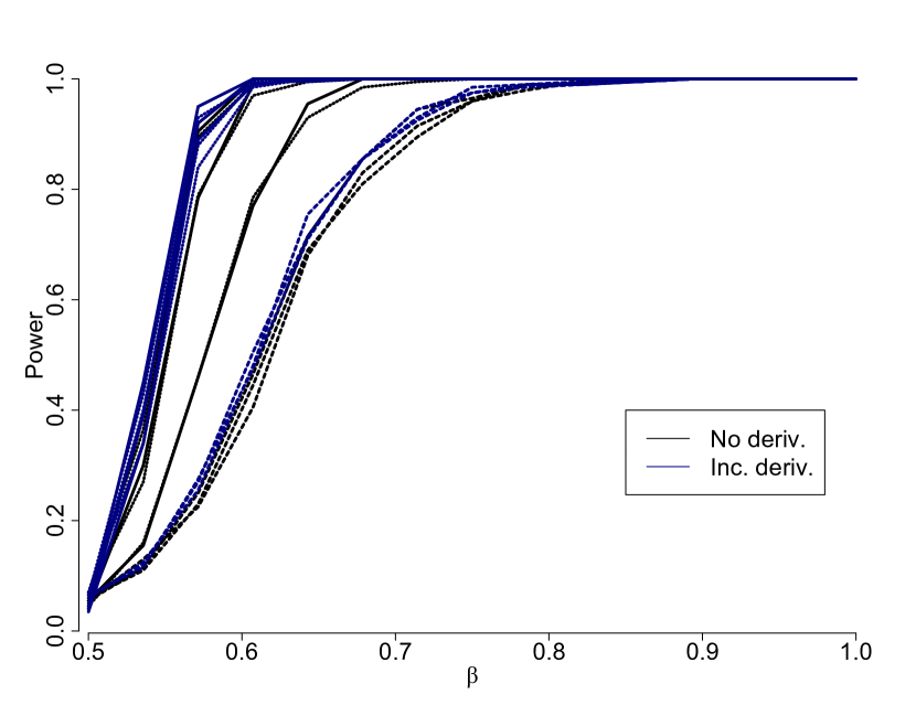
Figure 22: *

(a)

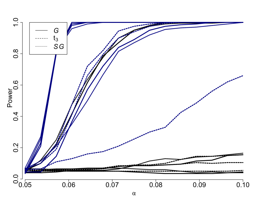
Figure 23: *

(b)

Figure 24: Comparison of the FKWC methods with the derivatives to the FKWC methods without the derivatives under (a) magnitude changes and (b) shape changes.

$(d_{1},d_{2})$	(0,0)	(0.4,0)	(0.8,0)	(0,0.4)	(0,0.8)	(0.4,0.4)
$\operatorname{MFHD}$	0.08	0.59	0.98	0.54	0.94	0.97
$\operatorname{RPD}$	0.07	0.77	0.99	0.68	0.99	0.99
$\operatorname{LTR}$	0.09	0.70	0.98	0.57	0.97	0.98
$\operatorname{MFHD}^{\prime}$	0.10	0.98	1.00	0.98	1.00	1.00
$\operatorname{RPD}^{\prime}$	0.06	0.97	1.00	0.97	1.00	1.00
$\operatorname{LTR}^{\prime}$	0.09	0.76	0.99	0.66	0.99	0.99

Table 3: Table of empirical powers at the $5\%$ level of significance for the AMOC FKWC test under the functional autoregressive model discussed in the simulation study of (Sharipov and Wendler, , 2020).

References

• Anderson and Miller, (1990) Anderson, R. J. and Miller, G. L. (1990). A simple randomized parallel algorithm for list-ranking. Information Processing Letters, 33(5):269–273.
• Aston et al., (2017) Aston, J. A. D., Pigoli, D., and Tavakoli, S. (2017). Tests for separability in nonparametric covariance operators of random surfaces. The Annals of Statistics, 45(4):1431–1461.
• Aue et al., (2018) Aue, A., Rice, G., and Sönmez, O. (2018). Structural break analysis for spectrum and trace of covariance operators. Technical report.
• Billingsley, (1968) Billingsley, P. (1968). Convergence of probability measures. Wiley, New York, first edition.
• Cerovecki et al., (2019) Cerovecki, C., Francq, C., Hörmann, S., and Zakoïan, J.-M. (2019). Functional GARCH models: The quasi-likelihood approach and its applications. Journal of Econometrics, 209(2):353 – 375.
• Chenouri et al., (2020) Chenouri, S., Mozaffari, A., and Rice, G. (2020). Robust multivariate change point analysis based on data depth. Canadian Journal of Statistics, 48(3):417–446.
• Claeskens et al., (2014) Claeskens, G., Hubert, M., Slaets, L., and Vakili, K. (2014). Multivariate functional halfspace depth. Journal of the American Statistical Association, 109:411–423.
• Cuevas et al., (2007) Cuevas, A., Febrero, M., and Fraiman, R. (2007). Robust estimation and classification for functional data via projection-based depth notions. Computational Statistics, 22:481–496.
• Dette and Kokot, (2020) Dette, H. and Kokot, K. (2020). Detecting relevant differences in the covariance operators of functional time series – a sup-norm approach. Technical report.
• Dette et al., (2020) Dette, H., Kokot, K., and Volgushev, S. (2020). Testing relevant hypotheses in functional time series via self-normalization. Journal of the Royal Statistical Society: Series B (Statistical Methodology), 82(3):629–660.
• Dette and Kutta, (2019) Dette, H. and Kutta, T. (2019). Detecting structural breaks in eigensystems of functional time series. Technical report.
• Feiner, (2019) Feiner, L. (2019). Twitter shares surge after earnings report shows growth in daily users. www.cnbc.com.
• Fraiman and Muniz, (2001) Fraiman, R. and Muniz, G. (2001). Trimmed means for functional data. Test, 10(2):419–440.
• Gijbels and Nagy, (2017) Gijbels, I. and Nagy, S. (2017). On a general definition of depth for functional data. Statistical Science, 32(4):630–639.
• Han, (2018) Han, F. (2018). An Exponential Inequality for U-Statistics Under Mixing Conditions. Journal of Theoretical Probability, 31(1):556–578.
• Harris, (2020) Harris, T. (2020). fmci. https://github.com/trevor-harris/fmci.
• Harris et al., (2021) Harris, T., Li, B., and Tucker, J. D. (2021). Scalable Multiple Changepoint Detection for Functional Data Sequences. Technical report.
• Hoeffding, (1963) Hoeffding, W. (1963). Probability inequalities for sums of bounded random variables. Journal of the American Statistical Association, 58(301):13–30.
• Hoffmann-Jørgensen, (2016) Hoffmann-Jørgensen, J. (2016). Maximal Inequalities for Dependent Random Variables. pages 61–104. Birkhäuser, Cham.
• Hubert et al., (2012) Hubert, M., Claeskens, G., Ketelaere, B. D., and Vakili, K. (2012). A new depth-based approach for detecting outlying curves. In Proceedings of COMPSTAT 2012, pages 329–340.
• Jarušková, (2013) Jarušková, D. (2013). Testing for a change in covariance operator. Journal of Statistical Planning and Inference, 143(9):1500–1511.
• Jiao et al., (2020) Jiao, S., Frostig, R. D., and Ombao, H. (2020). Break Point Detection for Functional Covariance. Technical report.
• Killick et al., (2012) Killick, R., Fearnhead, P., and Eckley, I. A. (2012). Optimal detection of changepoints with a linear computational cost. Journal of the American Statistical Association, 107(500):1590–1598.
• Nagy and Ferraty, (2019) Nagy, S. and Ferraty, F. (2019). Data depth for measurable noisy random functions. Journal of Multivariate Analysis, 170:95–114.
• Pitcan, (2017) Pitcan, Y. (2017). A Note on Concentration Inequalities for U-Statistics. arXiv e-prints, page arXiv:1712.06160.
• Pruss, (1998) Pruss, A. R. (1998). A Maximal Inequality for Partial Sums of Finite Exchangeable Sequences of Random Variables. Technical Report 6.
• Ramsay and Silverman, (2005) Ramsay, J. O. and Silverman, B. W. (2005). Functional Data Analysis. Springer Series in Statistics. Springer New York, New York, NY.
• Ramsay, (2021) Ramsay, K. (2021). FKWC_Changepoint. https://github.com/12ramsake/FKWC_Changepoint.
• Ramsay and Chenouri, (2020) Ramsay, K. and Chenouri, S. (2020). Robust, multiple change-point detection for covariance matrices using data depth. arXiv e-prints, page arXiv:2011.09558.
• Ramsay and Chenouri, (2021) Ramsay, K. and Chenouri, S. (2021). Robust nonparametric hypothesis tests for differences in the covariance structure of functional data. arXiv e-prints, page arXiv:2106.10173.
• Serfling and Wijesuriya, (2017) Serfling, R. and Wijesuriya, U. (2017). Depth-based nonparametric description of functional data, with emphasis on use of spatial depth. Computational Statistics & Data Analysis, 105:24–45.
• Sharipov and Wendler, (2020) Sharipov, O. S. and Wendler, M. (2020). Bootstrapping covariance operators of functional time series. Journal of Nonparametric Statistics, 32(3):648–666.
• Slaets, (2011) Slaets, L. (2011). Analyzing Phase and Amplitude Variation of Functional Data. PhD thesis, KU Leuven, Faculty of Business and Economics.
• Stoehr et al., (2019) Stoehr, C., Aston, J. A. D., and Kirch, C. (2019). Detecting changes in the covariance structure of functional time series with application to fMRI data. Technical report.
• Tukey, (1974) Tukey, J. W. (1974). Mathematics and the picturing of data. In Proceedings of the International Congress of Mathematicians.
• Yu and Chen, (2017) Yu, M. and Chen, X. (2017). Finite sample change point inference and identification for high-dimensional mean vectors. arXiv e-prints, page arXiv:1711.08747.