Universal minimal cost of coherent biochemical oscillations

Abstract

Biochemical clocks are essential for virtually all living systems. A biochemical clock that is isolated from an external periodic signal and subjected to fluctuations can oscillate coherently only for a finite number of oscillations. Furthermore, such an autonomous clock can oscillate only if it consumes free energy. What is the minimum amount of free energy consumption required for a certain number of coherent oscillations? We conjecture a universal bound that answers this question. A system that oscillates coherently for $\mathcal{N}$ oscillations has a minimal free energy cost per oscillation of $4\pi^{2}\mathcal{N}k_{B}T$. Our bound is valid for general finite Markov processes, is conjectured based on extensive numerical evidence, is illustrated with numerical simulations of a known model for a biochemical oscillator, and applies to existing experimental data.

Biological rhythms Novák and Tyson (2008); Goldbeter (2008); Ferrell et al. (2011) are essential for the proper operation of living systems ranging from bacteria to mammals. The most prominent biological oscillations are circadian rhythms that take 24 hours, but the period of biological rhythms has a wide range. One of the best understood circadian oscillators is KaiC, a protein that regulates the circadian clock of Cyanobacteria Nakajima et al. (2005); Dong and Golden (2008); Paijmans et al. (2017). In the presence of ATP and a few other molecules, KaiC molecules form a finite system of chemical reactions that produces circadian oscillations that can be observed in the laboratory. Another example of a finite system of chemical reactions that produces oscillations are synthetically engineered genetic circuits Potvin-Trottier et al. (2016).

In this context, consider an autonomous biochemical system composed of a finite number of molecules that oscillates. Fluctuations will eventually destroy the precision of the oscillations, i.e., if we consider different realizations of this biochemical system, they will dephase after some time. The quantity that characterizes the precision is the number of coherent oscillations $\mathcal{N}$ Barkai and Leibler (2000); Gaspard (2002); Gonze and Goldbeter (2006); Morelli and Jülicher (2007); Risau-Gusman, S. and Abramson, G. (2007); d'Eysmond et al. (2013), which is the decay time divided by the period of oscillation, as observed in a time-correlation function. In other words, if we isolate a biochemical clock in a “dark room”, i.e., without any external periodic stimuli, $\mathcal{N}$ roughly gives the number of oscillations for which the clock will still function properly.

A biochemical clock consumes free energy, in the form of ATP hydrolysis, or some other chemical fuel. A fundamental question then is: What is the minimal cost to sustain a biochemical oscillator with a precision quantified by $\mathcal{N}$? This cost can be characterized by the entropy production of stochastic thermodynamics Seifert (2012).

Two studies quite related to this question are the following. First, in Cao et al. (2015), the relation between the uncertainty in the period of oscillation, a quantity related to the number of coherent oscillations $\mathcal{N}$, and the entropy production was analyzed for several models. It was found that this uncertainty decreases linearly with the entropy production. Second, in Barato and Seifert (2017), a thermodynamic bound on $\mathcal{N}$ has been conjectured. This bound is expressed in terms of the thermodynamic affinity that drives the system out of equilibrium. This thermodynamic affinity does not suffice to know the free energy the system dissipates, which is quantified by the entropy production that additionally depends on detailed kinetic parameters.

Several works have addressed the relation between biochemical oscillations and stochastic thermodynamics Qian and Qian (2000); Nguyen et al. (2018); Fei et al. (2018); Wierenga et al. (2018); Marsland et al. (2019); Zhang et al. (2020); del Junco and Vaikuntanathan (2020a, b); Fritz et al. (2020). More generally, the relation between entropy production and precision of some kind has been a quite active area in the last 10 years in biophysics Qian (2007); Lan et al. (2012); Mehta and Schwab (2012); De Palo and Endres (2013); Skoge et al. (2013); Lang et al. (2014); Govern and ten Wolde (2014); Barato et al. (2014); Sartori et al. (2014); Hartich et al. (2015); Bo et al. (2015); Ito and Sagawa (2015); McGrath et al. (2017); Chiuchiú et al. (2019); Rana and Barato (2020); Seara et al. (2021).

In spite of all this research, the fundamental question raised above has remained unanswered. In this paper, we find that the number of coherent oscillations $\mathcal{N}$ has the minimal cost

$$\Delta S\geq 4\pi^{2}\mathcal{N},$$ (1)

where $\Delta S$ is the average entropy production per oscillation. For instance, a biochemical oscillator with $10$ coherent oscillations must dissipate at least approximately $395k_{B}T$ per oscillation, where $k_{B}$ is Boltzmann’s constant and $T$ is the temperature. This bound is independent of any details of the biochemical system. In fact, this bound can be violated only for $\mathcal{N}<(2\pi)^{-1}$, which amounts to a vanishing, practically undetectable, number of coherent oscillations. Our main result in Eq. (1) is a conjecture based on extensive numerical evidence.

A prominent relation in stochastic thermodynamics superficially related to our result is the thermodynamic uncertainty relation Barato and Seifert (2015). This relation establishes the minimal universal cost, as quantified by entropy production, related to the uncertainty of any thermodynamic current. Much work on the thermodynamic uncertainty relation has been done since its discovery Gingrich et al. (2016); Pietzonka et al. (2016); Nguyen and Vaikuntanathan (2016); Pietzonka and Seifert (2018); Polettini et al. (2016); Tsobgni Nyawo and Touchette (2016); Guioth and Lacoste (2016); Pietzonka et al. (2017); Horowitz and Gingrich (2017); Pigolotti et al. (2017); Proesmans and den Broeck (2017); Maes (2017); Hyeon and Hwang (2017); Bisker et al. (2017); Brandner et al. (2018); Nardini and Touchette (2018); Chiuchiù and Pigolotti (2018); Barato et al. (2018); Dechant and Sasa (2018); Carollo et al. (2019); Liu and Segal (2019); Guarnieri et al. (2019); Koyuk and Seifert (2020); Ito and Dechant (2020); Hasegawa (2021). In particular, the relation between the uncertainty of a thermodynamic current and the number of coherent oscillations has been analyzed in Nguyen et al. (2018). As shown in this reference the precision of biochemical oscillations is not well quantified by the uncertainty of a thermodynamic current. Hence, the uncertainty of a thermodynamic current is a different mathematical object and it has a different physical interpretation as a quantifier of precision. From the perspective of stochastic thermodynamics, the question we answer in this letter can be asked as follows. What is the minimal cost of the number of coherent oscillations as they are visible in time-correlation functions? Whereas the question answered by the thermodynamic uncertainty relation is: What is the minimal cost of precision of a thermodynamic current? The bound conjectured in Eq. (1) has the same degree of universality of the thermodynamic uncertainty relation first conjectured in Barato and Seifert (2015).

We consider continuous-time Markov processes with a finite number of states $\Omega$. The transition rate from state $i$ to state $j$ is denoted $k_{ij}$. The time evolution of the probability to be in state $i$ at time $t$, denoted $P_{i}(t)$, is determined by the master equation

$$\frac{d}{dt}P_{i}(t)=\sum_{j}\left[P_{j}(t)k_{ji}-P_{i}(t)k_{ij}\right].$$ (2)

In matrix form this equation can be written as $\frac{d}{dt}\mathbf{P}(t)=\mathbf{L}\mathbf{P}(t)$, where $\mathbf{P}(t)=\{P_{1}(t),P_{2}(t),\ldots,P_{\Omega}(t)\}^{T}$ and

$$\mathbf{L}_{ij}\equiv k_{ji}-\delta_{i,j}\sum_{l}k_{il}$$ (3)

is the stochastic matrix. We assume that if $k_{ij}\neq 0$ then $k_{ji}\neq 0$. Such Markov processes are an appropriate mathematical framework to describe a system of chemical reactions.

The long-time stationary distribution is denoted by $P_{i}$. This distribution is the right eigenvector associated with the eigenvalue of $L$ with largest real part, which is $0$. The stationary rate of entropy production from stochastic thermodynamics is Seifert (2012)

$$\sigma\equiv\sum_{ij}P_{i}k_{ij}\ln\frac{k_{ij}}{k_{ji}}\geq 0.$$ (4)

The rate of entropy production vanishes only if the steady state is an equilibrium one. An equilibrium steady state fulfills the detailed balance relation $P_{i}k_{ij}=P_{j}k_{ji}$ for all pairs $i,j$.

Consider a system of chemical reactions that generates oscillations and is well described as a Markov process. The concentration of an oscillating chemical species can generically be written as a time-correlation function, which is a linear combination of the time-dependent probabilities $P_{i}(t)$ that are obtained as the solution of Eq. (2). Therefore, the period and decay time of the biochemical oscillations are quantified by the first non-trivial eigenvalue of $\mathbf{L}$, i.e., the non-zero eigenvalue with the smallest modulus of its real part Barato and Seifert (2017).

This eigenvalue is written as $\lambda=-\lambda_{R}\pm i\lambda_{I}$. The decay time is $\lambda_{R}^{-1}$ and the period of oscillation is $2\pi\lambda_{I}^{-1}$. The number of coherent oscillations is given by

$$\mathcal{N}\equiv\frac{1}{2\pi}\frac{\lambda_{I}}{\lambda_{R}}.$$ (5)

This quantity $\mathcal{N}$ that quantifies the precision of the oscillations is dimensionless, while the entropy production rate $\sigma$ that quantifies the cost has dimension of $t^{-1}$. In order to make the cost dimensionless we consider the entropy produced in one period of oscillation

$$\Delta S\equiv\sigma\times(2\pi\lambda_{I}^{-1}).$$ (6)

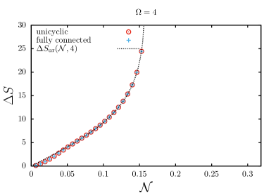
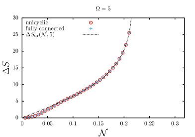
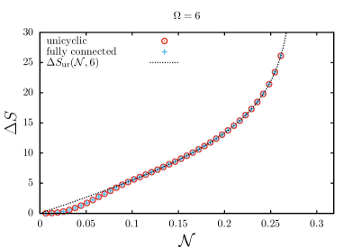
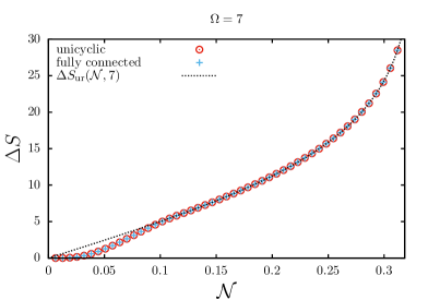
Figure 1: (Color online) Minimal cost per period $\Delta S$ as a function of the number of coherent oscillations $\mathcal{N}$, obtained from numerical minimization for fully connected networks and for unicylic networks. Both are compared to the analytical form for uniform rates in Eq. (10).

Unicyclic networks Derrida (1983) play a central role in our calculations. For these networks, transition rates from state $i$ are nonzero only to its two nearest neighbors $i+1$ and $i-1$. Unicyclic networks have periodic boundary conditions, for $i=\Omega$ the right neighbor is $i+1=1$ and for $i=1$ the left neighbor is $i-1=\Omega$. The transition rate from $i$ to $i+1$ is denoted by $k_{i,i+1}$. The affinity of a unicyclic network is defined as

$$A\equiv\ln\left(\prod_{i=1}^{\Omega}\frac{k_{i,i+1}}{k_{i,i-1}}\right).$$ (7)

The affinity $A$ is the thermodynamic force that drives the system out of equilibrium. The system reaches a stationary equilibrium state only if $A=0$.

Consider a unicyclic network with affinity $A$ and number of states $\Omega$. Uniform rates are given by $k_{i,i+1}=k\textrm{e}^{A/\Omega}$ and $k_{i,i-1}=k$, for all $i$, where $k>0$ is a constant that sets the time scale of the rates. For such uniform rates, from the fact that the stationary probability of a random walk in a circle is uniform and from Eq. (4), we obtain

$$\Delta S_{\textrm{ur}}=\frac{2\pi A}{\Omega\sin(2\pi/\Omega)}.$$ (8)

From the calculation of the first non-trivial eigenvalue and Eq. (5), we obtain

$$\mathcal{N}=\frac{1}{2\pi}\cot\left(\frac{\pi}{\Omega}\right)\tanh\left(\frac{A}{2\Omega}\right).$$ (9)

By eliminating the affinity $A$ we obtain,

$$\Delta S_{\textrm{ur}}(\mathcal{N},\Omega)=\frac{4\pi}{\sin(2\pi/\Omega)}\textrm{arctanh}[2\pi\mathcal{N}\tan(\pi/\Omega)]\geq 4\pi^{2}\mathcal{N},$$ (10)

where the inequality comes from the fact that $\Delta S_{\textrm{ur}}(\mathcal{N},\Omega)$ is a decreasing function of $\Omega$ and $\lim_{\Omega\to\infty}\Delta S_{\textrm{ur}}(\mathcal{N},\Omega)=4\pi^{2}\mathcal{N}$. This analytical expression will be important for the derivation of our main result.

Let us now consider the procedure of obtaining $\Delta S$ as a function of $\mathcal{N}$. Both quantities depend on the transition rates. Numerically we can impose the constraint that $\mathcal{N}$ is fixed and minimize $\Delta S$. Technically this minimization is done with the Python routine scipy.optimize.minimize. We have performed this minimization for $\Omega=4,5,6,7$, for both fully connected networks, which include all possible networks since some of the rates can be set to zero, and for the more restricted case of unicyclic networks. As shown in Fig. 1, both procedures lead to the same minimum. For large enough $\mathcal{N}$ the minimum has the functional form that is obtained for the case of uniform rates in Eq. (10). For small $\mathcal{N}$ the numerical minimum goes below the expression in Eq. (10). The value of $\mathcal{N}$ for which the minimum deviates from the expression in Eq. (10) gets larger for larger system size $\Omega$. Therefore, our numerical results show that the minimum of $\Delta S$ for fixed $\mathcal{N}$ is given by the numerical minimization of unicyclic networks.

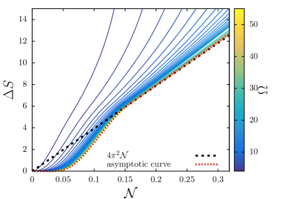
Figure 2: (Color online) Numerical minimization for unicycle networks from $\Omega=4$ up to $\Omega=55$. The red dashed line is the asymptotic curve $\Omega\to\infty$ obtained with numerical interpolation.

Restricting to unicyclic networks allows us to calculate the numerical minimal $\Delta S$ for fixed $\mathcal{N}$ from $\Omega=4$ up to $\Omega=55$, as shown in Fig 2. From these curves we obtain the curve corresponding to the limit $\Omega\to\infty$. In particular, for fixed $\mathcal{N}$ we fit a function of the type $\Delta S(\Omega)=a*\Omega^{b}+c$, where the parameter $c$ provides the limiting value of $\Delta S$. This limit curve gives our main result in Eq. (1). For $\mathcal{N}\geq(2\pi)^{-1}$, the minimal cost $\Delta S$ for a certain number of coherent oscillations $\mathcal{N}$ is given by the $\Omega\to\infty$ function for uniform rates in Eq. (10). For $\mathcal{N}<(2\pi)^{-1}$, the minimum $\Delta S$ goes below $4\pi^{2}\mathcal{N}$ and its form is given by the numerically determined asymptotic curve in Fig. 2. Since, a system with $\mathcal{N}=(2\pi)^{-1}$ will not show any visible oscillation, for any biochemical oscillator with a reasonable number of coherent oscillations the bound in Eq. (10) establishes the minimal universal cost of coherent oscillations. However, this small $\mathcal{N}$ region, for which uniform rates do not minimize $\Delta S$, is an important mathematical feature of the bound that should be taken into account in future analytical studies.

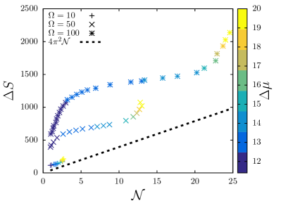
Figure 3: (Color online) Illustration of the bound with a model for a system of KaiC molecules. Data for $\mathcal{N}$ is taken from Nguyen et al. (2018). The parameter $\Omega$ represents the number of KaiC molecules and the parameter $\Delta\mu$ is the free energy of one ATP hydrolysis.

In order to illustrate our bound we compare Eq. (1) to an established model for a system of KaiC molecules in Fig. 3. The data for $\mathcal{N}$ are taken from Fig. 11 in Ref. Nguyen et al. (2018). The definition of the model with the exact parameters are given in Sec. II C of this reference. The parameter $\Omega$, following the notation of this reference, is the number of KaiC molecules (and not exactly the total number of states used in our calculations above). The parameter $\Delta\mu$ is the free energy of one ATP hydrolysis, i.e., the affinity that drives the system out of equilibrium. Each KaiC molecule has 6 phosphorylation sites and the quantity that oscillates is the phosphorylation level of the system of KaiC molecules.

The cost $\Delta S$ for this more complex model stays above the lower bound conjectured here. For larger system sizes $\Omega$, $\Delta S$ is substantially above the bound. Since both $\mathcal{N}$ and $\Delta S$ increase linearly with system size, it is not clear whether this observation is generic. Even for larger system sizes, the exact $\Delta S$ is not more than one order of magnitude above the bound. This particular example shows that a reasonably realistic model can operate close to the bound.

Our bounds can be seen from a different perspective. Consider a biochemical oscillator for which we can measure a time-correlation function of an oscillating chemical concentration. From this correlation function, $\mathcal{N}$ can be evaluated, which together with Eq. (1) implies a lower bound on the amount of free energy consumption per period. This lower bound is independent of any knowledge about the molecular details of the biochemical oscillator. In fact, our results can be applied to extant experimental data. As an example, we consider the repressilator from Ref. Potvin-Trottier et al. (2016). We have estimated the number of coherent oscillations from the plots of the correlation function shown in Fig. 1e and Fig. 2c in this reference, which correspond to two different situations. For the first case we estimate $\mathcal{N}\simeq 0.57$, which implies a minimum free energy cost per period of $22.5k_{B}T$. For the second case we estimate $\mathcal{N}\simeq 1.42$, which implies a minimum free energy cost per period of $56.0k_{B}T$.

The present results are related to the bound conjectured in Barato and Seifert (2017). For simplicity, we will restrict the discussion to the case of unicyclic networks. In that reference it was shown that for a network with affinity $A$ and number of states $\Omega$

$$\mathcal{N}\leq\frac{1}{2\pi}\cot(\pi/\Omega)\tanh\left(\frac{A}{2\Omega}\right)\leq\frac{1}{4\pi^{2}}A,$$ (11)

where the second inequality corresponds to the limit $\Omega\to\infty$. Even though this bound and our result in Eq. (1) look similar, they are mathematically and physically different. Mathematically, the bound in Eq. (11) was obtained by maximizing $\mathcal{N}$ for fixed $A$ and $\Omega$ in Barato and Seifert (2017). For this quantity, the maximum is reached for uniform rates, independent of the value of $\mathcal{N}$. Our bound in Eq. (1) can be obtained by maximizing the same function $\mathcal{N}$ but with the very different constraint that the entropy production per oscillation $\Delta S$ is fixed, which is analogous to minimize $\Delta S$ with the constraint that $\mathcal{N}$ is fixed. Fixing $\Delta S$ is a much more complicated constraint due to its complex dependence on the transition rates. The present bound also displays the intricate nonlinear behavior for small $\mathcal{N}$, in this regime $\mathcal{N}$ is not maximized for the case of uniform rates and Eq. (1) is violated. The factor $4\pi^{2}$ shows up in both bounds since both are related to the limit $\Omega\to\infty$ for the case of uniform rates.

The physical difference between both bounds comes from the physical difference between $A$ and $\Delta S$. The affinity $A$ is independent of kinetic parameters and does not provide any quantitative information about free energy cost. The affinity $A$ depends on thermodynamic parameters such as ATP concentration and temperature. In contrast, entropy production per oscillation $\Delta S$ is a much more complex quantity. It depends on model specific kinetic parameters and quantifies the free energy cost per oscillation.

In conclusion, a biochemical oscillator can only show a certain number of coherent oscillations if it dissipates a minimal amount of free energy, as dictated by Eq. (1). This bound constitutes a new universal law for biochemical oscillators. It is also an inference tool: measurement of the decay time and period of oscillation of a biochemical clock leads to a lower bound on its free energy consumption.

From the perspective of stochastic thermodynamics, fluctuations cannot take any form but are bounded by universal relations. Two of the most prominent such relation are the fluctuation theorem and the thermodynamic uncertainty relation. Our bound adds one more relation to the list, the number of coherent oscillations as visible in a time correlation function is bounded by the entropy production.

The main result presented here is a conjecture based on numerical evidence, a full mathematical proof remains an open problem. From a broad perspective, it is interesting to ask whether the present bound and the thermodynamic uncertainty relation can be derived from a deeper master relation. Concerning applications, our universal bound could be used to, inter alia, infer free energy dissipation and to optimize the number of coherent oscillations with a given free energy budget. Moreover, to investigate whether real biochemical clocks operate close to the bound is an interesting question for future work.

References

- Novák and Tyson (2008) B. Novák and J. J. Tyson, Nature Rev. Mol. Cell Biol. 9, 981 (2008).
- Goldbeter (2008) A. Goldbeter, Curr. Biol. 18, R751 (2008).
- Ferrell et al. (2011) J. E. Ferrell, T. Y.-C. Tsai, and Q. Yang, Cell 144, 874 (2011).
- Nakajima et al. (2005) M. Nakajima, K. Imai, H. Ito, T. Nishiwaki, Y. Murayama, H. Iwasaki, T. Oyama, and T. Kondo, Science 308, 414 (2005).
- Dong and Golden (2008) G. Dong and S. S. Golden, Curr. Opin. Microbiol. 11, 541 (2008).
- Paijmans et al. (2017) J. Paijmans, D. K. Lubensky, and P. R. Ten Wolde, Biophys J. 113, 157 (2017).
- Potvin-Trottier et al. (2016) L. Potvin-Trottier, N. D. Lord, G. Vinnicombe, and J. Paulsson, Nature 538, 514 (2016).
- Barkai and Leibler (2000) N. Barkai and S. Leibler, Nature 403, 267 (2000).
- Gaspard (2002) P. Gaspard, J. Chem. Phys. 117, 8905 (2002).
- Gonze and Goldbeter (2006) D. Gonze and A. Goldbeter, Chaos 16, 026110 (2006).
- Morelli and Jülicher (2007) L. G. Morelli and F. Jülicher, Phys. Rev. Lett. 98, 228101 (2007).
- Risau-Gusman, S. and Abramson, G. (2007) Risau-Gusman, S. and Abramson, G., Eur. Phys. J. B 60, 515 (2007).
- d'Eysmond et al. (2013) T. d'Eysmond, A. D. Simone, and F. Naef, Physical Biology 10, 056005 (2013).
- Seifert (2012) U. Seifert, Rep. Prog. Phys. 75, 126001 (2012).
- Cao et al. (2015) Y. Cao, H. Wang, Q. Ouyang, and Y. Tu, Nat. Phys. 11, 772 (2015).
- Barato and Seifert (2017) A. C. Barato and U. Seifert, Phys. Rev. E 95, 062409 (2017).
- Qian and Qian (2000) H. Qian and M. Qian, Phys. Rev. Lett. 84, 2271 (2000).
- Nguyen et al. (2018) B. Nguyen, U. Seifert, and A. C. Barato, J. Chem. Phys. 149, 045101 (2018).
- Fei et al. (2018) C. Fei, Y. Cao, Q. Ouyang, and Y. Tu, Nat. Commun. 9, 1434 (2018).
- Wierenga et al. (2018) H. Wierenga, P. R. ten Wolde, and N. B. Becker, Phys. Rev. E 97, 042404 (2018).
- Marsland et al. (2019) R. Marsland, W. Cui, and J. M. Horowitz, J. R. Soc. Interface 16, 20190098 (2019).
- Zhang et al. (2020) D. Zhang, Y. Cao, Q. Ouyang, and Y. Tu, Nat. Phys. 16, 95 (2020).
- del Junco and Vaikuntanathan (2020a) C. del Junco and S. Vaikuntanathan, Phys. Rev. E 101, 012410 (2020a).
- del Junco and Vaikuntanathan (2020b) C. del Junco and S. Vaikuntanathan, J. Chem. Phys. 152, 055101 (2020b).
- Fritz et al. (2020) J. H. Fritz, B. Nguyen, and U. Seifert, J. Chem. Phys. 152, 235101 (2020).
- Qian (2007) H. Qian, Annu. Rev. Phys. Chem. 58, 113 (2007).
- Lan et al. (2012) G. Lan, P. Sartori, S. Neumann, V. Sourjik, and Y. Tu, Nature Phys. 8, 422 (2012).
- Mehta and Schwab (2012) P. Mehta and D. J. Schwab, Proc. Natl. Acad. Sci. U.S.A. 109, 17978 (2012).
- De Palo and Endres (2013) G. De Palo and R. G. Endres, PLoS Comput. Biol. 9, e1003300 (2013).
- Skoge et al. (2013) M. Skoge, S. Naqvi, Y. Meir, and N. S. Wingreen, Phys. Rev. Lett. 110, 248102 (2013).
- Lang et al. (2014) A. H. Lang, C. K. Fisher, T. Mora, and P. Mehta, Phys. Rev. Lett. 113, 148103 (2014).
- Govern and ten Wolde (2014) C. C. Govern and P. R. ten Wolde, Phys. Rev. Lett. 113, 258102 (2014).
- Barato et al. (2014) A. C. Barato, D. Hartich, and U. Seifert, New J. Phys. 16, 103024 (2014).
- Sartori et al. (2014) P. Sartori, L. Granger, C. F. Lee, and J. M. Horowitz, PLoS Comput. Biol. 10, e1003974 (2014).
- Hartich et al. (2015) D. Hartich, A. C. Barato, and U. Seifert, New J. Phys. 17, 055026 (2015).
- Bo et al. (2015) S. Bo, M. Del Giudice, and A. Celani, J. Stat. Mech.: Theor. Exp. 2015, P01014 (2015).
- Ito and Sagawa (2015) S. Ito and T. Sagawa, Nat. Commun. 6, 7498 (2015).
- McGrath et al. (2017) T. McGrath, N. S. Jones, P. R. ten Wolde, and T. E. Ouldridge, Phys. Rev. Lett. 118, 028101 (2017).
- Chiuchiú et al. (2019) D. Chiuchiú, Y. Tu, and S. Pigolotti, Phys. Rev. Lett. 123, 038101 (2019).
- Rana and Barato (2020) S. Rana and A. C. Barato, Phys. Rev. E 102, 032135 (2020).
- Seara et al. (2021) D. S. Seara, B. B. Machta, and M. P. Murrell, Nat. Commun. 12, 1 (2021).
- Barato and Seifert (2015) A. C. Barato and U. Seifert, Phys. Rev. Lett. 114, 158101 (2015).
- Gingrich et al. (2016) T. R. Gingrich, J. M. Horowitz, N. Perunov, and J. L. England, Phys. Rev. Lett. 116, 120601 (2016).
- Pietzonka et al. (2016) P. Pietzonka, A. C. Barato, and U. Seifert, Phys. Rev. E 93, 052145 (2016).
- Nguyen and Vaikuntanathan (2016) M. Nguyen and S. Vaikuntanathan, PNAS 113, 14231 (2016).
- Pietzonka and Seifert (2018) P. Pietzonka and U. Seifert, Phys. Rev. Lett. 120, 190602 (2018).
- Polettini et al. (2016) M. Polettini, A. Lazarescu, and M. Esposito, Phys. Rev. E 94, 052104 (2016).
- Tsobgni Nyawo and Touchette (2016) P. Tsobgni Nyawo and H. Touchette, Phys. Rev. E 94, 032101 (2016).
- Guioth and Lacoste (2016) J. Guioth and D. Lacoste, EPL 115, 60007 (2016).
- Pietzonka et al. (2017) P. Pietzonka, F. Ritort, and U. Seifert, Phys. Rev. E 96, 012101 (2017).
- Horowitz and Gingrich (2017) J. M. Horowitz and T. R. Gingrich, Phys. Rev. E 96, 020103 (2017).
- Pigolotti et al. (2017) S. Pigolotti, I. Neri, E. Roldán, and F. Jülicher, Phys. Rev. Lett. 119, 140604 (2017).
- Proesmans and den Broeck (2017) K. Proesmans and C. V. den Broeck, EPL 119, 20001 (2017).
- Maes (2017) C. Maes, Phys. Rev. Lett. 119, 160601 (2017).
- Hyeon and Hwang (2017) C. Hyeon and W. Hwang, Phys. Rev. E 96, 012156 (2017).
- Bisker et al. (2017) G. Bisker, M. Polettini, T. R. Gingrich, and J. M. Horowitz, J. Stat. Mech.: Theor. Exp. 2017, 093210 (2017).
- Brandner et al. (2018) K. Brandner, T. Hanazato, and K. Saito, Phys. Rev. Lett. 120, 090601 (2018).
- Nardini and Touchette (2018) C. Nardini and H. Touchette, Eur. Phys. J. B 91, 16 (2018).
- Chiuchiù and Pigolotti (2018) D. Chiuchiù and S. Pigolotti, Phys. Rev. E 97, 032109 (2018).
- Barato et al. (2018) A. C. Barato, R. Chetrite, A. Faggionato, and D. Gabrielli, New J. Phys. 20, 103023 (2018).
- Dechant and Sasa (2018) A. Dechant and S.-i. Sasa, J. Stat. Mech.: Theor. Exp. 2018, 063209 (2018).
- Carollo et al. (2019) F. Carollo, R. L. Jack, and J. P. Garrahan, Phys. Rev. Lett. 122, 130605 (2019).
- Liu and Segal (2019) J. Liu and D. Segal, Phys. Rev. E 99, 062141 (2019).
- Guarnieri et al. (2019) G. Guarnieri, G. T. Landi, S. R. Clark, and J. Goold, Phys. Rev. Research 1, 033021 (2019).
- Koyuk and Seifert (2020) T. Koyuk and U. Seifert, Phys. Rev. Lett. 125, 260604 (2020).
- Ito and Dechant (2020) S. Ito and A. Dechant, Phys. Rev. X 10, 021056 (2020).
- Hasegawa (2021) Y. Hasegawa, Phys. Rev. Lett. 126, 010602 (2021).
- Derrida (1983) B. Derrida, J. Stat. Phys. 31, 433 (1983).