The Gardner problem and cycle slipping bifurcation for type 2 phase-locked loops

Abstract

In the present work, a second-order type 2 PLL with a piecewise-linear phase detector characteristic is analysed. An exact solution to the Gardner problem on the lock-in range is obtained for the considered model. The solution is based on a study of cycle slipping bifurcation and improves well-known engineering estimates.

1 Introduction

Phase-locked loops (PLLs) are nonlinear control systems which are designed to synchronize a voltage-controlled oscillator (VCO) signal with a reference one. PLLs have many applications in energy and robotic systems, satellite navigation, wireless and optical communications, cyber-physical systems Du & Swamy [2010]; Karimi-Ghartemani [2014]; Rosenkranz & Schaefer [2016]; Best et al. [2016]; Kaplan & Hegarty [2017]; Kuznetsov et al. [2020c]; Zelenskii et al. [2021]; Zelensky et al. [2021]; Kuznetsov et al. [2022]. Analog PLLs can be described by systems of nonlinear differential equations with periodic right-hand sides, which are also known as pendulum-like systems. In 1933, F. Tricomi was the first, who conducted nonlinear analysis Tricomi [1933] of the systems which are equivalent to the second-order PLLs with lag filters (see, e.g., Gardner [2005]). It was proven that the global stability of those systems is determined by separatrices of a saddle, which correspond to a heteroclinic bifurcation in the system. Further, bifurcations of the second-order PLLs with lead-lag filters and different nonlinear characteristics of phase detectors were studied in Andronov et al. [1937]; Kapranov [1956]; Belyustina [1959]; Gubar’ [1961]; Shakhtarin [1969].

PLL systems with lag and lead-lag loop filters can be classified as type 1 PLLs, because transfer functions of such filters do not have poles at the origin. In engineering practice, so-called type 2 PLLs, that have loop filters with exactly one pole at the origin, are most often used nowadays Gardner [2005]. The second-order type 2 analog PLLs are always globally stable (see, e.g., Kuznetsov et al. [2021a]), i.e., these PLLs acquire lock for any reference frequency. However, synchronization in the systems may take long time. In order to reduce the long acquisition time, the lock-in concept has been introduced. According to the concept, the locked PLL re-acquires a locked state without cycle slipping after an abrupt change of the reference frequency. The problem of estimation of the reference frequencies where the concept is held was posed by F. Gardner in his monograph Gardner [2005]. A rigorous approach to the Gardner problem and analytical estimates of the lock-in range were suggested in Kuznetsov et al. [2015, 2019b, 2021a, 2021c, 2021b].

The system where such abrupt reference frequency change occurs can be considered as a switching system. The Gardner problem requires to study cycle slipping bifurcation of the system when a trajectory, starting from an equilibrium of the system before the switch tends to an equilibrium of the system after the switch. This task is similar to the problem of the heteroclinic bifurcation estimation in type 1 PLL systems.

2 Mathematical Model and Stability Analysis

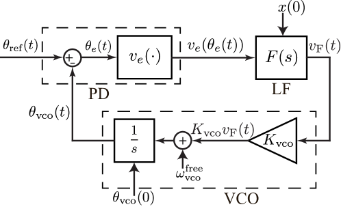
Figure 1: Baseband model of analog PLLs.

Consider analog PLL baseband model in Fig. 1 Gardner [2005]; Viterbi [1966]; Best [2007]; Leonov et al. [2012, 2015b]. Here $\theta_{\rm ref}(t)=\omega_{\rm ref}t+\theta_{\rm ref}(0)$ is a phase of the reference signal, a phase of the VCO is $\theta_{\rm vco}(t)$, $\theta_{e}(t)=\theta_{\rm ref}(t)-\theta_{\rm vco}(t)$ is a phase error. A phase detector (PD) generates a signal $v_{e}(\theta_{e}(t))$ where $v_{e}(\cdot)$ is a characteristic of the phase detector. In the present paper, a piecewise-linear PD characteristic, which is continuous and corresponds to square waveforms of the reference and the VCO signals, is considered:

$$v_{e}(\theta_{e})=\begin{cases}&k\theta_{e}-2\pi km,\qquad-\frac{1}{k}+2\pi m\leq\theta_{e}(t)<\frac{1}{k}+2\pi m,\\ &-\frac{1}{\pi-\frac{1}{k}}\theta_{e}+\frac{1}{\pi-\frac{1}{k}}(\pi+2\pi m),\qquad\frac{1}{k}+2\pi m\leq\theta_{e}(t)<-\frac{1}{k}+2\pi(m+1),\end{cases}$$ (1)

here $k>\frac{1}{\pi},\ m\in\mathbb{Z}$ (see Fig. 2).

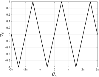
Figure 2: Triangular PD characteristic (piecewise-linear PD characteristic (1) with $k=\frac{2}{\pi}$).

The state of the loop filter is represented by $x(t)\in\mathbb{R}$ and the transfer function is

$$F(s)=\frac{1+s\tau_{2}}{s\tau_{1}},\quad\tau_{1}>0,\ \tau_{2}>0.$$

The output of the loop filter $v_{\rm F}(t)=\frac{1}{\tau_{1}}(x(t)+\tau_{2}v_{e}(\theta_{e}(t))$ is used to control the VCO frequency $\omega_{\rm vco}(t)$, which is proportional to the control voltage:

$$\omega_{\rm vco}(t)=\dot{\theta}_{\rm vco}(t)=\omega_{\rm vco}^{\rm free}+K_{\rm vco}v_{\rm F}(t)$$

where $K_{\rm vco}>0$ is a gain and $\omega_{\rm vco}^{\rm free}$ is a free-running frequency of the VCO.

The behavior of PLL baseband model in the state space is described by a second-order nonlinear ODE:

$$\dot{x}=v_{e}(\theta_{e}),$$ (2)

$$\dot{\theta}_{e}=\omega_{e}^{\rm free}-\frac{K_{\rm vco}}{\tau_{1}}\Big{(}x+\tau_{2}v_{e}(\theta_{e})\Big{)}$$

where $\omega_{e}^{\rm free}=\omega_{\rm ref}-\omega_{\rm vco}^{\rm free}$ is a frequency error and $v_{e}(\theta_{e})$ is defined in (1). It is usually supposed that the reference frequency (hence, $\omega_{e}^{\rm free}$ too) can be abruptly changed and that the synchronization occurs between those changes. Thus, existence of locked states, acquisition and transient processes after the reference frequency change are of interest.

2.1 Local stability analysis

The PLL baseband model in Fig. 1 is locked if the phase error $\theta_{e}(t)$ is constant. For the locked states of practically used PLLs, the loop filter state is constant too and, thus, the locked states of model in Fig. 1 correspond to the equilibria of model (2) Kuznetsov et al. [2015].

Definition 2.1.

Kuznetsov et al. [2015]; Leonov et al. [2015a]; Best et al. [2016] A hold-in range is the largest symmetric interval of frequency errors $|\omega_{e}^{\rm free}|$ such that an asymptotically stable equilibrium exists and varies continuously while $\omega_{e}^{\rm free}$ varies continuously within the interval.

Observe that system (2) is $2\pi$-periodic in $\theta_{e}$ and has an infinite number of equilibria $\left(\frac{\tau_{1}\omega_{e}^{\rm free}}{K_{\rm vco}},\ \pi m\right)$, $m\in\mathbb{Z}$. The characteristic polynomial of system (2) linearized at stationary states $\left(\frac{\tau_{1}\omega_{e}^{\rm free}}{K_{\rm vco}},\pi m\right)$ is

$$\chi(s)=s^{2}+\frac{K_{\rm vco}\tau_{2}}{\tau_{1}}v_{e}^{\prime}(\pi m)s+\frac{K_{\rm vco}}{\tau_{1}}v_{e}^{\prime}(\pi m).$$

The nonlinearity $v_{e}(\theta_{e})$ decreases $\left(v_{e}^{\prime}(\pi+2\pi m)=-\frac{1}{\pi-\frac{1}{k}}<0\right)$ for $\frac{1}{k}+2\pi m<\theta_{e}(t)<-\frac{1}{k}+2\pi(m+1)$, and equilibria $\left(\frac{\tau_{1}\omega_{e}^{\rm free}}{K_{\rm vco}},\pi+2\pi m\right)$ are saddles. The nonlinearity $v_{e}(\theta_{e})$ increases ($v_{e}^{\prime}(2\pi m)=k>0$) for $-\frac{1}{k}+2\pi m<\theta_{e}(t)<\frac{1}{k}+2\pi m$, and the equilibria $\left(\frac{\tau_{1}\omega_{e}^{\rm free}}{K_{\rm vco}},2\pi m\right)$ are asymptotically stable:

if $\frac{K_{\rm vco}\tau_{2}^{2}k}{\tau_{1}}>4$ then the equilibria $\left(\frac{\tau_{1}\omega_{e}^{\rm free}}{K_{\rm vco}},2\pi m\right)$ are asymptotically stable nodes,

if $\frac{K_{\rm vco}\tau_{2}^{2}k}{\tau_{1}}=4$ then the equilibria $\left(\frac{\tau_{1}\omega_{e}^{\rm free}}{K_{\rm vco}},2\pi m\right)$ are asymptotically stable degenerate nodes,

if $\frac{K_{\rm vco}\tau_{2}^{2}k}{\tau_{1}}<4$ then the equilibria $\left(\frac{\tau_{1}\omega_{e}^{\rm free}}{K_{\rm vco}},2\pi m\right)$ are asymptotically stable focuses. Since an asymptotically stable equilibrium exists for any frequency error $\omega_{e}^{\rm free}$, the hold-in range of model (2) is infinite for any loop parameters $K_{\rm vco}>0,\ \tau_{1}>0,\ \tau_{2}>0$.

2.2 Global stability analysis

Definition 2.2.

Kuznetsov et al. [2015]; Leonov et al. [2015a]; Best et al. [2016] A pull-in range is the largest symmetric interval of frequency errors $|\omega_{e}^{\rm free}|$ from the hold-in range such that an equilibrium is acquired for an arbitrary initial state.

In 1959, Andrew J. Viterbi applied the phase-plane analysis and stated that the second-order type 2 PLL models with sinusoidal PD characteristic have infinite (theoretically) hold-in and pull-in ranges for any loop parameters [Viterbi, 1959, p.12], Viterbi [1966]. However, his proof was incomplete (see, e.g. discussion in Alexandrov et al. [2015]). Later, Viterbi’s statement was rigorously proved using the direct Lyapunov method ideas Bakaev [1963]; Aleksandrov et al. [2016]; Kuznetsov et al. [2021a].

To analyse the pull-in range of system (2) with piecewise-linear PD characteristic, we apply the direct Lyapunov method and the corresponding theorem on global stability for the cylindrical phase space (see, e.g. Leonov & Kuznetsov [2014]; Kuznetsov et al. [2020b]). If there is a continuous function $V(x,\theta_{e}):\mathbb{R}^{n}\to\mathbb{R}$ such that

(i) $V(x,\theta_{e}+2\pi)=V(x,\theta_{e})\quad\forall x\in\mathbb{R}^{n-1},\forall\theta_{e}\in\mathbb{R}$;

(ii) for any solution $(x(t),\theta_{e}(t))$ of system (2) the function $V(x(t),\theta_{e}(t))$ is nonincreasing;

(iii) if $V(x(t),\theta_{e}(t))\equiv V(x(0),\theta_{e}(0))$, then $(x(t),\theta_{e}(t))\equiv~{}(x(0),\theta_{e}(0))$;

(iv) $V(x,\theta_{e})+\theta_{e}^{2}\to+\infty$ as $||x||+|\theta_{e}|\to+\infty$
then any trajectory of system (2) tends to an equilibrium (for brevity, we shall call such systems globally stable).

Consider the following Lyapunov function:

$$V(x,\theta_{e})=\frac{K_{\rm vco}}{2\tau_{1}}\left(x-\frac{\tau_{1}\omega_{e}^{\rm free}}{K_{\rm vco}}\right)^{2}+\int\limits_{0}^{\theta_{e}}v_{e}(\sigma)d\sigma.$$ (3)

Its derivative along the trajectories of system (2) is

$$\dot{V}(x,\theta_{e})=-\frac{K_{\rm vco}\tau_{2}}{\tau_{1}}v_{e}^{2}(\theta_{e})<0\quad\forall\theta_{e}\neq\pi m,\ m\in\mathbb{Z}.$$

Since the derivative along any solution other than stationary states is not identically zero, system (2) is globally stable for any $\omega_{e}^{\rm free}$ and, hence, the pull-in range is infinite.

In 1981, William F. Egan conjectured [Egan, 1981, p.176] that a higher-order type 2 PLL with an infinite hold-in range also has an infinite pull-in range, and supported it with some third-order PLL implementations (see also [Egan, 2007, p.161]). However, this conjecture is not valid in general and corresponding counterexamples were recently provided in Kuznetsov et al. [2021a].

Notice that a similar conjecture on the pull-in range for the second-order type 1 PLLs is known as the Kapranov conjecture Kapranov [1956], where it is supposed that the global stability of the corresponding model is determined by the birth of self-excited oscillations only, not hidden ones Leonov & Kuznetsov [2013]; Chen et al. [2017]. Discussions of counterexamples to the Kapranov conjecture can be found in Kuznetsov et al. [2017]; Kuznetsov [2020].

3 The lock-in range of second-order type 2 analog PLL with piecewise-linear PD characteristic

Although a PLL model can be globally stable with infinite pull-in range, the acquisition process can take long time. To decrease the synchronization time, a lock-in range concept is frequently exploited Gardner [2005]; Kolumbán [2005]; Best [2007].

Definition 3.1.

Kuznetsov et al. [2015]; Leonov et al. [2015a]; Best et al. [2016] A lock-in range is the largest interval of frequency errors $|\omega_{e}^{\rm free}|$ from the pull-in range such that the PLL model being in an equilibrium, after any abrupt change of $\omega_{e}^{\rm free}$ within the interval acquires an equilibrium without cycle slipping ($\sup\limits_{t>0}|\theta_{e}(0)-\theta_{e}(t)|<2\pi$).

Remark 3.2.

Sometimes the upper limit is considered in the cycle slipping definition instead of the supremum: $\limsup\limits_{t\to+\infty}|\theta_{e}(0)-\theta_{e}(t)|\geq 2\pi$. For any $\omega_{e}^{\rm free}$ the following inequality is valid: $\sup\limits_{t>0}|\theta_{e}(0)~{}-~{}\theta_{e}(t)|~{}\geq~{}\limsup\limits_{t\to+\infty}|\theta_{e}(0)-\theta_{e}(t)|$. However, bifurcation values determining the lock-in range $[0,\omega_{l})$ are the same for both definitions of cycle slipping (see Fig. 3).

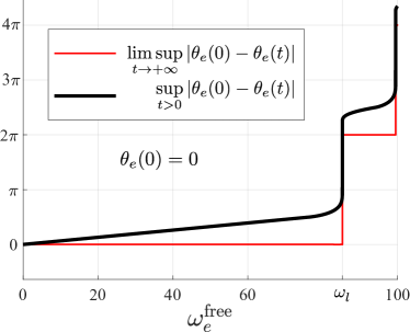
Figure 3: Comparison of cycle slipping definitions (see Remark 3.2) for model (2) with parameters $\tau_{1}=0.0633$, $\tau_{2}=0.0225$, $K_{\rm vco}=250$.

From a mathematical point of view, system (2) can initially be in an unstable equilibrium (at one of the saddles) or can acquire it by a separatrix after a change of $\omega_{e}^{\rm free}$ (see Kuznetsov et al. [2019a, 2020a]). Corresponding behavior is not observed in practice: system state is disturbed by noise and can’t remain in unstable equilibrium. In this paper, two cycle-slipping-related characteristics of the system are considered: the lock-in range $|\omega_{e}^{\rm free}|\in[0,\omega_{l})$ where the equilibria are considered to be stable and the conservative lock-in range $|\omega_{e}^{\rm free}|\in[0,\omega_{l}^{c})\subset[0,\omega_{l})$ which takes into account the unstable behavior described above.

For the considered model boundary values $\omega_{l}$ and $\omega_{l}^{c}$ are determined by cycle slipping bifurcation. It happens when the system being in an equilibrium state is exposed to an abrupt change of $\omega_{e}^{\rm free}$, and the corresponding trajectory of the system after the switch tends to the nearest unstable equilibrium by the corresponding saddle separatrix. In other words, $\sup\limits_{t>0}|\theta_{e}(0)-\theta_{e}(t)|=\limsup\limits_{t\to+\infty}|\theta_{e}(0)-\theta_{e}(t)|=\pi$ for $\theta_{e}(0)=2\pi$ (see Fig. 4, lower left picture) and $\sup\limits_{t>0}|\theta_{e}(0)-\theta_{e}(t)|=\limsup\limits_{t\to+\infty}|\theta_{e}(0)-\theta_{e}(t)|=2\pi$ for $\theta_{e}(0)=3\pi$ (see Fig. 4, upper right picture). For a larger $\omega_{e}^{\rm free}$ supremum $\sup\limits_{t>0}|\theta_{e}(0)-\theta_{e}(t)|>2\pi$ and cycle slipping occurs. Since the lock-in range is defined as a half-open interval, boundary values $\omega_{e}^{\rm free}=\omega_{l}$ and $\omega_{e}^{\rm free}=\omega_{l}^{c}$ are not included in it.

      

      

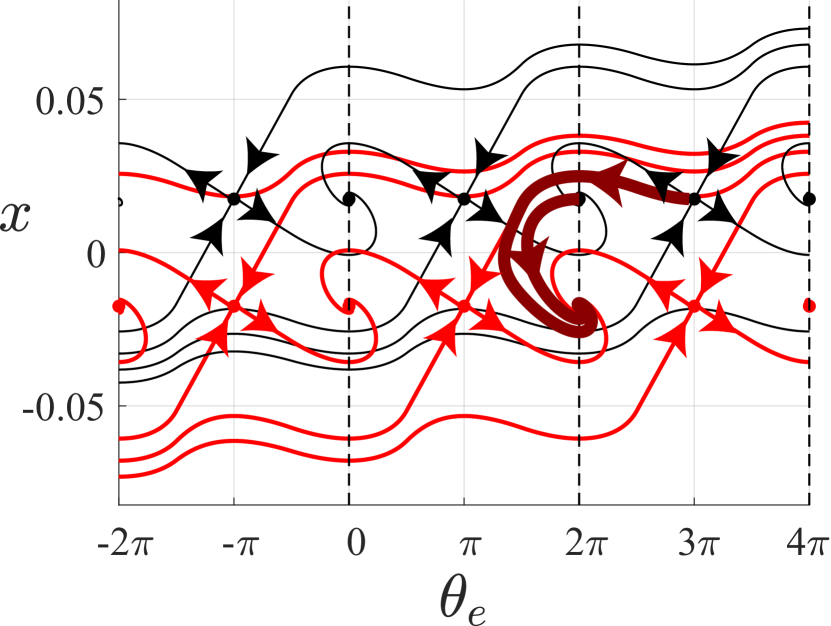
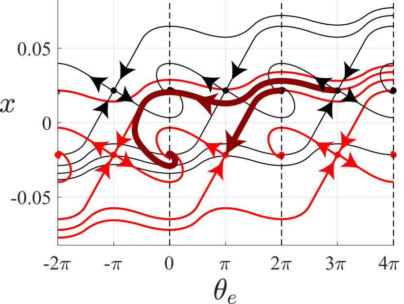
Figure 4: Phase portraits for model (2) with the following parameters: $F(s)=\frac{1+s\tau_{2}}{s\tau_{1}}$, $\tau_{1}=0.0633$, $\tau_{2}=0.0225$, $K_{\rm vco}=250$. Black dots are equilibria of the model with positive $\omega_{e}^{\rm free}=|\omega|$. Red color is for the model with negative $\omega_{e}^{\rm free}=-|\omega|$. Separatrices pass in and out of the saddles equilibria. Upper left subfigure: $\omega=69<\omega_{l}^{c}$, upper right subfigure: $\omega=\omega_{l}^{c}\approx 70.79$ (evaluated by Theorem 2), lower left subfigure: $\omega=\omega_{l}\approx 85.27$ (evaluated by Theorem 1), lower right subfigure: $\omega=86>\omega_{l}$.

In practice, the lock-in range can be estimated in the following way. Without loss of generality we can fix $\omega_{\rm vco}^{\rm free}$ and vary $\omega_{\rm ref}$ only. Let initially $\omega_{e}^{\rm free}=\omega_{\rm ref}-\omega_{\rm vco}^{\rm free}=0$ and the system is in a stable equilibrium. Then we abruptly increase the reference frequency by sufficiently small frequency step $\Delta\omega>0$ (i.e., the reference frequency becomes $\omega_{\rm ref}=\omega_{\rm vco}^{\rm free}+\Delta\omega$) and observe whether corresponding transient process converges to a locked state without cycle slipping (see Fig. LABEL:fig:lock-in-procedure). After that we abruptly decrease the reference frequency by $2\Delta\omega$ (i.e., the reference frequency becomes $\omega_{\rm ref}=\omega_{\rm vco}^{\rm free}-\Delta\omega$). If the transient process converges to the locked state without cycle slipping, then $[0,\Delta\omega)\subset[0,\omega_{l})$. Frequency step $\Delta\omega>0$ should be increased until cycle slipping occurs.

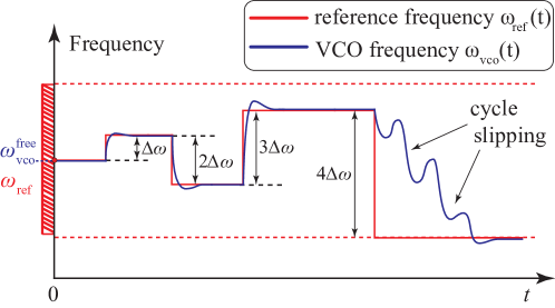
Figure 5: The lock-in range calculation.

Using changes of variables we represent system (2) as the first-order differential equation Belyustina [1959]; Huque & Stensby [2011] and following Aleksandrov et al. [2016]; Kuznetsov et al. [2019a] we formulate and prove theorems providing exact values for the lock-in range and for the conservative lock-in range.

Theorem 3.3.

The lock-in frequency of model (2) with the piecewise-linear PD characteristic (1) is

$$\omega_{l}=\begin{cases}&\frac{a\sqrt{\pi}}{2\tau_{2}}\Big{(}\frac{c+b}{c-b}\Big{)}^{\frac{a}{2b}},\quad a^{2}k>4,\\ &\frac{a\sqrt{\pi}}{2\tau_{2}}\exp(\frac{a}{2\sqrt{\pi}}),\quad a^{2}k=4,\\ &\frac{a\sqrt{\pi}}{2\tau_{2}}\exp\Big{(}{\frac{a}{b}\arctan\frac{b}{c}}\Big{)},\quad a^{2}k<4\end{cases}$$ (4)

where

$$a=\sqrt{\frac{K_{\rm{vco}}}{\tau_{1}}}\tau_{2},\quad b=\sqrt{|a^{2}-\frac{4}{k}|},\quad c=\sqrt{a^{2}+4(\pi-\frac{1}{k})}.$$ (5)

Theorem 3.4.

The conservative lock-in frequency of model (2) with piecewise-linear PD characteristic (1) is

$$\omega_{l}^{c}=\ \frac{1}{2}\sqrt{\frac{K_{\rm vco}(d+\frac{c-a}{2})^{\frac{c-a}{c}}(d-\frac{c+a}{2})^{\frac{c+a}{c}}}{\tau_{1}}},$$ (6)

where $a,\ b$ and $c$ are evaluated by (5), and $d$ is the unique solution of one of the equations:

$$\begin{cases}&(d-\frac{a-b}{2})^{\frac{b-a}{b}}(d-\frac{a+b}{2})^{\frac{b+a}{b}}=\pi(\frac{c+b}{c-b})^{\frac{a}{b}},\ d>\frac{a+b}{2},\quad a^{2}k>4,\\ &d=\frac{a}{2}\Big{(}1+\dfrac{1}{W(\frac{a}{2\sqrt{\pi}}\exp({-\frac{a}{2\sqrt{\pi}}}))}\Big{)},\quad a^{2}k=4,\\ &\Big{(}d^{2}-ad+\frac{1}{k}\Big{)}\exp\Big{(}\frac{2a}{b}\arctan\frac{b}{a-2d}\Big{)}=\pi\exp\Big{(}\frac{2a}{b}\arctan\frac{b}{c}\Big{)},\ d>\frac{a}{2},\quad a^{2}k<4.\end{cases}$$ (7)

Here $W(x)$ is the Lambert $W$ function.

Proof 3.5 (Proof of Theorem 3.3 and Theorem 3.4).

The proof given in Appendix A is based on the fact that system (2) is piecewise-linear and can be integrated analytically on the linear segments.

Notice that $\omega_{l}$ and $\omega_{l}^{c}$ are continuous functions of variable $k$ (as $a$ is fixed): the cases $a^{2}k>4$ and $a^{2}k<4$ in formulae (4), (6) approach the case $a^{2}k=4$ as $k\to\frac{4}{a^{2}}$ (as $b\to 0$).

4 Conclusions

In this work, the exact formulae for the lock-in range and the conservative lock-in range for the second-order type 2 PLL with a piecewise-linear phase detector characteristic were derived. In engineering literature, the following approximate estimate for the lock-in range can be found:

$$\omega_{l}\approx\frac{K_{\rm vco}\tau_{2}}{\tau_{1}}$$ (8)

(see [Best, 2007, p.69] where $\omega_{l}\approx\pi\zeta\omega_{n}$, $\omega_{n}=\sqrt{K_{d}K_{\rm vco}/\tau_{1}}$, $\zeta=\omega_{n}\tau_{2}/2$, $K_{d}=\frac{2}{\pi}$, and [Gardner, 2005, p.187] where $K_{d}=1,K_{o}=K_{\rm vco}$). However, estimate (8) intersects the exact lock-in frequency value (4) for some values of parameters. Taking into account that for type 2 PLLs a pull-out frequency $\omega_{\rm po}$ is twice the value of the lock-in frequency, one more approximate estimate for the lock-in range is exploited:

$$\omega_{l}\approx 0.7995\sqrt{\frac{2K_{\rm vco}}{\pi\tau_{1}}}+1.23\frac{\tau_{2}K_{\rm vco}}{\pi\tau_{1}}$$

(see [Best, 2007, p.84] where $2\omega_{l}=\omega_{\rm po}\approx 2.46\omega_{n}(\zeta+0.65)$, $\omega_{n}=\sqrt{K_{d}K_{\rm vco}/\tau_{1}},\ \zeta=\omega_{n}\tau_{2}/2,\ K_{d}=\frac{2}{\pi}$).

A.S. Huque and J. Stensby analysed system (2) with a triangular PD characteristic [the piecewise-linear PD characteristic (1) with $k=\frac{2}{\pi}$] in Huque & Stensby [2011]; Huque [2011]. However, in those works the global stability of system (2) was not analysed. In these works, the following formula for a pull-out frequency was derived:

$$\omega_{\rm po}=\frac{a^{2}}{\tau_{2}}\exp\Big{(}\frac{1}{2}\ln|m_{-}^{2}-m_{-}+a^{\prime}|-\frac{1}{\sqrt{4a^{\prime}-1}}\arctan\left(\frac{1-2m_{-}}{\sqrt{4a^{\prime}-1}}\right)+\frac{\pi}{2\sqrt{4a^{\prime}-1}}\Big{)}$$ (9)

where $a^{\prime}=\frac{\pi}{2a^{2}},\ m_{-}=\frac{1}{2}(1-\sqrt{4a^{\prime}+1})$. For $a^{2}<2\pi$ the lock-in frequency $\omega_{l}=\frac{1}{2}\omega_{\rm po}$ with $\omega_{\rm po}$ from (9) coincides with the corresponding case in (4), however for $a^{2}\geq 2\pi$ formula (9) is formally not applicable and equations (4) should be used.

It’s important to note that obtained lock-in range formula (4) is also a lower analytical estimate for the lock-in range of the second-order type 2 PLL with a sinusoidal PD characteristic. For these systems several engineering estimates are known (see, e.g., [Gardner, 2005, p.117] and Huque & Stensby [2013] for the pull-out range estimates, and [Gardner, 2005, p.187], [Kolumbán, 2005, p.3748], [Best, 2007, p.67], Best et al. [2016], [Best, 2018, p.18] for the lock-in range estimates).

The further development of such systems analysis is connected with consideration of higher-order loop filters and discontinuous phase detector characteristics for revealing hidden oscillations and providing the global stability Zhu et al. [2020]; Kuznetsov et al. [2021c].

Acknowledgments The work is funded by Team Finland Knowledge programme (163/83/2021) and by the Ministry of Science and Higher Education of the Russian Federation as part of World-class Research Center program: Advanced Digital Technologies (contract No. 075-15-2020-934 dated 17.11.2020). Z. Wei acknowledges support from the National Natural Science Foundation of China (Nos. 12172340 and 11772306).

Proof of Theorem 3.3 and Theorem 3.4

Proof .1 (Proof of Theorem 3.3 and Theorem 3.4).

Let’s find the lock-in range of model (2) with piecewise-linear PD characteristic (1). As it was noted in section 3, the lock-in frequency can be determined by such an abrupt change of $\omega_{e}^{\rm free}$ that the corresponding trajectory tends to the nearest unstable equilibrium (by the corresponding separatrix). Suppose that initially the frequency error was equal to $\omega_{e}^{\rm free}=-\omega<0$, but then changed to $\omega_{e}^{\rm free}=\omega>0$. Hence, initially the system is in equilibrium $x^{\rm eq}=-\frac{\tau_{1}\omega}{K_{\rm vco}},\quad\theta_{e}^{\rm eq}=0$, but after the switch the corresponding trajectory tends to $x^{\rm eq}=\frac{\tau_{1}\omega}{K_{\rm vco}},\quad\theta_{e}^{\rm eq}=0$ without cycle slipping if $\omega<\omega_{l}$.

Such $\omega_{l}$ is determined by such frequency error $\omega_{e}^{\rm free}$ that a trajectory being in stable equilibrium (before the switch) $x^{\rm eq}=-\frac{\tau_{1}\omega_{l}}{K_{\rm vco}},\quad\theta_{e}^{\rm eq}=0$ tends to saddle equilibrium (after the switch) $x^{\rm eq}=\frac{\tau_{1}\omega_{l}}{K_{\rm vco}},\quad\theta_{e}^{\rm eq}=\pi$ by the corresponding separatrix. Thus, the lock-in frequency $\omega_{l}$ corresponds to the case

$$-\frac{\tau_{1}\omega_{l}}{K_{\rm vco}}=Q(0,\omega_{l})$$ (10)

where $\frac{\tau_{1}\omega_{e}^{\rm free}}{K_{\rm vco}}$ is $x$-coordinate of equilibrium of model (2) and $x=Q(\theta_{e},\omega_{e}^{\rm free})$ is the lower separatrix of saddle equilibrium $(\frac{\tau_{1}\omega_{e}^{\rm free}}{K_{\rm vco}},\pi)$ (see Fig. 4).

After the change of variables $\tau=\sqrt{\frac{K_{\rm vco}}{\tau_{1}}}t$, $y=\sqrt{\frac{\tau_{1}}{K_{\rm vco}}}\omega_{e}^{\rm free}-\sqrt{\frac{K_{\rm vco}}{\tau_{1}}}(x+\tau_{2}v_{e}(\theta_{e}))$, for $\theta_{e}(t)\in(-\frac{1}{k}+2\pi n,\ \frac{1}{k}+2\pi n)$ and $\theta_{e}(t)\in(\frac{1}{k}+2\pi n,\ -\frac{1}{k}+2\pi(n+1))$ system (2) is represented as follows:

$$\dot{y}=-av_{e}^{\prime}(\theta_{e})y-v_{e}(\theta_{e}),$$ (11)

$$\dot{\theta}_{e}=y,$$

where $a=\tau_{2}\sqrt{\frac{K_{\rm{vco}}}{\tau_{1}}}$.

Upper separatrix $y=S(\theta_{e})$ of the phase plane of (11) corresponds to separatrix $x=Q(\theta_{e},\omega_{e}^{\rm free})$ from (2) (see Fig. 6) and has the form

$$S(\theta_{e})=\sqrt{\frac{\tau_{1}}{K_{\rm vco}}}\omega_{e}^{\rm free}-\sqrt{\frac{K_{\rm vco}}{\tau_{1}}}(Q(\theta_{e},\omega_{e}^{\rm free})+\tau_{2}v_{e}(\theta_{e})).$$

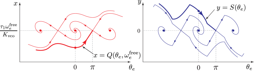
Figure 6: Phase plane portraits of (2) and (11).

Thus, relation (10) takes the form

$$-\frac{\tau_{1}\omega_{l}}{K_{\rm vco}}=\frac{\tau_{1}\omega_{l}}{K_{\rm vco}}-\sqrt{\frac{\tau_{1}}{K_{\rm vco}}}S(0).$$

Hence, $\omega_{l}=\frac{a}{2\tau_{2}}S(0)$. Analogously to the phase plane analysis for $\omega_{l}$, we get the following formula for the conservative lock-in frequency: $\omega_{l}^{c}=\frac{a}{2\tau_{2}}S(-\pi)$. Denote

$$y_{l}=S(0),\qquad y_{l}^{c}=S(-\pi)$$

and get the formulae for $\omega_{l}$ and $\omega_{l}^{c}$:

$$\omega_{l}=\frac{a}{2\tau_{2}}y_{l},$$ (12)

$$\omega_{l}^{c}=\frac{a}{2\tau_{2}}y_{l}^{c}.$$ (13)

The computation of $y_{l}$ and $y_{l}^{c}$ from formulae (12), (13) consists of the following stages. Let’s divide the phase plane to the following domains:

• I: $\{(y,\ \theta_{e})\mid\frac{1}{k}\leq\theta_{e}\leq\pi$; $\theta_{e},y\in\mathbb{R}\}$,

• II: $\{(y,\ \theta_{e})\mid-\frac{1}{k}\leq\theta_{e}\leq\frac{1}{k}$; $\theta_{e},y\in\mathbb{R}\}$,

• III: $\{(y,\ \theta_{e})\mid-\pi\leq\theta_{e}\leq-\frac{1}{k}$; $\theta_{e},y\in\mathbb{R}\}$.

In the open domains, system (11) is a linear one and can be integrated analytically. Firstly, we compute $S(\frac{1}{k})$, which is possible due to the continuity of (2). Using the obtained value as the initial data of the Cauchy problem and finding its solution in the domain II, we can compute $y_{l}=S(0)$ and $S(-\frac{1}{k})$. Here exist three cases depending on the stable equilibrium type: an asymptotically stable focus, an asymptotically stable node, and an asymptotically stable degenerated node. For every case described above we perform separate computations. Using the obtained value as the initial data of the Cauchy problem and finding its solution in the domain III, we can compute $y_{l}^{c}=S(-\pi)$ (see Fig. 7).

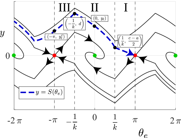
Figure 7: The separatrix integration. Firstly, we compute $S(\frac{1}{k})$ and use it as the initial data of the Cauchy problem. Secondly, finding its solution in the domain II, we compute $y_{l}=S(0)$, which is used for the lock-in frequency $\omega_{l}$ computation (see (12)), and $S(-\frac{1}{k})$. Finally, we use $S(-\frac{1}{k})$ as the initial data of the Cauchy problem and find its solution in the domain III, determining $y_{l}^{c}=S(-\pi)$, which is used for the conservative lock-in frequency $\omega_{l}^{c}$ computation (see (13)). Parameters: $\tau_{1}=0.0633$, $\tau_{2}=0.0225$, $K_{\rm vco}=250$, $k=\frac{2}{\pi}$.

Domain I.

The saddle separatrix is locally described by the saddle’s eigenvectors

$$V^{s}_{+}=\begin{pmatrix}1\\ \frac{c-a}{2}\end{pmatrix},\quad V^{s}_{-}=\begin{pmatrix}1\\ \frac{-c-a}{2}.\end{pmatrix}$$

Eigenvector $V^{s}_{-}$ points to a saddle and $V^{s}_{+}$ has the opposite direction. Since in the considered domain the system is a linear one, then the separatrix coincides with the line corresponding to $V_{-}^{s}$:

$$S(\theta_{e})=\frac{c-a}{2\left(\pi-\frac{1}{k}\right)}(\pi-\theta_{e}),\quad\frac{1}{k}<\theta_{e}<\pi.$$

Let’s obtain the limit value in $\theta_{e}=\frac{1}{k}$:

$$S(\frac{1}{k})=\frac{c-a}{2}>0.$$

Domain II. If $-\frac{1}{k}<\theta_{e}(t)<\frac{1}{k}$ then system (11) is

$$\dot{y}=-aky-k\theta_{e},$$ (14)

$$\dot{\theta}_{e}=y.$$

In the domains $\{y>0\}$ and $\{y<0\}$, variable $\theta_{e}(t)$ changes monotonically and the behaviour of system (14) can be described by the first-order differential equation:

$$\frac{dy}{d\theta_{e}}=-ak-\frac{k\theta_{e}}{y}.$$ (15)

The obtained equation is Chini’s equation Chini [1924]; Cheb-Terrab & Kolokolnikov [2003], which is a generalization of Abel and Riccati equations. The change of variables $z=\frac{y}{\theta_{e}}$ maps equation (15) into a separable one:

$$\frac{zdz}{z^{2}+akz+k}=-\frac{d\theta_{e}}{\theta_{e}}.$$ (16)

If $z^{2}+akz+k\neq 0$ then solutions of system (15) and system (16) coincide in domains $0<\theta_{e}<\frac{1}{k}$ and $-\frac{1}{k}<\theta_{e}<0$. Depending on the type of an asymptotically stable equilibrium, the following cases appear (see section 2.1):

• $a^{2}k>4$ (the equation $z^{2}+akz+k=0$ describes the eigenvectors of the stable node),

• $a^{2}k=4$ (the equation $z^{2}+akz+k=0$ describes the eigenvector of the stable degenerate node),

• $a^{2}k<4$ (here the case $z^{2}+akz+k=0$ is not possible).

Case $a^{2}k>4$. Let’s take into account the location of separatrix $y=S(\theta_{e})$, satisfying (15), during its integration on intervals. The eigenvectors of the stable node

$$V^{n}_{+}=\begin{pmatrix}1\\ -\frac{a-b}{2}\end{pmatrix},\quad V^{n}_{-}=\begin{pmatrix}1\\ -\frac{a+b}{2}\end{pmatrix}$$

are described by lines $y=-\frac{a+b}{2}k\theta_{e}$ and $y=-\frac{a-b}{2}k\theta_{e}$, respectively, and intersect the boundary $\theta_{e}=\frac{1}{k}$ of domains I and II in points $-\frac{a-b}{2}<0$ and $-\frac{a+b}{2}<0$. Hence, the separatrix, intersecting the boundary $\theta_{e}=\frac{1}{k}$ of domains I and II in point $\frac{c-a}{2}>0$, remains over the eigenvectors within the domain II and satisfies the following inequality: $(S(\theta_{e})+\frac{a+b}{2}k\theta_{e})(S(\theta_{e})+\frac{a-b}{2}k\theta_{e})>0$ as $\theta_{e}\in[-\frac{1}{k},\frac{1}{k}]$.

Assuming $(z+\frac{a+b}{2}k)(z+\frac{a-b}{2}k)>0$, the general solution of equation (16) is as follows :

$$N_{1}(z)=-\ln|\theta_{e}|+C$$

where

$$N_{1}(z)=\frac{1}{2}\ln\Big{(}\big{(}z+\frac{a-b}{2}k\big{)}^{\frac{b-a}{b}}\big{(}z+\frac{a+b}{2}k\big{)}^{\frac{b+a}{b}}\Big{)},\quad C={\rm const}.$$

Since for separatrix $y=S(\theta_{e})$ inequality $(y+\frac{a+b}{2}k\theta_{e})(y+\frac{a-b}{2}k\theta_{e})>0$ is valid, we get that the separatrix on interval $0<\theta_{e}(t)\leq\frac{1}{k}$ satisfies $N(y,\theta_{e})=C_{(0,\frac{1}{k})}$ where

$$N(y,\theta_{e})=\frac{1}{2}\ln\Big{(}\big{(}y+\frac{a-b}{2}k\theta_{e}\big{)}^{\frac{b-a}{b}}\big{(}y+\frac{a+b}{2}k\theta_{e}\big{)}^{\frac{b+a}{b}}\Big{)},$$

$$C_{(0,\frac{1}{k})}=\lim\limits_{\theta_{e}\to\frac{1}{k}-0}N(\frac{c-a}{2},\theta_{e})=\frac{1}{2}\ln\Big{(}(\frac{c-b}{2})^{\frac{b-a}{b}}(\frac{c+b}{2})^{\frac{b+a}{b}}\Big{)}=\frac{1}{2}\ln\Big{(}\pi(\frac{c+b}{c-b})^{\frac{a}{b}}\Big{)}.$$

Thus, if $a^{2}k>4$, then separatrix $y=S(\theta_{e})$ in domain $0<\theta_{e}(t)\leq\frac{1}{k}$ is described by equation

$$\big{(}y+\frac{a-b}{2}k\theta_{e}\big{)}^{\frac{b-a}{b}}\big{(}y+\frac{a+b}{2}k\theta_{e}\big{)}^{\frac{b+a}{b}}=\pi(\frac{c+b}{c-b})^{\frac{a}{b}}.$$ (17)

Substituting $\theta_{e}\to+0$ into (17), we get

$$y_{l}=\sqrt{\pi}(\frac{c+b}{c-b})^{\frac{a}{2b}}.$$ (18)

Then, substituting (18) into (12), we get the first case of formula (4).

To determine the conservative lock-in frequency, we firstly need to get $d=S(-\frac{1}{k})$, then to obtain the equation for the separatrix in domain III, and, finally, to determine $y_{l}^{c}=S(-\pi)$. Since the separatrix on interval $-\frac{1}{k}<\theta_{e}(t)<0$ satisfies $N(y,\theta_{e})=C_{(-\frac{1}{k},0)}$ and $\lim\limits_{\theta_{e}\to+0}N(y,\theta_{e})=\lim\limits_{\theta_{e}\to-0}N(y,\theta_{e})=\ln y$ as $y>0$, then $C_{(-\frac{1}{k},0)}=C_{(0,\frac{1}{k})}=\frac{1}{2}\ln\Big{(}\pi(\frac{c+b}{c-b})^{\frac{a}{b}}\Big{)}$.

Thus, if $a^{2}k>4$, then separatrix $y=S(\theta_{e})$ in domain II is described by equation (17). Substituting $\theta_{e}=-\frac{1}{k}$ into (17), we get

$$(d-\frac{a-b}{2})^{\frac{b-a}{b}}(d-\frac{a+b}{2})^{\frac{b+a}{b}}=\pi(\frac{c+b}{c-b})^{\frac{a}{b}}.$$ (19)

Since the separatrix is over the eigenvectors ($y>-\frac{a\pm b}{2}k\theta_{e}$), then

$$d>\frac{a+b}{2}.$$

Notice that if $d=\frac{a+b}{2}$, then the left-hand side of equation (19) equals to zero, but the right-hand side is positive. Then the left-hand side increases monotonically as value $d$ increases and tends to infinity as $d\to+\infty$. Thus, equation (19) has unique solution $d$ greater than $\frac{a+b}{2}$.

Case $a^{2}k=4$.

In domain II, separatrix $y=S(\theta_{e})$ is over eigenvector

$$V^{dn}=\begin{pmatrix}1\\ -\frac{a}{2}\end{pmatrix},$$

which is described by line $y=-\frac{2}{a}\theta_{e}$ and intersects the boundary $\theta_{e}=\frac{1}{k}$ of domains I and II in point $-\frac{a}{2}<0$. Hence, the separatrix, intersecting the boundary $\theta_{e}=\frac{1}{k}$ of domains I and II in point $\frac{c-a}{2}>0$, remains over the eigenvector within the domain II and satisfies the following inequality: $S(\theta_{e})>-\frac{2}{a}\theta_{e}$.

The general solution of (16) is as follows:

$$N_{1}(z)=-\ln|\theta_{e}|+C$$

where

$$N_{1}(z)=\frac{2}{2+az}+\ln|2+az|,\quad C={\rm const}.$$

Since for separatrix $y=S(\theta_{e})$ inequality $S(\theta_{e})>-\frac{2}{a}\theta_{e}$. is valid, we get that the separatrix on interval $0<\theta_{e}(t)\leq\frac{1}{k}$ satisfies $N(y,\theta_{e})=C_{(0,\frac{1}{k})}$ where

$$N(y,\theta_{e})=\frac{2\theta_{e}}{2\theta_{e}+ay}+\ln(2\theta_{e}+ay),$$

$$C_{(0,\frac{1}{k})}=\lim\limits_{\theta_{e}\to\frac{1}{k}-0}N(\frac{c-a}{2},\theta_{e})=\frac{2}{k}\frac{1}{\frac{2}{k}+a\sqrt{\pi}-\frac{a^{2}}{2}}+\ln(\frac{2}{k}+a\sqrt{\pi}-\frac{a^{2}}{2})=\frac{a}{2\sqrt{\pi}}+\ln(a\sqrt{\pi}).$$

Thus, if $a^{2}k=4$, then separatrix $y=S(\theta_{e})$ in domain $0<\theta_{e}(t)\leq\frac{1}{k}$ is described by equation

$$\frac{2\theta_{e}}{2\theta_{e}+ay}+\ln(2\theta_{e}+ay)=\frac{a}{2\sqrt{\pi}}+\ln(a\sqrt{\pi}).$$ (20)

Substituting $\theta_{e}\to+0$ into (20), we get

$$y_{l}=\sqrt{\pi}\exp(\frac{a}{2\sqrt{\pi}}).$$ (21)

Then, substituting (21) into (12), we get the second case of formula (4).

To determine the conservative lock-in frequency, we firstly need to determine $d=S(-\frac{1}{k})$. Since the separatrix on interval $-\frac{1}{k}<\theta_{e}(t)<0$ satisfies $N(y,\theta_{e})=C_{(-\frac{1}{k},0)}$ and $\lim\limits_{\theta_{e}\to+0}N(y,\theta_{e})=\lim\limits_{\theta_{e}\to-0}N(y,\theta_{e})=\ln(ay)$ as $y>0$, then $C_{(-\frac{1}{k},0)}=C_{(0,\frac{1}{k})}=\frac{a}{2\sqrt{\pi}}+\ln(a\sqrt{\pi})$.

Thus, if $a^{2}k=4$, then separatrix $y=S(\theta_{e})$ in domain II is described by equation (20). Substituting $\theta_{e}=-\frac{1}{k}$ into (20), we get

$$(d-\frac{a}{2})\exp\Big{(}\frac{\frac{a}{2}}{\frac{a}{2}-d}\Big{)}=\sqrt{\pi}e^{\frac{a}{2\sqrt{\pi}}}.$$

Notice that in the considered case it is possible to obtain an explicit formula for $d$:

$$d=\frac{a}{2}\Big{(}1+\frac{1}{W(\frac{a}{2\sqrt{\pi}}\exp(-\frac{a}{2\sqrt{\pi}})}\Big{)}$$ (22)

where $W(x)$ is the Lambert W function.

Case $a^{2}k<4$.

The general solution of (15) is as follows:

$$N_{1}(z)=-\ln|\theta_{e}|+C$$

where

$$N_{1}(z)=\frac{1}{2}\ln(z^{2}+akz+k)-\frac{a}{b}\arctan(\frac{a+\frac{2}{k}z}{b}),\quad C={\rm const}.$$

Then separatrix $y=S(\theta_{e})$ in domain $0<\theta_{e}\leq\frac{1}{k}$ satisfies $N(y,\theta_{e})=C_{(0,\ \frac{1}{k})}$ where

$$N(y,\theta_{e})=\frac{1}{2}\ln(y^{2}+aky\theta_{e}+k\theta^{2}_{e})-\frac{a}{b}\arctan\Big{(}\frac{a\theta_{e}+\frac{2}{k}y}{b\theta_{e}}\Big{)},$$

$$C_{(0,\ \frac{1}{k})}=\lim\limits_{\theta_{e}\to\frac{1}{k}-0}N(\frac{c-a}{2},\theta_{e})=\frac{1}{2}\ln\pi-\frac{a}{b}\arctan\frac{c}{b}.$$

Thus, if $a^{2}k<4$, then separatrix $y=S(\theta_{e})$ in domain $0<\theta_{e}\leq\frac{1}{k}$ is described by equation

$$\frac{1}{2}\ln(y^{2}+aky\theta_{e}+k\theta^{2}_{e})-\frac{a}{b}\arctan\Big{(}\frac{a\theta_{e}+\frac{2}{k}y}{b\theta_{e}}\Big{)}=\frac{1}{2}\ln\pi-\frac{a}{b}\arctan\frac{c}{b}.$$ (23)

Substituting $\theta_{e}\to+0$ into (23), we get

$$y_{l}=\sqrt{\pi}\exp\Big{(}{\frac{a}{b}\arctan\frac{b}{c}}\Big{)}.$$ (24)

Then, substituting (24) into (12), we get the third case of formula (4). Thus, Theorem 3.3 is proved.

To determine the conservative lock-in frequency, we firstly need to determine $d=S(-\frac{1}{k})$. Since the separatrix on interval $-\frac{1}{k}<\theta_{e}(t)<0$ satisfies $N(y,\theta_{e})=C_{(-\frac{1}{k},0)}$ and $\lim\limits_{\theta_{e}\to+0}N(y,\theta_{e})=\ln y-\frac{\pi a}{2b}$, $\lim\limits_{\theta_{e}\to-0}N(y,\theta_{e})=\ln y+\frac{\pi a}{2b}$, then $C_{(-\frac{1}{k},0)}-\frac{\pi a}{2b}=C_{(0,\frac{1}{k})}+\frac{\pi a}{2b}$.

Thus, if $a^{2}k<4$, then separatrix $y=S(\theta_{e})$ in domain II is described by

$$\frac{1}{2}\ln(y^{2}+aky\theta_{e}+k\theta^{2}_{e})-\frac{a}{b}\arctan\Big{(}\frac{a\theta_{e}+\frac{2}{k}y}{b\theta_{e}}\Big{)}=\frac{1}{2}\ln\pi-\frac{a}{b}\arctan\frac{c}{b},\quad\text{if}\;0<\theta_{e}(t)\leq\frac{1}{k}$$ (25)

$$y=y_{l},\quad\text{if}\;\theta_{e}(t)=0$$

$$\frac{1}{2}\ln(y^{2}+aky\theta_{e}+k\theta^{2}_{e})-\frac{a}{b}\arctan\Big{(}\frac{a\theta_{e}+\frac{2}{k}y}{b\theta_{e}}\Big{)}=\frac{1}{2}\ln\pi+\frac{a}{b}\Big{(}\pi-\arctan\frac{c}{b}\Big{)},\quad\text{if}\;-\frac{1}{k}\leq\theta_{e}(t)<0.$$

Substituting $\theta_{e}=-\frac{1}{k}$ into (25), we get

$$\Big{(}d^{2}-ad+\frac{1}{k}\Big{)}\exp\Big{(}\frac{2a}{b}\arctan\frac{2d-a}{b}-\frac{\pi a}{b}\Big{)}=\pi\exp\Big{(}\frac{2a}{b}\arctan\frac{b}{c}\Big{)}.$$ (26)

Notice that if $d=0$, then the left-hand side of equation (19) is less than the right-hand side:

$$\frac{1}{k}\exp\Big{(}\frac{2a}{b}\arctan\frac{-a}{b}-\frac{\pi a}{b}\Big{)}<\frac{1}{k}<\pi<\pi\exp\Big{(}\frac{2a}{b}\arctan\frac{b}{c}\Big{)}.$$

Then the left-hand side increases monotonically as value $d$ increases and tends to infinity as $d\to+\infty$. Thus, equation (26) has unique positive solution $d$.

Notice also that if $d=\frac{a}{2}$, then the left-hand side of equation (19) is less than the right-hand side too:

$$b^{2}\exp(-\frac{\pi a}{b})<a^{2}\exp(-\frac{\pi a}{b})<4\pi\exp(-\frac{\pi a}{b})<4\pi\frac{b^{2}}{\pi^{2}a^{2}}<\frac{4}{\pi}<\pi<\pi\exp\Big{(}\frac{2a}{b}\arctan\frac{b}{c}\Big{)}.$$

Thus, $d>\frac{a}{2}$ and equation (26) can be reduced to the following:

$$\Big{(}d^{2}-ad+\frac{1}{k}\Big{)}\exp\Big{(}\frac{2a}{b}\arctan\frac{b}{a-2d}\Big{)}=\pi\exp\Big{(}\frac{2a}{b}\arctan\frac{b}{c}\Big{)}.$$ (27)

Domain III

If $-\pi\leq\theta_{e}(t)<-\frac{1}{k}$ then system (11) is

$$\dot{y}=\frac{a}{\pi-\frac{1}{k}}y+\frac{1}{\pi-\frac{1}{k}}(\theta_{e}+\pi),$$ (28)

$$\dot{\theta_{e}}=y.$$

Analogously to the analysis in domain II, let’s study for $y>0$ the first-order differential equation

$$\frac{dy}{d\theta_{e}}=\frac{1}{\pi-\frac{1}{k}}(a+\frac{\theta_{e}+\pi}{y})$$ (29)

and make the change of variables $z=\frac{y}{\theta_{e}+\pi}$ mapping equation (29) into a separable one:

$$(\pi-\frac{1}{k})\frac{zdz}{\left(\pi-\frac{1}{k}\right)z^{2}-az-1}=-\frac{d\theta_{e}}{\theta_{e}+\pi}.$$ (30)

If $-\pi<\theta_{e}(t)<-\frac{1}{k}$ then the solutions of system (29) and system (30) coincide.

Separatrix $y=S(\theta_{e})$ is over the separatrices of saddle $(0,\ -\pi)$, which are described by the equations

$$y=\frac{\pm c-a}{2(\pi-\frac{1}{k})}(-\pi-\theta_{e}),\quad-\pi<\theta_{e}<-\frac{1}{k}.$$

Thus, the following inequality is valid for the separatrix: $(S(\theta_{e})+\frac{c-a}{2(\pi-\frac{1}{k})}(\pi+\theta_{e}))(S(\theta_{e})-\frac{c+a}{2(\pi-\frac{1}{k})}(\pi+\theta_{e}))>0$.

Assuming $(z+\frac{c-a}{2(\pi-\frac{1}{k})})(z-\frac{c+a}{2(\pi-\frac{1}{k})})>0$, the general solution of equation (30) is as follows:

$$M_{1}(z)=-\ln|\theta_{e}+\pi|+C$$

where

$$M_{1}(z)=\frac{1}{2}\ln\Big{(}\big{(}z+\frac{c-a}{2(\pi-\frac{1}{k})}\big{)}^{\frac{c-a}{c}}\big{(}z-\frac{c+a}{2(\pi-\frac{1}{k})}\big{)}^{\frac{c+a}{c}}\Big{)},$$

$$C={\rm const}.$$

Since for separatrix $y=S(\theta_{e})$ inequality $(y+\frac{c-a}{2(\pi-\frac{1}{k})}(\pi+\theta_{e}))(y-\frac{c+a}{2(\pi-\frac{1}{k})}(\pi+\theta_{e}))>0$ is valid, we get that the separatrix in domain III satisfies $M(y,\theta_{e})=C_{\left(-\pi,-\frac{1}{k}\right)}$ where

$$M(y,\theta_{e})=\frac{1}{2}\ln\Big{(}\Big{(}y+\frac{c-a}{2(\pi-\frac{1}{k})}(\pi+\theta_{e})\Big{)}^{\frac{c-a}{c}}\Big{(}y-\frac{c+a}{2(\pi-\frac{1}{k})}(\pi+\theta_{e})\Big{)}^{\frac{c+a}{c}}\Big{)},$$

$$C=C_{\left(-\pi,-\frac{1}{k}\right)}=\lim_{\theta_{e}\to-\frac{1}{k}-0}M(d,\theta_{e})=\frac{1}{2}\ln\Big{(}(d+\frac{c-a}{2})^{\frac{c-a}{c}}(d-\frac{c+a}{2})^{\frac{c+a}{c}}\Big{)}.$$

Thus, separatrix $y=S(\theta_{e})$ in domain III is described by equation

$$\Big{(}y+\frac{c-a}{2(\pi-\frac{1}{k})}(\pi+\theta_{e})\Big{)}^{\frac{c-a}{c}}\Big{(}y-\frac{c+a}{2(\pi-\frac{1}{k})}(\pi+\theta_{e})\Big{)}^{\frac{c+a}{c}}=(d+\frac{c-a}{2})^{\frac{c-a}{c}}(d-\frac{c+a}{2})^{\frac{c+a}{c}}.$$ (31)

To determine the conservative lock-in frequency, we firstly need to determine $y_{l}^{c}=S(-\pi)$. Substituting $\theta_{e}=-\pi$ into (31), we get

$$y_{l}^{c}=(d+\frac{c-a}{2})^{\frac{c-a}{2c}}(d-\frac{c+a}{2})^{\frac{c+a}{2c}}.$$ (32)

Substituting (32) into (13) and taking into account formulae (19), (22), (27), we get (6).

Theorem 3.3 and Theorem 3.4 are proved.

Octave code for Fig. 7 Code below can be runned on https://octave-online.net/ in order to obtain phase portrait on Fig. 7 and verify formulae (4) and (6). The code simulates trajectories of system (11) numerically and additionally plots two points: $(0,y_{l})$ and $(-\pi,y_{l}^{c})$ where $y_{l}$ and $y_{l}^{c}$ are used in lock-in range formulae (12) and (13). Since these points are lying on the separatrices, formulae (12) and (13) are validated numerically.

⬇

clear all;

close all;

clc;

% VCO input gain

K_vco = 250;

% Loop filter transfer function F(s) = (1+s tau_2)/(s tau_1), tau_1 > 0,

% tau_2 > 0

tau_2 = 0.0225;

tau_1 = 0.0633;

% The slope coefficient of piecewise-linear PD characteristic

% it becomes triangular with this coefficient

k=2/pi;

function y = draw_saddles_symmetric(ode, saddle, V, periods, options)

% draw_saddles_symmetric draws phase portrait of the system ode,

% starting from saddle with eigenvectors V for given number of periods

% options are used to tune ODE solver

% Integration time

TIME_POSITIVE = 0:0.005:20;

TIME_NEGATIVE = 0:-0.005:-20;

v1 = 0.01 .* flip(V(:,1)’);

␣␣␣␣v2␣=␣0.01␣.*␣flip(V(:,2)’);

␣␣␣␣%␣Calculate␣saddle␣separatrices␣and␣plot␣them

␣␣␣␣[T_1,␣X_1]␣=␣ode45(ode,␣TIME_NEGATIVE,␣saddle+v1,␣options);

␣␣␣␣[T_3,␣X_3]␣=␣ode45(ode,␣TIME_NEGATIVE,␣saddle-v1,␣options);

␣␣␣␣for␣j=1:length(periods)

␣␣␣␣␣␣␣␣plot(X_1(:,2)+periods(j),X_1(:,1));

␣␣␣␣␣␣␣␣plot(X_3(:,2)+periods(j),X_3(:,1));

␣␣␣␣end

␣␣␣␣[T_2,␣X_2]␣=␣ode45(ode,␣TIME_POSITIVE,␣saddle+v2,␣options);

␣␣␣␣[T_4,␣X_4]␣=␣ode45(ode,␣TIME_POSITIVE,␣saddle-v2,␣options);

␣␣␣␣for␣j=1:length(periods)

␣␣␣␣␣␣␣plot(X_2(:,2)+periods(j),␣X_2(:,1));

␣␣␣␣␣␣␣plot(X_4(:,2)+periods(j),␣X_4(:,1));

␣␣␣␣end

end

function␣y␣=␣sawtooth_diff(t)

%␣sawtooth_diff␣-␣the␣derivative␣of␣a␣triangular␣function

%␣(sawtooth␣(T,␣WIDTH)␣from␣signal␣package)

␣␣remain␣=␣abs(rem(t,␣2*pi));

␣␣if␣(pi/2␣<=␣remain␣&&␣remain␣<=␣3*pi/2)

␣␣␣␣␣␣y␣=␣-2/pi;

␣␣else

␣␣␣␣␣␣y␣=␣2/pi;

␣␣end

end

%␣PD␣characteristic

v_e␣=␣@(theta_e)␣(sawtooth(theta_e+pi/2,0.5));

%␣The␣derivative␣of␣PD␣characteristic

dv_e␣=␣@(theta_e)␣(sawtooth_diff(theta_e));

period␣=␣2*pi;

%␣Parameters␣a,␣b,␣c␣from␣Theorem␣1␣and␣2

a␣=␣sqrt(K_vco/tau_1)*tau_2;

b␣=␣sqrt(abs(a^2-4/k));

c␣=␣sqrt(a^2-4/k␣+␣4*pi);

%␣Computing␣the␣lock-in␣range␣and␣the␣concervative␣lock-in␣range␣by

%␣Theorem␣1␣and␣2

syms␣x;

if␣a^2*k>4

␣␣␣␣y_l␣=␣sqrt(pi)*␣((c+b)/(c-b))^(a/(2*b));

␣␣␣␣fcn␣=␣@(x)␣(x␣-␣(a-b)/2)^((b-a)/b)␣*␣(x␣-␣(a+b)/2)^((b+a)/b)␣-…

␣␣␣␣␣␣␣␣pi*((c+b)/(c-b))^(a/b);

␣␣␣␣init_param␣=␣[(a+b)/2,␣10000000];

␣␣␣␣%␣vpasolve␣numerically␣solves␣implicit␣equations␣with␣initial␣guess

␣␣␣␣%␣init_param␣(it␣was␣proven␣that␣the␣equation␣has␣a␣unique␣solution

␣␣␣␣%␣for␣x␣>␣(a+b)/2)

␣␣␣␣d␣=␣vpasolve(fcn(x),␣x,␣init_param);

else

␣␣␣␣if␣a^2*k␣==␣4

␣␣␣␣␣␣␣␣y_l␣=␣sqrt(pi)*exp(a/2/sqrt(pi));

␣␣␣␣␣␣␣␣d␣=␣a/2*(1␣+␣1/lambertw(a/2/sqrt(pi)*exp(-a/2/sqrt(pi))));

else

␣␣␣␣␣␣␣␣y_l␣=␣sqrt(pi)*exp(a*atan(b/c)/b);

␣␣␣␣␣␣␣␣fcn␣=␣@(x)␣((x)^2␣-␣a*x␣+␣1/k)␣*␣exp(␣2*a/b*atan((2*x-a)/b)␣-␣pi*a/b)␣-…

␣␣␣␣␣␣␣␣pi*exp(2*a/b*atan(b/c));

␣␣␣␣␣␣␣␣init_param␣=␣[a/2,␣10000000];

␣␣␣␣␣␣␣␣%␣vpasolve␣numerically␣solves␣implicit␣equations␣with␣initial␣guess

␣␣␣␣␣␣␣␣%␣init_param␣(it␣was␣proven␣that␣the␣equation␣has␣a␣unique␣solution

␣␣␣␣␣␣␣␣%␣for␣x␣>␣a/2)

␣␣␣␣␣␣␣␣d␣=␣vpasolve(fcn(x),␣x,␣init_param);

␣␣␣␣end

end

y_l_c␣=␣(d-0.5*(a-c))^((c-a)/c/2)␣*␣(d-0.5*(a+c))^((c+a)/c/2);

h␣=␣figure(1);

hold␣on;

grid␣on;

%␣Ploting␣two␣points␣which␣correspond␣the␣lock-in␣range␣and␣the␣conservative

%␣lock-in␣range

plot([0],␣[y_l],␣’k.’,␣’MarkerSize’,␣20);

plot([-pi],␣[eval(y_l_c)],␣’k.’,␣’MarkerSize’,␣20);

%␣System␣establishment␣for␣numerocal␣integration

%␣y␣=␣x(1),␣theta_e␣=␣x(2)

pll_s␣=␣@(t,x)([-␣a*dv_e(x(2))*x(1)␣-␣v_e(x(2));

␣␣␣␣␣␣␣␣␣␣␣␣␣␣␣␣␣x(1)]);

%␣One␣of␣the␣asymptotically␣stable␣equilibria

theta_eq␣=␣0;

x_eq␣=␣0;

%␣Draw␣phase␣portrait

saddles␣=␣[x_eq,␣-theta_eq+period/2-2*period;…

␣␣␣␣x_eq,␣-theta_eq+period/2-period;…

␣␣␣␣x_eq,␣-theta_eq+period/2;…

␣␣␣␣x_eq,␣-theta_eq+period/2+period;…

␣␣␣␣x_eq,␣-theta_eq+period/2+2*period];

focuses␣=␣[x_eq,␣theta_eq-period;…

␣␣␣␣x_eq,␣theta_eq-period;…

␣␣␣␣x_eq,␣theta_eq;…

␣␣␣␣x_eq,␣theta_eq+period;…

␣␣␣␣x_eq,␣theta_eq+2*period];

plot(-focuses(:,2),␣-focuses(:,1),␣’r.’,␣’MarkerSize’,␣20);

plot(focuses(:,2),␣focuses(:,1),␣’k.’,␣’MarkerSize’,␣20);

plot(-saddles(:,2),␣-saddles(:,1),␣’r.’,␣’MarkerSize’,␣20);

plot(saddles(:,2),␣saddles(:,1),␣’k.’,␣’MarkerSize’,␣20);

%␣Jacobian␣matrix␣of␣the␣system

A␣=␣[0␣1;

␣␣␣␣2/pi␣2*a/pi];

%␣Calculating␣saddle␣eigenvectors␣V

[V,␣D]␣=␣eig(A);

%␣Custom␣simulation␣options

options␣=␣odeset(’MaxStep’,␣0.001,␣’RelTol’,␣2e-7,␣’AbsTol’,␣2e-7);

draw_saddles_symmetric(pll_s,…

␣␣␣␣[x_eq,period/2-theta_eq],␣␣…

␣␣␣␣V,␣…

␣␣␣␣[-2*period,-period,0,period,2*period],…

␣␣␣␣options);

%␣Plot␣adjustments

axis([-2*pi␣2*pi␣-5␣5])

xticks([-4*pi␣-3*pi␣-2*pi␣-pi␣0␣pi␣2*pi,␣4*pi])

xticklabels({’-4\pi’,’-3\pi’,’-2\pi’,’-\pi’,’0’,’\pi’,’2\pi’,’4\pi’})

xlabel(’\theta_e’);

ylabel(’y’);

References

- Aleksandrov et al. [2016] Aleksandrov, K., Kuznetsov, N., Leonov, G., Neittaanmaki, N., Yuldashev, M. & Yuldashev, R. [2016] “Computation of the lock-in ranges of phase-locked loops with PI filter,” IFAC-PapersOnLine 49, 36–41, 10.1016/j.ifacol.2016.07.971.
- Alexandrov et al. [2015] Alexandrov, K., Kuznetsov, N., Leonov, G., Neittaanmaki, P. & Seledzhi, S. [2015] “Pull-in range of the PLL-based circuits with proportionally-integrating filter,” IFAC-PapersOnLine 48, 720–724, 10.1016/j.ifacol.2015.09.274.
- Andronov et al. [1937] Andronov, A., Vitt, E. & Khaikin, S. [1937] Theory of Oscillators (in Russian) (ONTI NKTP SSSR), [English transl.: 1966, Pergamon Press].
- Bakaev [1963] Bakaev, Y. [1963] “Stability and dynamical properties of astatic frequency synchronization system,” Radiotekhnika i Elektronika (in Russian) 8, 513–516.
- Belyustina [1959] Belyustina, L. [1959] “The study of a nonlinear pll system,” Izv. vuzov. Radiofizika (in Russian) 2, 277–291.
- Best [2007] Best, R. [2007] Phase locked loops: design, simulation, and applications (McGraw-Hill Professional).
- Best [2018] Best, R. [2018] Costas Loops: Theory, Design, and Simulation (Springer International Publishing).
- Best et al. [2016] Best, R., Kuznetsov, N., Leonov, G., Yuldashev, M. & Yuldashev, R. [2016] “Tutorial on dynamic analysis of the Costas loop,” IFAC Annual Reviews in Control 42, 27–49, 10.1016/j.arcontrol.2016.08.003.
- Cheb-Terrab & Kolokolnikov [2003] Cheb-Terrab, E. & Kolokolnikov, T. [2003] “First-order ordinary differential equations, symmetries and linear transformations,” European Journal of Applied Mathematics 14, 231–246.
- Chen et al. [2017] Chen, G., Kuznetsov, N., Leonov, G. & Mokaev, T. [2017] “Hidden attractors on one path: Glukhovsky-Dolzhansky, Lorenz, and Rabinovich systems,” International Journal of Bifurcation and Chaos in Applied Sciences and Engineering 27, art. num. 1750115.
- Chini [1924] Chini, M. [1924] “Sull’integrazione di alcune equazioni differenziali del primo ordine,” Rendiconti Instituto Lombardo (2) 57, 506–511.
- Du & Swamy [2010] Du, K. & Swamy, M. [2010] Wireless Communication Systems: from RF subsystems to 4G enabling technologies (Cambridge University Press).
- Egan [1981] Egan, W. [1981] Frequency synthesis by phase lock, 1st ed. (John Wiley & Sons, New York).
- Egan [2007] Egan, W. [2007] Phase-Lock Basics, 2nd ed. (John Wiley & Sons, New York).
- Gardner [1966] Gardner, F. [1966] Phaselock Techniques (John Wiley & Sons, New York).
- Gardner [2005] Gardner, F. [2005] Phaselock Techniques, 3rd ed. (John Wiley & Sons, New York).
- Gubar’ [1961] Gubar’, N. [1961] “Investigation of a piecewise linear dynamical system with three parameters,” Journal of Applied Mathematics and Mechanics 25, 1011–1023.
- Huque [2011] Huque, A. [2011] A new derivation of the pull-out frequency for second-order phase lock loops employing triangular and sinusoidal phase detectors (The University of Alabama in Huntsville), Ph. D. thesis.
- Huque & Stensby [2011] Huque, A. & Stensby, J. [2011] “An exact formula for the pull-out frequency of a 2nd-order type II phase lock loop,” IEEE Communications Letters 15, 1384–1387.
- Huque & Stensby [2013] Huque, A. & Stensby, J. [2013] “An analytical approximation for the pull-out frequency of a PLL employing a sinusoidal phase detector,” ETRI Journal 35, 218–225.
- Kaplan & Hegarty [2017] Kaplan, E. & Hegarty, C. [2017] Understanding GPS/GNSS: Principles and Applications, 3rd ed. (Artech House).
- Kapranov [1956] Kapranov, M. [1956] “The lock-in band of a phase locked loop,” Radiotekhnika (in Russian) 11, 37–52.
- Karimi-Ghartemani [2014] Karimi-Ghartemani, M. [2014] Enhanced phase-locked loop structures for power and energy applications (John Wiley & Sons).
- Kolumbán [2005] Kolumbán, G. [2005] The Encyclopedia of RF and Microwave Engineering, Phase-locked loops, Vol. 4 (John Wiley & Sons, New-York).
- Kuznetsov [2020] Kuznetsov, N. [2020] “Theory of hidden oscillations and stability of control systems,” Journal of Computer and Systems Sciences International , 647–66810.1134/S1064230720050093.
- Kuznetsov et al. [2019a] Kuznetsov, N., Blagov, M., Alexandrov, K., Yuldashev, M. & Yuldashev, R. [2019a] “Lock-in range of classical PLL with piecewise-linear phase detector characteristic,” Differencialnie Uravnenia i Protsesy Upravlenia (Differential Equations and Control Processes) , 74–89.
- Kuznetsov et al. [2022] Kuznetsov, N., Kolumbán, G., Belyaev, Y., Tulaev, A., Yuldashev, M. & Yuldashev, R. [2022] “Estimation of PLL impact on MEMS-gyroscopes parameters,” Gyroscopy and Navigation (in print).
- Kuznetsov et al. [2015] Kuznetsov, N., Leonov, G., Yuldashev, M. & Yuldashev, R. [2015] “Rigorous mathematical definitions of the hold-in and pull-in ranges for phase-locked loops,” IFAC-PapersOnLine 48, 710–713, 10.1016/j.ifacol.2015.09.272.
- Kuznetsov et al. [2017] Kuznetsov, N., Leonov, G., Yuldashev, M. & Yuldashev, R. [2017] “Hidden attractors in dynamical models of phase-locked loop circuits: limitations of simulation in MATLAB and SPICE,” Communications in Nonlinear Science and Numerical Simulation 51, 39–49, 10.1016/j.cnsns.2017.03.010.
- Kuznetsov et al. [2019b] Kuznetsov, N., Lobachev, M., Yuldashev, M. & Yuldashev, R. [2019b] “On the Gardner problem for phase-locked loops,” Doklady Mathematics 100, 568–570, 10.1134/S1064562419060218.
- Kuznetsov et al. [2021a] Kuznetsov, N., Lobachev, M., Yuldashev, M. & Yuldashev, R. [2021a] “The Egan problem on the pull-in range of type 2 PLLs,” Transactions on Circuits and Systems II: Express Briefs 68, 1467–1471, 10.1109/TCSII.2020.3038075.
- Kuznetsov et al. [2020a] Kuznetsov, N., Lobachev, M., Yuldashev, M., Yuldashev, R. & Kolumbán, G. [2020a] “Harmonic balance analysis of pull-in range and oscillatory behavior of third-order type 2 analog PLLs,” IFAC-PapersOnLine 53, 6378–6383.
- Kuznetsov et al. [2020b] Kuznetsov, N., Lobachev, M., Yuldashev, M., Yuldashev, R., Kudryashova, E., Kuznetsova, O., Rosenwasser, E. & Abramovich, S. [2020b] “The birth of the global stability theory and the theory of hidden oscillations,” 2020 European Control Conference Proceedings, pp. 769–774, 10.23919/ECC51009.2020.9143726.
- Kuznetsov et al. [2021b] Kuznetsov, N., Lobachev, M., Yuldashev, M., Yuldashev, R., Volskiy, S. & Sorokin, D. [2021b] “On the generalized Gardner problem for phase-locked loops in electrical grids,” Doklady Mathematics 103, 157–161.
- Kuznetsov et al. [2021c] Kuznetsov, N., Matveev, A., Yuldashev, M. & Yuldashev, R. [2021c] “Nonlinear analysis of charge-pump phase-locked loop: The hold-in and pull-in ranges,” IEEE Transactions on Circuits and Systems I: Regular Papers 68, 4049–4061, 10.1109/TCSI.2021.3101529.
- Kuznetsov et al. [2020c] Kuznetsov, N., Volskiy, S., Sorokin, D., Yuldashev, M. & Yuldashev, R. [2020c] “Power supply system for aircraft with electric traction,” 2020 21st International Scientific Conference on Electric Power Engineering (EPE), pp. 1–5, 10.1109/EPE51172.2020.9269181.
- Leonov & Kuznetsov [2013] Leonov, G. & Kuznetsov, N. [2013] “Hidden attractors in dynamical systems. From hidden oscillations in Hilbert-Kolmogorov, Aizerman, and Kalman problems to hidden chaotic attractors in Chua circuits,” International Journal of Bifurcation and Chaos in Applied Sciences and Engineering 23, 10.1142/S0218127413300024, art. no. 1330002.
- Leonov & Kuznetsov [2014] Leonov, G. & Kuznetsov, N. [2014] Nonlinear mathematical models of phase-locked loops. Stability and oscillations (Cambridge Scientific Publishers).
- Leonov et al. [2012] Leonov, G., Kuznetsov, N., Yuldashev, M. & Yuldashev, R. [2012] “Analytical method for computation of phase-detector characteristic,” IEEE Transactions on Circuits and Systems - II: Express Briefs 59, 633–647, 10.1109/TCSII.2012.2213362.
- Leonov et al. [2015a] Leonov, G., Kuznetsov, N., Yuldashev, M. & Yuldashev, R. [2015a] “Hold-in, pull-in, and lock-in ranges of PLL circuits: rigorous mathematical definitions and limitations of classical theory,” IEEE Transactions on Circuits and Systems–I: Regular Papers 62, 2454–2464, 10.1109/TCSI.2015.2476295.
- Leonov et al. [2015b] Leonov, G., Kuznetsov, N., Yuldashev, M. & Yuldashev, R. [2015b] “Nonlinear dynamical model of Costas loop and an approach to the analysis of its stability in the large,” Signal Processing 108, 124–135, 10.1016/j.sigpro.2014.08.033.
- Rosenkranz & Schaefer [2016] Rosenkranz, W. & Schaefer, S. [2016] “Receiver design for optical inter-satellite links based on digital signal processing,” 18th International Conference on Transparent Optical Networks (ICTON) (IEEE), pp. 1–4.
- Shakhtarin [1969] Shakhtarin, B. [1969] “Study of a piecewise-linear system of phase-locked frequency control,” Radiotechnica and electronika (in Russian) , 1415–1424.
- Stensby [1997] Stensby, J. [1997] Phase-Locked Loops: Theory and Applications (Taylor & Francis).
- Tricomi [1933] Tricomi, F. [1933] “Integrazione di unequazione differenziale presentatasi in elettrotechnica,” Annali della R. Shcuola Normale Superiore di Pisa 2, 1–20.
- Viterbi [1959] Viterbi, A. [1959] “Acquisition and tracking behavior of phase-locked loops,” Jet Propulsion Laboratory, California Institute of Technology, Pasadena, External Publ 673.
- Viterbi [1966] Viterbi, A. [1966] Principles of coherent communications (McGraw-Hill, New York).
- Zelenskii et al. [2021] Zelenskii, A., Gapon, N., Voronin, V., Semenishchev, E., Khamidullin, I. & Cen, Y. [2021] “Robot navigation using modified slam procedure based on depth image reconstruction,” Artificial Intelligence and Machine Learning in Defense Applications III (SPIE), pp. 73–82.
- Zelensky et al. [2021] Zelensky, A., Semenishchev, E., Alepko, A., Abdullin, T., Ilyukhin, Y. & Voronin, V. [2021] “Using neuro-accelerators on fpgas in collaborative robotics tasks,” Optical Instrument Science, Technology, and Applications II (SPIE), pp. 98–102.
- Zhu et al. [2020] Zhu, B., Wei, Z., Escalante-González, R. & Kuznetsov, N. V. [2020] “Existence of homoclinic orbits and heteroclinic cycle in a class of three-dimensional piecewise linear systems with three switching manifolds,” Chaos: An Interdisciplinary Journal of Nonlinear Science 30, art. num. 123143.