HMC with Normalizing Flows

Abstract

We propose using Normalizing Flows as a trainable kernel within the molecular dynamics update of Hamiltonian Monte Carlo (HMC). By learning (invertible) transformations that simplify our dynamics, we can outperform traditional methods at generating independent configurations. We show that, using a carefully constructed network architecture, our approach can be easily scaled to large lattice volumes with minimal retraining effort. The source code for our implementation is publicly available online at github.com/nftqcd/fthmc.

1 Introduction

1.1 2D $U(1)$ Gauge Theory

Figure 1: Plaquette $x_{P}$.

Let $U_{\mu}(n)=e^{ix_{\mu}(n)}\in U(1)$, with $x_{\mu}(n)\in[-\pi,\pi]$ denote the link variables, where $x_{\mu}(n)$ is a link at the site $n$ oriented in the direction $\hat{\mu}$. Our goal is to generate an ensemble of configurations, distributed according to

$$p(x)\propto e^{-S(x)},\quad S(x)\equiv\sum_{P}1-\cos x_{P},$$ (1)

where $S(x)$ is the Wilson action for the 2D $U(1)$ gauge theory, and $x_{P}=x_{\mu}(n)+x_{\nu}(n+\hat{\mu})-x_{\mu}(n+\hat{\nu})-x_{\nu}(n)$ is the sum of the links around the elementary plaquette as shown in Figure 1. For a given lattice configuration, we can define the topological charge as $Q=\frac{1}{2\pi}\sum_{P}\mathrm{arg}(x_{P})\in\mathbb{Z}$, where $\mathrm{arg}(x_{P})\in[-\pi,\pi]$.

Traditional sampling techniques such as HMC are known to suffer from critical slowing down [1], a phenomenon characterized by the freezing of the topological charge $Q$ as we approach physical lattice spacings. This effect can be seen clearly in Figure 4(a), 4(b), where $Q$ typically remains stuck for the duration of the HMC trajectories. In this work we describe a method for training a normalizing flow model that is capable of sampling from different topological charge sectors, thereby reducing the computational effort required to generate independent configurations.

1.2 Field Transformations

For a random variable $z$ with a given distribution $z\sim r(z)$, and an invertible function $x=f(z)$ with $z=f^{-1}(x)$, we can use the change of variables formula to write

$$p(x)=r(z)\left|\det\frac{\partial z}{\partial x}\right|=r(f^{-1}(x))\left|\det\frac{\partial f^{-1}}{\partial x}\right|$$ (2)

where $r(z)$ is the (simple) prior density, and our goal is to generate independent samples from the (difficult) target distribution $p(x)$. This can be done using normalizing flows [2] to construct a model density $q(x)$ that approximates the target distribution, i.e. $q(\cdot)\simeq p(\cdot)$ for a suitably-chosen flow $f$.

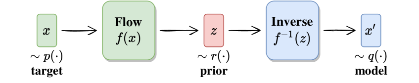
Figure 2: Using a flow to generate data $x^{\prime}$. Image adapted from [3]

We can construct a normalizing flow by composing multiple invertible functions $f_{i}$ so that $x\equiv\left[f_{k}\circ f_{k-1}\circ\cdots\circ f_{2}\circ f_{1}\right](z)$. In practice, the functions $f_{i}$ are usually implemented as coupling layers, which update an “active” subset of the variables, conditioned on the complimentary “frozen” variables [4, 5].

1.3 Affine Coupling Layers

A particularly useful template function for constructing our normalizing flows is the affine coupling layer [6, 2],

$$f(x_{1},x_{2}) =\left(e^{s(x_{2})}x_{1}+t(x_{2}),\,x_{2}\right),\quad\text{with}\quad\log J(x)=\sum_{k}\left[s(x_{2})\right]_{k}$$

$$f^{-1}(x^{\prime}_{1},x^{\prime}_{2}) =\left((x^{\prime}_{1}-t(x^{\prime}_{2}))e^{-s(x^{\prime}_{2})},\,x^{\prime}_{2}\right),\quad\text{with}\quad\log J(x^{\prime})=\sum_{k}-\left[s(x^{\prime}_{2})\right]_{k}$$

where $s(x_{2})$ and $t(x_{2})$ are of the same dimensionality as $x_{1}$ and the functions act element-wise on the inputs.

In order to effectively draw samples from the correct target distribution $p(\cdot)$, our goal is to minimize the error introduced by approximating $q(\cdot)\simeq p(\cdot)$. To do so, we use the (reverse) Kullback-Leibler (KL) divergence from Eq. 3, which is minimized when $p=q$.

$$D_{\mathrm{KL}}(q\|p) \equiv\int dyq(y)\left[\log q(y)-\log p(y)\right]$$ (3)

$$\simeq\frac{1}{N}\sum_{i=1}^{N}\left[\log q(y_{i})-\log p(y_{i})\right],\,\,\text{where}\,\,y_{i}\sim q$$ (4)

2 Trivializing Map

Ultimately, our goal is to evaluate expectation values of the form

$$\langle\mathcal{O}\rangle=\tfrac{1}{\mathcal{Z}}\int dx\,\mathcal{O}(x)e^{-S(x)}.$$ (5)

Using a normalizing flow, we can perform a change of variables $x=f(z)$, so Eq. 5 becomes

$$\langle\mathcal{O}\rangle =\frac{1}{\mathcal{Z}}\int dz\left|\det\left[J(z)\right]\right|\mathcal{O}(f(z))e^{-S(f(z))},\text{ where }J(z)=\frac{\partial f(z)}{\partial z}$$ (6)

$$=\frac{1}{\mathcal{Z}}\int dz\mathcal{O}(f(z))e^{-S(f(z))+\log|\det[J(z)]|}.$$ (7)

We require the Jacobian matrix, $J(z)$, to be:

1. Injective (1-to-1) between domains of integration

2. Continuously differentiable (or, differentiable with continuous inverse)

The function $f$ is a trivializing map [7] when $S(f(z))-\log\left|\det J(z)\right|=\text{const.}$, and our expectation value simplifies to

$$\langle\mathcal{O}\rangle=\frac{1}{\mathcal{Z}^{\ast}}\int dz\,\mathcal{O}(f(z)),\text{ where }\frac{1}{\mathcal{Z}^{\ast}}=\frac{1}{\mathcal{Z}}\exp(-\text{const.}).$$ (8)

3 Field Transformation HMC: fthmc

We can implement the trivializing map defined in Sec. 2 using a normalizing flow model. For conjugate momenta $\pi$, we can write the Hamiltonian as

$$H(z,\pi)=\frac{1}{2}\pi^{2}+S(f(z))-\log\left|\det J(f(z))\right|,$$ (9)

and the associated equations of motion as

$$\dot{z} =\frac{\partial H}{\partial\pi}=\pi$$ (10)

$$\dot{\pi} =-J(z)S^{\prime}(f(z))+\mathrm{tr}\left[J^{-1}\frac{d}{dz}J\right].$$ (11)

If we introduce a change of variables, $\pi=J(z)\rho=J(f^{-1}(x))\rho$ and $z=f^{-1}(x)$, the determinant of the Jacobian matrix reduces to $1$, and we obtain the modified Hamiltonian

$$\tilde{H}(x,\rho)=\frac{1}{2}\rho^{\dagger}\rho+S(x)-\log|\det J|.$$ (12)

As shown in Figure 3, we can use a field transformation, $f^{-1}:z\rightarrow x$ to perform HMC updates on the transformed variables $x$, and $f:x\rightarrow z$ to recover the physical target distribution.

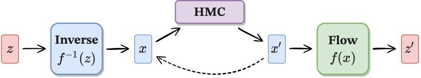
Figure 3: Normalizing flow with inner HMC block.

3.1 Hamiltonian Monte Carlo (HMC)

We describe the general procedure of the Hamiltonian Monte Carlo algorithm [8].

1. Introduce $v\sim\mathcal{N}(0,\mathbb{I}_{n})\in\mathbb{R}^{n}$ and write the joint distribution as

   $$p(x,v)=p(x)p(v)\propto e^{-S(x)}e^{-\frac{1}{2}v^{T}v}$$ (13)

2. Evolve the joint system $(\dot{x},\dot{v})$ according to Hamilton’s equations along $H=\text{const.}$ using the leapfrog integrator:

   $$\textbf{ (a.) }\tilde{v}\leftarrow v-\frac{\varepsilon}{2}\partial_{x}S(x)\quad\textbf{ (b.) }x^{\prime}\leftarrow x+\varepsilon\tilde{v}\quad\textbf{ (c.) }v^{\prime}\leftarrow\tilde{v}-\frac{\varepsilon}{2}\partial_{x}S(x^{\prime})$$ (14)

3. Accept or reject the proposal configuration using the Metropolis-Hastings test,

   $$x_{i+1}=\begin{cases}x^{\prime},\text{ with probability }A(x^{\prime}|x)\equiv\min\left\{1,\frac{p(x^{\prime})}{p(x)}\left|\frac{\partial x^{\prime}}{\partial x^{T}}\right|\right\}\\ x,\text{ with probability }1-A(x^{\prime}|x)\end{cases}$$ (15)

3.2 Volume Scaling

We use gauge equivariant coupling layers that act on plaquettes as the base layer for our network architecture. As in [5], these layers are composed of inner coupling layers which are implemented as stacks of convolutional layers. One advantage of using convolutional layers is that we can re-use the trained weights when scaling up to larger lattice volumes. Explicitly, when scaling up the lattice volume we can initialize the weights of our new network with the previously trained values. This approach has the advantage of requiring minimal retraining effort while being able to efficiently generate models on large lattice volumes.

4 Results

For traditional HMC, we see in Figure 4(a),4(b) that $Q\simeq 0$ for across all trajectories for both $8\times 8$ and $16\times 16$ lattice volumes. Conversely, we see in Figure 4(a),4(b) that the trained models are able to sample from multiple values of $Q$ for both the $8\times 8$ and $16\times 16$ volumes.

The results in Figure 5 took $\sim 4$ hours to train using a single A100 Nvidia GPU. The performance of the trained sampler is limited by the acceptance rate of the proposed configurations, which in turn, is ultimately limited by the computational resources used to train the model. Because of this, we would expect a continued improvement in performance with additional training. For this relatively simple proof of concept, we were able to demonstrate the usefuleness of our approach without requiring prohibitively large upfront training costs.

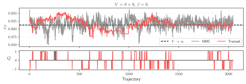
(a) The average plaquette $x_{P}$ and topological charge $Q$ histories for the trained model and HMC at $\beta=6$ with $V=8\times 8$.

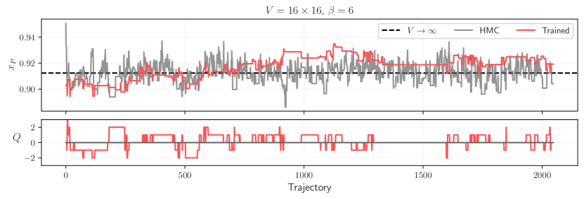
(b) The same model from Figure 4(a) used to generate configurations on $V=16\times 16$ lattice.

Figure 4: Comparison of lattice observables for both HMC and the trained model at $V=8\times 8$, and $V=16\times 16$.

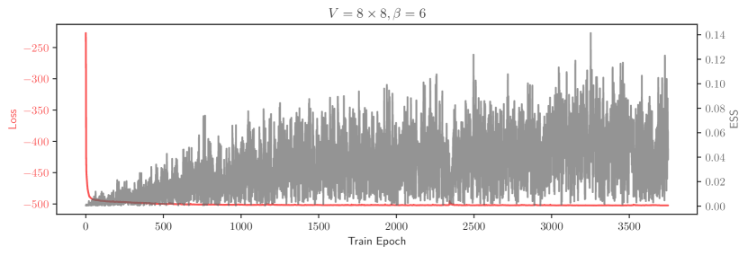
Figure 5: Loss and Effective Sample Size [9] (ESS) vs train epoch at $\beta=6$ on $V=8\times 8$ lattice.

5 Acknowledgments

This research was supported by the Exascale Computing Project (17-SC-20-SC), a collaborative effort of the U.S. Department of Energy Office of Science and the National Nuclear Security Administration. This research was performed using resources of the Argonne Leadership Computing Facility (ALCF), which is a DOE Office of Science User Facility supported under Contract DE_AC02–06CH11357. This work describes objective technical results and analysis. Any subjective views or opinions that might be expressed in the work do not necessarily represent the views of the U.S. DOE or the United States Government. Results presented in this research were obtained using the Python [10], programming language and its many data science libraries [11, 12, 13]

References

- [1] ALPHA collaboration, Critical slowing down and error analysis in lattice QCD simulations, Nucl. Phys. B 845 (2011) 93 [1009.5228].
- [2] D. Rezende and S. Mohamed, Variational inference with normalizing flows, in International conference on machine learning, pp. 1530–1538, PMLR, 2015.
- [3] L. Weng, Flow-based deep generative models, lilianweng.github.io/lil-log (2018) .
- [4] G. Kanwar, M.S. Albergo, D. Boyda, K. Cranmer, D.C. Hackett, S. Racanière et al., Equivariant flow-based sampling for lattice gauge theory, Phys. Rev. Lett. 125 (2020) 121601 [2003.06413].
- [5] M.S. Albergo, D. Boyda, D.C. Hackett, G. Kanwar, K. Cranmer, S. Racanière et al., Introduction to Normalizing Flows for Lattice Field Theory, arXiv e-prints (2021) [2101.08176].
- [6] L. Dinh, J. Sohl-Dickstein and S. Bengio, Density estimation using real NVP, CoRR abs/1605.08803 (2016) [1605.08803].
- [7] M. Lüscher, Trivializing Maps, the Wilson Flow and the HMC Algorithm, Communications in Mathematical Physics 293 (2009) 899–919.
- [8] M. Betancourt, A Conceptual Introduction to Hamiltonian Monte Carlo, arXiv e-prints (2017) arXiv:1701.02434 [1701.02434].
- [9] V. Elvira, L. Martino and C.P. Robert, Rethinking the Effective Sample Size, arXiv e-prints (2018) arXiv:1809.04129 [1809.04129].
- [10] G. Van Rossum and F.L. Drake Jr, Python Tutorial, Centrum voor Wiskunde en Informatica Amsterdam, The Netherlands (1995).
- [11] T.A. Caswell, M. Droettboom, J. Hunter, E. Firing, A. Lee, J. Klymak et al., matplotlib/matplotlib v3.1.0, May, 2019. 10.5281/zenodo.2893252.
- [12] C.R. Harris, K.J. Millman, S.J. van der Walt, R. Gommers, P. Virtanen, D. Cournapeau et al., Array programming with NumPy, Nature 585 (2020) 357.
- [13] F. Perez and B.E. Granger, IPython: A System for Interactive Scientific Computing, Computing in Science and Engineering 9 (2007) 21.