LeapfrogLayers: A Trainable Framework for Effective Topological Sampling

Abstract

We introduce LeapfrogLayers, an invertible neural network architecture that can be trained to efficiently sample the topology of a 2D $U(1)$ lattice gauge theory. We show an improvement in the integrated autocorrelation time of the topological charge when compared with traditional HMC, and look at how different quantities transform under our model. Our implementation is open source, and is publicly available on GitHub at github.com/saforem2/l2hmc-qcd.

1 Introduction

The main task in lattice field theory calculations is to evaluate integrals of the form

$$\langle\mathcal{O}\rangle=\int\left[\mathcal{D}\mathbf{x}\right]\mathcal{O}(\mathbf{x})p(\mathbf{x}),$$ (1)

for some normalized multivariate target distribution $p(\mathbf{x})=e^{-S(\mathbf{x})}/Z$. We can approximate the integral using Markov Chain Monte Carlo (MCMC) sampling techniques. This is done by sequentially generating a chain of configurations $\{\mathbf{x}_{1},\mathbf{x}_{2},\ldots\mathbf{x}_{N}\}$, with $\mathbf{x}_{i}$ occurring according to the stationary distribution $p(\mathbf{x})$, and averaging the value of the function $\mathcal{O}(\mathbf{x})$ over the chain

$$\overline{\mathcal{O}}=\frac{1}{N}\sum_{n=1}^{N}\mathcal{O}(\mathbf{x}_{n}).$$ (2)

Accounting for correlations between states in the chain, the sampling variance is given by

$$\sigmaup^{2}=\frac{\tau_{\mathcal{O}}^{\mathrm{int}}}{N}\sum_{n=1}^{N}\left[\mathcal{O}(\mathbf{x}_{n})-\overline{\mathcal{O}}\right]^{2}$$ (3)

where $\tau^{\mathrm{int}}_{\mathcal{O}}$ is the integrated autocorrelation time. This quantity can be interpreted as the additional time required for these induced correlations to become negligible.

While our main target for improved gauge field generation is full QCD, here we restrict our work to the simpler 2D U(1) pure-gauge lattice theory. There are already many efficient alternatives for simulating this particular theory (see e.g. [1] and references therein for a comparison), however scaling up to full QCD remains challenging. As the preferred method for full QCD, here HMC is our baseline for performance comparison. The method presented here can be extended to full QCD in a relatively straightforward manner, though the cost of training and efficiency are still open questions.

1.1 Charge Freezing

The ability to efficiently generate independent configurations is currently a major bottleneck for lattice simulations. The 2D U(1) gauge theory considered here has sectors of topological charge that become separated by large potential barriers for increasing $\beta$, similar to full QCD.

The theory is defined in terms of the link variables $U_{\mu}(x)=e^{ix}\in U(1)$ with $x\in[-\pi,\pi)$. Our target distribution is given by $p(\mathbf{x})\propto e^{-S_{\beta}(\mathbf{x})}$, where $S_{\beta}(\mathbf{x})$ is the Wilson action

$$S_{\beta}(\mathbf{x})=\beta\sum_{P}1-\cos{x_{P}},$$ (4)

defined in terms of the sum of the gauge variables around the elementary plaquette, $x_{P}\equiv x_{\mu}(n)+x_{\nu}(n+\hat{\mu})-x_{\mu}(n+\hat{\nu})-x_{\nu}(n)$, starting at site $n$ of the lattice, and $\sum_{P}$ denotes the sum over all such plaquettes. For a given lattice configuration, we can calculate the topological charge $Q\in\mathbb{Z}$ using

$$Q_{\mathbb{Z}}=\frac{1}{2\pi}\sum_{P}\left\lfloor x_{P}\right\rfloor,\text{ where }\left\lfloor x_{P}\right\rfloor\equiv x_{P}-2\pi\left\lfloor\frac{x_{P}+\pi}{2\pi}\right\rfloor.$$ (5)

As $\beta\rightarrow\infty$, we see that the value of $Q_{\mathbb{Z}}$ remains fixed for large durations of the simulation. This freezing can be quantitatively measured by introducing the tunneling rate (as measured between subsequent states in our chain $i$ and $i+1$ )

$$\overline{\delta Q}_{\mathbb{Z}}~{},~{}\mathrm{with}~{}~{}\delta Q_{\mathbb{Z},i}\equiv\left|Q_{\mathbb{Z},i+1}-Q_{\mathbb{Z},i}\right|\in\mathbb{Z},$$ (6)

which serves as a measure for how efficiently our chain is able to jump (tunnel) between sectors of distinct topological charge. From Figure 1, we can see that $\overline{\delta Q}_{\mathbb{Z}}\rightarrow 0$ as $\beta\rightarrow\infty$.

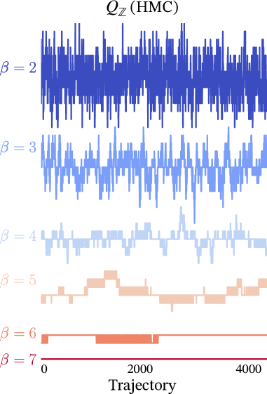
Figure 1: Illustration of the topological charge, $Q_{\mathbb{Z}}$, freezing as $\beta:{\color[rgb]{0.23046875,0.265625,0.75390625}{2}}\rightarrow{\color[rgb]{0.70703125,0.0234375,0.1484375}{7}}$ for traditional HMC.

2 Hamiltonian Monte Carlo (HMC)

The Hamiltonian Monte Carlo algorithm begins by introducing a fictitious momentum, $v$, for each coordinate variable, $x$, typically taken from an independent normal distribution. This allows us to write the joint target density of the $\xi\equiv(\mathbf{x},\mathbf{v})$ system as

$$p(\mathbf{x},\mathbf{v})=p(\mathbf{x})p(\mathbf{v})=e^{-S_{\beta}(\mathbf{x})}e^{-\mathbf{v}^{2}/2}=e^{-\mathcal{H}(\mathbf{x},\mathbf{v})}$$ (7)

where $\mathcal{H}(\xi)=\mathcal{H}(\mathbf{x},\mathbf{v})=S_{\beta}(\mathbf{x})+\frac{1}{2}\mathbf{v}^{2}$ is the Hamiltonian of the system. We use the leapfrog integrator to approximately numerically integrate Hamilton’s equations

$$\dot{\mathbf{x}}=\frac{\partial\mathcal{H}}{\partial\mathbf{v}}\quad\text{,}\quad\dot{\mathbf{v}}=-\frac{\partial\mathcal{H}}{\partial\mathbf{x}}$$ (8)

along iso-probability contours of $\mathcal{H}=\text{const.}$ from $\xi=(\mathbf{x},\mathbf{v})\rightarrow(\mathbf{x}^{\ast},\mathbf{v}^{\ast})=\xi^{\ast}$. The error in this integration is then corrected by a Metropolis-Hastings (MH) accept/reject step.

2.1 HMC algorithm with Leapfrog Integrator

1. Starting from $\mathbf{x}_{i}$, resample the momentum $\mathbf{v}_{i}\sim\mathcal{N}(0,\mathbbm{1})$ and construct the state $\xi=(\mathbf{x}_{i},\mathbf{v}_{i})$.

2. Generate a proposal configuration $\xi^{\ast}$ by integrating $\dot{\xi}$ along $\mathcal{H}=\mathrm{const.}$ for $N$ leapfrog steps. i.e.

   $$\xi\rightarrow\xi_{1}\rightarrow\ldots\rightarrow\xi_{N}\equiv\xi^{\ast},$$ (9)

   where a single leapfrog step $\xi_{i}\rightarrow\xi_{i+1}$ above consists of:

   $$\textbf{ (a.) }\mathbf{v}^{\prime}\leftarrow\mathbf{v}-\frac{\varepsilon}{2}\partial_{\mathbf{x}}S(\mathbf{x}),\quad\quad\textbf{ (b.) }\mathbf{x}^{\prime}\leftarrow\mathbf{x}+\varepsilon\mathbf{v}^{\prime},\quad\quad\textbf{ (c.) }\mathbf{v}^{\prime\prime}\leftarrow\mathbf{v}^{\prime}-\frac{\varepsilon}{2}\partial_{\mathbf{x}}S(\mathbf{x}).$$ (10)

3. At the end of the trajectory, accept or reject the proposal configuration $\xi^{\ast}$ using the MH test

   $$\mathbf{x}_{i+1}\leftarrow\begin{cases}\mathbf{x}^{\ast}\text{ with probability }A(\xi^{\ast}|\xi)\equiv\min\left\{1,\frac{p(\xi^{\ast})}{p(\xi)}\right\}\\ \mathbf{x}_{i}\text{ with probability }1-A(\xi^{\ast}|\xi).\end{cases}$$ (11)

An illustration of this procedure can be seen in Figure 2.

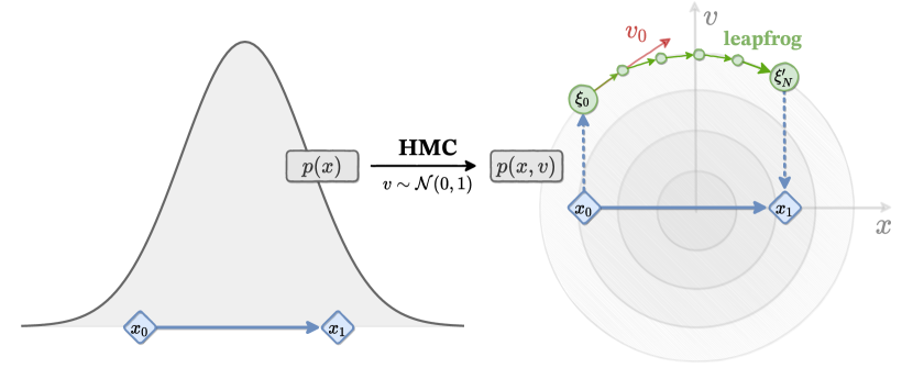
Figure 2: High-level overview of the HMC algorithm.

2.2 Issues with HMC

The HMC sampler is known to have difficulty traversing areas where the action is large. This makes it less likely for the system to go into low probability regions, and effectively bounds the system within potential barriers, resulting in poor performance for distributions which have multiple isolated modes. This is particularly relevant in the case of sampling topological quantities in lattice gauge models.

3 Generalizing HMC: LeapfrogLayers

In order to preserve the exact stationary distribution of the Markov Chain, our update must be explicitly reversible with a tractable Jacobian determinant. To simplify notation, we introduce two functions, $\Gamma$ $(\Lambda)$ to denote the $\mathbf{v}$ $(\mathbf{x})$ updates. As in HMC, we follow the general pattern of performing alternating updates of $\mathbf{v}$ and $\mathbf{x}$.

We can ensure the Jacobian is simple by splitting the $\mathbf{x}$ update into two parts and sequentially updating complementary subsets using a binary mask ${\color[rgb]{0,0.49609375,1}{m}}$ and its complement ${\color[rgb]{1,0.125,0.3203125}\bar{m}}$. As in [2], we introduce $d\sim\mathcal{U}(+,-)$, distributed independently of both $\mathbf{x}$ and $\mathbf{v}$, to determine the “direction” of our update. Here, we associate $+$ $(-)$ with the forward (backward) direction and note that running sequential updates in opposite directions has the effect of inverting the update. We denote the complete state by $\xi=(\mathbf{x},\mathbf{v},d)$, with target density given by $p(\xi)=p(\mathbf{x})p(\mathbf{v})p(d)$.

Explicitly, we can write this series of updates as

$$\textbf{(a.)}\,\,\,\mathbf{v}^{\prime}\leftarrow\Gamma^{\pm}\left[\mathbf{v};\,\zeta_{\mathbf{v}}\right]\hskip 80.0pt \textbf{(b.)}\,\,\,\mathbf{x}^{\prime}\leftarrow{\color[rgb]{0,0.49609375,1}{m}}\odot\mathbf{x}+{\color[rgb]{1,0.125,0.3203125}\bar{m}}\odot\Lambda^{\pm}[{\color[rgb]{1,0.125,0.3203125}x_{\bar{m}}};\zeta_{\bar{\mathbf{x}}}]$$

$$\textbf{(c.)}\,\,\mathbf{x}^{\prime\prime}\leftarrow{\color[rgb]{1,0.125,0.3203125}\bar{m}}\odot\mathbf{x}^{\prime}+{\color[rgb]{0,0.49609375,1}{m}}\odot\Lambda^{\pm}[{\color[rgb]{0,0.49609375,1}{x}_{m}};\zeta_{\mathbf{x}^{\prime}}]\quad \textbf{(d.)}\,\,\mathbf{v}^{\prime\prime}\leftarrow\Gamma^{\pm}[\mathbf{v}^{\prime},\zeta_{\mathbf{v}^{\prime}}]$$

where $\zeta_{\bar{\mathbf{x}}}=[{\color[rgb]{1,0.125,0.3203125}\bar{m}}\odot\mathbf{x},\mathbf{v}]$, $\zeta_{\mathbf{x}}=[{\color[rgb]{0,0.49609375,1}{m}}\odot\mathbf{x},\mathbf{v}]$ $(\zeta_{\mathbf{v}}=[\mathbf{x},\partial_{\mathbf{x}}S(\mathbf{x})])$ is independent of $\mathbf{x}$ $(\mathbf{v})$ and is passed as input to the update functions $\Lambda^{\pm}$ $(\Gamma^{\pm})$. The acceptance probability

$$A(\xi^{\ast}|\xi)=\min\left\{1,\frac{p(\xi^{\ast})}{p(\xi)}\mathcal{J}(\xi^{\ast},\xi)\right\}$$ (12)

now includes a Jacobian factor $\mathcal{J}(\xi^{\ast},\xi)$ which allows the inclusion of non-symplectic update steps. The Jacobian comes from the $v$ ($x$) scaling term in the $v$ ($x$) update, and is easily calculated.

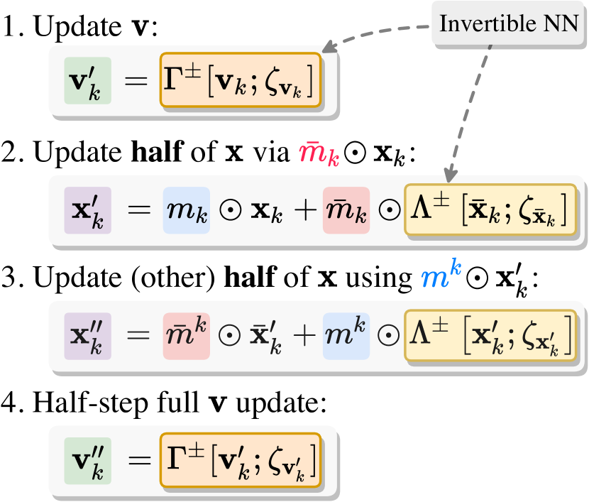
(a) Generalized leapfrog update.

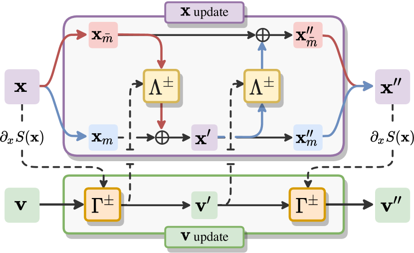
(b) Illustration of the data flow through a leapfrog layer.

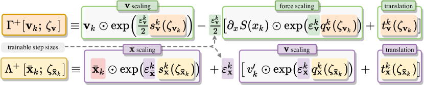
(c) Detailed view of the update functions $\Gamma^{+},\Lambda^{+}$ for the $k^{\mathrm{th}}$ leapfrog step.

Figure 3: Illustrations of the generalized leapfrog update. In Figure 3(a),  3(c), we denote $\bar{\mathbf{x}}_{k}={\color[rgb]{1,0.125,0.3203125}\bar{m}}\odot\mathbf{x}_{k}$.

3.1 Network Details

Normalizing flows [3] are an obvious choice for the structure of the update functions. These architectures are easily invertible while maintaining a tractable Jacobian determinant, and have also been shown to be effective at approximating complicated target distributions in high-dimensional spaces  [3, 2, 4, 5, 6, 7, 8, 9, 10, 11, 12, 13].

We maintain separate networks $\Gamma$, $\Lambda$ with identical architectures for updating $\mathbf{v}$ and $\mathbf{x}$, respectively. Without loss of generality, we describe below the details of the $\mathbf{x}$ update for the forward $(d=+)$ direction, $\Lambda^{+}[{\color[rgb]{1,0.125,0.3203125}x_{\bar{m}}};\zeta_{\bar{\mathbf{x}}}]$. For simplicity, we describe the data flow through a single leapfrog layer, which takes as input $\zeta_{\bar{\mathbf{x}}}=({\color[rgb]{1,0.125,0.3203125}x_{\bar{m}}},\mathbf{v})$. For the 2D $U(1)$ model, the gauge links are encoded as $[\cos(x),\sin(x)]$ for $x\in[-\pi,\pi]$. Explicitly,

$$h_{1} =\sigma\left(w_{x}\mathbf{x}+w_{v}\mathbf{v}+b_{1}\right)\quad\in\mathbb{R}^{n_{1}}$$ (13)

$$h_{2} =\sigma\left(w_{2}h_{1}+b_{2}\right)\hskip 37.59789pt\in\mathbb{R}^{n_{2}}$$ (14)

$$\vdots$$

$$h_{k} =\sigma\left(w_{k}h_{k-1}+b_{k-1}\right)\hskip 17.68875pt\in\mathbb{R}^{n_{k}}\Longrightarrow$$ (15)

$$\textbf{ (a.) }s_{x}=\lambda_{s}\tanh\left(w_{s}h_{k}+b_{s}\right); \quad\textbf{ (b.) }t_{x}=w_{t}h_{k}+b_{t};\quad\textbf{ (c.) }q_{x}=\lambda_{q}\tanh\left(w_{q}h_{k}+b_{q}\right);$$

where the outputs $s_{x},t_{x},q_{x}$ are of the same dimensionality as $\mathbf{x}$, and $\lambda_{s},\lambda_{q}$ are trainable parameters. These outputs are then used to update $\mathbf{x}$, as shown in Figure 3.

3.2 Training Details

Our goal in training the network is to find a sampler that efficiently jumps between different topological charge sectors. This can be done by constructing a loss function that maximizes the expected squared charge difference between the initial $(\xi)$ and proposal $(\xi^{\ast})$ configuration generated by the sampler. Explicitly, we define

$$\mathcal{L}_{\theta}(\xi^{\ast},\xi)=A(\xi^{\ast}|\xi)(Q^{\ast}_{\mathbb{R}}-Q_{\mathbb{R}})^{2}$$ (16)

where $Q_{\mathbb{R}}=\frac{1}{2\pi}\sum_{P}\sin x_{P}\in\mathbb{R}$ is a real-valued approximation of the usual (integer-valued) topological charge $Q_{\mathbb{Z}}\in\mathbb{Z}$. This ensures that our loss function is continuous which helps to simplify the training procedure. For completeness, the details of an individual training step are summarized in Sec 3.2.1.

3.2.1 Training Step

1. Resample $\mathbf{v}\sim\mathcal{N}(0,\mathbbm{1})$, $d\sim\mathcal{U}(+,-)$, and construct initial state $\xi=(\mathbf{x},\mathbf{v},\pm)$

2. Generate the proposal configuration $\xi^{\ast}$ by passing the initial state sequentially through $N_{\mathrm{LF}}$ leapfrog layers: $\xi\rightarrow\xi_{1}\rightarrow\ldots\rightarrow\xi_{N_{\mathrm{LF}}}=\xi^{\ast}$

3. Compute the Metropolis-Hastings acceptance $A(\xi^{\ast}|\xi)=\min\left\{1,\frac{p(\xi^{\ast})}{p(\xi)}\mathcal{J}(\xi^{\ast},\xi)\right\}$

4. Evaluate the loss function $\mathcal{L}\leftarrow\mathcal{L}_{\theta}(\xi^{\ast},\xi)$, and back propagate gradients to update weights

5. Evaluate Metropolis-Hastings criteria and assign the next state in the chain according to $\mathbf{x}_{t+1}\leftarrow\begin{cases}\mathbf{x}^{\ast}\text{ with prob. }A(\xi^{\ast}|\xi)\\ \mathbf{x}\text{ with prob. }1-A(\xi^{\ast}|\xi).\end{cases}$

3.3 Annealing

As an additional tool to help improve the quality of the trained sampler, we scale the action during the $N_{\mathrm{T}}$ training steps using the target distribution $p_{t}(x)\propto e^{-\gamma_{t}S(x)}$ for $t=0,1,\ldots,N_{\mathrm{T}}$. The scale factors, $\gamma_{t}$, monotonically increase according to an annealing schedule up to $\gamma_{N_{\mathrm{T}}}\equiv 1$, with $|\gamma_{i+1}-\gamma_{i}|\ll 1$. For $\gamma_{i}<1$, this helps to rescale (shrink) the energy barriers between isolated modes, allowing the training to experience sufficient tunneling even when the final distribution is difficult to sample.

4 Results

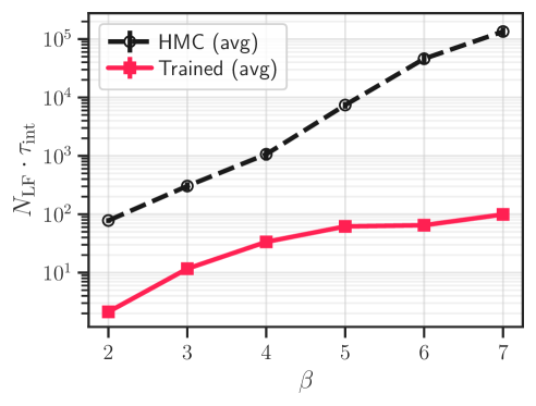
Figure 4: Estimated $\tau_{\mathrm{int}}^{\mathcal{Q}_{\mathbb{R}}}$ vs $\beta$.

We can measure the performance of our approach by comparing the integrated autocorrelation time against traditional HMC. We see in Figure 4 that our estimate of the integrated autocorrelation time is much shorter for the trained model across $\beta\in[2,7]$. To better understand how these transformations effect the HMC update, we can look at how various quantities change over the course of a trajectory, as shown in Figure 6. We see from the plot of $\mathcal{H}-\sum\log|\mathcal{J}|$ in Figure 6c that the trained sampler artificially increases the energy towards the middle of the trajectory. This is analogous to reducing the coupling $\beta$ during the trajectory, as can be seen in Figure 7(b). In particular, we can see that for $\beta=7$, the value of the plaquette at in the middle of the trajectory roughly corresponds to the expected value at $\beta=3$, indicated by the horizontal dashed line. This effective reduction in the coupling constant allows our sampler to mix topological charge values in the middle of the trajectory, before returning to the stationary distribution at the end, as can be seen in Figure 6(b). By looking at the variation in the average plaquette $\langle x_{P}-x^{\ast}_{P}\rangle$ over a trajectory for models trained at multiple values of beta we are able to better understand how our sampler behaves. This allows our trajectories to explore new regions of the target distribution which may have been previously inaccessible.

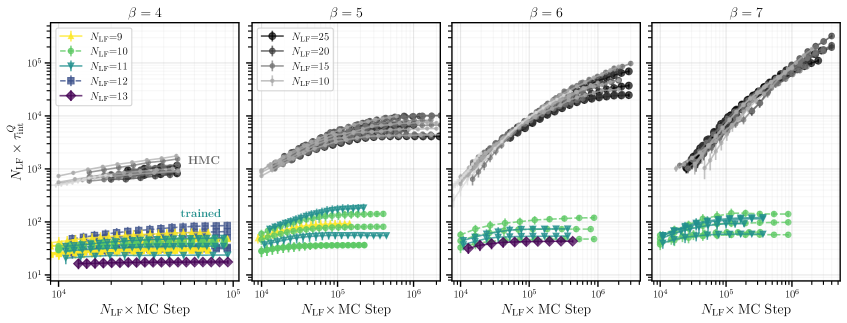
Figure 5: Comparison of the integrated autocorrelation time for trained models vs HMC with different trajectory lengths, $N_{\mathrm{LF}}$, at $\beta=4,5,6,7$ (left to right).

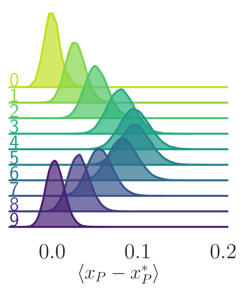
(a) Deviation in $x_{P}$.

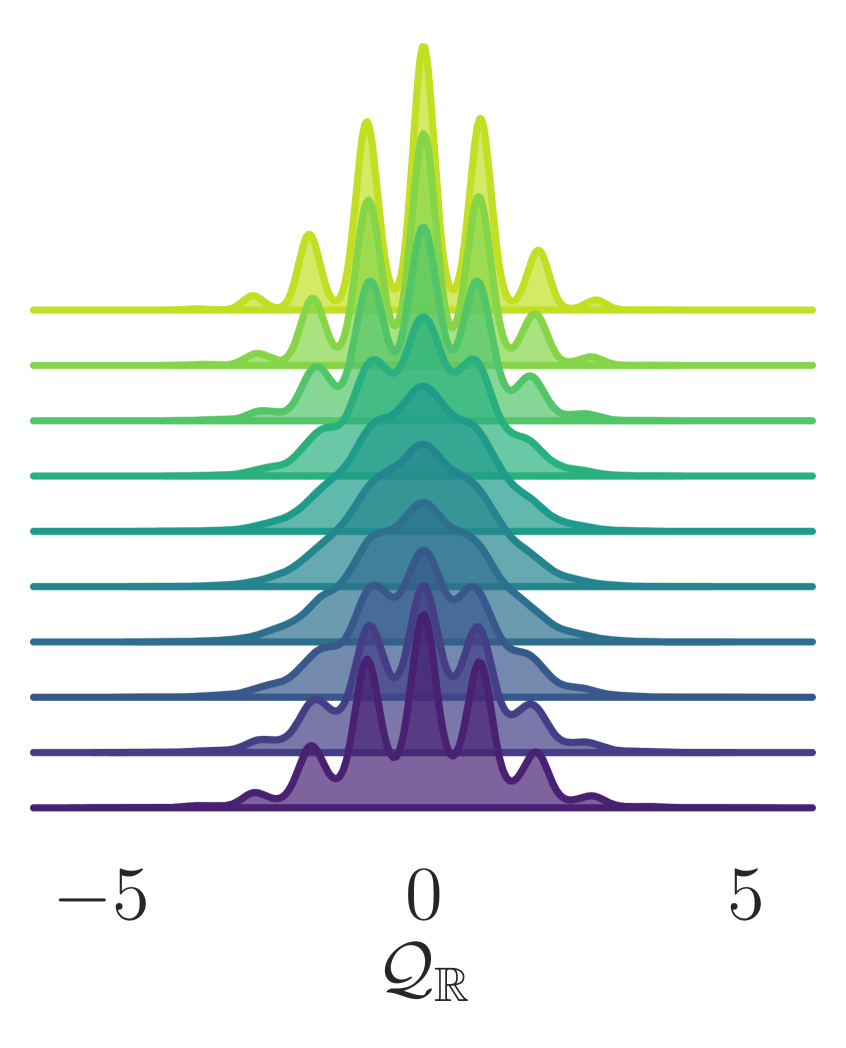
(b) Topological charge mixing $Q_{\mathbb{R}}$.

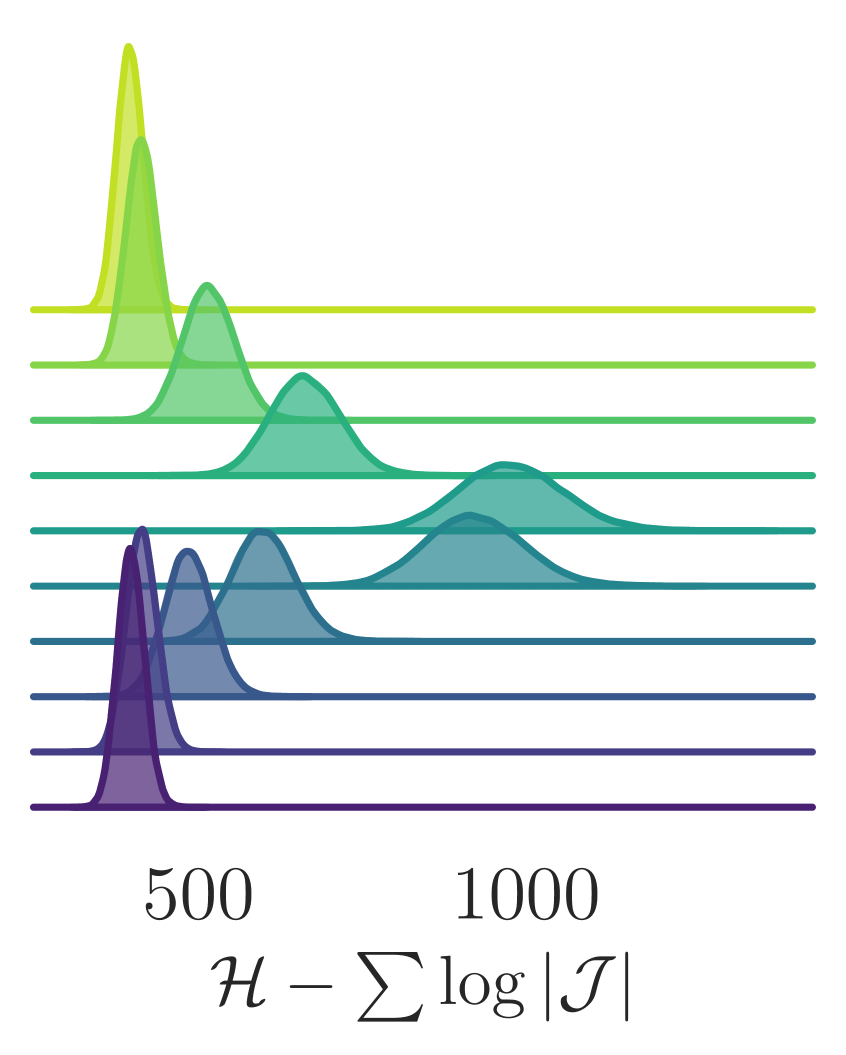
(c) Artificial influx of energy.

Figure 6: Evolution of different quantities over a single trajectory consisting of $N_{\mathrm{LF}}=10$ leapfrog steps.

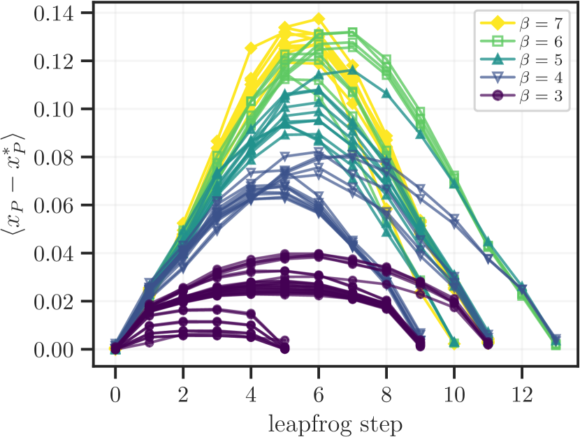
(a) The deviation of $x_{P}$ from the $V\rightarrow\infty$ limit, $x_{P}^{\ast}$.

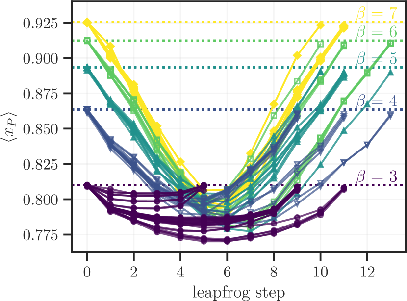
(b) Note $x^{\ast}_{P}$ is indicated by the horizontal dashed lines.

Figure 7: Plots showing how the plaquette varies over a single trajectory for models trained at $\beta={\color[rgb]{0.33984375,0.1171875,0.39453125}{3}},{\color[rgb]{0.30859375,0.390625,0.58984375}{4}},{\color[rgb]{0.171875,0.58984375,0.5703125}{5}},{\color[rgb]{0.3984375,0.796875,0.41015625}{6}},{\color[rgb]{0.9921875,0.90625,0.1484375}{7}}$.

5 Conclusion

In this work we have proposed a generalized sampling procedure for HMC that can be used for generating gauge configurations in the 2D $U(1)$ lattice model. We showed that our trained model is capable of outperforming traditional sampling techniques across a range of inverse coupling constants, as measured by the integrated autocorrelation time of the topological charge. By looking at the evolution of different quantities over the generalized leapfrog trajectory, we are able to gain insight into the mechanism driving this improved behavior.

6 Acknowledgments

This research was supported by the Exascale Computing Project (17-SC-20-SC), a collaborative effort of the U.S. Department of Energy Office of Science and the National Nuclear Security Administration. This research was performed using resources of the Argonne Leadership Computing Facility (ALCF), which is a DOE Office of Science User Facility supported under Contract DE_AC02–06CH11357. This work describes objective technical results and analysis. Any subjective views or opinions that might be expressed in the work do not necessarily represent the views of the U.S. DOE or the United States Government. Results presented in this research were obtained using the Python [14], programming language and its many data science libraries [15, 16, 17, 18].

References

- [1] T. Eichhorn and C. Hoelbling, Comparison of topology changing update algorithms, 2112.05188.
- [2] D. Levy, M.D. Hoffman and J. Sohl-Dickstein, Generalizing Hamiltonian Monte Carlo with Neural Networks, arXiv e-prints (2017) arXiv:1711.09268 [1711.09268].
- [3] L. Dinh, J. Sohl-Dickstein and S. Bengio, Density estimation using Real NVP, arXiv e-prints (2016) arXiv:1605.08803 [1605.08803].
- [4] S.-H. Li and L. Wang, Neural network renormalization group, Physical Review Letters 121 (2018) .
- [5] S. Foreman, Learning Better Physics: A Machine Learning Approach to Lattice Gauge Theory, Ph.D. thesis, The University of Iowa, 2019. 10.17077/etd.500b-30qp.
- [6] G. Kanwar, M.S. Albergo, D. Boyda, K. Cranmer, D.C. Hackett, S. Racanière et al., Equivariant flow-based sampling for lattice gauge theory, Phys. Rev. Lett. 125 (2020) 121601 [2003.06413].
- [7] J. Dumas, A. Wehenkel, D. Lanaspeze, B. Cornélusse and A. Sutera, You say normalizing flows i see bayesian networks, 2006.00866.
- [8] K.A. Nicoli, C.J. Anders, L. Funcke, T. Hartung, K. Jansen, P. Kessel et al., Estimation of Thermodynamic Observables in Lattice Field Theories with Deep Generative Models, 2007.07115.
- [9] D. Boyda, G. Kanwar, S. Racanière, D.J. Rezende, M.S. Albergo, K. Cranmer et al., Sampling using gauge equivariant flows, Phys. Rev. D 103 (2021) 074504 [2008.05456].
- [10] Z. Li, Y. Chen and F.T. Sommer, A neural network MCMC sampler that maximizes proposal entropy, 2010.03587.
- [11] M.S. Albergo, D. Boyda, D.C. Hackett, G. Kanwar, K. Cranmer, S. Racanière et al., Introduction to normalizing flows for lattice field theory, 2101.08176.
- [12] S. Foreman, T. Izubuchi, L. Jin, X.-Y. Jin, J.C. Osborn and A. Tomiya, HMC with Normalizing Flows, 2112.01586.
- [13] S. Foreman, X.-Y. Jin and J.C. Osborn, Deep Learning Hamiltonian Monte Carlo, 2105.03418.
- [14] G. Van Rossum and F.L. Drake Jr, Python Tutorial, Centrum voor Wiskunde en Informatica Amsterdam, The Netherlands (1995).
- [15] T.A. Caswell, M. Droettboom, J. Hunter, E. Firing, A. Lee, J. Klymak et al., matplotlib/matplotlib v3.1.0, May, 2019. 10.5281/zenodo.2893252.
- [16] C.R. Harris, K.J. Millman, S.J. van der Walt, R. Gommers, P. Virtanen, D. Cournapeau et al., Array programming with NumPy, Nature 585 (2020) 357.
- [17] Martín Abadi, Ashish Agarwal, Paul Barham, Eugene Brevdo, Zhifeng Chen, Craig Citro et al., “TensorFlow: Large-Scale Machine Learning on Heterogeneous Systems.”
- [18] F. Perez and B.E. Granger, IPython: A System for Interactive Scientific Computing, Computing in Science and Engineering 9 (2007) 21.