Reconstructing Orbits of Galaxies in Extreme Regions (ROGER) II: reliability of projected phase-space in our understanding of galaxy populations
Abstract
We connect galaxy properties with their orbital classification by analysing a sample of galaxies with stellar mass residing in and around massive and isolated galaxy clusters with mass at redshift . The galaxy population is generated by applying the semi-analytic model of galaxy formation sag on the cosmological simulation MultiDark Planck 2. We classify galaxies considering their real orbits (3D) and their projected phase-space position using the roger code (2D). We define five categories: cluster galaxies, galaxies that have recently fallen into a cluster, backsplash galaxies, infalling galaxies, and interloper galaxies. For each class, we analyse the colour, the specific star formation rate (sSFR), and the stellar age, as a function of the stellar mass. For the 3D classes, we find that cluster galaxies have the lowest sSFR, and are the reddest and the oldest, as expected from environmental effects. Backsplash galaxies have properties intermediate between the cluster and recent infaller galaxies. For each 2D class, we find an important contamination by other classes. We find it necessary to separate the galaxy populations in red and blue to perform a more realistic analysis of the 2D data. For the red population, the 2D results are in good agreement with the 3D predictions. Nevertheless, when the blue population is considered, the 2D analysis only provides reliable results for recent infallers, infalling galaxies and interloper galaxies.
keywords:
galaxies: clusters: general – galaxies: haloes – galaxies: kinematics and dynamics – methods: numerical – methods: analytical1 Introduction
Clusters of galaxies play a key role in galaxy evolution. In the last decades there have been several studies proving strong correlations between galaxy properties and their environment (see, for instance, Blanton et al. 2005; Martínez & Muriel 2006; Martínez et al. 2008). Properties such as colour (e.g. Balogh et al. 1999; Baldry et al. 2006; Coenda et al. 2018; Venhola et al. 2019), luminosity (e.g. Adami et al. 1998; Girardi et al. 2003; Coenda et al. 2006), star formation rate (e.g. Muzzin et al. 2012; Darvish et al. 2016; Coenda et al. 2019) and morphology (e.g. Dressler 1980; Bamford et al. 2009; Skibba et al. 2009; Kawinwanichakij et al. 2017) correlate with the galaxy position within the cluster.
Multiple physical mechanisms affect galaxies as they move through the deep potential well of a galaxy cluster. They can experience tidal stripping (e.g. Zwicky 1951; Gnedin 2003a; Villalobos et al. 2014), which, in turn, can induce a central star formation burst (Byrd & Valtonen, 2001) and bar instabilities (Łokas et al., 2016), remove stars from the galaxy (e.g. Ramos-Almendares et al. 2018), and truncate dark matter haloes (e.g. Gao et al. 2004; Limousin et al. 2009). In intermediate-density regions, gravitational phenomena such as galaxy-galaxy interactions and mergers can produce morphological transformations (Moore et al. 1996; Moore et al. 1998; Gnedin 2003b; Smith et al. 2015). Additionally, as galaxies move at high speed through the hot ionised gas of the intracluster medium, they can have a significant fraction of the cold gas removed through ram pressure stripping (e.g. Gunn & Gott 1972; Abadi et al. 1999; Book & Benson 2010; Steinhauser et al. 2016). On the other hand, the warm gas in the galaxy’s halo can also be removed, a process called starvation or strangulation (e.g. Larson et al. 1980; Balogh et al. 2000; McCarthy et al. 2008b; Bekki 2009; Peng et al. 2010; Bahé et al. 2013; Vijayaraghavan & Ricker 2015). The removal of these gaseous components ends up with red quenched galaxies.
In the hierarchical clustering scenario, clusters of galaxies are continuously accreting galaxies. In this process of falling, galaxies could undergo different physical processes that affect their star formation even before they reach the cluster, the so-called pre-processing (e.g. Balogh et al. 1999; Mihos 2004; Fujita 2004; McGee et al. 2009; De Lucia et al. 2012; Jaffé et al. 2012; Wetzel et al. 2013; Hou et al. 2014; Pallero et al. 2019). Most galaxies that fall into clusters come along filaments and experience different environmental effects than those falling from other directions (e.g. Martínez et al. 2016; Salerno et al. 2019). Moreover, galaxies that are members of a falling group will have different histories than those falling in isolation (e.g. McGee et al. 2009; De Lucia et al. 2012; Wetzel et al. 2013; Hou et al. 2014). Thus, from where and with whom a galaxy falls into a cluster matters.
In recent years, several authors began to study the outskirts of galaxy clusters (e.g. Mamon et al. 2004; Gill et al. 2005; Rines & Diaferio 2005; Aguerri & Sánchez-Janssen 2010; Mahajan et al. 2011; Muriel & Coenda 2014; Salerno et al. 2020; Benavides et al. 2021), finding not only infalling star-forming galaxies but also backsplash galaxies, i.e., galaxies whose orbits have taken them close to the cluster centre and are now beyond the virial radius. Having experienced different environmental effects during their evolution, it is expected that backsplash galaxies and galaxies infalling for the first time have different properties. Both should also present differences with respect to the population of passive galaxies in virial equilibrium inside the clusters.
It is not an easy task to differentiate observationally backsplash galaxies from infalling galaxies, although they are possibly distinguishable through kinematics (e.g. Gill et al. 2005; Pimbblet et al. 2006). Infalling galaxies starting from larger apocenters reach larger radial velocities at their pericenters (see fig. 9 of Mahajan et al. 2011). Recently, Haggar et al. (2020) studied the fraction of backsplash galaxies on the outskirts of clusters using hidrodynamical simulations. They found that the fraction of backsplash galaxies depends on the the dynamical state of a cluster, as dynamically relaxed clusters have a greater backsplash fraction. Muriel & Coenda (2014) explore the properties of galaxies in the outskirts of clusters, selecting low and high-velocity subsamples, according to their line-of-sight velocity relative to the cluster. They found that late-type galaxies in the low-velocity sample are systematically older, redder, and have formed fewer stars than galaxies in the high-velocity sample.
To understand how environmental processes affect galaxy properties, it is necessary to perform a good characterisation of the population of galaxies. Several authors classify galaxies around clusters using different criteria based on their position in the Projected Phase-Space Diagram (PPSD), which combines the projected cluster-centric distance with the line-of-sight velocity relative to the cluster (e.g. Mahajan et al. 2011; Oman et al. 2013; Muriel & Coenda 2014; Rhee et al. 2017). In de los Rios et al. (2021, hereafter dlR21), we present the code roger (Reconstructing Orbits of Galaxies in Extreme Regions) that relates the two-dimensional PPSD position (2D) of galaxies to their orbital classification (3D). The code uses three different machine learning techniques to classify galaxies in and around clusters according to their PPSD position. The main aim of this work is to understand how the inherent complexity of classifying galaxies according to their projected position affects the conclusions we draw about the connection between their observed properties (color, star formation rate, age) and their inferred dynamical state. To carry out this study, we use a sample of galaxy clusters generated by applying the semi-analytic model of galaxy formation sag (Cora et al., 2019) to a set of massive dark matter haloes extracted from the MultiDark Planck 2 cosmological simulation (Klypin et al., 2016). Firstly, we assign two orbital classifications to each galaxy, one given by their real orbit provided by the 3D phase-space and the other inferred from the PPSD through the code roger. Then, for a given galaxy class, we compare the distributions of galaxy properties (color, specific star formation rate, age) with respect to their stellar mass obtained for these two orbital classifications. Thus, we are able to evaluate the limits imposed by the 2D projections upon the conclusions that can be drawn from the observations. We also focus on the properties of galaxies classified according to their real orbits to find out how the environment affects galaxies when they cross the virial radius of a cluster.
This article is organised as follows. In section 2, we describe the sample of simulated galaxy clusters and their surroundings, the caracterisation of galaxies according to their orbits, and how we use the code roger to classify galaxies in the PPSD. The main results of the paper are presented in section 3, where we compare the properties of galaxies belonging to different dynamical classes and analyse the biases introduced by the 2D orbital classification. Finally, we present our conclusions and discussions in section 4.
2 Galaxy clusters and their surroundings
The sample of simulated galaxy clusters and of galaxies in their surroundings used throughout this work is generated by applying the semi-analytic model of galaxy formation and evolution sag (acronym of Semi-Analytic Galaxies; Cora et al. 2018) to the MultiDark Planck 2 cosmological simulation (mdpl2; Klypin et al. 2016). Here, we describe briefly the mdpl2 simulation, the sag model and the selection criteria used to construct the sample.
2.1 The mdpl2 cosmological simulation
The mdpl2 cosmological simulation is part of the MultiDark suite of cosmological simulations (Riebe et al., 2013; Klypin et al., 2016). This simulation counts with dark matter particles in a comoving cubic box of of side length, resulting in a particle mass . The adopted cosmology corresponds to a flat CDM model with , , and , in concordance with Planck measurements (Planck Collaboration et al., 2014, 2016). The simulation tracks the dynamical evolution of dark matter particles from the initial redshift using Gadget-2 (Springel, 2005). The outputs were stored into 126 snapshots between and .
Dark matter haloes in mdpl2 were identified using the phase-space halo finder Rockstar (Behroozi et al., 2013a), and the merger trees were constructed using ConsistentTrees (Behroozi et al., 2013b). The halo catalogues and merger trees used in this work are publicly available at the CosmoSim111https://www.cosmosim.org/cms/simulations/mdpl2/ and Skies & Universes 222http://skiesanduniverses.org/Simulations/MultiDark/ databases. They are the backbone of the semi-analytic model to generate the galaxy population.
2.2 The sag Model
The sag model originates from the semi-analytic model described in Springel et al. (2001). The latest version of the model is presented in Cora et al. (2018). The evolution of galaxy properties is followed by assigning one galaxy to each dark matter halo detected in the underlying dark matter simulation, and using the merger trees of haloes and subhaloes. sag includes radiative cooling of the hot halo gas in central and satellite galaxies, quiescent star formation in the gaseous disc, starbursts triggered by galaxy mergers and disc instabilities, which contributes to the formation of galaxy bulges (Lagos et al., 2008; Muñoz Arancibia et al., 2015; Gargiulo et al., 2015), a detailed treatment of chemical enrichment considering the contribution from stellar winds and different types of supernovae (Cora, 2006; Collacchioni et al., 2018), and feedback from supernova and active galactic nuclei (AGN). The modelling of the former takes into account an explicit dependence of the reaheated mass on redshift based on relations measured from full-physics hydrodynamical simulations; besides, gas from haloes is ejected and reincorporated later to avoid excess of star formation at high redshifts (Cora et al., 2018). The implementation of AGN feedback considers the growth of supermassive black holes in the centre of galaxies (Lagos et al., 2008; Cora et al., 2019).
Environmental effects like tidal stripping (TS) and ram pressure stripping (RPS) are also included in the model (Cora et al., 2018); they are particularly relevant for the interpretation of results obtained for galaxies classified according to their real orbits (3D classification; see Section 2.4). When Galaxies become satellites, they lose their hot gas in a gradual way by the action of RPS. The gradual stripping of the hot gas is modelled assuming a spherical isothermal density profile for the gas and following Font et al. (2008) and McCarthy et al. (2008a). When the ratio between the hot gas mass and the baryonic mass of a satellite galaxy decreases below , ram pressure can strip gas from the galaxy disc following the model of Tecce et al. (2010), where the stripping radius is calculated by using the Gunn & Gott (1972) condition. In any case, the ram pressure exerted on the gaseous components of satellite galaxies is estimated from an analytic fitting profile that recovers the ram pressure dependence on halo mass, halocentric distance and redshift using the information of the gas particle distribution in hydrodynamical simulations of groups and clusters of galaxies (Vega-Martínez et al., 2021). The mass and metals removed by RPS from both the hot gas halo and cold gas disc of the satellite are transferred to the hot gas of the galaxy identified as the central of the processed satellite (i.e. the intra-cluster/group medium), which is the central galaxy of the main host halo in most of the cases. sag also considers ejection of gas from the haloes as a result of supernovae feedback, but the ejected reservoir is not affected by RPS because of the uncertain physical interpretation of this galaxy component. The rest of the galaxy components (gaseous halo and disc, stellar disc and bulge) are also affected by TS but, in general, RPS dominates.
The modelling of these physical processes involves free parameters that are calibrated to a set of observed relations of galaxy properties by using the Particle Swarm Optimisation technique (Ruiz et al., 2015). The galaxy properties considered are the stellar mass functions at redshifts and , the star formation rate distribution function at , the fraction of mass in cold gas as a function of stellar mass at , and the relation between bulge mass and the mass of the central supermassive black hole at . The values of the set of free parameters that characterise the version of the model used here are given in table 1 of Cora et al. (2018), except the parameter that regulates the redshift dependence of the supernova feedback, which has been reduced to achieve a better agreement between simulated and observed values of the fraction of quenched galaxies as a function of stellar mass and halo mass (see fig. 11 in Cora et al. 2018 and the corresponding discussion).
It is worth noting that the calibration of the model takes into account orphan satellite galaxies, i.e., satellite galaxies whose dark matter substructure is not longer detected by the halo-finder. However, orphan galaxies are excluded from the sample considered for the analysis carried out in this work, as we did in dlR21. The orbits of orphan satellites are tracked by an orbital evolution model in a pre-processing step before applying sag and, thus, they are model dependent. Therefore, we only consider central galaxies and satellite galaxies that keep their dark matter substructure whose trajectory is well followed by the dark matter simulation.
2.3 Sample of simulated galaxies in and around clusters
The sample of clusters used in this work is the same used by dlR21. It contains 34 massive, relaxed and isolated galaxy clusters selected from the mdpl2-sag galaxy catalogue. Firstly, we select all haloes at redshift with mass that have no companion haloes within more massive than , where is the mass contained within the region of radius that encloses 200 times the critical density. These criteria exclude haloes undergoing a major merger, or interacting with a massive companion, which may affect galaxy orbits in the vicinity of galaxy clusters.
We also include in our analysis those galaxies residing in the surroundings of each selected cluster. For each cluster, we consider a region delimited by a cylinder elongated along the axis of the simulation box which is adopted as the line-of-sight direction, without loss of generality. This region includes the cluster galaxies, galaxies in the surroundings of the cluster, and interlopers. The latter are galaxies that appear in or around the cluster in projection but are unrelated to it; they constitute a major source of contamination in the PPSD. The dimensions of these cylinders are: a radius of , and a longitude in the axis that extends as far as to include all galaxies within , where is the galaxy peculiar velocity in the direction relative to the cluster, is the proper distance between the galaxy and the cluster centre in the direction, is the Hubble constant, and is the one dimensional velocity dispersion of the cluster. As shown by Munari et al. (2013), the value of is sensitive to the tracers used in its computation, i.e., dark matter particles or subhaloes. We use the values computed by dlR21. They measure the velocity dispersion of the clusters in our sample using as tracers those subhaloes that host a central galaxy (satellite galaxy) more massive than . This threshold in stellar mass was adopted to guarantee completeness in the sample of galaxies (Knebe et al., 2018). Below this mass limit, observed galaxy properties are not followed reliably.
2.4 Classification of galaxies in and around clusters based on their real orbits: 3D classification
We classify galaxies in and around clusters according to their real orbits in 3D using the same scheme as in dlR21. We consider the galaxies located within the region around each cluster of our sample and track their positions relative to the cluster centre in the successive outputs of the simulation. Thus, we define five orbital classes at redshift :
-
1.
Cluster galaxies (CL): These galaxies involve the central galaxy of the cluster, plus all galaxies that have been satellites of the cluster for more than . The latter have been either inside since they have been accreted by the cluster or they have crossed more than twice, or just once in their way in and earlier than ago. Most of them are located within , and a few are found temporarily outside in their orbital motion.
-
2.
Recent infallers (RIN): These galaxies are located within and have crossed this radius inwards only once in the last .
-
3.
Backsplash galaxies (BS): These galaxies are found outside and have crossed this radius exactly twice in their lifetimes, the first time on their way in, and the second on their way out of the cluster. According to this selection criterion, a RIN can become a BS in the future.
-
4.
Infalling galaxies (IN): These galaxies are in haloes that have negative radial velocity relative to the cluster centre and have never been within .
-
5.
Interlopers (ITL): These galaxies have never approached the cluster centre within , and they are found in haloes that are receding from the cluster. They are not related to the cluster but, as a result of projection effects, they can be confused with galaxies in classes iiv above in the PPSD.
Hereafter, we will refer to this classification of galaxies as 3D classification.
2.5 Classification of Galaxies based on the Projected Phase Space Diagram Using roger: 2D classification
In this section, we present a brief summary of the code roger presented in dlR21 and used in the present work to carry out the orbital classification of galaxies according to their projected phase space position.
The roger code is an automatic machine learning algorithm that determines the probability of each galaxy of belonging to the previously defined orbital classes using only their PPSD position. This code was presented as an R package333https://github.com/Martindelosrios/ROGER that can be installed and used directly from an R console.
To train and test roger, dlR21 used those galaxies within 33 out of the 34 regions around the massive, relaxed and isolated galaxy clusters in our sample (Section 2.3). With these galaxies they built two independent subsets, namely: a training-set used to train the machine learning models and a validation-set used to measure the performance of the models in each training epoch. In turn, the galaxies belonging to the remaining galaxy cluster were used as a testing set to measure the performance of the models after the full training. To avoid any over-fitting that may bias the present results, in this work we only use the galaxies corresponding to the testing and validation sets originally presented in dlR21.
Although roger has the possibility of using different machine learning techniques (random forest, k-nearest neighbours (KNN) and support vector machines), in the present work we use only the KNN implementation as was suggested by dlR21.
To perform an analysis of the galaxy properties that resembles what can be done in real observations, we compute for each galaxy of our sample its position in the PPSD. Phase space positions of galaxies relative to their parent cluster’s centre are computed by projecting the 3D cartesian coordinates of the galaxies in the mdpl2 box at redshift into the plane. Hereafter, the projected distance on this plane, , will be referred to as the 2D distance, and it will be quoted in units of unless otherwise specified. On the other hand, the axis velocity relative to the cluster, , is the line-of-sight velocity, and will be quoted in units of . Then, using the previously trained code roger (dlR21), we compute the probability of each galaxy to belong to each category.
As specified in dlR21, galaxies can be classified into the five classes defined in Section 2.4 from the probabilities computed by roger by choosing different thresholds. For instance, if the th galaxy has a probability of being a cluster galaxy, it will be classified as such only if the probability of being a cluster galaxy is the highest probability and if it is higher than the chosen threshold, i.e., . In this way, we can tune up the thresholds to end up with purer, although smaller, samples, or, conversely, end up with larger but more contaminated samples. To quantify the properties of the resulting classifications, dlR21 define the following statistics:
-
•
Sensitivity: the number of correct predictions of a given class in the resulting sample, divided by the total number of galaxies of that class in the validation-set.
-
•
Precision: the number of correctly predicted galaxies of a given class in the resulting sample, divided by the total number of galaxies of that class in the resulting sample.
| Class | CL | BS | RIN | IN | ITL |
|---|---|---|---|---|---|
| Real Number | |||||
| Predicted Number | |||||
| Threshold | |||||
| Precision | |||||
| Sensitivity |
Classifying galaxies by choosing different probability thresholds results in samples of different degree of sensitivity and contamination. We have probed different threshold values and kept those that, for each class, give purer samples (high precision) without loosing statistical power (high sensitivity). This exploration is equivalent to moving along the curves depicted in Fig. 5 of dlR21 which show the sensitivity and precision of the resulting samples for different probability threshold values. The usefulness of such curves can be understood by considering regions in the PPSD where different real classes coexist. For a galaxy located in one of these regions, the machine learning algorithm will predict similar probabilities for the coexisting classes, and hence, the galaxy will have two or more predicted probabilities of comparable magnitudes. If the probability thresholds are increased enough, such regions can be discarded, and, on the one hand, the contamination will decrease, while on the other hand, we pay the price of decreasing the sensitivity of the resulting samples. In the end, the trade-off between contamination and sensitivity is user dependent.
Table 1 shows the number of galaxies belonging to each orbital class, together with the thresholds values used for each class and their corresponding precision and sensitivity. As a result of this procedure, galaxies in our sample has two classifications: their (true) 3D classification based on their real orbit described in section 2.4, and a 2D classification, described in this section, based on the probabilities computed by roger and our selected threshold values.
Although with these threshold values, miss-classified galaxies are minimised, there is still some contamination in the final samples for each category. Hence, these miss-classified galaxies will introduce biases on the final properties of the different categories, that must be taken into account in any analysis. We remark that, although in the current work we focus the analysis on the results obtained using the roger code, these biases will be present in any study of galaxy properties that tries to make a dynamical classification from the PPSD positions since in real observations the full 3D orbits can not be determined. The analysis of the biases introduced by the 2D classifications in the statistical properties that characterise each category is the main contribution of this work and will be the main topic of the following sections.
3 Comparing properties of galaxies: 3D vs 2D classifications
In this section, we focus on the dependence on stellar mass of the colour, the specific star formation rate (sSFR), and the stellar age of galaxies, analysing the trends obtained for different orbital classes, and compare the results obtained from the 3D and 2D classifications. The results for the 3D classification are interpreted according to the environmental processes included in sag (Section 2.2).
3.1 Colour
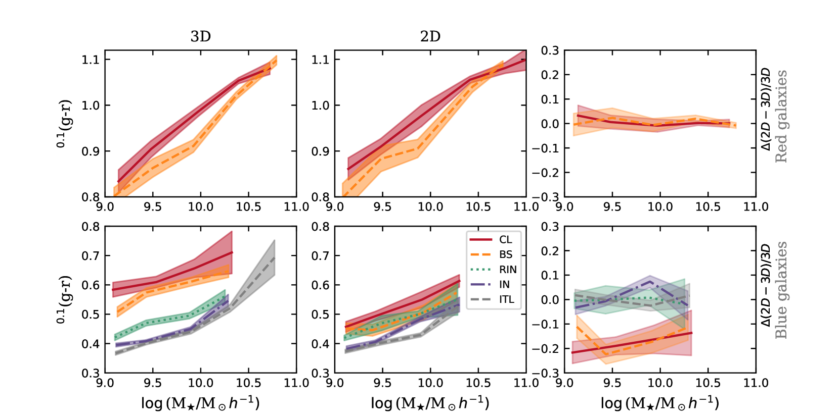
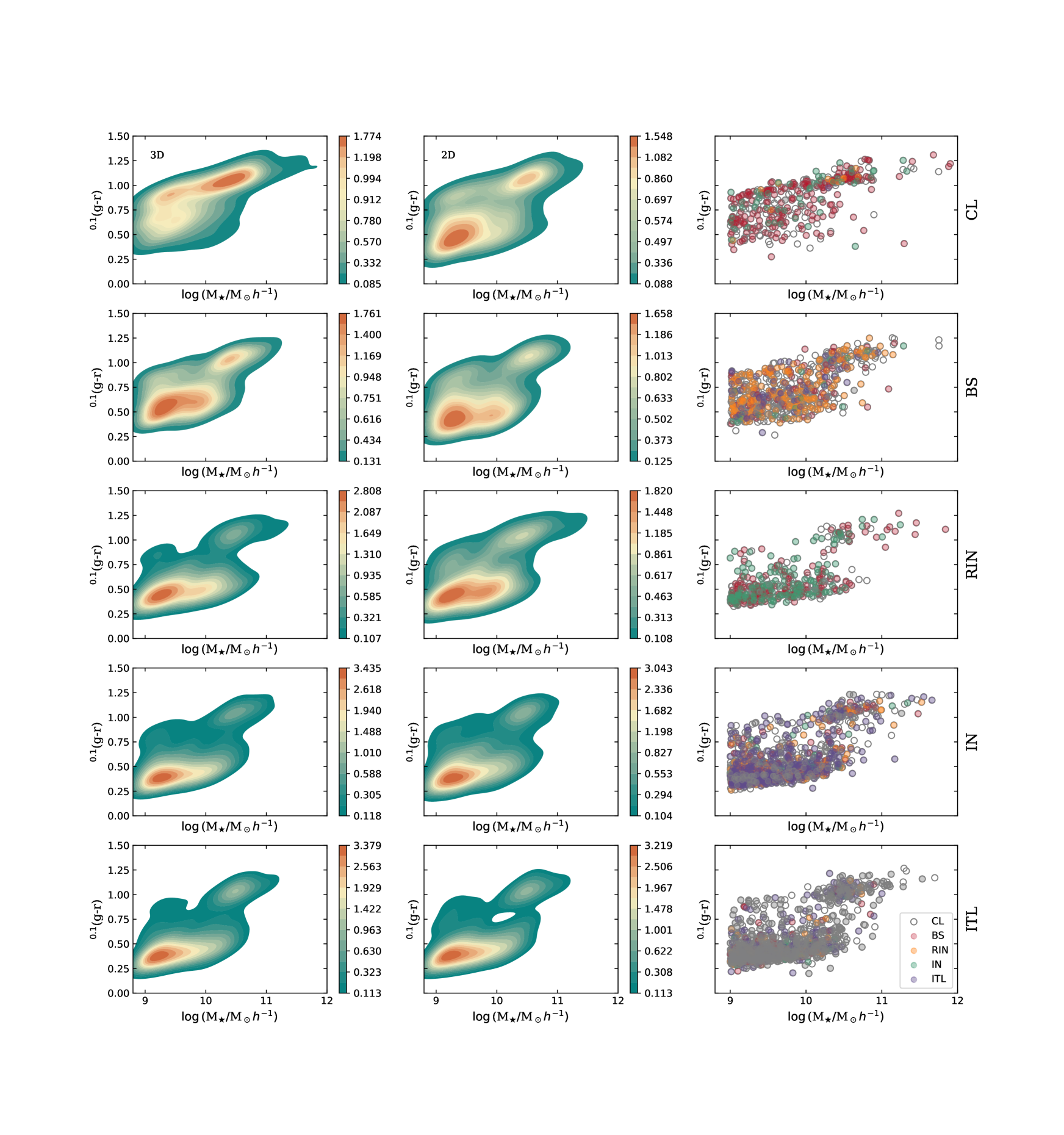
Fig. 1 shows the colour-stellar mass diagram for each galaxy class. We have adopted a band shift to a redshift for the colour to approximate the mean redshift of the main galaxy sample of SDSS (York et al., 2000). Left panels correspond to 3D classes, while central panels to 2D classes, classified out of their roger estimated probabilities. Different colours indicate the galaxy number density, from the lowest non-zero value (green) to the highest value (orange). On the other hand, right panels show in open circles the individual positions in the colour-mass diagram of the galaxies in the 3D category, where each circle is filled with a colour corresponding to the 2D classification. From top to bottom, we show CL, BS, RIN, IN and ITL galaxies, respectively; we observe a gradual increase of the blue population for both, 3D and 2D classes. For 3D classes, we see that the number of BS galaxies lying on the red sequence is lower than the corresponding number of CL galaxies, on one hand, and higher than the number of red RIN galaxies, on the other. If we consider the 2D classes, there is no clear difference in the galaxy distribution on the colour-stellar mass plane between BS and RIN. Right panels of Fig. 1 show how the colour-mass diagrams of the 2D classification are built up in terms of galaxies in the five 3D (real) classes. As can be seen from this figure, the most common miss-classifications occur between CL and RIN galaxies, and between BS and IN galaxies. Interlopers contaminate almost exclusively the IN class. It is worth mentioning that this behaviour was already pointed out by dlR21. These miss-classifications have immediate and important consequences for the 2D classes: CL galaxies appear to have a relevant blue cloud that is not real but a result of the contamination by bluer RIN galaxies; BS galaxies have a weaker red sequence due to contamination from bluer IN galaxies.
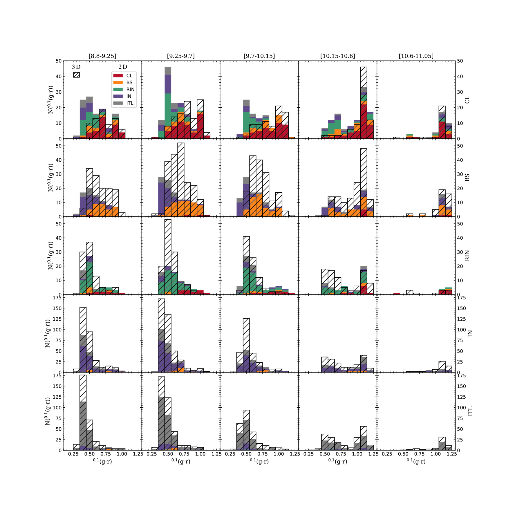
A more detailed analysis on how the 2D classes are made up out of the five 3D classes as a function of the stellar mass is shown in Fig. 2. In this figure, we split our samples of galaxies into five bins of stellar mass: , , , , and , and show the corresponding colour distributions. We observe a fictitious excess of blue galaxies in the 2D classes CL and BS over the whole mass range. In the case of CL galaxies, this blue excess is made up mostly by misclassified RIN galaxies. For BS galaxies, the main source of the excess are misclassified IN galaxies. In addition, we see that a large number of 3D BS galaxies are lost. They are either, classified as other class, or left out of the 2D classification as their computed probabilities of being BS do not exceed the chosen threshold. Fig. 2 warns about straightforward interpretations of observations when galaxies are classified according to their position in the PPSD. The blue population of galaxies classified as CL or BS will have a high degree of contamination thus affecting the conclusions that can be drawn. Nonetheless, we note that the red population of CL and BS galaxies are well recovered by roger. On the other hand, RIN, IN and ITL galaxies have a good agreement between the 3D and 2D types. It is worth emphasising that, although we are analysing the results obtained using the roger code, any code that classifies galaxies according to their PPSD position is likely to have similar biases.
In the light of Fig. 2, it is strongly recommended a separate analysis of the red sequence and the blue cloud whenever possible while studying galaxy properties in and around clusters. To separate our sample in red and blue populations, we consider a threshold linear in the logarithm of stellar mass, , adopted by Salerno et al. (2021, in preparation), based on the colour–stellar mass diagram for galaxies in the sag model at . In Fig. 3 we show the median value of the colour as a function of the stellar mass. Median colours are computed by splitting galaxies into the same stellar mass bins used in Fig. 2. We restrict to those bins containing at least ten galaxies. Shaded areas were computed using the bootstrap re-sampling technique. Given the low number of red galaxies in 2D types for the RIN, IN and ITL classes, we only analyse the properties of the red population of galaxies for CL and BS classes, hereafter.
From Fig. 3, we observe an increase of the median colour with increasing stellar mass for both the red and blue populations, when considering either the 3D or the 2D orbital classes (left and central panels, respectively). More specifically, for a fixed stellar mass, CL galaxies are systematically the reddest. In particular, for the red population of galaxies, there are no significant differences in colour between real and projected orbital types, as we show in the right panels of Fig. 3. We can see that the largest bin-to-bin differences are of the order of per cent and per cent, for CL and BS galaxies, respectively. For the blue population of the 3D types, there is a clear difference in colours among the galaxy types for a fixed stellar mass: CL galaxies are the reddest, followed by BS and RIN galaxies, in that order. IN and ITL galaxies are the bluest with small differences between them. However, we observe an important difference in colours between the 3D and 2D blue populations of classes CL and BS, being up to per cent for both, CL and BS galaxies. This is a consequence of the contamination by a the fictitious blue population discussed above (see Fig. 2). This discrepancy is not seen for the other classes, where the largest bin-to-bin differences are per cent for RIN and ITL galaxies, and per cent for IN galaxies.
The results shown in Fig. 3 strongly suggest that when studying CL and BS galaxies in observations, only their red populations can be reliably studied. On the other hand, studies of the blue population are reliable for RIN, IN, and ITL classes. Our samples do not allow for a reliable statistics of the red population of these latter classes.
3.2 Specific star formation rate and stellar age
Galaxy colours are a natural consequence of the evolution of the galaxy star formation rate, which also determines its average stellar age. Thus, we now analyse the sSFR and age of the red an blue galaxy populations, separately. As in Fig. 3, we split each sample in five stellar mass bins. In the light of the results in Sect. 3.1, the CL and BS galaxies have not been taken into account to analyse the blue populations of galaxies.
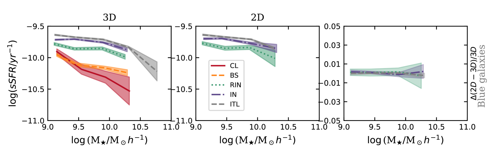
In Fig. 4, we compare the median values of the sSFR as a function of the stellar mass, for the blue population of galaxies in all five classes. We do not present the median values of sSFR for the red populations of galaxies because most of them have already ceased their star formation in their evolution. As those red galaxies have not formed new stars during the last time-step considered to calculate their sSFR, their null values of star formation rate can not be included in the current analysis. Moreover, the fraction of red galaxies featuring star formation is not large enough to do a robust comparison using them, as each stellar mass bin is filled with less than 10 galaxies.
As expected, the sSFR decreases with increasing stellar mass (e.g. Spindler et al. 2018; Belfiore et al. 2018; Coenda et al. 2019); this behaviour is observed independently of the galaxy class. For 3D classes, CL galaxies are the most passive systems, followed by BS types. RIN types are in a intermediate zone between BS and IN types. This explains the progressive redder colours displayed by these 3D classes, with IN being the bluest galaxies and CL the reddest ones.
If we focus only on the RIN, IN and ITL types, as suggested in the previous section, we do not observe a significant difference between the 3D and 2D classes, being the largest bin-to-bin differences of per cent for RIN and IN classes of galaxies, and per cent for ITL galaxies.
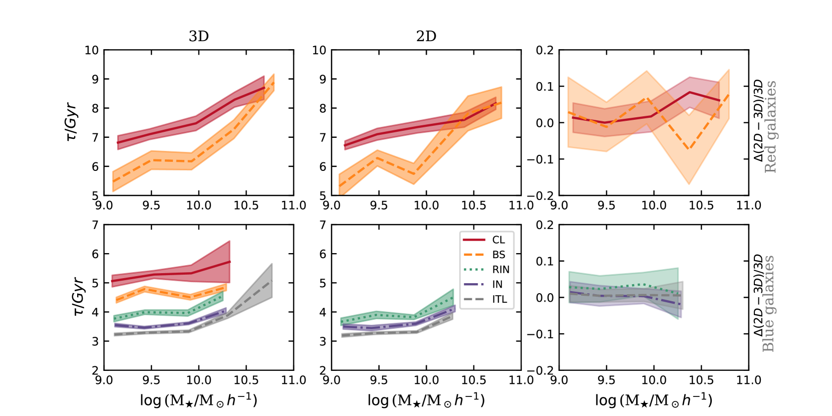
Finally, in Fig. 5, we analyse the median of stellar age as a function of the stellar mass. For the red sub-sample, CL galaxies are systematically the oldest. Only the highest stellar mass bin shows that BS and CL galaxies have similar stellar ages. The 2D trends are consistent with the 3D predictions. The bin-to-bin comparison shows that the differences between 2D and 3D are lower than per cent and almost consistent with zero considering the large errors. For the blue sub-sample of 3D types, CL galaxies are clearly the oldest ones followed by BS, RIN, IN and ITL galaxies, in that order. It is interesting to note that blue CL and BS galaxies differ significantly in in contrast to their similarity regarding colour or sSFR. For 2D types, we observe the same behaviour for RIN, IN and ITL types. The largest difference between 3D and 2D classes occurs for RIN galaxies, with a maximum value of per cent, while the largest difference for IN and ITL galaxies is per cent and per cent, respectively.
4 Discussion and Conclusions
In this paper we perform a comparison of properties of galaxies around massive and isolated clusters galaxies at , using a sample of galaxies generated from the combination of the semi-analytic model of galaxy formation (sag) and the MultiDark Planck 2 simulation (MDPL2). We track the orbit of the galaxies in our sample to define five galaxy classes: cluster galaxies (CL), galaxies that have recently fallen into a cluster (RIN), backsplash galaxies (BS), infalling galaxies (IN), and interlopers (ITL).
Since only galaxy positions in PPSD are accessible, different methods have been proposed to link these positions with orbits (e.g. the inversion of the Jeans equation, Binney & Mamon 1982; Natarajan & Kneib 1996; Biviano & Katgert 2004). We use the probabilities computed by roger, to make the best use of the PPSD information and classify our sample of galaxies into the five classes mentioned above. We choose different thresholds values for each class to minimise the overlapping regions in the projected phase-space and hence end with more pure samples. We analyse a number of galaxy properties: colour, the sSFR and the stellar age, as a function of the stellar mass, and consider separately red and blue sub-samples of galaxies for both the 3D classes (classified according to their real orbits) and the 2D classes (classified with roger).
Environmental effects inherent to galaxy clusters are clearly evident when focusing on the properties (colour, specific star formation rate, age) of 3D classes. Our results show that, for the red population and at fixed stellar mass, galaxies in clusters are redder and older than BS galaxies. For the blue population, CL galaxies are the reddest, the oldest and have the lowest specific star formation rate. When a galaxy dives into a cluster for the first time, environmental quenching onsets and the galaxy’s stellar population gets older and redder in comparison to galaxies external to the cluster. The action of environmental effects is even stronger for BS galaxies as they have travelled longer inside the cluster. However, they are not yet as red, old and with the star formation as quenched as the cluster galaxies that have experienced the environmental effects for a longer period, i.e., CL galaxies. Infalling and interlopers galaxies are quite similar; these are forming stars, are blue and have young stellar populations.
We interpret the trends depicted by galaxies classified according to their real orbits taking into account the modelling of environmental effects implemented in sag (see Section 2.2). Galaxies defined as satellites by the halo finder are affected by gradual removal of hot halo gas and cold gas disc by RPS. While most of CL galaxies are within the virial radius of the cluster, there are galaxies identified as satellites by the halo finder that reside at a further clustercentric distance. Hence, not only CL galaxies are affected by such processes but BS, RIN and IN galaxies could also feel the action of RPS when approaching the cluster. Therefore, galaxies that have dived for the first time into the cluster in the last 2 Gyr (RIN) already have signatures of the environmental quenching in their star formation rate (Fig. 4) and are redder than IN galaxies (Fig. 3). However, in the outskirts of clusters, the values of ram pressure are low, of the order of (see fig. 1 of Vega-Martínez et al. 2021).
When a satellite galaxy crosses the virial radius of a host halo and approaches the cluster centre, it is affected by increasing values of ram pressure, not only because ram pressure is higher in the inner regions of the cluster but also because of the build-up of the intra-cluster medium density over time as the satellite’s orbit evolves. At , most of satellite galaxies are already experiencing medium-level ram pressure (i.e., ) and, at , those satellites located within feel strong-level ram pressure, i.e., (Tecce et al. 2010; Vega-Martínez et al. 2021). The most important effect of RPS is the gradual removal of the hot gas component of satellite galaxies. The mass stripped by ram pressure is larger for less massive satellites, being the the cumulative stripped hot gas fractions of the order of per cent for low-mas satellites () and per cent for high-mas ones (; see fig. 14 of Cora et al. 2018). The lost of cold gas by RPS is an order of magnitude lower because the cold gas disc is shielded by the hot gas halo during most of the galaxy lifetime. Hence, the final effect of RPS is the reduction of the gas cooling rate which derives in the quenching of the star formation rate, which in turn is reflected in the colours and average ages of satellites.
It is clear then that the sSFR and colour is more affected the longer a galaxy is in a cluster, giving rise to the progressive quenching and reddening manifested by ITL, IN, RIN, BS and CL galaxies. A single excursion in and out of a cluster (BS) quenches star formation in a significant way. These results are in agreement with Lotz et al. (2019). Thus, with only one passage close to the centre of the cluster, galaxy colour is strongly affected, as suggested by the comparison between BS and RIN.
By focusing on the 2D classes, we see an important contamination over the projected populations: there are miss-classifications between CL and RIN galaxies, and BS and IN galaxies. Interlopers contaminate almost exclusively the IN class. These miss-classifications have significant consequences for the 2D classes: CL galaxies appear to have an exceptional blue cloud that is not real but a result of the contamination by bluer RIN galaxies; BS galaxies have a weaker red sequence due to contamination from bluer IN galaxies. This degree of contamination considerably affects the conclusions that can be deduced. From our results, we consider that it is necessary to separate the red and blue galaxy populations to perform a more realistic analysis of observational data. Reliable results can be obtained for red CL and BS galaxies, and for blue RIN and IN galaxies. Interlopers are not affected significantly by contamination. We recall that the red population of RIN, IN and ITL galaxies has not been analysed due to the low number of galaxies, however, these classes should not be discarded in future studies.
From the observational point of view, Muriel & Coenda (2014) explore several properties of early and late-types galaxies, defined in terms of their concentration index, in the outskirts of clusters. They select galaxies with projected distances in the range from a sample of X-ray selected clusters (Coenda & Muriel 2009; Muriel & Coenda 2014). They distinguish between low velocity (), and high velocity () galaxies. They find evidence that, for a fixed stellar mass, late-type low-velocity galaxies have formed less stars in the last 3 Gyr, are redder and older, than their high-velocity counterparts. In terms of their PPSD position, we can qualitatively associate high-velocity galaxies with the IN class, and the low-velocity galaxies with the BS class. Since each colour branch is also associated to a different galaxy morphology, i.e., late-type galaxies are associated to the blue cloud, whereas early-types are located in the red sequence in the colour-magnitude diagram (e.g. Conselice 2006), thus, the results of Muriel & Coenda (2014) are consistent with the results presented in this paper.
There are some works in the literature that compare the properties of galaxies classified according to their position in the projected phase-diagram (e.g. Biviano et al. 2002; Oman et al. 2013; Muzzin et al. 2014; Lotz et al. 2019; Lotz et al. 2021) but they are a few. However, there is effort to achieve a good separation of the galaxies in the phase-space diagram (e.g. Mahajan et al. 2011; Rhee et al. 2017; Jaffé et al. 2018). Based on the results shown here, we will apply the roger code to a real sample of galaxy clusters in a forthcoming paper to shed light on the properties of galaxies in the surroundings of galaxy clusters.
Acknowledgements
The authors thank the referee, Andrea Biviano, for his comments and suggestions that improved the paper. This paper has been partially supported with grants from Consejo Nacional de Investigaciones Científicas y Técnicas (CONICET, PIP 11220130100365CO) Argentina, the Agencia Nacional de Promoción Científica y Tecnológica (PICT 2016-1975), Argentina, and Secretaría de Ciencia y Tecnología, Universidad Nacional de Córdoba, Argentina. MdlR acknowledges financial support from the Comunidad Autónoma de Madrid through the grant SI2/PBG/2020-00005 and FAPESP through the process 2019/08852-2. SAC acknowledges funding from Consejo Nacional de Investigaciones Científicas y Técnicas (CONICET, PIP-0387), Agencia Nacional de Promoción de la Investigación, el Desarrollo Tecnológico y la Innovación (Agencia I+D+i, PICT-2018-03743), and Universidad Nacional de La Plata (G11-150), Argentina. CVM acknowledges financial support from the Max Planck Society through a Partner Group grant.
The CosmoSim database used in this paper is a service by the Leibniz-Institute for Astrophysics Potsdam (AIP). The authors gratefully acknowledge the Gauss Centre for Supercomputing e.V. (www.gauss-centre.eu) and the Partnership for Advanced Supercomputing in Europe (PRACE, www.prace-ri.eu) for funding the MultiDark simulation project by providing computing time on the GCS Supercomputer SuperMUC at Leibniz Supercomputing Centre (LRZ, www.lrz.de).
Data availability
roger data underlying this article are available in Github at https://github.com/Martindelosrios/ROGER and in zenodo at https://zenodo.org/badge/latestdoi/224241400. The raw data of the semi-analytic model of galaxy formation sag will be shared on reasonable request to the corresponding author.
References
- Abadi et al. (1999) Abadi M. G., Moore B., Bower R. G., 1999, MNRAS, 308, 947
- Adami et al. (1998) Adami C., Biviano A., Mazure A., 1998, A&A, 331, 439
- Aguerri & Sánchez-Janssen (2010) Aguerri J. A. L., Sánchez-Janssen R., 2010, A&A, 521, A28
- Bahé et al. (2013) Bahé Y. M., McCarthy I. G., Balogh M. L., Font A. S., 2013, MNRAS, 430, 3017
- Baldry et al. (2006) Baldry I. K., Balogh M. L., Bower R. G., Glazebrook K., Nichol R. C., Bamford S. P., Budavari T., 2006, MNRAS, 373, 469
- Balogh et al. (1999) Balogh M. L., Morris S. L., Yee H. K. C., Carlberg R. G., Ellingson E., 1999, ApJ, 527, 54
- Balogh et al. (2000) Balogh M. L., Navarro J. F., Morris S. L., 2000, ApJ, 540, 113
- Bamford et al. (2009) Bamford S. P., et al., 2009, MNRAS, 393, 1324
- Behroozi et al. (2013a) Behroozi P. S., Wechsler R. H., Wu H.-Y., 2013a, ApJ, 762, 109
- Behroozi et al. (2013b) Behroozi P. S., Wechsler R. H., Wu H.-Y., Busha M. T., Klypin A. A., Primack J. R., 2013b, ApJ, 763, 18
- Bekki (2009) Bekki K., 2009, MNRAS, 399, 2221
- Belfiore et al. (2018) Belfiore F., et al., 2018, MNRAS, 477, 3014
- Benavides et al. (2021) Benavides J. A., et al., 2021, Nature Astronomy,
- Binney & Mamon (1982) Binney J., Mamon G. A., 1982, MNRAS, 200, 361
- Biviano & Katgert (2004) Biviano A., Katgert P., 2004, A&A, 424, 779
- Biviano et al. (2002) Biviano A., Katgert P., Thomas T., Adami C., 2002, A&A, 387, 8
- Blanton et al. (2005) Blanton M. R., Eisenstein D., Hogg D. W., Schlegel D. J., Brinkmann J., 2005, ApJ, 629, 143
- Book & Benson (2010) Book L. G., Benson A. J., 2010, ApJ, 716, 810
- Byrd & Valtonen (2001) Byrd G., Valtonen M., 2001, AJ, 121, 2943
- Coenda & Muriel (2009) Coenda V., Muriel H., 2009, A&A, 504, 347
- Coenda et al. (2006) Coenda V., Muriel H., Donzelli C. J., Quintana H., Infante L., García Lambas D., 2006, AJ, 131, 1989
- Coenda et al. (2018) Coenda V., Martínez H. J., Muriel H., 2018, MNRAS, 473, 5617
- Coenda et al. (2019) Coenda V., Mast D., Martínez H. J., Muriel H., Merchán M. E., 2019, A&A, 621, A98
- Collacchioni et al. (2018) Collacchioni F., Cora S. A., Lagos C. D. P., Vega-Martínez C. A., 2018, MNRAS, 481, 954
- Conselice (2006) Conselice C. J., 2006, MNRAS, 373, 1389
- Cora (2006) Cora S. A., 2006, MNRAS, 368, 1540
- Cora et al. (2018) Cora S. A., et al., 2018, MNRAS, 479, 2
- Cora et al. (2019) Cora S. A., Hough T., Vega-Martínez C. A., Orsi Á. A., 2019, MNRAS, 483, 1686
- Darvish et al. (2016) Darvish B., Mobasher B., Sobral D., Rettura A., Scoville N., Faisst A., Capak P., 2016, ApJ, 825, 113
- De Lucia et al. (2012) De Lucia G., Weinmann S., Poggianti B. M., Aragón-Salamanca A., Zaritsky D., 2012, MNRAS, 423, 1277
- Dressler (1980) Dressler A., 1980, ApJ, 236, 351
- Font et al. (2008) Font A. S., Bower R. G., McCarthy I. G., et al. 2008, MNRAS, 389, 1619
- Fujita (2004) Fujita Y., 2004, PASJ, 56, 29
- Gao et al. (2004) Gao L., White S. D. M., Jenkins A., Stoehr F., Springel V., 2004, MNRAS, 355, 819
- Gargiulo et al. (2015) Gargiulo I. D., et al., 2015, MNRAS, 446, 3820
- Gill et al. (2005) Gill S. P. D., Knebe A., Gibson B. K., 2005, MNRAS, 356, 1327
- Girardi et al. (2003) Girardi M., Rigoni E., Mardirossian F., Mezzetti M., 2003, A&A, 406, 403
- Gnedin (2003a) Gnedin O. Y., 2003a, ApJ, 582, 141
- Gnedin (2003b) Gnedin O. Y., 2003b, ApJ, 589, 752
- Gunn & Gott (1972) Gunn J. E., Gott J. R. I., 1972, ApJ, 176, 1
- Haggar et al. (2020) Haggar R., Gray M. E., Pearce F. R., Knebe A., Cui W., Mostoghiu R., Yepes G., 2020, MNRAS, 492, 6074
- Hou et al. (2014) Hou A., Parker L. C., Harris W. E., 2014, MNRAS, 442, 406
- Jaffé et al. (2012) Jaffé Y. L., Poggianti B. M., Verheijen M. A. W., Deshev B. Z., van Gorkom J. H., 2012, ApJL, 756, L28
- Jaffé et al. (2018) Jaffé Y. L., et al., 2018, MNRAS, 476, 4753
- Kawinwanichakij et al. (2017) Kawinwanichakij L., et al., 2017, ApJ, 847, 134
- Klypin et al. (2016) Klypin A., Yepes G., Gottlöber S., Prada F., Heß S., 2016, MNRAS, 457, 4340
- Knebe et al. (2018) Knebe A., et al., 2018, MNRAS, 474, 5206
- Lagos et al. (2008) Lagos C. d. P., Cora S. A., Padilla N. D., 2008, MNRAS, 388, 587
- Larson et al. (1980) Larson R. B., Tinsley B. M., Caldwell C. N., 1980, ApJ, 237, 692
- Limousin et al. (2009) Limousin M., Sommer-Larsen J., Natarajan P., Milvang-Jensen B., 2009, ApJ, 696, 1771
- Łokas et al. (2016) Łokas E. L., Ebrová I., del Pino A., Sybilska A., Athanassoula E., Semczuk M., Gajda G., Fouquet S., 2016, ApJ, 826, 227
- Lotz et al. (2019) Lotz M., Remus R.-S., Dolag K., Biviano A., Burkert A., 2019, MNRAS, 488, 5370
- Lotz et al. (2021) Lotz M., Dolag K., Remus R.-S., Burkert A., 2021, MNRAS, 506, 4516
- Mahajan et al. (2011) Mahajan S., Mamon G. A., Raychaudhury S., 2011, MNRAS, 416, 2882
- Mamon et al. (2004) Mamon G. A., Sanchis T., Salvador-Solé E., Solanes J. M., 2004, A&A, 414, 445
- Martínez & Muriel (2006) Martínez H. J., Muriel H., 2006, MNRAS, 370, 1003
- Martínez et al. (2008) Martínez H. J., Coenda V., Muriel H., 2008, MNRAS, 391, 585
- Martínez et al. (2016) Martínez H. J., Muriel H., Coenda V., 2016, MNRAS, 455, 127
- McCarthy et al. (2008a) McCarthy I. G., Frenk C. S., Font A. S., Lacey C. G., Bower R. G., Mitchell N. L., Balogh M. L., Theuns T., 2008a, MNRAS, 383, 593
- McCarthy et al. (2008b) McCarthy I. G., Frenk C. S., Font A. S., Lacey C. G., Bower R. G., Mitchell N. L., Balogh M. L., Theuns T., 2008b, MNRAS, 383, 593
- McGee et al. (2009) McGee S. L., Balogh M. L., Bower R. G., Font A. S., McCarthy I. G., 2009, MNRAS, 400, 937
- Mihos (2004) Mihos J. C., 2004, Cambridge: Cambridge Univ. Press, ed. J. S. Mulchaey, A. Dressler, & A. Oemler, p. 277
- Moore et al. (1996) Moore B., Katz N., Lake G., Dressler A., Oemler A., 1996, Nature, 379, 613
- Moore et al. (1998) Moore B., Lake G., Katz N., 1998, ApJ, 495, 139
- Muñoz Arancibia et al. (2015) Muñoz Arancibia A. M., Navarrete F. P., Padilla N. D., Cora S. A., Gawiser E., Kurczynski P., Ruiz A. N., 2015, MNRAS, 446, 2291
- Munari et al. (2013) Munari E., Biviano A., Borgani S., Murante G., Fabjan D., 2013, MNRAS, 430, 2638
- Muriel & Coenda (2014) Muriel H., Coenda V., 2014, A&A, 564, A85
- Muzzin et al. (2012) Muzzin A., et al., 2012, ApJ, 746, 188
- Muzzin et al. (2014) Muzzin A., et al., 2014, ApJ, 796, 65
- Natarajan & Kneib (1996) Natarajan P., Kneib J.-P., 1996, MNRAS, 283, 1031
- Oman et al. (2013) Oman K. A., Hudson M. J., Behroozi P. S., 2013, MNRAS, 431, 2307
- Pallero et al. (2019) Pallero D., Gómez F. A., Padilla N. D., Torres-Flores S., Demarco R., Cerulo P., Olave-Rojas D., 2019, MNRAS, 488, 847
- Peng et al. (2010) Peng Y.-j., et al., 2010, ApJ, 721, 193
- Pimbblet et al. (2006) Pimbblet K. A., Smail I., Edge A. C., O’Hely E., Couch W. J., Zabludoff A. I., 2006, MNRAS, 366, 645
- Planck Collaboration et al. (2014) Planck Collaboration et al., 2014, A&A, 571, A16
- Planck Collaboration et al. (2016) Planck Collaboration et al., 2016, A&A, 594, A13
- Ramos-Almendares et al. (2018) Ramos-Almendares F., Abadi M., Muriel H., Coenda V., 2018, ApJ, 853, 91
- Rhee et al. (2017) Rhee J., Smith R., Choi H., Yi S. K., Jaffé Y., Candlish G., Sánchez-Jánssen R., 2017, ApJ, 843, 128
- Riebe et al. (2013) Riebe K., et al., 2013, Astronomische Nachrichten, 334, 691
- Rines & Diaferio (2005) Rines K., Diaferio A., 2005, in American Astronomical Society Meeting Abstracts. p. 101.03
- Ruiz et al. (2015) Ruiz A. N., et al., 2015, ApJ, 801, 139
- Salerno et al. (2019) Salerno J. M., Martínez H. J., Muriel H., 2019, MNRAS, 484, 2
- Salerno et al. (2020) Salerno J. M., et al., 2020, MNRAS, 493, 4950
- Skibba et al. (2009) Skibba R. A., et al., 2009, MNRAS, 399, 966
- Smith et al. (2015) Smith R., et al., 2015, MNRAS, 454, 2502
- Spindler et al. (2018) Spindler A., et al., 2018, MNRAS, 476, 580
- Springel (2005) Springel V., 2005, MNRAS, 364, 1105
- Springel et al. (2001) Springel V., White S. D. M., Tormen G., Kauffmann G., 2001, MNRAS, 328, 726
- Steinhauser et al. (2016) Steinhauser D., Schindler S., Springel V., 2016, A&A, 591, A51
- Tecce et al. (2010) Tecce T. E., Cora S. A., Tissera P. B., Abadi M. G., Lagos C. D. P., 2010, MNRAS, 408, 2008
- Vega-Martínez et al. (2021) Vega-Martínez C. A., Gómez F. A., Cora S. A., Hough T., 2021, arXiv e-prints, p. arXiv:2102.00132
- Venhola et al. (2019) Venhola A., et al., 2019, A&A, 625, A143
- Vijayaraghavan & Ricker (2015) Vijayaraghavan R., Ricker P. M., 2015, MNRAS, 449, 2312
- Villalobos et al. (2014) Villalobos Á., De Lucia G., Murante G., 2014, MNRAS, 444, 313
- Wetzel et al. (2013) Wetzel A. R., Tinker J. L., Conroy C., van den Bosch F. C., 2013, MNRAS, 432, 336
- York et al. (2000) York D. G., et al., 2000, AJ, 120, 1579
- Zwicky (1951) Zwicky F., 1951, PASP, 63, 17
- de los Rios et al. (2021) de los Rios M., Martínez H. J., Coenda V., Muriel H., Ruiz A. N., Vega-Martínez C. A., Cora S. A., 2021, MNRAS, 500, 1784