Eur. Phys. J. C 82 (2022) 731

MPP-2021-190

The Linear Template Fit

Daniel Britzger

Max-Planck-Institut für Physik, Föhringer Ring 6, 80805 Munich, Germany
E-mail: britztzgeer@@mpmpp.mpmpg.dee

The estimation of parameters from data is a common problem in many areas of the physical sciences, and frequently used algorithms rely on sets of simulated data which are fit to data. In this article, an analytic solution for simulation-based parameter estimation problems is presented. The matrix formalism, termed the Linear Template Fit, calculates the best estimators for the parameters of interest. It combines a linear regression with the method of least squares. The algorithm uses only predictions calculated for a few values of the parameters of interest, which have been made available prior to its execution. The Linear Template Fit is particularly suited for performance critical applications and parameter estimation problems with computationally intense simulations, which are otherwise often limited in their usability for statistical inference. Equations for error propagation are discussed in detail and are given in closed analytic form. For the solution of problems with a nonlinear dependence on the parameters of interest, the Quadratic Template Fit is introduced. As an example application, a determination of the strong coupling constant from inclusive jet cross section data at the CERN Large Hadron Collider is studied and compared with previously published results.

1 Introduction

The interpretation of collected research data is a frequent and important step of the data analysis procedure in many scientific fields. A common task in this interpretation is the estimation of parameters using predictions obtained from analytic calculations or simulation programs, usually referred to as fitting. Frequently used fitting algorithms rely on numerical methods and utilize iterative function minimization algorithms [1, 2, 3, 4, 5, 6, 7]. The availability of more computational power and the development of improved algorithms such as machine learning techniques [8, 9] have led to more comprehensive statistical methods that can be employed for the estimation of parameters [10, 11, 12, 13]. At the same time, simulation programs have become more complex and more computationally demanding, placing constraints on the inference algorithms. For example, in the field of particle physics, such simulations provide fully differential predictions in perturbative Quantum Chromodynamics and the Electroweak Theory (see Refs. [14, 15, 16, 17, 18, 19, 20, 21, 22] for some recent advances) and may take several hundreds up to a few thousand years on a single, modern CPU core. Sometimes, the simulation of the physical process is followed by a detailed simulation of the experimental apparatus in order to provide a synthetic data as close as possible to the recorded raw data. At the experiments at the CERN Large Hadron Collider (LHC), the simulated data include the physics of the proton–proton collision [23, 24, 25] and the simulation of processes that take place subsequently in the detector material [26]. This results in the simulation of about 100 million electronic channels [27], which are processed similarly to real data [28]. Consequently, these simulated data cannot be used in iterative optimization algorithms because of their computational cost. In addition, these predictions can be provided only for a few selected values of the theory parameters of interest.

Besides the restrictions associated with computationally demanding simulations, there exist other reasons why less complex simulations cannot be used by certain optimization algorithms. Numerical instabilities or statistical fluctuations in the predictions can result in fit instabilities, input quantities for the predictions are sometimes only available for selected discrete values of the parameters of interest (for example, parameterizations of the parton distribution functions of the proton (PDFs) which are only available for a few values of the strong coupling constant $\alpha_{s}$ [29, 30]), or simply because there are technical limitations when interfacing a simulation program to the inference algorithm and the parameter(s) of interest cannot be made explicit to the minimization algorithm. A further frequent limitation for simulation-based inference is related to the intellectual property of the simulation program, where the computer code is not publicly available, but the obtained predictions are available for a given set of reference values. In short, in many cases, the inference algorithm can only use predictions that have been provided previously since a recomputation by the inference algorithm is not possible.

Several variants of simulation-based template fits, or template-like fits, are nowadays used in high energy physics [31, 32, 33, 34, 35, 36, 37, 38, 39, 40, 41, 42, 43, 13, 44]. These make use of polynomial interpolation or regression between the reference points or apply related techniques [45, 46, 47]. Some algorithms use un-binned quantities, while others make use of summary statistics. Furthermore, different algorithms to find the best estimator are employed, for example, numerical methods or iterative minimization algorithms are used to find the extremum of a likelihood or $\chi^{2}$-function. In general, typical iterative minimization algorithms can be considered to be template fits, since every iteration generates a new template at a new reference point, which are then used to find the extremum of the likelihood function.

In this article, the equations of the Linear Template Fit (LTF) are derived, which can be written in a closed matrix equation form. The Linear Template Fit provides an analytic solution for the determination of the best estimator in a least-squares problem under the assumption that the predictions are available only for a finite set of values of the parameters of interest. The equations are obtained from a two-step marginalization of the underlying statistical model, which assumes normal-distributed uncertainties. The first step provides a linearized, but continuous, estimate of the prediction , and the second step provides the best estimator of the fitting problem. The Linear Template Fit is suited for a wide range of parameter estimation problems, where the input data can be cross section measurements, event counts, or other summary statistics like histograms.

This article is structured as follows. After a brief review of the method of template fits in Section 2, the equation of the Linear Template Fit is derived in Section 3 for a univariate problem. While the Linear Template Fit turns out to be a simple matrix equation, to the author’s knowledge it has not been published in its closed form before. The emphasis of this article is on variations of the Linear Template Fit, its applicability, and the propagation of uncertainties. The multivariate Linear Template Fit is discussed in Section 5, and the Linear Template Fit with relative uncertainties is presented in Section 7. A detailed discussion on error treatment and propagation is given in Section 8. A (detector) response matrix is inserted into the Linear Template Fit in Section 9. Several considerations for the applicability of the Linear Template Fit are provided in Section 10, as well as a simple algorithm for cross-checks and the relation to other algorithms. While the prerequisite of the Linear Template Fit is the linearity of the prediction in the parameters of interest, potential non-linear effects are estimated and discussed in Section 11. There, the Quadratic Template Fit is introduced, an algorithm with fast convergence using second-degree polynomials for the parameter dependence of the model. Three toy examples are discussed in Sections 4, 6 and 13, and are also remarked upon occasionally in between. A comprehensive and real example application of the Linear Template Fit is given in Section 14, where the value of the strong coupling constant $\alpha_{\rm s}(m_{\rm Z})$ is determined from inclusive jet cross section data obtained by the CMS experiment at the LHC. The best estimators are compared with previously published results, obtained with other inference algorithms. Section 15 provides a summary. Additional details are collected in the Appendix, where a table can be found of the notation adopted in this article.

2 Template fits

The objective function of a multivariate optimization problem assuming normal-distributed random variables is a likelihood function calculated as the joint probability distribution of Gaussians

$$\mathcal{L}=\prod_{i}^{n}\frac{1}{\sqrt{2\pi\sigma_{i}^{2}}}\exp\left(\frac{-(d_{i}-\lambda_{i}(\bm{\alpha}))^{2}}{2\sigma_{i}^{2}}\right)\,,$$ (1)

where $d_{i}$ are the $i$ data values, $\sigma^{2}_{i}$ the variances, and $\lambda_{i}$ is the value that is dependent on the model parameters of interest $\bm{\alpha}$. Gaussian probability distributions are often appropriate assumptions for real data due to the central limit theorem [48, 49]. For numerical computation and optimization algorithms it is convenient to rewrite $\mathcal{L}$ in terms of a least-squares equation using $\chi^{2}=-2\log\mathcal{L}$ and omitting constant terms. In matrix notation, and using a covariance matrix, the objective function becomes 

$$\chi^{2}(\bm{\alpha})=(\bm{d}-\bm{\lambda}(\bm{\alpha}))^{\text{T}}V^{-1}(\bm{d}-\bm{\lambda}(\bm{\alpha}))\,.$$ (2)

The maximum likelihood estimators (MLE) of the parameters $\bm{\alpha}$ are found by minimizing $\chi^{2}$

$$\bm{\hat{\alpha}}=\operatorname*{arg\,min}_{\bm{\alpha}}\chi^{2}(\bm{d};\bm{\alpha})\,.$$ (3)

For this task, iterative function optimization algorithms are commonly employed (see e.g. Refs. [4, 5, 50, 6]). The least squares method is then equivalent to the maximum likelihood method in eq. (1).

A common problem that physicists often face at this point is that the model $\bm{\lambda}(\bm{\alpha})$ may be computationally intense, time-consuming to calculate, or not be available in a compatible implementation. Hence, the objective function $\chi^{2}$ cannot be evaluated repeatedly and for arbitrary values of $\bm{\alpha}$, as it would be required in gradient methods. In contrast, it is often the case that the model is available for a set of $j$ model parameters $\bm{\dot{\alpha}}_{(j)}$. These predictions $\bm{y}_{(j)}:=\bm{\lambda}(\bm{\dot{\alpha}}_{(j)})$ are denoted as templates for given reference values $\bm{\dot{\alpha}}_{(j)}$ in the following. Consequently, a template fit exploits only previously available information and can be considered as a two-step algorithm:

1. In a first step, a (continuous) representation of the model in the parameter $\bm{\alpha}$ needs to be derived from the templates. This can be done by interpolation, regression or any other approximation of the true model with some reasonable function $\bm{\mathbf{y}}(\bm{\alpha},{\bm{\hat{\theta}}})$, like

   $$\bm{\lambda}(\bm{\alpha})\approx\mathbf{y}(\bm{\alpha},{\bm{\hat{\theta}}})\,,$$ (4)

   where $\bm{\mathbf{y}}(\bm{\alpha},{\bm{\hat{\theta}}})$ is dependent on $\bm{\alpha}$ and several parameters $\bm{\theta}$. The values $\bm{\theta}$ are then determined from the templates, for example with a least-squares method and a suitable $\chi^{2}$, similar to

   $$\bm{\hat{\theta}}=\operatorname*{arg\,min}_{\bm{\theta}}\chi^{2}(\bm{y}_{(0)},\ldots,\bm{y}_{(j)};\bm{\theta})\,.$$ (5)

   Such a procedure can be done for each point $i$ separately, or for all points simultaneously.

2. In a second step, which is often decoupled from the first, the best estimators of the parameter of interest are determined using the approximated true model from the first step. It can be expressed as

   $$\bm{\hat{\alpha}}=\operatorname*{arg\,min}_{\bm{\alpha}}\chi^{2}(\bm{d};\bm{\alpha})\,,$$ (6)

   where the objective function could be a least-squares expression, like the one of eq. (2), but using the approximated model $\mathbf{y}(\bm{\alpha},{\bm{\hat{\theta}}})$ from the first step, like

   $$\chi^{2}(\bm{\alpha})=(\bm{d}-\mathbf{y}(\bm{\alpha},{\bm{\hat{\theta}}}))^{\text{T}}V^{-1}(\bm{d}-\mathbf{y}(\bm{\alpha},{\bm{\hat{\theta}}}))\,.$$ (7)

Such a two-step algorithm appears to be cumbersome, and in the following the equation of the Linear Template Fit is introduced, which combines the two steps into a single equation, under certain assumptions.

3 The basic method of the Linear Template Fit

The basic methodology of the Linear Template Fit is introduced, and in order to simplify the discussion a univariate model $\bm{\lambda}(\alpha)$ is considered, where the parameter of interest is denoted as $\alpha$. It is assumed that the model is available for several values ${\dot{\alpha}}_{(j)}$ of the parameter of interest, and these $j$ predictions are denoted as the templates, $\bm{\lambda}(\dot{\alpha}_{(j)})$. These templates will be confronted with the vector of the data $\bm{d}$ in order to obtain the best estimator $\hat{\alpha}$.

We consider a basic optimization problem based on Gaussian probability distributions, and the objective function is written in terms of a least-squares equation

$$\chi^{2}(\alpha)=(\bm{d}-\bm{\lambda}({\alpha}))^{\text{T}}V^{-1}(\bm{d}-\bm{\lambda}({\alpha}))\,.$$ (8)

In a first step, the model $\bm{\lambda}(\alpha)$ is approximated linearly from the template distributions, and in every entry $i$, $\lambda_{i}(\alpha)$ is approximated through a linear function $\mathrm{y}_{i}(\alpha;\theta_{0},\theta_{1})$ like

$$\lambda_{i}(\alpha)\approx\mathrm{y}_{i}(\alpha;\bm{\hat{\theta}})~{}~{}~{}~{}\text{using}~{}~{}~{}~{}\mathrm{y}_{i}(\alpha;\bm{\theta}_{(i)}):=\theta^{(i)}_{0}+\theta^{(i)}_{1}\alpha\,.$$ (9)

The best estimators of the function parameters, $\bm{\hat{\theta}}$, are obtained from the templates by linear regression (“straight line fit,” see e.g. Refs. [51, 52, 53]), whose formalism also follows the statistical concepts that were briefly outlined above. Each of the templates is representative of a certain value of $\alpha$, which will be denoted in the following as reference points $\dot{\alpha}_{j}$, and all reference values form the $j$-vector $\bm{\dot{\alpha}}$. Next, an extended Vandermonde design matrix [54], the regression matrix, is constructed from a unit column vector and $\dot{\bm{\alpha}}$:

$$M:=\begin{pmatrix}\bm{1}&\bm{\dot{\alpha}}\end{pmatrix}=\left(\begin{smallmatrix}1&\dot{\alpha}_{1}\\ \vdots&\vdots\\ 1&\dot{\alpha}_{j}\end{smallmatrix}\right)\,.$$ (10)

From the method of least squares the best-estimators of the polynomial parameters for the $i$th entry are [55]

$${\bm{\hat{\theta}}}_{(i)}=\begin{pmatrix}\hat{\theta}_{0}\\ \hat{\theta}_{1}\end{pmatrix}_{(i)}=M^{+}_{(i)}\begin{pmatrix}y_{(1),i}\\ \vdots\\ y_{(j),i}\end{pmatrix}~{}~{}~{}{\rm using}~{}~{}~{}M^{+}_{(i)}=(M^{\text{T}}\mathcal{W}_{(i)}M)^{-1}M^{\text{T}}\mathcal{W}_{(i)}\,,$$ (11)

where the matrix $M^{+}_{(i)}$ is a $g$-inverse of a least squares problem [56, 54], $y_{(j),i}$ denotes the $i$th entry of the $j$th template vector, and $\mathcal{W}_{(i)}$ is an inverse covariance matrix which represents uncertainties in the templates, e.g. $\mathcal{W}_{(i),j,j}=\sigma_{y_{(j),i}}^{-2}$. However, for the purpose of the Linear Template Fit, an important simplification is obtained since the special case of an unweighted linear regression is applicable to a good approximation. The (inverse) covariance matrix $\mathcal{W}_{(i)}$ in this problem has two features: it is a diagonal matrix, since the templates are generated independently, and secondly, it has, to a very good approximation, equally sized diagonal elements, $\mathcal{W}_{(i),j,j}\approx\mathcal{W}_{(i),j+1,j+1}$. This simplification is commonly well applicable, for example, if the model is obtained from an exact calculation or if Monte Carlo event generators were employed and the templates all have a similar statistical precision. Consequently, the size of the uncertainties in the templates $\sigma_{y_{(j),i}}$ factorizes from $\mathcal{W}_{(i)}$ and subsequently cancels in the calculation of $M^{+}_{(i)}$, eq. (11). Thus, an unweighted polynomial regression is applicable and the $g$-inverse simplifies to a left-side Moore–Penrose pseudoinverse matrix [57, 58, 59],

$$M^{+}_{(i)}\simeq M^{+}=(M^{\text{T}}M)^{-1}M^{\text{T}}\,,$$ (12)

with $M$ as defined in eq. (10). It is observed that the matrix $M^{+}$ is universal, so it is independent on the quantities $y_{(j),i}$ and $\mathcal{W}_{(i)}$, but is calculated only from the reference points $\bm{\dot{\alpha}}$. Consequently, it is equally applicable in every bin $i$.

Henceforth, we decompose the matrix $M^{+}$ (eq. (12)), which is a 2$\times$$j$-matrix, into two row vectors, like

$$M^{+}=:\begin{pmatrix}\bm{\bar{m}}^{\text{T}}\\ \bm{\tilde{m}}^{\text{T}}\\ \end{pmatrix}\,,~{}~{}~{}~{}~{}\text{so}~{}~{}~{}~{}~{}~{}\begin{matrix}\bm{\bar{m}}=(M^{+})^{\text{T}}\left(\begin{smallmatrix}1\\ 0\end{smallmatrix}\right)\\ \bm{\tilde{m}}=(M^{+})^{\text{T}}\left(\begin{smallmatrix}0\\ 1\end{smallmatrix}\right)\end{matrix}\,.$$ (13)

This introduces the $j$-column-vectors $\bm{\bar{m}}$ and $\bm{\tilde{m}}$.

We further introduce the template matrix $Y$, a $i\times j$ matrix, which is constructed from the column-vectors of the template distributions, and can be written as

$$Y:=\begin{pmatrix}Y_{1,1}&\ldots&Y_{1,j}\\ \vdots&\ddots&\vdots\\ Y_{i,1}&\ldots&Y_{i,j}\\ \end{pmatrix}=\bigg{(}\begin{matrix}\bm{y}_{(\dot{\alpha}_{1})}&\ldots&\bm{y}_{(\dot{\alpha}_{j})}\end{matrix}\bigg{)}=\begin{pmatrix}y_{(1),1}&\ldots&y_{(j),1}\\ \vdots&\vdots&\vdots\\ y_{(1),i}&\ldots&y_{(j),i}\end{pmatrix}\,.$$ (14)

Hence, substituting the best estimators $\bm{\hat{\theta}}$ (eq. (11)) into the linearized model $\mathbf{{y}}(\alpha,\bm{\hat{\theta}})$ (eq. (9)), and using $\bm{\bar{m}}$ and $\bm{\tilde{m}}$ (eq. (13)) and $Y$ (eq. (14)), the model can be expressed as a matrix equation :

$$\bm{\lambda}(\alpha)\approx\mathbf{{y}}(\alpha,\bm{\hat{\theta}})=Y\bm{\bar{m}}+Y\bm{\tilde{m}}\alpha\,.$$ (15)

It is seen that the polynomial parameters $\bm{\theta}$ are no longer explicit in this expression. Consequently, the objective function (eq. (8)) becomes a linear least-squares expression

$$\chi^{2}(\alpha)=(\bm{d}-Y\bm{\bar{m}}-Y\bm{\tilde{m}}\alpha)^{\text{T}}W(\bm{d}-Y\bm{\bar{m}}-Y\bm{\tilde{m}}\alpha)\,,$$ (16)

where $W$ is the inverse covariance matrix, $W=V^{-1}$.

In the second step of the derivation of the Linear Template Fit the best estimator $\hat{\alpha}$ is determined. Due to the linearity of $\chi^{2}$ in $\alpha$, the best-fit value of $\alpha$ is defined by the stationary point of $\chi^{2}$ [55, 49, 60], and the best linear unbiased estimator of the parameter of interest is

$$\hat{\alpha}=\frac{(Y\bm{\tilde{m}})^{\text{T}}W}{(Y\bm{\tilde{m}})^{\text{T}}WY\bm{\tilde{m}}}(\bm{d}-Y\bm{\bar{m}})\,.$$ (17)

When introducing the $g$-inverse of least squares, a $1\times i$ matrix,

$$F:=\frac{(Y\bm{\tilde{m}})^{\text{T}}W}{(Y\bm{\tilde{m}})^{\text{T}}WY\bm{\tilde{m}}}\,,$$ (18)

the master formula of the Linear Template Fit is found to be

$$\hat{\alpha}=F(\bm{d}-Y\bm{\bar{m}})\,,$$ (19)

where eqs. (13), (14), and (18) were used, and $\bm{d}$ denotes the vector of the data.

Since the distribution of the data is assumed to be normal-distributed, from the linearity of the least squares, it follows that the estimates are also normal-distributed. From error propagation, the variance of the best estimator is

$$\sigma_{\hat{\alpha}}^{2}=FVF^{\text{T}}=(F^{\text{T}}WF)^{-1}\,.$$ (20)

Given the case that the approximation in eq. (15) holds, the estimator $\hat{\alpha}$ represents a best and unbiased estimator according to the Gauß–Markov-theorem [55, 49], and also the variances are the smallest among all possible estimators. Since $\bm{d}$ does not enter the calculation of the variances, eq. (20), the uncertainties are equivalent to the expected uncertainties from the Asimov [61] data $\bm{\lambda}(\hat{\alpha})$.

When using the right expression of eq. (13), it can be directly seen that the best estimator is indeed obtained from a single matrix equation using only the template quantities ($Y$, $\bm{\dot{\alpha}}$) and the data details ($\bm{d}$, $W$) and the Linear Template Fit can alternatively be written as

$$\hat{\alpha}=\left(\left(\Upsilon\left(\begin{smallmatrix}0\\ 1\end{smallmatrix}\right)\right)^{\text{T}}W\Upsilon\left(\begin{smallmatrix}0\\ 1\end{smallmatrix}\right)\right)^{-1}\left(\Upsilon\left(\begin{smallmatrix}0\\ 1\end{smallmatrix}\right)\right)^{\text{T}}W\left(\bm{d}-\Upsilon\left(\begin{smallmatrix}1\\ 0\end{smallmatrix}\right)\right)~{}~{}~{}\text{using}$$ (21)

$$\Upsilon=Y(M^{+})^{\text{T}}=Y\begin{pmatrix}\bm{1}&\bm{\dot{\alpha}}\end{pmatrix}\left(\begin{pmatrix}\bm{1}&\bm{\dot{\alpha}}\end{pmatrix}\begin{pmatrix}\bm{1}&\bm{\dot{\alpha}}\end{pmatrix}^{T}\right)^{-1}\,.~{}~{}~{}~{}~{}~{}~{}~{}$$ (22)

In contrast, when the (commonly well justified) approximation of the unweighted regression in each bin is not applicable (see left side of eq. (12)), then the bin-dependent regression matrices $M_{(i)}^{+}$ remain explicit. Such a case may be present when a Monte Carlo event generator is used for the generation of the templates and the statistical uncertainties have to be considered, and one sample was generated with higher statistical precision than the others, for instance, since it also serves for further purposes like unfolding. However, when using such a weighted regression, the best estimator may still be expressed using eq. (17), but the elements of the two vectors $Y\bm{\bar{m}}$ and $Y\bm{\tilde{m}}$ would need to be calculated separately and become

$$(Y\bm{\bar{m}})_{i}=\left(\begin{smallmatrix}1\\ 0\end{smallmatrix}\right)^{\text{T}}M^{+}_{(i)}\bm{x}_{(i)}~{}~{}~{}~{}\text{and}~{}~{}~{}~{}(Y\bm{\tilde{m}})_{i}=\left(\begin{smallmatrix}0\\ 1\end{smallmatrix}\right)^{\text{T}}M^{+}_{(i)}\bm{x}_{(i)}\,,$$ (23)

where the vectors $\bm{x}_{(i)}$ denote the $i$th row of the template matrix, $\bm{x}_{(i)}=Y_{i}^{\text{T}}$, and the matrices $M^{+}_{(i)}$ may include uncertainties in the templates $\bm{x}_{(i)}$ through $\mathcal{W}_{(i)}$ (see eq. (11), right). This case, however, will not be considered any further in that article.

In the following sections, an example application of the Linear Template Fit is presented, and subsequently, generalizations of the Linear Template Fit are discussed, and formulae for error propagation are presented.

4 Example 1: the univariate Linear Template Fit

An example application is constructed from a random number generator within the ROOT analysis framework [62]. The physics model is a normal-distribution with a standard deviation of $6.0$. The mean value, denoted as $\alpha$, is subject to the inference. Similarly to particle physics, a counting experiment is simulated, and the (pseudo-)data are generated from 500 events at a true mean value of $\alpha=170.2$, while limited acceptance restricts the measurement to values larger than 169. Some measurement distortions are simulated by using a standard deviation of $6.2$ for the pseudo-data. Limited acceptance of the experimental setup is simulated by considering only one side of the normal distribution, and altogether 14 “bins” with unity width are “measured”. Let us assume that from a previous measurement it is known that the physics parameter of interest has a value of about $\alpha\approx 170.5\pm 1.0$. Therefore, seven templates in a range from $\dot{\alpha}=169.0$ to $172.0$ in steps of $0.5$ are generated, and each template is generated using 40,000 random numbers. From eq. (20) it is then found that the pseudo-data will be able to determine the value of $\alpha$ approximately with an uncertainty of $\pm 0.5$, and subsequently, additional templates at values of $\dot{\alpha}=169.0$, 169.5, 170.5, 171 and 171.5 are generated.

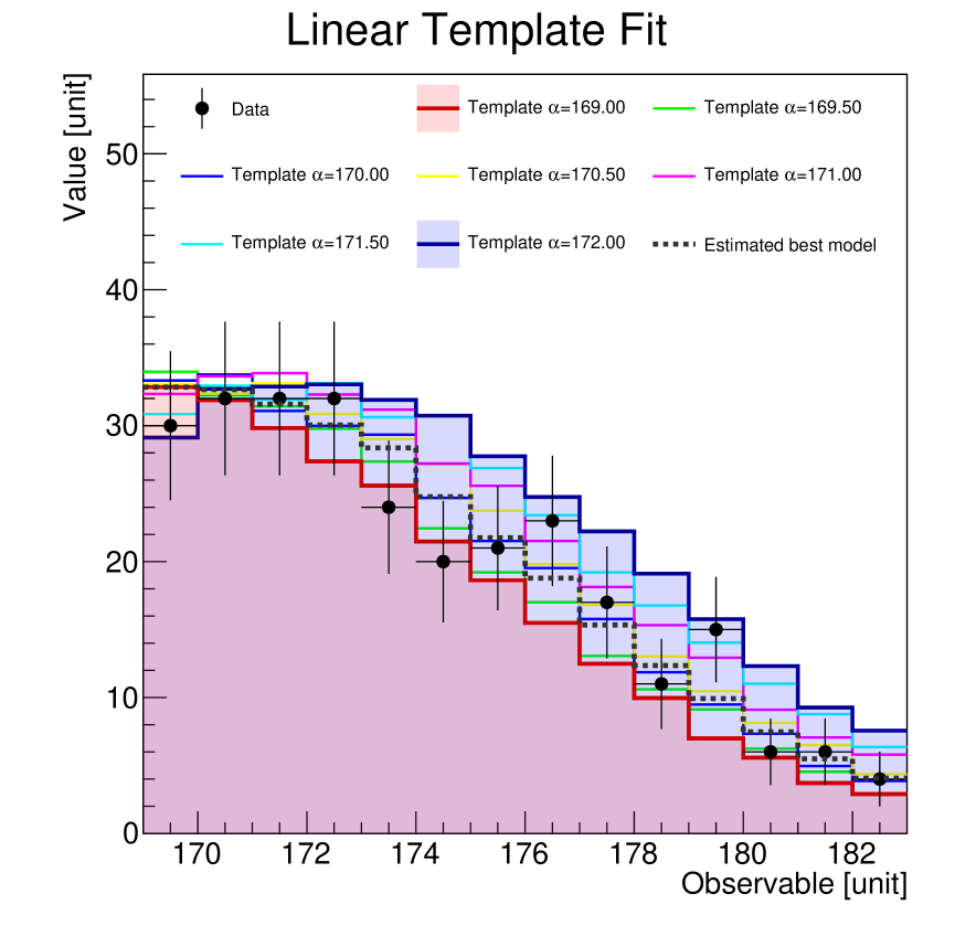
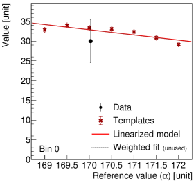
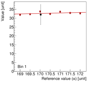
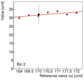
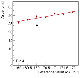
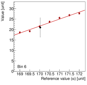
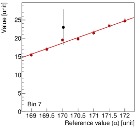
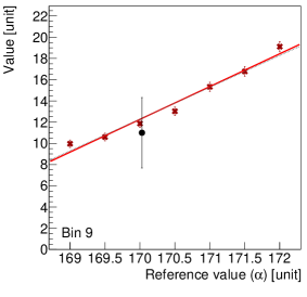
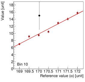
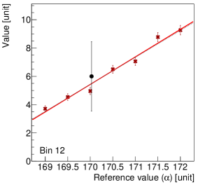
Figure 1: Two views of the template matrix $Y$ of an example application of the Linear Template Fit. Left: the template distributions $Y$ as a function of the observable. The full circles display a pseudo-data set with statistical uncertainties, and the dotted line indicates the estimated model after the fit, ${\mathbf{y}}(\hat{\alpha})$. Right: the template distributions $Y$ of an example application of the Linear Template Fit, but as a function of the reference values of the parameter of interest $\alpha$. Only nine selected ‘bins’ $i$ are displayed. The red line shows the linearized model $\hat{\mathrm{y}}_{i}(\alpha)$, eq. (15), in the respective bin, and the full circles are again the pseudo-data. The dotted line indicates a weighted linear regression, which is not used in the Linear Template Fit.

The Linear Template Fit using these seven templates is illustrated in figure 1. The Linear template Fit from eq. (19) reports a value of $\hat{\alpha}=170.03\pm 0.41$, which is fully consistent within the statistical uncertainty with the generated true value of 170.2, although a somewhat different standard deviation was used. In figure 1 (right), the result from a hypothesized weighted linear regression is shown (cf. eq. (23)), but it is almost indistinguishable from the unweighted linear regression as is used in the Linear Template Fit. This is because the generation of the individual templates always employs the same methodology, as already argued above. Furthermore, the estimated best model is displayed in figure 1 (left), which is defined from eq. (15) when substituting the best estimator, ${\hat{\mathbf{y}}}={\mathbf{y}}(\hat{\alpha})$. This results in $\chi^{2}=5.6$ for 14 data points and one free parameter. Other seeds for the random number generator of course result in different values. It should be noted that this example is purposefully constructed with large (statistical) uncertainties in order to obtain a visually clearer presentation in the figures, although in some bins the assumption of normal-distributed random variables is then a rather poor approximation to the Poisson distribution.

5 The multivariate Linear Template Fit

Phenomenological models often depend on multiple parameters, and thus it is a common task to determine multiple parameters at a time. Such $k$ parameters of interest are referred to as $\alpha_{1}$, …, $\alpha_{k}$, or simply $\bm{\alpha}$, and the best estimators are denoted as $\hat{\alpha}_{1}$, …, $\hat{\alpha}_{k}$, or $\bm{\hat{\alpha}}$. The linear representation of the model is a hyperplane $\rm{y}_{i}(\bm{\alpha})$ in each of the $i$ data points, defined as

$$\bm{\lambda}(\bm{\alpha})\approx\mathbf{y}(\bm{\alpha};{\bm{\hat{\theta}}})=\hat{\theta}_{0}+\hat{\theta}_{(1,1)}\alpha_{1}+\dots+\hat{\theta}_{(1,k)}\alpha_{k}\,,$$ (24)

where a constant $\theta_{0}$ and the first-degree parameters $\theta_{(1,k)}$ are considered. Since higher-degree terms or interference terms are not included, the fit parameters need to be (sufficiently) independent or they have been made orthogonal by applying a variable transformation beforehand.

In the multivariate case, each template $\bm{y}_{(j)}$ is representative of a reference point $\bm{\dot{\alpha}}_{(j)}$ in the $k$-dimensional space. The regressor matrix $M$ is constructed as a $j\times(1+k)$ design matrix:

$$M:=\left(\begin{matrix}1&\dot{\alpha}_{(1),1}&\dots&\dot{\alpha}_{(1),k}\\ \vdots&\vdots&\vdots&\vdots\\ 1&\dot{\alpha}_{(j),1}&\dots&\dot{\alpha}_{(j),k}\\ \end{matrix}\right)\,.$$ (25)

As in the univariate case, the pseudoinverse $M^{+}$ is calculated from eq. (12), and also the same considerations for the justification of the unweighted multiple regression are applicable. Instead of a single vector $\bm{\tilde{m}}$, there is now a vector for each regression parameter $\theta_{k}$. Therefore, the $j\times k$ matrix $\tilde{M}$ is introduced, which is defined by decomposing $M^{+}$ like

$$M^{+}=:\begin{pmatrix}\bm{\bar{m}}^{\text{T}}\\ \tilde{M}^{\text{T}}\\ \end{pmatrix}\,.$$ (26)

Hence, the best estimator for the linearized multivariate model $\mathbf{y}(\bm{\alpha};{\bm{\theta}})$ becomes

$$\bm{\lambda}(\bm{\alpha})\approx{\hat{\mathbf{y}}}(\bm{\alpha})=Y\bm{\bar{m}}+Y\tilde{M}\bm{\alpha}\,,$$ (27)

where the $\theta$-parameters are again no longer explicit.

When using the linear approximation of the model, $\bm{\lambda}(\bm{\alpha})\approx\hat{\mathbf{y}}(\bm{\alpha})$, the $\chi^{2}$ function (eq. (2)) for the multivariate Linear Template Fit becomes

$$\chi^{2} \simeq\left(\bm{d}-\hat{\mathbf{y}}(\bm{\alpha})\right)^{\text{T}}W\left(\bm{d}-\hat{\mathbf{y}}(\bm{\alpha})\right)$$ (28)

$$=\left(\bm{d}-Y\bm{\bar{m}}-Y\tilde{M}\bm{\alpha}\right)^{\text{T}}W\left(\bm{d}-Y\bm{\bar{m}}-Y\tilde{M}\bm{\alpha}\right)$$ (29)

$$=\left(\bm{d}-{\textstyle\sum}_{l}\hat{\epsilon}_{l}\bm{s}_{(l)}-\hat{\mathbf{y}}(\bm{\alpha})\right)^{\text{T}}\mathbb{V}^{-1}\left(\bm{d}-{\textstyle\sum}_{l}\hat{\epsilon}_{l}\bm{s}_{(l)}-\hat{\mathbf{y}}(\bm{\alpha})\right)+{\textstyle\sum}_{l}\hat{\epsilon}_{l}^{2}\,.$$ (30)

The last equation introduces an equivalent expression in terms of nuisance parameters [63]. The factors $\hat{\epsilon}_{l}$ are related to uncertainties with full bin-to-bin correlations when writing the covariance matrix as

$$V=\mathbb{V}+V_{\textrm{corr}}~{}~{}~{}\text{ using}~{}~{}~{}V_{\textrm{corr}}=\textstyle\sum_{l}\bm{s}_{(l)}\bm{s}^{\text{T}}_{(l)}\,,$$ (31)

where the sum $l$ runs over all uncertainties with full bin-to-bin correlations and the vectors $\bm{s}_{l}$ denote the individual systematic uncertainties (also called shifts), while the matrix $\mathbb{V}$ includes all other uncertainty components. It is common practice that the systematic shifts are calculated from relative uncertainties and multiplied with the measured data. Implications of this practice are discussed in section 7 and 8.7, and care must be taken that the result does not become biased [64, 65, 66, 67, 68, 69]; a common technique to avoid that bias is discussed in section 8.7.

Equation (30) is again a linear least squares expression and the best linear unbiased estimators for the parameters $\bm{\hat{\alpha}}$ and the nuisance parameters $\bm{\hat{\epsilon}}$ are obtained from the stationary point. Hence, the best estimators from the multivariate Linear Template Fit become

$$\bm{\hat{a}}=\begin{pmatrix}\bm{\hat{\alpha}}\\ \bm{\hat{\epsilon}}\end{pmatrix}=\mathcal{F}(\bm{d}-Y\bm{\bar{m}})\,,$$ (32)

where $\bm{\hat{a}}$ was introduced and the shorthand notations $\mathcal{F}$ (a $g$-inverse of least squares) and $\mathcal{D}$ are calculated as

$$\mathcal{F}:=\mathcal{D}^{-1}\begin{pmatrix}Y\tilde{M}&~{}S\end{pmatrix}^{\text{T}}\mathbb{W}:=\left(\begin{pmatrix}Y\tilde{M}&~{}S\end{pmatrix}^{\text{T}}\mathbb{W}\begin{pmatrix}Y\tilde{M}&~{}S\end{pmatrix}+\begin{pmatrix}{0}_{k}&0\\ 0&{1}_{l}\end{pmatrix}\right)^{-1}\begin{pmatrix}Y\tilde{M}&~{}S\end{pmatrix}^{\text{T}}\mathbb{W}\,,$$ (33)

using $\mathbb{W}=\mathbb{V}^{-1}$. The matrix with the fully bin-to-bin correlated uncertainties $S$ is composed from the column-vectors of the systematic shifts $\bm{s}_{(l)}$ as

$$S:=\begin{pmatrix}\bm{s}_{(1)}&\ldots&\bm{s}_{(l)}\end{pmatrix}\,,$$ (34)

and the symbol $\begin{pmatrix}Y\tilde{M}&~{}S\end{pmatrix}$ denotes a composed $i\times(k+l)$ matrix from $Y\tilde{M}$ and $S$, while ${0}_{k}$ and ${1}_{l}$ denote a $k\times k$ or $l\times l$ zero or unit-matrix, respectively. The matrix $\mathcal{D}$ is commonly a full-ranked symmetric matrix and thus invertible. A brief discussion about a more efficient numerical calculation of $\mathcal{D}^{-1}$ is given in D. If all uncertainty components are represented through a single covariance matrix $V$, cf. left side of eq. (31), the multivariate Linear Template Fit simplifies to

$$\bm{\hat{\alpha}}=\left((Y\tilde{M})^{\text{T}}WY\tilde{M}\right)^{-1}(Y\tilde{M})^{\text{T}}W(\bm{d}-Y\bm{\bar{m}})\,.$$ (35)

6 Example 2: the multivariate Linear Template Fit

In Example 1, only the mean value of the model (which is a normal-distribution) was determined, although the pseudo-data had a slightly different standard deviation than the model. In the following example, a multivariate Linear Template Fit is performed and the same pseudo-data as in Example 1 are used, but both values of the model will be determined: the mean value and the standard deviation of the Gaussian. Therefore, templates are generated for some selected values for the mean (between values of 169.5 and 171) and the standard deviation (between values of 5.8 and 6.4) of a Gaussian, and again 40,000 events are used for each template. The four “extreme” variations of the two parameters are omitted. The multivariate Linear Template Fit using all these templates is illustrated in figure 2.

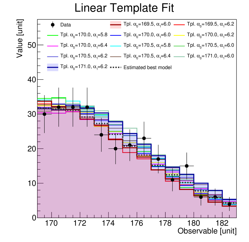
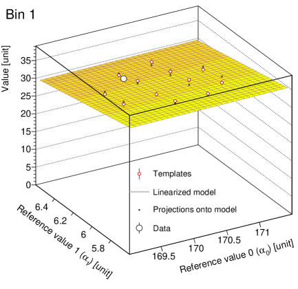
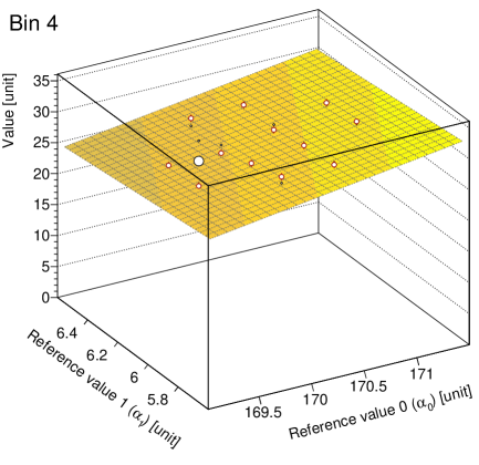
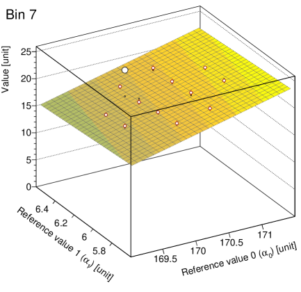
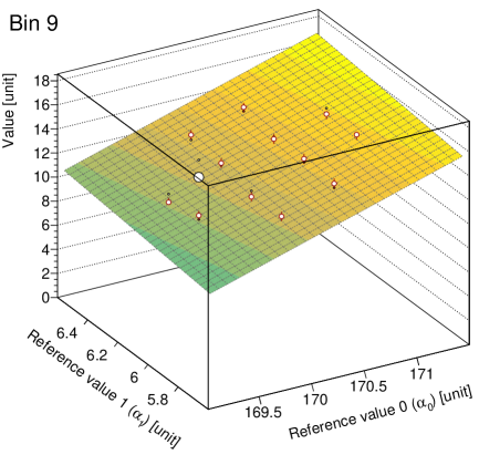
Figure 2: Two views of the template matrix $Y$ of an example application of the multivariate Linear Template Fit. Left: the template distributions $Y$ as a function the observable. More details are given in the caption of figure 1. Right: the template distributions $Y$ (open medium-sized circles) as a function of the two reference values for four selected “bins” $i$. The plane displays the linearized model $\hat{\mathrm{y}}_{i}(\bm{\alpha})$, eq. (27), in the respective bin. The large open circles are again the pseudo-data, and small circles indicate the projection onto the plane $\hat{\mathrm{y}}$.

The best estimators from the multivariate Linear Template Fit (eq. (35)) are $169.91\pm 0.46$ for the mean and $6.28\pm 0.38$ for the standard deviation. Their correlation coefficient is found to be $-0.3$. Within the statistical uncertainties, both values are in very good agreement with the simulated input values of $170.2$ and $6.2$, respectively. Thus, this example illustrates the application of the multivariate Linear Template Fit with two free parameters, where a visual representation of the linearized model is still possible. However, any number of free parameters is in principle possible, and for an $n$-parameter fit, the minimum number of linearly independent templates is just $n+1$.

7 The Linear Template Fit with relative uncertainties

In this section we present the equations for the Linear Template Fit when the estimators obey a log-normal distribution. This could be the case for data when the determination of a variable is affected by a number of multiplicative factors that are subject to uncertainties. Consequently, the variable follows a log-normal distribution due to the central limit theorem [48, 49]. Also, when the value of an observed variable is a random proportion of the previous observation, it follows a log-normal distribution [49]. An example would be the measurement of the electron energy in a calorimeter which is affected by a number of fractional energy losses and corrections [10]. Another example would be measurements that are dominated by systematic multiplicative uncertainties: a prominent multiplicative error is due to uncertainties of the luminosity measurement in particle collider experiments which results in a relative uncertainty. Contrary to additive errors, multiplicative errors cannot change the sign of the variable, and a positively defined observable always remains positive, which is an important prerequisite for several physical quantities such as cross sections. A comparison of the log-normal, the normal, and the Poisson probability distribution function for two selected values of their mean value are displayed in figure 3.

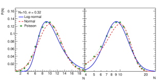
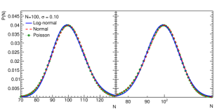
Figure 3: The log-normal, normal, and Poisson probability distribution functions with mean values of 10 (left) and 100 (right) on a linear and logarithmic axis. These values are commonly referred to as relative uncertainties of 32 % and 10 %, respectively. For larger uncertainties, the log-normal distribution provides a good approximation of the Poisson distribution around the peak. The log-normal and the Poisson distributions are strictly positive. For large $N$, all distributions become similar.

The likelihood of a set of $i$ measurements is a joint function of log-normal probability distribution functions

$$\mathcal{L}=\prod_{i}^{N}\frac{1}{\sqrt{2\pi\varsigma_{i}^{2}d_{i}^{2}}}\exp\left(\frac{-(\log{d_{i}}-\mu_{i})^{2}}{2\varsigma_{i}^{2}}\right)\,.$$ (36)

When writing $\mu_{i}=\log m_{i}$ [70, 71], it can be directly seen from the residuals that the ratios $d_{i}/m_{i}$ enter the likelihood calculation instead of their differences. The variance $\varsigma$ denotes a relative quantity, thus it represents relative uncertainties. In fact, the log-normal distribution is equivalent to considering random variables with normal-distributed relative uncertainties. For small relative errors, $\varsigma_{i}\lesssim 20\,\%$, which is a common case in particle physics, the log-normal, the normal, and the Poisson distributions become similar. For larger relative errors, the log-normal distribution provides some approximation of the Poisson distribution, and for practical purposes one benefits from its strictly positiveness, in contrast to the often used normal distribution.

Similarly to the case for normal-distributed data, we choose as a first-order approximation of the model in every bin

$$\mu_{i}(\bm{\alpha})\approx\theta^{(i)}_{0}+\theta^{(i)}_{(1,1)}\alpha_{1}+\ldots+\theta^{(i)}_{(1,k)}\alpha_{k}\,,$$ (37)

and the best estimators for the $\theta$ parameters are again determined from the templates; consequently, the best estimator of the approximated model is

$$\bm{\mu}(\bm{\alpha})\approx\bm{\hat{{\mu}}}(\bm{\alpha})=\log(Y)\bm{\bar{m}}+\log(Y)\tilde{M}\bm{\alpha}\,.$$ (38)

The term $\log(Y)$ denotes a coefficient-wise application of the logarithm to the elements of the template matrix $Y$, and it is used to match the logarithmized data ($\log{d_{i}}$) in the likelihood. Eq. (38) is an equally valid first-order approximation of the model as compared with the default linear approximation in eq. (24).

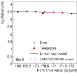
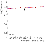
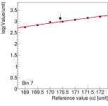
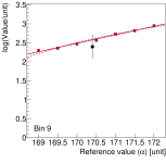
Figure 4: The best estimate of the parameter dependence of the model, eq. (38) for four selected bins of Example 1, when performing a Linear Template Fit with log-normal distributed estimators. Note that the $y$ axis indicates the logarithmized values of the templates. The pseudo-data are displayed for comparison at the best estimator $\hat{\alpha}$ of the Linear Template Fit. For comparison, the linearized model from eq. (15) is also displayed, which is otherwise not used when log-normal-distributed estimators are considered.

As an illustration, the linearized model from eq. (38) is displayed in figure 4 for some selected bins of Example 1 (section 4) and compared with the approximations of eq. (27). The two are reasonably similar in that example, since the templates are present in the vicinity of the best estimator and in a range where a linear approximation is valid. Although the parameter dependence in Example 1 is in fact truly linear, from the generated statistical precision of the templates, the templates cannot discriminate between these two best model estimators.

When using log-normal distributed variables, which corresponds to relative uncertainties, the objective function $\chi^{2}$  of the Linear Template Fit becomes

$$\chi^{2}=\left(\bm{\log d}-{\textstyle\sum}_{l}\epsilon_{l}\mathbf{s}_{(l)}-\bm{\hat{\mu}}(\bm{\alpha})\right)^{\text{T}}\mathbb{W}\left(\bm{\log d}-{\textstyle\sum}_{l}\epsilon_{l}\mathbf{s}_{(l)}-\bm{\hat{\mu}}(\bm{\alpha})\right)+{\textstyle\sum}_{l}\epsilon_{l}^{2}\,.$$ (39)

The covariance matrix $\mathbb{V}=\mathbb{W}^{-1}$ comprises normal-distributed relative uncertainties, and also the uncertainties with bin-correlations $\mathbf{s}$ enter the calculation through their relative values. The notation $\bm{\log d}$ denotes a coefficient-wise application of the logarithm. A common relation between relative and absolute uncertainties would be

$$\mathrm{s}_{(l),i}\simeq\frac{s_{(l),i}}{d_{i}}\,,$$ (40)

and although this equation does not strictly translate between normal and log-normal uncertainties, it is often used in practical applications. Note that we use a Roman font s for relative uncertainties, and italic $s$ for absolute uncertainties.

This $\chi^{2}$ function is again a linear least-squares problem, and the best estimators for $\bm{\alpha}$ and $\bm{\epsilon}$ in the Linear Template Fit are

$$\bm{\hat{a}}:=\left(\begin{matrix}\bm{\hat{\alpha}}\\ \bm{\hat{\epsilon}}\\ \end{matrix}\right)=\mathcal{F}\big{(}\bm{\log d}-\log(Y)\bm{\bar{m}}\big{)}\,,$$ (41)

where the matrix $\mathcal{F}$ is defined in a similar way as eq. (33), but from relative uncertainties in $\mathbb{V}$ and $\mathrm{s}$ ($S$) and employing the substitution $Y\tilde{M}\to\log(Y)\tilde{M}$. Due to the treatment of systematic uncertainties as relative uncertainties, the Linear Template Fit with the log-normal probability distribution functions may be preferred in practical applications over the Linear Template Fit with absolute uncertainties.

When repeating Example 1 (section 4) with relative uncertainties, the best estimator for the mean value is found according to eq. (41) to be $\hat{\alpha}=170.40\pm 0.46$, which is in good agreement to the generated value of 170.2. Some details are further displayed in figure 4. When considering Example 2 (section 6) under the assumption of log-normal distributed pseudo-data, the best estimators are found to be $170.18\pm 0.47$ for the mean and $6.33\pm 0.39$ for the standard deviation, with a correlation coefficient of $-0.3$. When considering further a normalisation uncertainty of the size of 10 %, so a relative uncertainty, the best estimators for the mean and variance become $\alpha_{0}=170.20\pm 0.76$ and $\alpha_{1}=6.33\pm 0.49$, respectively. Their correlation coefficient is $-0.6$, and the nuisance parameter of the normalisation uncertainty is $\hat{\epsilon}=-0.02\pm 0.5$.

8 Errors and error propagation

In many applications and fields, like particle physics, it is of great importance to provide detailed uncertainties together with the fit parameters and to propagate uncertainties from all relevant input quantities. Due to its analytic and closed form, the Linear Template Fit provides unique opportunities for detailed error propagation and analysis, that is otherwise not easily possible in other inference algorithms. For example, every single uncertainty component can be propagated separately and analytically to the fit results. In the following, the equations for error propagation are discussed, based on the equation of the Linear Template Fit in eq. (32).

8.1 Statistical uncertainties and uncertainties without bin-to-bin correlations

Statistical or epistemic uncertainties in the data are represented by the covariance matrix $\mathbb{V}$. The matrix $\mathbb{V}$ may include further uncertainty components with or without bin-to-bin correlations, like systematic or aleatoric uncertainties. From linear error propagation [60], the covariance matrix is propagated to the best estimators $\bm{\hat{a}}$ as

$$\hat{\mathbb{V}}_{\bm{\hat{a}}}=\mathcal{F}\mathbb{V}\mathcal{F}^{\text{T}}\,,$$ (42)

using $\mathcal{F}$ as defined in eq. (33). Due to the Gauß–Markov theorem the estimators $\bm{\hat{a}}$ for the given objective function $\chi^{2}$, eqs. (30) and (39), have the least variance among all possible estimators.

If $\mathbb{V}$ is a sum of multiple individual matrices, like $\mathbb{V}=\mathbb{V}_{\textrm{stat.}}+\sum\mathbb{V}_{\textrm{uncorr.}}+\sum\mathbb{V}_{\textrm{corr.}}+\ldots$, each covariance matrix can be propagated separately using equation (42). By doing so, the contribution from each uncertainty component to the full uncertainty is determined separately.

8.2 Systematic uncertainties or uncertainties with bin-to-bin correlations

Systematic uncertainties associated with the input data are often represented as uncertainties with full bin-to-bin correlations and are represented either as systematic shifts, $\bm{s}_{(l)}$ (eq. (34)), or as covariance matrices, $\mathbb{V}_{l}^{\textrm{corr}}=\bm{s}_{(l)}\bm{s}_{(l)}^{\text{T}}$. Using linear error propagation, these are propagated to the best estimators $\bm{\bm{\hat{a}}}$ as

$$\bm{\sigma}_{\bm{\hat{a}}}^{(\bm{s}_{(l)})}=\mathcal{F}\bm{s}_{(l)}\,.$$ (43)

Alternatively, eq. (42) can be employed. For the Linear Template Fit with relative uncertainties, one literally has the same equation but using relative values $\mathbf{s}_{(l)}$ (compare eq. (40)).

In Example 2, where a normalisation uncertainty of 10 % was considered the uncertainty breakdown for the two parameters would be $\sigma_{\hat{\alpha}_{0}}=\pm 0.56_{\text{(stat.)}}\pm 0.51_{\text{(norm.)}}$ and $\sigma_{\hat{\alpha}_{1}}=\pm 0.42_{\text{(stat.)}}\pm-0.25_{\text{(norm.)}}$.

When systematic uncertainties are included in the Linear Template Fit, their corresponding nuisance parameters $\epsilon_{l}$ are constrained by data, and the obtained reduction of the systematic uncertainty may be used for further analyses. In applications where the fitted parameters are dominated by systematic uncertainties in the input data, it is good practice to constrain the associated systematic shifts by adding additional measurements to the fitting problem [31, 72, 35, 73]. This practice provides additional constraints on the related parameters, $\epsilon_{l}$, and smaller experimental uncertainties can be obtained. The uncertainty in the nuisance parameter becomes smaller than unity.

8.3 External uncertainties

The generalized transfer matrix $\mathcal{F}$ provides the straightforward opportunity for linear error propagation; see eqs. (42) or (43). While these equations are predominantly employed to propagate the uncertainties that are included in the Linear Template Fit, equivalent equations are also applicable to propagate further uncertainties that are not used in the fit, but which would still need to be propagated to the fit result. For example, these may be uncertainties in the underlying theory prediction which cannot be constrained by the data. An actual case for such an uncertainty is given below for the non-perturbative correction factors (cf. Fig. 10).

8.4 Unconstrained uncertainties with full bin-to-bin correlations

A special case of an uncertainty with full bin-to-bin correlations may be considered through an unconstrained systematic uncertainty. These are defined by including the respective systematic shift $s_{(l)}$ into the Linear Template Fit, but in contrast to common constrained systematic uncertainties, these have a zero value (instead of unity) in the respective diagonal element of the $l\times l$ matrix ${1}_{l}$ in eq. (33). As a consequence, the Linear Template Fit can exploit the degree of freedom of that systematic shift, but the data does not provide any constraint on that uncertainty source. A possible application would be fits to data, where the normalization is unknown and is a free, unconstrained, systematic uncertainty.

8.5 Uncertainties in the templates

The template distributions $Y$ may be associated with uncertainties from various sources. These can be statistical uncertainties in the elements $Y_{ij}$ or systematic uncertainties with correlations among all entries of $Y$. One may think about $Y$ being determined from two distinct models, or templates that were generated with different parameters, and the resulting difference in $Y$ may be considered as a systematic uncertainty.

The uncertainties in $\bm{\hat{a}}$ due to uncertainties in $Y$ are obtained from linear error propagation. The uncertainty in a single element of $Y$ is denoted as $\sigma_{Y_{ij}}$, and using the shorthand notation $\mathcal{D}$ from eq. (33), the partial derivative of eq. (32) is

$$\frac{\partial\bm{\hat{a}}}{\partial Y_{ij}}=\mathcal{D}^{-1}\Bigg{[} \begin{pmatrix}\mathbb{1}_{(ij)}\tilde{M}&{0}_{il}\end{pmatrix}^{\text{T}}\mathbb{W}(\bm{d}-Y\bm{\bar{m}})-\begin{pmatrix}Y\tilde{M}&S\end{pmatrix}^{\text{T}}\mathbb{W}\mathbb{1}_{(ij)}\bm{\bar{m}}$$

$$-\left[\begin{pmatrix}Y\tilde{M}&S\end{pmatrix}^{\text{T}}\mathbb{W}\begin{pmatrix}\mathbb{1}_{(ij)}\tilde{M}&{0}_{il}\end{pmatrix}+\begin{pmatrix}\mathbb{1}_{(ij)}\tilde{M}&{0}_{il}\end{pmatrix}^{\text{T}}\mathbb{W}\begin{pmatrix}Y\tilde{M}&S\end{pmatrix}\right]\bm{\hat{a}}\Bigg{]}\,,$$ (44)

where $\mathbb{1}_{(ij)}$ denotes an $i\times j$ zero matrix with only the element $(i,j)$ being unity, and ${0}_{il}$ denotes an $i\times l$ zero-matrix. It should be noted, that the usage of the matrices $\mathbb{1}_{(ij)}$ and ${0}_{il}$ in numerical calculations is discouraged since a naive matrix multiplication becomes numerically inefficient, but that it remains instructive to write the equations in that extensive format. The resulting size of the uncertainty of the best estimators due to $\sigma_{Y_{ij}}$ becomes

$$\bm{\sigma}^{(Y_{ij})}_{\bm{\hat{a}}}=\frac{\partial\bm{\hat{a}}}{\partial Y_{ij}}\sigma_{Y_{ij}}\,.$$ (45)

Hence, uncertainties without entry-to-entry correlations, such as statistical uncertainties, are propagated to the estimated parameters as

$$\bm{\sigma}^{(Y_{\text{uncorr.}})}_{\bm{\hat{a}}}=\sqrt{\sum_{i,j}\bigg{(}\frac{\partial\bm{\hat{a}}}{\partial Y_{ij}}\sigma_{Y_{ij}}\bigg{)}^{2}}\,,$$ (46)

where the square root and the exponentiation are performed coefficient-wise, while uncertainties that have full entry-to-entry correlations are propagated as

$$\bm{\sigma}^{(Y_{\text{corr.}})}_{\bm{\hat{a}}}=\sum_{i,j}\frac{\partial\bm{\hat{a}}}{\partial Y_{ij}}\sigma_{Y_{ij}}\,.$$ (47)

In Example 1 and 2 (sections 4 and 6), the templates are each generated with 40 000 events and independently from each other. Hence, all their entries have statistical uncertainties. Using eq. (46), the statistical uncertainties from $Y$ under gaussian approximation are $\pm 0.025$ in Example 1, and $\pm 0.042$ and $\pm 0.060$ for the two parameters in Example 2.

The equations for error propagation of the Linear Template Fit with relative uncertainties (section 7) are altogether similar to the presented equations and do not need to be repeated. However, since relative uncertainties are considered, the partial derivatives for error propagation in eqs. (46) and (47) become

$$\frac{\tiny\partial\bm{\hat{a}}}{\partial Y_{tj}}\to\frac{\tiny\partial\bm{\hat{a}}}{\partial\log{Y_{tj}}}\,.$$ (48)

Example 2 with log-normal uncertainties would report statistical uncertainties from $Y$ of $\pm 0.052$ and $\pm 0.066$ for the two fit parameters.

Note that the uncertainties in $Y$ are not considered within the fit, but propagated separately, since it is assumed that these are negligibly small, and independent of the model parameter $\bm{\alpha}$, and cannot be constrained by the data.

8.6 Full uncertainty

The covariance matrix for the best estimators, including all uncertainty components that are considered in the Linear Template Fit, are calculated from eqs. (42) and (43):

$$V_{\bm{\hat{a}}}=\mathbb{V}_{\bm{\hat{a}}}+{\textstyle\sum}_{l}\bm{\sigma}_{\bm{\hat{a}}}^{(\bm{s}_{(l)})}(\bm{\sigma}_{\bm{\hat{a}}}^{(\bm{s}_{(l)})})^{\text{T}}$$ (49)

Further uncertainties, which are not explicitly considered in the fit, can be propagated to the result by using eqs. (42) and (43) or also eqs. (46) and (47).

8.7 Error (re-)scaling

When multiple data points are considered in the fit and they are correlated through some (systematic) uncertainties, the best-fit estimators may become biased [64, 65, 66, 67, 68, 69]. This is mainly because uncertainties with bin-to-bin correlations are commonly valid as relative uncertainties, or so-called multiplicative uncertainties, such as normalization uncertainties, but those are included in the fit with absolute values (i.e., as variances). Since the data are subject to random noise from statistical fluctuations, or simply because of the different size of the values, for example when considering different data sets, the result may become biased since smaller values are effectively preferred by the fit. While such a bias is largely reduced or even absent from first principles when working with relative uncertainties, it may still be useful to discuss possible solutions to this problem and several solutions are discussed in the literature (see e.g. Ref. [69]).

A common solution is to consider (multiplicative) uncertainties with bin-to-bin correlations through their relative values in the $\chi^{2}$ computation, and their relative values are multiplied coefficient-wise with the prediction(s) rather than the data values [68]. However, since the minimization of $\chi^{2}$ is then no longer linear in the fit parameters, there is no closed analytic solution for the best estimators. However, an approximately equivalent result is obtained when calculating the covariance matrices and systematic shifts (cf. eq. (31)) from theoretical predictions [66], and the coefficients of the shifts are recalculated according to

$$s_{(l),i}\to\frac{s_{(l),i}y_{i}}{d_{i}}\,=\mathrm{s}_{(l),i}y_{i},$$ (50)

and analogously for covariance matrices. Various options for the predictions $\bm{y}$ for this error rescaling may be considered, and the prediction $\bm{y}$ could be chosen to be

• One of the template distributions, $\bm{y}_{(j)}$;

• The prediction of the linearized model with ad-hoc selected parameters $\bm{\alpha}$, $\mathbf{\hat{y}}(\bm{\alpha})$;

• The best estimator of the linear model, $\mathbf{\hat{y}}(\bm{\hat{a}})$; or

• The Linear Template Fit may be iteratively repeated with the best estimator, $\mathbf{\hat{y}}(\bm{\hat{a}})$.

The rather compact equations of the Linear Template Fit are well suited for an iterative algorithm. Such procedures are equivalent to an alternative formulation of the $\chi^{2}$ quantity, but the convergence of such iterative algorithms should be critically assessed.

9 Linear Template Fit with a detector response matrix

Many measurements need to be corrected for detector effects like resolution or acceptance in order to compare the measurement with theoretical predictions. This is referred to as unfolding (for reviews see e.g. [74, 10, 75, 76, 77, 78, 79]) and is commonly performed by first simulating the detector response and representing it in terms of a response matrix $A$,

$$\bm{y}=A\bm{x}\,,$$ (51)

where $\bm{y}$ denotes the measured detector-level distribution and $\bm{x}$ the “true” underlying distribution. However, it is not straightforward to apply the inverse response matrix to the distribution $\bm{y}$, since the unfolding problem represents an ill-posed inverse problem, or the matrix $A$ needs to be a square matrix, and thus more sophisticated unfolding algorithms need to be employed to determine the “true” distribution $\bm{x}$ [80, 81, 82, 83, 84, 85]. When performing a parameter determination, however, it is equivalent whether using the unfolded distribution $x$ together with templates of the predictions, or alternatively using the detector-level measurement $y$ and applying the response matrix to the templates instead. These two procedures are supposed to be equivalent if the unfolding problem and algorithm are unbiased, and are referred to as folding, up-folding, or forward folding. Because the simulation of the detector effects and the determination of the response matrix $A$ may be computationally expensive, as is the case for complex particle physics experiments, it may be reasonable to determine the matrix $A$ only once and with high precision, and then apply it to the templates.

The inclusion of the detector effects in the Linear Template Fit is straightforward and is realized by the simple substitution

$$Y \rightarrow AX$$ (52)

in eqs. (32) and (33), where $X$ represents the template matrix without detector effects at the “truth” or “particle” level. When using relative uncertainties, the substitution becomes

$$\log(Y)\to\log(AX)\,,$$ (53)

and the full expression of the Linear Template Fit becomes

$$\small\begin{pmatrix}\bm{\hat{\alpha}}\\ \bm{\hat{\epsilon}}\end{pmatrix}=\mathcal{F}\big{(}\bm{\log d}-\log(AX)\bm{\bar{m}}\big{)}~{}~{}~{}\text{using}\\$$

$$\mathcal{F}=\left(\begin{pmatrix}\log(AX)\tilde{M}&~{}S\end{pmatrix}^{\text{T}}\mathbb{W}\begin{pmatrix}\log(AX)\tilde{M}&~{}S\end{pmatrix}+\begin{pmatrix}{0}_{k}&0\\ 0&{1}_{l}\end{pmatrix}\right)^{-1}\begin{pmatrix}\log(AX)\tilde{M}&~{}S\end{pmatrix}^{\text{T}}\mathbb{W}\,.$$ (54)

Since $Y$ and $AX$ are $i\times j$ matrices, the index $t$ for the number of entries (“bins”) on the truth level was introduced. Thus, $A$ is an $i\times t$ matrix and $X$ has dimension $t\times j$, and in order to obtain a higher resolution, it may be reasonable to consider a non-square response matrix $A$, i.e., $i\neq t$. It is important that the detector response $A$ is required to be independent from the physics parameter of interest.

The response matrix $A$ is typically associated with uncertainties, and these may be entry-to-entry correlations (like systematic or “model” uncertainties) or without such correlations (like statistical uncertainties). Note, that the response matrix is commonly normalized and therefore the statistical uncertainties are without entry-to-entry correlations only approximately.

Uncertainties of the best estimators that arise from uncertainties in $A$ can be obtained from linear error propagation. After applying eq. (52), the partial derivative of eq. (32) is

$$\frac{\partial\bm{\hat{a}}}{\partial A_{it}}=\mathcal{D}^{-1}\Bigg{[} \begin{pmatrix}\mathbb{1}_{(it)}X\tilde{M}&{0}_{il}\end{pmatrix}^{\text{T}}\mathbb{W}(\bm{d}-AX\bm{\bar{m}})-\begin{pmatrix}AX\tilde{M}&S\end{pmatrix}^{\text{T}}\mathbb{W}\mathbb{1}_{(it)}X\bm{\bar{m}}$$

$$-\left[\begin{pmatrix}AX\tilde{M}&S\end{pmatrix}^{\text{T}}\mathbb{W}\begin{pmatrix}\mathbb{1}_{(it)}X\tilde{M}&{0}_{il}\end{pmatrix}+\begin{pmatrix}\mathbb{1}_{(it)}X\tilde{M}&{0}_{il}\end{pmatrix}^{\text{T}}\mathbb{W}\begin{pmatrix}AX\tilde{M}&S\end{pmatrix}\right]\bm{\hat{a}}\Bigg{]}\,,$$ (55)

Consequently, uncertainties in the response matrix $A$ without or with entry-to-entry correlations are propagated to the fitted results as

$$\bm{\sigma}^{(A_{\text{uncorr.}})}_{\bm{\hat{a}}}=\sqrt{\sum_{i,t}\left(\frac{\partial\bm{\hat{a}}}{\partial A_{it}}\sigma_{A_{it}}\right)^{2}}~{}~{}~{}\text{and}~{}~{}~{}\bm{\sigma}^{(A_{\text{corr.}})}_{\bm{\hat{a}}}=\sum_{i,t}\frac{\partial\bm{\hat{a}}}{\partial A_{it}}\sigma_{A_{it}}\,,$$ (56)

respectively, where $\sigma_{A_{it}}$ denotes the size of the uncertainty in the element $A_{it}$, and the power and square-root operations are applied coefficient-wise. When using a response matrix, the uncertainties in the template matrix $X$ (cf. section 8.5) are propagated using

$$\frac{\tiny\partial\bm{\hat{a}}}{\partial X_{tj}}=\mathcal{D}^{-1}\Bigg{[} \begin{pmatrix}A\mathbb{1}_{(tj)}\tilde{M}&{0}_{il}\end{pmatrix}^{\text{T}}\mathbb{W}\left(\bm{d}-AX\bm{\bar{m}}\right)-\begin{pmatrix}AX\tilde{M}&S\end{pmatrix}^{\text{T}}\mathbb{W}A\mathbb{1}_{(tj)}\bm{\bar{m}}$$

$$-\left[\begin{pmatrix}AX\tilde{M}&S\end{pmatrix}^{\text{T}}\mathbb{W}\begin{pmatrix}A\mathbb{1}_{(tj)}\tilde{M}&{0}_{il}\end{pmatrix}+\begin{pmatrix}A\mathbb{1}_{(tj)}\tilde{M}&{0}_{il}\end{pmatrix}^{\text{T}}\mathbb{W}\begin{pmatrix}AX\tilde{M}&S\end{pmatrix}\right]\bm{\hat{a}}\Bigg{]}\,.$$ (57)

Note that for the Linear Template Fit with relative uncertainties, it is reasonable to consider uncertainties in $A_{it}$ as absolute uncertainties, rather than relative, because the elements $A_{it}$ represent already relative quantities and may be interpreted as probabilities. Therefore, one employs the partial derivative $\partial\bm{\hat{a}}/\partial A_{ij}$ for error propagation, instead of $\partial\bm{\hat{a}}/\partial\log{A_{ij}}$, although elsewhere relative uncertainties are considered. This partial derivative is straightforward to derive. The propagation of uncertainties in the templates $X_{tj}$, however, becomes somewhat more complicated when using a response matrix $A$, since one has to calculate the partial derivative $\partial\bm{\hat{a}}/\partial\log{X_{tj}}$ for error propagation of the relative uncertainties $\sigma_{X_{tj}}$.

10 Considerations, validations and cross checks

As in any optimization problem, the result of the Linear Template Fit needs to be validated and cross checked. Due to its close similarity to the iterative Gauß–Newton minimization algorithm of nonlinear least squares [51, 5, 86, 87, 50], the Linear Template Fit is expected to result in an unbiased and optimal result, in particular if the templates provide a sufficiently accurate approximation of the model and its Jacobi matrix at the best estimator. In fact, when assuming that the model $\bm{\lambda}(\bm{\alpha})$ could be used with continuous values of $\bm{\alpha}$ for inference, the best estimator from the Linear Template Fit becomes equivalent to the best estimator that would be obtained when using $\bm{\lambda}(\bm{\alpha})$ directly, if two approximations are exactly fulfilled,

$$\bm{\lambda}(\bm{\hat{\alpha}}) \approx\mathbf{\hat{y}}(\bm{\hat{\alpha}})=Y\mathbf{\bar{m}}+Y\tilde{M}\bm{\hat{\alpha}}~{}~{}~{}~{}~{}\text{and}~{}$$ (58)

$$\left.\tfrac{\partial\bm{\lambda}(\bm{\alpha})}{\partial\bm{\alpha}}\right|_{\bm{\alpha}=\bm{\hat{\alpha}}} \approx\left.\tfrac{\partial\mathbf{\hat{y}}(\bm{\alpha})}{\partial\bm{\alpha}}\right|_{\bm{\alpha}=\bm{\hat{\alpha}}}=Y\tilde{M}\,.$$ (59)

The first equation requires that the model is correctly represented by the interpolated templates at the best estimator, which is needed for the value of the best estimator, and the second equation demands that the first derivatives are correctly approximated, which is a requirement for the error propagation and minimization. These equations taken together represent just a linear approximation of $\bm{\lambda}(\bm{\alpha})$ at $\bm{\hat{\alpha}}$, but using the templates only. However, since for the motivation of the Linear Template Fit it was assumed that $\bm{\lambda}(\bm{\alpha})$ cannot be used for inference itself, these two approximations also cannot be validated directly. In the following, some possible studies for the validation of the results and the practical application of the Linear Template Fit are discussed.

10.1 Template range

If the model is nonlinear in the parameters $\bm{\alpha}$, an unbiased result may only be obtained if the best estimator $\bm{\hat{\alpha}}$ lies within the interval of the reference values,

$$\bm{\hat{\alpha}}\in[\bm{\dot{\alpha}}_{(1)},\bm{\dot{\alpha}}_{(j_{\text{max}})}]\,.$$ (60)

This is because the templates provide the approximation of the model and its first derivatives, but an extrapolation beyond the template range is inappropriate for a non-linear model. If eq. (60) does not hold, additional templates at further reference points should be generated and the Linear Template Fit should be repeated with an improved selection of reference values. For similar reasons, the templates should be in the close vicinity of the best estimator, such that the linear approximations are justified. As a rule of thumb, the distance between the reference points should not greatly exceed the size of the variance of the best estimator

$$\bm{\dot{\alpha}}_{(j)}-\bm{\dot{\alpha}}_{(j+1)}\lesssim\bm{\sigma}_{\bm{\hat{\alpha}}}\,.$$ (61)

For similar reasons, the best-estimator should ideally be found in the center of the template range, rather than at its boundary,

$$\bm{\bm{\hat{a}}}-\bm{\dot{\alpha}}_{(0)}\approx\bm{\dot{\alpha}}_{(j_{\text{max}})}-\bm{\bm{\hat{a}}}\,.$$ (62)

However, for rather linear parameter dependencies these requirements may be more relaxed.

The choice of the reference values may be related to the size of the uncertainties of the best estimator. If one considers the uncertainties of the best estimator to be normal distributed, as a consequence, the model also needs to exhibit a sufficiently linear behavior at least within a few $\sigma$. As a rule of thumb, one could demand that the reference values are approximately within $3$ standard deviations:

$$\bm{\dot{\alpha}}_{(j)}\in[\bm{\hat{\alpha}}-3\bm{\sigma}_{\bm{\hat{\alpha}}},\bm{\hat{\alpha}}+3\bm{\sigma}_{\bm{\hat{\alpha}}}]\,.$$ (63)

10.2 The value of $\hat{\chi}^{2}$, its uncertainty and the partial $\chi^{2}$

The value of $\chi^{2}$ at the minimum, $\hat{\chi}^{2}$, is a meaningful quantity to assess the agreement between the data and the model. Since the calculation of $\chi^{2}$ is not explicit in the Linear Template Fit, its value needs to be calculated separately, and $\hat{\chi}^{2}$ is calculated from data and the templates at $\bm{\hat{a}}$ using the somewhat simplified equation

$$\hat{\chi}^{2}=\left(\bm{d}-Y\bm{\bar{m}}-Y\tilde{M}\bm{\hat{a}}\right)^{\text{T}}W\left(\bm{d}-Y\bm{\bar{m}}\right)\,.$$ (64)

Since the data and the templates are associated with uncertainties, the value of $\hat{\chi}^{2}$ consequently may also be considered as uncertain. The uncertainty in $\hat{\chi}^{2}$ is obtained from linear error propagation of the input uncertainties and calculated as

$$\sigma_{\hat{\chi}^{2}}=\sqrt{\bm{\xi}^{\text{T}}\mathbb{V}\bm{\xi}+\sum_{l}(\bm{\xi}\bm{s}_{(l)}^{\text{T}})^{2}}\,,$$ (65)

where the $i$-vector $\bm{\xi}$ is introduced and whose coefficients represent the partial derivatives $\tfrac{\partial\hat{\chi}^{2}}{\partial d_{i}}$, which are calculated as $\xi_{i}=2W_{i}(\bm{d}-\mathbf{\hat{y}}(\bm{\hat{a}}))$, and $W_{i}$ denotes the $i$th row of the matrix $W$. Also, the uncertainties in the templates $Y$ may be propagated to $\hat{\chi}^{2}$ with similar equations. The interpretation of $\sigma_{\hat{\chi}^{2}}$ is not trivial, but it may well be that this quantity has interesting features and may serve as an additional quality parameter in the future.

The value of $\chi^{2}$ is inherently obtained from a sum of various sources of uncertainties. It is instructive to calculate the contribution from any uncertainty source $\ell$ to $\hat{\chi}^{2}$ separately using [92]

$$\hat{\chi}^{2}_{\ell}=(\bm{d}-\mathbf{\hat{y}}(\bm{\hat{a}}))^{\text{T}}WV_{\ell}W(\bm{d}-\mathbf{\hat{y}}(\bm{\hat{a}}))\,,$$ (66)

where $V_{\ell}$ is any of the covariance matrices, see eq. (31). It is obvious that $\hat{\chi}^{2}=\sum_{\ell}\hat{\chi}^{2}_{\ell}$. This may become particularly useful when multiple measurements are considered in the fit, and thus their individual contributions to $\hat{\chi}^{2}$, i.e. the partial-$\chi^{2}$’s, may be calculated by summing the respective $\hat{\chi}^{2}_{\ell}$ values.

10.3 Interpretation of the $\chi^{2}_{j}$ values as a cross check

An obviously simple validation of the result from the Linear Template Fit is performed by comparing $\hat{\chi}^{2}$ with the $\chi^{2}$ values calculated from the individual templates, defined as

$$\chi^{2}_{j}=(\bm{d}-\bm{y}_{(j)})^{\text{T}}W(\bm{d}-\bm{y}_{(j)})~{}~{}~{}\text{or}~{}~{}~{}\chi^{2}_{j}=(\bm{\log\bm{d}}-\bm{\log{\bm{y}}}_{(j)})^{\text{T}}W(\bm{\log{\bm{d}}}-\bm{\log{\bm{y}}}_{(j)})\,,$$ (67)

whether absolute or relative normal distributed uncertainties are considered.

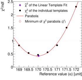
Figure 5: Illustration of various $\chi^{2}/n_{\text{df}}$ values in the scope of the Linear Template Fit for Example 1 (section 4). The red star indicates the best-fit $\chi^{2}$ of the Linear Template Fit, $\hat{\chi}^{2}$. The full circles display the $\chi^{2}$ values of the individual templates and the red line displays the $\chi^{2}$-parabola calculated from them, and its minimum is inicated with an open circle ($\check{\chi}^{2}$, see text).

An alternative best estimator, denoted in the following as $\bm{\check{\alpha}}$, is obtained from the interpretation of all of the $\chi^{2}_{j}$ values, and serves as a validation of the best estimator from the Linear Template Fit ($\bm{\hat{\alpha}}$). Based on the assumption that the $\chi^{2}$ distribution $\chi^{2}(\bm{\alpha})$ follows a second-degree polynomial, the so-called $\chi^{2}$-parabola, its minimum is interpreted as best estimator. For a univariate problem, when introducing

$$\bm{\chi^{2}}=\begin{pmatrix}\chi^{2}_{1}\\ \vdots\\ \chi^{2}_{j}\end{pmatrix}\,,~{}~{}~{}C_{\textrm{(pol-2)}}=\begin{pmatrix}1&\dot{\alpha}_{1}&\dot{\alpha}_{1}^{2}\\ \vdots&\vdots&\vdots\\ 1&\dot{\alpha}_{j}&\dot{\alpha}_{j}^{2}\\ \end{pmatrix}~{}~{}~{}\text{and}~{}~{}~{}\bm{\vartheta}=\begin{pmatrix}\vartheta_{0}\\ \vartheta_{1}\\ \vartheta_{2}\end{pmatrix}\,,$$ (68)

with $\chi^{2}_{j}$ from eq. (67), the best estimator of the model parameter is given by the stationary point of the polynomial

$$\check{\alpha}=\frac{\hat{\vartheta}_{1}}{-2\hat{\vartheta}_{2}}\,,$$ (69)

where the best estimators of the (three) polynomial parameters are $\bm{\hat{\vartheta}}=(C^{\text{T}}C)^{-1}C\bm{\chi^{2}}$. An illustration for Example 1 is shown in figure 5. The uncertainty in $\check{\alpha}$ is given by the criterion $\chi^{2}_{\text{min}}+1$ [10] and hence

$$\sigma_{\check{\alpha}}=\frac{\sqrt{\hat{\vartheta}_{1}^{2}-4\hat{\vartheta}_{2}(\hat{\vartheta}_{0}-\check{\chi}^{2}-1)}}{-2\hat{\vartheta}_{2}}~{}~{}~{}\text{using}~{}~{}~{}\check{\chi}^{2}=(\bm{\chi^{2}}-C\bm{\hat{\vartheta}})^{\text{T}}(\bm{\chi^{2}}-C\bm{\hat{\vartheta}})\,.$$ (70)

The equations for the multivariate case are straightforward and not repeated here. This alternative best estimator, $\check{\alpha}$, as well as its variance $\sigma_{\check{\alpha}}$ and the minimum $\chi^{2}$, should be sufficiently consistent with the results from the Linear Template Fit:

$$\check{\alpha}\sim\hat{\alpha}\,,~{}~{}~{}\sigma_{\check{\alpha}}\sim\sigma_{\hat{\alpha}}~{}~{}~{}\text{and}~{}~{}~{}\check{\chi}^{2}\sim\hat{\chi}^{2}\,,$$ (71)

and may serve as a valuable cross check. As a quick and practical visual test, if the templates line up on the parabolic fit (as seen in figure 5), the problem is essentially linear and the Linear Template Fit will provide an unbiased and optimal best estimator. Note, that for the calculation of eq. (69) at least three templates are required, whereas the minimum number of templates for the univariate Linear Template Fit is only two.

10.4 Power law factor for the linear regression

In the Linear Template Fit the functions $\mathbf{\hat{y}}(\bm{\alpha})$ are (multi-dimensional) linear functions, see eqs. (15), (27), and (38). Although the use of higher-degree polynomials or multivariate polynomials with interference terms could in principle be considered (see next section 11), in such cases the optimization problem cannot be solved analytically and no closed matrix expression for the best estimators is found. However, an analytic solution is still obtained when only power law factors are introduced, and in a univariate Linear Template Fit the model approximation becomes

$$\mathrm{y}_{i}(\alpha;\theta_{0},\theta_{1})=\theta^{(i)}_{0}+\theta^{(i)}_{1}\alpha^{\gamma}$$ (72)

with $\gamma>0$ being a real number. The matrix $M$, eq. (10), then has elements $M_{j,0}=1$ and $M_{j,1}=\dot{\alpha}_{j}^{\gamma}$. In the multivariate case, different power law factors for each fit parameter can be introduced, and one writes $\gamma_{k}$ and has $M_{j,(k+1)}=\dot{\alpha}_{(j),k}^{\gamma_{k}}$. The best estimators of the multivariate Linear Template Fit, eq. (32), then become

$$\hat{\alpha}_{k}=\left(\mathcal{F}(\bm{d}-Y\bm{\bar{m}})\right)_{k}^{\frac{1}{\gamma_{k}}}\,.$$ (73)

This solution can immediately be seen by a variable substitution of $\alpha^{\gamma}$ in eqs. (32) and (72). The application of the power law factor(s) $\gamma$ when working with relative uncertainties (see section 7) is straightforward, since all equations remain linear in $\alpha_{k}$. Similarly, the equations for the error propagation (see section 8) can easily be adopted with that variable substitution. For instance, the elements of the systematic shifts (see eq (43)) become

$$(\bm{\sigma}_{\bm{\hat{a}}}^{(\bm{s}_{(l)})})_{k}=\frac{\left(\mathcal{F}\bm{s}_{(l)}\right)_{k}}{\gamma_{k}\hat{\alpha}_{k}^{\gamma_{k}-1}}\,,$$ (74)

and similarly for other uncertainty components or covariance matrices. The power law factor $\gamma$ may be of practical use in order to validate the assumptions of the linearity of the regression analysis, or to improve the fit, such as when it is known that the model is proportional to $\alpha^{2}$. This would be the case in determinations of the strong coupling constant from $n$-jet production cross sections at the LHC, which are proportional to $\alpha^{n}_{s}(m_{Z})$ at the leading order in perturbative Quantum Chromodynamics (QCD).

10.5 Finite differences

In a use case where a larger number of templates are available, various choices of subsets of these templates can become input to the Linear Template Fit, and some of such potential choices have already been suggested in the previous paragraphs. In the case where only two (or three) templates are provided as input to the Linear Template Fit, the selected templates may have a special meaning, because the templates can also be considered as a numerical first derivative through finite differences. Such numerically calculated derivatives are the essence of many gradient descent optimization methods [5, 87, 50, 86, 49], and it is instructive to study the relation.

As an example, let us consider a univariate problem where the objective function $\chi^{2}$ is given by eq. (8). Close to the minimum, $\chi^{2}$ is nearly quadratic, and the Newton step, $\Delta\alpha=-(\chi^{2})^{\prime}/(\chi^{2})^{\prime\prime}$, exhibits a good convergence [51, 5, 87, 50]. The first and second derivatives at an expansion point $\alpha_{0}$ are

$$(\chi^{2})^{\prime}=-2\bm{\lambda}^{\prime\text{T}}(\alpha_{0})W(\bm{d}-\bm{\lambda}(\alpha_{0}))~{}~{}~{}\text{and}~{}~{}~{}(\chi^{2})^{\prime\prime}=2\bm{\lambda}^{\prime\text{T}}(\alpha_{0})W\bm{\lambda}^{\prime}(\alpha_{0})\,,$$ (75)

where the second derivatives $\bm{\lambda}^{\prime\prime}$ are zero or neglected in the latter equation. Hence, one obtains the estimator from the Newton step as

$$\hat{\alpha}_{\text{(Newton)}}=\alpha_{0}+\left[\bm{\lambda}^{\prime\text{T}}(\alpha_{0})W\bm{\lambda}^{\prime}(\alpha_{0})\right]^{-1}\bm{\lambda}^{\prime\text{T}}(\alpha_{0})W(\bm{d}-\bm{\lambda}(\alpha_{0}))\,,$$ (76)

and the calculation of the first derivative could be done numerically using a finite difference with nonzero step size $h$

$$\bm{\lambda}^{\prime}(\alpha_{0})=\frac{\bm{\lambda}(\alpha_{0}+h)-\bm{\lambda}(\alpha_{0})}{h}\,.$$ (77)

The analogous Linear Template Fit makes use of the templates at $\alpha_{0}$ and $\alpha_{0}+h$ and defines the following matrices

$$Y=\begin{pmatrix}\bm{\lambda}(\alpha_{0})&~{}\bm{\lambda}(\alpha_{0}+h)\end{pmatrix}~{}~{}\text{and}~{}~{}M=\begin{pmatrix}1&\alpha_{0}\\ 1&~{}\alpha_{0}+h\end{pmatrix}\,,~{}\text{hence}~{}M^{+}=\begin{pmatrix}\tfrac{\alpha_{0}+h}{h}&-\tfrac{\alpha_{0}}{h}\\ -\tfrac{1}{h}&\tfrac{1}{h}\end{pmatrix}=\begin{pmatrix}\bm{\bar{m}}^{\text{T}}\\ \bm{\tilde{m}}^{\text{T}}\end{pmatrix}\,.$$ (78)

From the Linear Template Fit, eq. (17), when resolving $\bm{\bar{m}}$, one obtains the best estimator

$$\hat{\alpha}=\alpha_{0}+\left[(Y\bm{\tilde{m}})^{\text{T}}W(Y\bm{\tilde{m}})\right]^{-1}(Y\bm{\tilde{m}})^{\text{T}}W(\bm{d}-\bm{\lambda}(\alpha_{0}))$$ (79)

and since $Y\bm{\tilde{m}}=\bm{\lambda}^{\prime}(\alpha_{0})$, it can be directly seen that it is equivalent to the estimator $\hat{\alpha}_{\text{(Newton)}}$ from the Newton step using a numerical finite difference.

11 Nonlinear model approximation

The Linear Template Fit can be regarded such that linear functions are fitted to every row $i$ of the template matrix $Y$. In the following, nonlinear functions are considered for the model $\lambda_{i}(\bm{\alpha})$ in each “bin” $i$. For a simplified discussion, the formuluae for only a univariate model are sometimes discussed, while the multivariate case is commonly straightforward. Also, the concepts of the $\gamma$ factor, relative uncertainties, or “systematic shifts” $\bm{s}_{l}$ can equally be considered in a multivariate formulation.

The model can be approximated from the templates in every bin $i$ with an $n$th degree polynomial function

$$\lambda_{i}(\alpha)\approx\mathrm{y}_{i}(\alpha;\bm{\hat{\theta}}_{(i)})=:\hat{\mathrm{y}}_{i}(\alpha)~{}~{}~{}\text{using}~{}~{}~{}\mathrm{y}_{i}(\alpha;\bm{\theta}_{(i)})=\theta_{0}^{(i)}+\theta_{1}^{(i)}\alpha+\ldots+\theta_{n}^{(i)}\alpha^{n}\,.$$ (80)

The best estimators for the polynomial parameters are obtained from regression analysis,

$${\bm{\hat{\theta}}_{(i)}}=\left(\begin{smallmatrix}\hat{\theta}_{0}\\ \hat{\theta}_{1}\\ \vdots\\ \hat{\theta}_{n}\end{smallmatrix}\right)_{(i)}=\mathcal{M}^{+}\begin{pmatrix}y_{(1),i}\\ \vdots\\ y_{(j),i}\end{pmatrix}\,,$$ (81)

where $y_{(j),i}$ is the $i$th value of the $j$th template, and the $g$-inverse is

$$\mathcal{M}^{+}=\left(\mathcal{M}^{\text{T}}\mathcal{M}\right)^{-1}\mathcal{M}^{\text{T}}~{}~{}~{}~{}\text{using here}~{}~{}~{}~{}\mathcal{M}=\begin{pmatrix}1&\dot{\alpha}_{1}&\ldots&\dot{\alpha}_{1}^{n}\\ \vdots&\vdots&\vdots&\vdots\\ 1&\dot{\alpha}_{j}&\ldots&\dot{\alpha}_{j}^{n}\\ \end{pmatrix}\,.$$ (82)

For reasons outlined in section 3 an unweighted regression is considered. Using this model approximation in the objective function of the fitting problem, eq. (2), the $\chi^{2}$ expression for a univariate model becomes of order $\mathcal{O}(2n)$ in $\alpha$,

$$\chi^{2}_{\mathcal{O}{(2n)}}: =\left(\bm{d}-\bm{\hat{\mathrm{y}}}(\alpha)\right)^{\text{T}}W\left(\bm{d}-\bm{\hat{\mathrm{y}}}(\alpha)\right)$$ (83)

$$=\left(\bm{d}-Y\bm{m_{0}}-Y\bm{m_{1}}\alpha-\ldots-Y\bm{m_{n}}\alpha^{n}\right)^{\text{T}}W\left(\bm{d}-Y\bm{m_{0}}-Y\bm{m_{1}}\alpha-\ldots-Y\bm{m_{n}}\alpha^{n}\right)\,,$$ (84)

where the vectors $\bm{m}$ were used as the representation of $\mathcal{M}^{+}$ according to

$$\mathcal{M}^{+}=:\left(\begin{smallmatrix}\bm{m_{0}}^{\text{T}}\\ \bm{m_{1}}^{\text{T}}\\ \vdots\\ \bm{m_{n}}^{\text{T}}\\ \end{smallmatrix}\right)\,.$$ (85)

It is obvious that for $n=1$, this is the Linear Template Fit, and the generalizations to the multivariate fit (eq. (30)), and with relative uncertainties (eq. (39)), are straightforward. Note that for different degrees $n$, the vectors $\bm{m}$ differ unless the equations are not rewritten for orthogonal polynomials [93].

Since the first derivative of $\chi^{2}_{\mathcal{O}{(2n)}}$ is nonlinear in $\alpha$, no analytic solution of the optimization problem is found. Therefore, in the following, two iterative algorithms to find the minimum of the objective function $\chi^{2}_{\mathcal{O}{(2n)}}$ are discussed, which refer to the Gauß–Newton and the Newton algorithm (see also Refs. [51, 5, 87, 50]). In both cases, if the starting value is identified with the best estimator from the Linear Template Fit, $\alpha=\hat{\alpha}$, the step size of the next iterative step can be interpreted as convergence criterion or uncertainty of the Linear Template Fit. Reasonable values for $n$ are $n=2$, 3, or at most 4 (since $\mathcal{M}$ becomes quickly ill-conditioned for large $n$, e.g. Refs. [94, 95] and therein), while for $n=1$, consistent results with the Linear Template Fit are found.

11.1 Linearization of the nonlinear approxmation $\hat{\mathrm{y}}(\alpha)$

An iterative minimization algorithm based on first derivatives is defined through linearly approximating the (nonlinear) function $\bm{\hat{\mathrm{y}}}(\alpha)$, eq. (80). For the purpose of validating the result from the Linear Template Fit, we consider $\hat{\alpha}$ as the expansion point, although this could be any other value as well. Hence, the linear approximation of $\bm{\hat{\mathrm{y}}}(\alpha)$ in every bin $i$ is

$$\tilde{y}_{i}(\alpha) \approx\hat{\mathrm{y}}_{i}(\hat{\alpha})+\left.\frac{\partial\hat{\mathrm{y}}_{i}(\alpha)}{\partial\alpha}\right|_{\alpha=\hat{\alpha}}(\alpha-\hat{\alpha})$$

$$=Y(\textstyle{\sum}_{0}^{n}(1-n)\bm{m}_{(n)}\hat{\alpha}^{n})+Y\left(\textstyle{\sum}_{0}^{n}n\bm{m}_{(n)}\hat{\alpha}^{n-1}\right)\alpha$$

$$=:Y\bm{\tilde{\bar{m}}}+Y\bm{\tilde{\tilde{m}}}\alpha\,.$$ (86)

The last term defines the shorthand notations $\bm{\tilde{\bar{m}}}$ and $\bm{\tilde{\tilde{m}}}$. From comparison with eq. (15), it is seen that an alternative best estimator of the template fit (see eq. (19)) is obtained as

$$\tilde{\hat{\alpha}}=\frac{(Y\bm{\tilde{\tilde{m}}})^{\text{T}}W}{(Y\bm{\tilde{\tilde{m}}})^{\text{T}}WY\bm{\tilde{\tilde{m}}}}(\bm{d}-{Y\bm{\tilde{\bar{m}}}})\,.$$ (87)

The difference $\hat{\alpha}-\tilde{\hat{\alpha}}$ is supposed to become small for a valid application of the Linear Template Fit, and one should find

$$|\hat{\alpha}-\tilde{\hat{\alpha}}|\ll\sigma_{\hat{\alpha}}\,.$$ (88)

If eq. (88) holds for a particular application, then nonlinear effects are negligible, and the best estimator of the Linear Template Fit is insensitive to nonlinear effects in the model $\lambda$. If eq. (88) does not hold, then it should be studied if the nonlinearity is present in the vicinity of $\hat{\alpha}$ or if it is rather introduced by a long-range nonlinear behavior of $\lambda(\alpha)$. In the latter case, the range of the templates should be reduced such that one has about

$$\dot{\alpha}_{\text{max}}-\dot{\alpha}_{\text{min}}\lesssim 2\sigma_{\hat{\alpha}}\,$$ (89)

and the Linear Template Fit should be repeated. Note that if the templates are subject to statistical fluctuations and if only a few templates are provided, then a nonlinear approximation is more sensitive to those fluctuations than linear approximations, and $|\hat{\alpha}-\tilde{\hat{\alpha}}|$ may become larger. In such an application $\sigma_{\hat{\alpha}}^{Y}$ should also be considered as a relevant source of uncertainty (see eqs. (46) and (47)).

In Example 1, when using a second-degree polynomial, a value $|\hat{\alpha}-\tilde{\hat{\alpha}}|=0.02$ is found, which is much smaller than $\sigma_{\hat{\alpha}}=\pm 0.41$ and of similar size than the statistical uncertainties from $Y$ (see section 8.5). When working with log-normal uncertainties, a value $|\hat{\alpha}-\tilde{\hat{\alpha}}|=0.05$ is found. Although the model is highly nonlinear in $\log(y)$, the assumptions of the linear template fit are well justified since the templates are in the close vicinity of the best estimator. In Example 2, for a second degree approximation values of $|\hat{\alpha}_{0}-\tilde{\hat{\alpha}}_{0}|=0.03$ and $|\hat{\alpha}_{1}-\tilde{\hat{\alpha}}_{1}|=0.14$ are found. When further considering interference terms, see Appendix C, the values are $0.01$ and $0.11$, respectively All these values are smaller than the respective statistical uncertainties in the data, although the values suggest that for $\alpha_{1}$ (the variance of the gaussian model) a finer grid for the reference values may be preferred, for a more accurate linear approximation.

Furthermore, the notation of eq. (86) suggests an alternative interpretation of the non-linear behaviour of the model. The vectors $\bm{\tilde{\bar{m}}}$ and $\bm{\tilde{\tilde{m}}}$ may be interpreted in terms of uncertainties of $\bm{\bar{{m}}}$ and $\bm{\tilde{{m}}}$ when writing

$$\bm{\sigma}_{\bm{\bar{{m}}}}:=\bm{\tilde{\bar{m}}}-\bm{\bar{{m}}}~{}~{}~{}~{}\text{and}~{}~{}~{}~{}\bm{\sigma}_{\bm{\tilde{{m}}}}:=\bm{\tilde{\tilde{m}}}-\bm{\tilde{{m}}}\,.$$ (90)

Through linear error propagation, one can define an uncertainty in $\hat{\alpha}$ as

$$\sigma_{\hat{\alpha}}^{(m)} =\sum_{j}\bigg{(}-FY\mathbb{1}_{j}\sigma_{\bar{m}_{j}}+D^{-1}\left[(Y\mathbb{1}_{j})^{\text{T}}W(d-Y\bar{m})-\left[(Y\mathbb{1}_{j})^{\text{T}}WY\tilde{m}+(Y\tilde{m})^{\text{T}}WY\mathbb{1}_{j}\right]\hat{a}\right]\sigma_{\tilde{m}_{j}}\bigg{)}$$

$$=\sum_{i}\bigg{(}-F\mathbb{1}_{i}\sigma_{\overline{Ym}_{i}}+D^{-1}\big{[}\mathbb{1}_{i}^{\text{T}}W(d-Y\bar{m})-\left[\mathbb{1}_{i}^{\text{T}}WY\tilde{m}+(Y\tilde{m})^{\text{T}}W\mathbb{1}_{i}\right]\hat{a}\big{]}\sigma_{\widetilde{Ym}_{i}}\bigg{)}\,.$$ (91)

Note that the sum runs over $j$ in the first and over $i$ in the second expression. The second expression makes use of

$$\bm{\sigma}_{\bm{\overline{Ym}}}:=Y\bm{\sigma}_{\bm{\bar{m}}}~{}~{}~{}~{}\text{and}~{}~{}~{}~{}\bm{\sigma}_{\bm{\widetilde{Ym}}}:=Y\bm{\sigma}_{\bm{\tilde{{m}}}}$$ (92)

and it has the advantage that the summands represent a useful quantifier for every bin $i$. For a sufficiently linear problem, both the linear sum (eq. (91)) and the quadratic sum should be sufficiently small. In particular, one should find $\sigma_{\hat{\alpha}}^{(m)}\approx\tilde{\hat{\alpha}}-\hat{\alpha}$ for reasonable $n$th degree polynomials, i.e. $n$=2, and also, according to eq. (88),

$$|\sigma_{\hat{\alpha}}^{(m)}|\ll|\sigma_{\hat{\alpha}}|\,.$$ (93)

11.2 Minimization of $\chi^{2}_{\mathcal{O}{(2n)}}$

When $\hat{\alpha}$ is obtained from the Linear Template Fit, the objective function $\chi^{2}_{\mathcal{O}{(2n)}}$, eq. (84), is expected to exhibit a minimum in the close vicinity of $\hat{\alpha}$. This provides good motivation for the application of the Newton optimization at $\hat{\alpha}$, which is based on second derivatives of $\chi^{2}_{\mathcal{O}{(2n)}}$, so a parabolic approximation. The Newton distance to the minimum is given by

$$\Delta\alpha=-\frac{(\chi^{2}_{\mathcal{O}{(2n)}})^{\prime}}{(\chi^{2}_{\mathcal{O}{(2n)}})^{\prime\prime}}=-\left(\left.\frac{\partial^{2}\chi^{2}_{\mathcal{O}{(2n)}}}{\partial^{2}\alpha}\right|_{\alpha=\hat{\alpha}}\right)^{-1}\left.\frac{\partial\chi^{2}_{\mathcal{O}{(2n)}}}{\partial\alpha}\right|_{\alpha=\hat{\alpha}}$$ (94)

and in the multivariate case by [55, 5]

$$\bm{\Delta\alpha}=\left.-H^{-1}\bm{g}\right|_{\bm{\alpha}=\bm{\hat{\alpha}}}\,.$$ (95)

The gradient vector $\bm{g}$ and the Hesse matrix $H$ are defined by the first and second derivatives of $\chi^{2}_{\mathcal{O}{(2n)}}$, respectively. Both quantities can be calculated directly at an expansion point $\bm{\alpha_{0}}$, which was identified in the above equations with $\bm{\hat{\alpha}}$, since $\chi^{2}_{\mathcal{O}{(2n)}}$ is just a known second-degree polynomial and dependent on $M$, $Y$, $\bm{d}$, $S$, and $W$. The value of $\bm{\Delta\alpha}$ can be interpreted as the expected distance to the minimum (EDM) based on the nonlinear model approximation.

For practical purposes and to validate the result of the Linear Template Fit one should require that its value be smaller than the uncertainty from the fit

$$|\Delta\alpha|\ll\sigma_{\hat{\alpha}}\,.$$ (96)

The most reasonable degree for this purpose is $n=2$ (which is exploited in the following in greater detail), and one expects that $\Delta\alpha$ will be negligibly small. This observation can also be interpreted such that the result from the Linear Template Fit and an alternative result from a minimization of $\chi^{2}_{\mathcal{O}{(2n)}}$ are consistent. If the reference points are in the vicinity of $\hat{\alpha}$, this is to be expected because of the underlying statistical model of (log-)normal distributed estimators. In contrast, if $\Delta\alpha$ becomes large, it may well be that in such a case not even the reported uncertainties in the best estimator, $\sigma_{\hat{\alpha}}$, can be considered to be normal distributed.

12 The Quadratic Template Fit

Despite all the considerations and cross-checks as discussed in the previous sections, in some problems the linearized model may simply be an inaccurate approximation of the true model (cf. eq. (27)). Reasons could be that the templates cannot be generated in a sufficiently close vicinity around the best estimator, perhaps for technical reasons, or in multivariate problems some parameters are highly nonlinear, a dimension is poorly constrained and the reference points span a large range, or interference terms between the parameters are non-negligible. In such cases, the quantities $\bm{\tilde{\hat{\alpha}}}-\bm{\hat{\alpha}}$, $\bm{\sigma_{\hat{\alpha}}^{(m)}}$, or $\bm{\Delta\alpha}$ (eqs. (88), (91) and (95)) become non-negligible when they are calculated for second-degree polynomials $n=2$.

An improved approximation of the model is obtained when using a second order approximation, which may also include interference terms. The equations are summarized in Appendix C (eqs. (103)–(105)). Using such a second-degree polynomial model $\bm{\hat{\mathrm{y}}}(\bm{\alpha})$ that includes terms $\mathcal{O}(\alpha_{k})$, $\mathcal{O}(\alpha^{2}_{k})$, and $\mathcal{O}(\alpha_{k_{1}}\alpha_{k_{2}})$ in the optimization problem results in a nonlinear least-squares problem. Therefore, an iterative algorithm is required to obtain the best estimator.

A robust algorithm, denoted as Quadratic Template Fit, to obtain the best estimator and to perform a full error propagation is defined as

1. The Linear Template Fit is performed to obtain a first estimator $\bm{\hat{\alpha}}_{(0)}$, for example using eq. (32);

2. The Newton algorithm [51, 5, 87, 50], eq. (95), is employed with a few $m$ iterations in order to obtain improved best estimators $\bm{\hat{\alpha}}_{(m)}=\bm{\hat{\alpha}}_{(m-1)}+\bm{\Delta\alpha}_{(m)}$ and for which the Hesse matrix $H$ is directly analytically calculable;

3. The best estimator and the error calculation are obtained using the linearized approximations for $\bm{\tilde{\bar{m}}}$ and $\tilde{\tilde{M}}$ (see eqs. (86) or (109)) in the equations of the Linear Template Fit.

The first step provides the starting point for the Newton algorithm, and since it is obtained with the Linear Template Fit it is already close to the minimum. The second step provides a fast and stable convergence since the starting point is already in the vicinity of the minimum, the Hesse matrix is commonly positive definite and is analytically exactly calculable,, as well as the gradient vector, and the Newton method has good convergence for nearly quadratic functions [51, 5, 50], which is the case for $\chi^{2}_{\mathcal{O}{(4)}}$. Although the algorithm is expected to converge quickly after a very few iterations, several stopping criteria are thinkable, for example when EDM$\ll|\bm{\Delta\alpha}|$ or $\bm{\Delta\alpha}_{(m)}\approx\bm{\Delta\alpha}_{(m-1)}$. The last step provides an even more improved best estimator, but mainly gives access to the equations of the error propagation. Note that in the first step, the true model $\bm{\lambda}(\bm{\alpha})$ is linearly approximated, and in the latter steps, by quadratic functions.

When applying the Quadratic Template Fit to Example 2, and using $m=2$ Newton-iterations, the best estimator for the mean is found to be $169.90\pm 0.44$ and for the variance it is $6.23\pm 0.32$. Both values are very close to the best estimators from the Linear Template Fit, see section 6. The EDM $\bm{\Delta\alpha}$ and $\bm{\tilde{\hat{\alpha}}}-\bm{\hat{\alpha}}$ are found to be smaller than $10^{-4}$ for both parameters, and $\bm{\sigma}_{\bm{\hat{\alpha}}}^{(m)}$ is equally small.

13 Example 3: the Quadratic Template Fit

As an application of the Quadratic Template Fit, an example is constructed where the model is nonlinear and the templates purposefully span a (too) large range. Therefore, the criteria for a valid application of the Linear Template Fit as discussed in section 10 are mainly not fulfilled.

As in Example 1 and 2 (sections 4 and 6), the model is considered to be a normal distribution, and the same pseudo-data as in the previous examples are also used. In contrast to Examples 1 and 2, only the variance of the normal distribution shall be determined. Six templates are generated similarly to Examples 1 and 2, with variances between 3 and 8, and each template is generated using $4\cdot 10^{6}$ events. The pseudo-data and the templates are displayed in figure 6. Recall that the pseudo-data were generated with a variance of 6.2 (due to statistical fluctuations, the true variance is about 6.3).

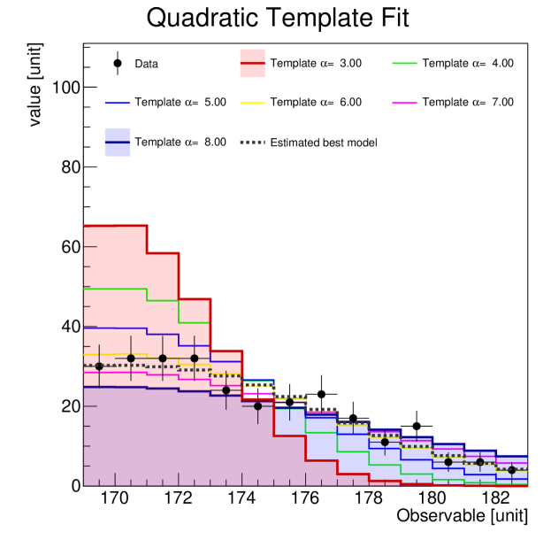
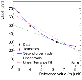
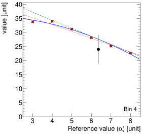
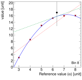
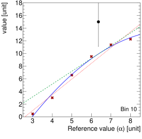
Figure 6: Some illustrations of Example 3. Left: the template distributions $Y$ as a function of the observable, and more details are given in the caption of figure 1. Right: the templates $Y$ for some selected bins. The blue line indicates a second-degree polynomial regression of the templates, as is used by the Quadratic Template Fit. The green dashed line indicates the linearization at the best estimator, and the red dotted line indicates the linear regression of the templates as it would be used by the plain Linear Template Fit.

In this example, the Linear Template Fit results in a best estimator of $6.61\pm 0.32$, and is thus not quite consistent with the expectation. The EDM is comparably large, with a value of $-0.27$ , and $\sigma_{\hat{\alpha}}^{(m)}=-0.27$, and the minimum of the $\chi^{2}$-parabola results in $6.52\pm 0.27$. Consequently, eqs. (61), (62), (71), and (93) are not well fulfilled. In figure 6 (right), the parameter dependence in some selected bins is displayed, and it is clearly seen that the templates are not described by a linear function. It is also observed from the $\chi^{2}$ values of the individual templates that these cannot be described by a parabola as would be the case for a linear problem, as displayed in figure 7.

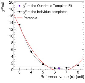
Figure 7: Visualization of the $\chi^{2}$ values of the templates in Example 3. A thin line connects these values. The red line displays a fitted parabola, which is not able to describe the $\chi^{2}$ values adequately, which is indicative of a nonlinear problem. The star indicates the best estimator from the Quadratic Template Fit.

The Quadratic Template Fit, in contrast, results in a best estimator of $6.36\pm 0.40$ and is thus in excellent agreement with the expectation. This is because the algorithm employs a second-degree polynomial in each bin to represent the model. This provides an adequate representation of the parameter dependence even of a nonlinear model, as also seen in figure 6 (right). A linearization at the value of the best estimator is used only for linear error propagation, and appears to be appropriate given the size of the final uncertainties, $\pm 0.40$.

14 Validation study: determination of the strong coupling constant from inclusive jet cross section data

As an example application of the Linear Template Fit, the strong coupling constant in Quantum Chromodynamics (QCD), $\alpha_{\rm s}(m_{\rm Z})$, is determined from a measurement of inclusive jet cross sections in proton–proton collisions at a center-of-mass energy of $\sqrt{s}=7\,$TeV [96]. The data were taken with the CMS detector at the LHC at CERN. Inclusive jets were measured as a function of the transverse momentum $p_{\text{T}}$ in five regions of absolute rapidity $|y|$. Altogether 133 data points are available, and 24 different sources of uncertainties are associated with the data.

The model is obtained from a calculation in next-to-leading order perturbative QCD (NLO pQCD) using the program nlojet++ [97, 98] that was interfaced to the tool fastNLO [99, 100, 101]. The latter makes it possible to provide templates for any value of $\alpha_{\rm s}(m_{\rm Z})$ and different parameterizations of parton distribution functions of the proton (PDFs) without rerunning the calculation of the pQCD matrix elements. Multiplicative non-perturbative (NP) [102] and electroweak corrections [103] are applied to the NLO predictions.

The value of $\alpha_{\rm s}(m_{\rm Z})$ was already determined earlier from these data and in NLO accuracy in two independent analyses [104, 105]. The two analyses differ in the assumption of the statistical model, the inference algorithm, and the uncertainties considered in the fit. This provides a comprehensive testing ground to compare the results from the Linear Template Fit.

In Ref. [104], the value of $\alpha_{\rm s}(m_{\rm Z})$ is determined from the minimum of a $\chi^{2}$-parabola, where the $\chi^{2}$ is derived from normal distributed probability distribution functions. In order to avoid a bias in that procedure [69, 68, 64], some uncertainty components are treated as multiplicative [104], which means that the covariance matrix is calculated from relative uncertainties that are multiplied with theory predictions. We chose predictions obtained with $\alpha_{\rm s}(m_{\rm Z})=0.116$ for that purpose, and the total covariance matrix in $\chi^{2}$ is calculated as described in Ref. [104].

The templates are generated in the range $0.112\leq\alpha_{\rm s}(m_{\rm Z})\leq 0.121$ in steps of 0.001 using the MSTW PDF set [106]. In this methodology, the model predictions are not available for continuous values of $\alpha_{\rm s}(m_{\rm Z})$, since the PDFs als exhibit an $\alpha_{\rm s}$ dependence, but are provided only in a limited range and for discrete $\alpha_{\rm s}(m_{\rm Z})$ values [106]. Therefore, this kind of $\alpha_{\rm s}(m_{\rm Z})$ inference is a typical use case for the Linear Template Fit The templates and the linear model are displayed for some selected bins in figure 8.

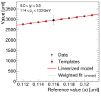
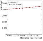
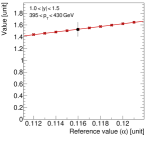
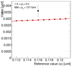
Figure 8: Visualization of the templates, the data, and the implicit linearization of the model in some selected bins of the Linear Template Fit to the CMS inclusive jet cross sections. More details are given in the caption of figure 1.

Fit method	Best estimator $\alpha_{\rm s}(m_{\rm Z})$	$\chi^{2}$/$n_{\rm dof}$
Linear Template Fit	$0.1159\pm 0.0014_{\text{(exp)}}\pm 0.0011_{\text{(pdf)}}\pm 0.0001_{\text{(NP)}}$	$107.4/132$
Quadratic Template Fit	$0.1160\pm 0.0014_{\text{(exp)}}\pm 0.0011_{\text{(pdf)}}\pm 0.0001_{\text{(NP)}}$	$107.2/132$
$\chi^{2}$-parabola	$0.1160\pm 0.0018_{\text{(exp,PDF)}}$	$107.2/132$
CMS [104]	$0.1159\pm 0.0012_{\text{(exp)}}\pm 0.0014_{\text{(pdf)}}\pm 0.0001_{\text{(NP)}}$	$107.2/132$

Table 1: The results from a Linear Template Fit of NLO pQCD predictions using the MSTW PDF set to CMS inclusive jet cross section data. The results are compared with the Quadratic Template Fit and to the analytic calculation of the minimum of the $\chi^{2}$-parabola, as well as to the published results by the CMS collaboration in the last row. Shown are the best estimators for $\alpha_{\rm s}(m_{\rm Z})$, the quadratic sum of all experimental uncertainties (exp), the propagated PDF uncertainties (PDF), the propagated NP uncertainties (NP), and the last column shows the $\chi^{2}$/$n_{\rm dof}$ values. The difference between the Linear and the Quadratic Template Fit is only $0.000017$, but appears larger due to a rounding effect. Differences to the CMS result may also be due to numerical limitations of the input data, or how the PDF uncertainties are symmetrized. The total uncertainties that are considered in the fit sum to $\pm 0.0018$ in all cases.

The results from the Linear Template Fit (eq. (32)), the Quadratic Template Fit (section 12), and the parabolic fit (section 10.3) are compared with the published results from CMS in table 1. An illustration of the $\chi^{2}$ values is displayed in figure 9 (left).

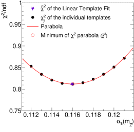
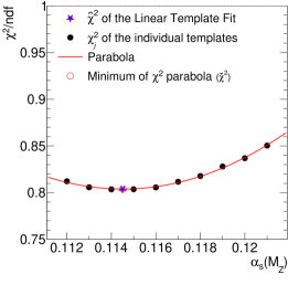
Figure 9: Illustration of $\chi^{2}$/$n_{\rm dof}$ values in the fit of NLO pQCD predictions to CMS inclusive jet cross section data. Shown are the $\chi^{2}$/$n_{\rm dof}$ value of the Linear Template Fit at its best estimator (star), the $\chi^{2}$/$n_{\rm dof}$ values of the individual templates (full circle), and the calculated $\chi^{2}$ parabola (see sect. 10.3) and its minimum (open circle). Left: $\chi^{2}$/$n_{\rm dof}$ values of the Linear Template Fit with normal-distributed uncertainties. Right: $\chi^{2}$/$n_{\rm dof}$ values of the linear template with log-normal distributed uncertainties. Note that the left figure uses the PDF set MSTW for the NLO predictions with a varying $\alpha_{\rm s}(m_{\rm Z})$ value, whereas the right one uses the PDF set NNPDF3.0.

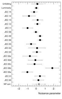
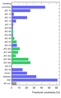
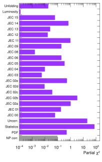
Figure 10: Left: nuisance parameters of the systematic uncertainties in the $\alpha_{\rm s}(m_{\rm Z})$-fit to CMS inclusive jet cross section data. Details on these uncertainties are found in Refs. [96, 104]. The gray value(s) are not included in the $\chi^{2}$ computation but are propagated separately. Middle: size of the individual uncertainty components to the total uncertainty of the best estimator, $\alpha_{\rm s}(m_{\rm Z})$, in the Linear Template Fit to CMS inclusive jet cross section data. The color indicates the sign of the uncertainty, which, however, is of relevance only for multivariate fits. Right: partial $\chi^{2}$ from the individual uncertainty components.

The best estimator for $\alpha_{\rm s}(m_{\rm Z})$, its uncertainties, and the value of $\chi^{2}$ are in good agreement among each other, and with the published CMS values [104], and differences are only in the rounding digit. It is also found that the total “fit” uncertainty is reproduced, which comprises the experimental and the PDF uncertainties, $\delta\alpha_{\rm s}(m_{\rm Z})=\delta\alpha_{\rm s}^{\text{(exp)}}\oplus\delta\alpha_{\rm s}^{\text{(PDF)}}=\pm 0.0018$. The small differences in the individual uncertainty components between Ref. [104] and the Linear Template Fit are likely because the error breakdown in Ref. [104] is only approximate, whereas the Linear Template Fit provides an analytic error propagation at the value of the best estimator. In fact, all 24 uncertainty components of the data, the 20 symmetrized PDF uncertainties, and the NP uncertainties are propagated separately (cf. section 8) and are displayed in figure 10. It is observed that the largest individual experimental uncertainty source is the luminosity uncertainty and the statistical uncertainty. The nuisance parameters are quite similar to those from (yet another) fit in Ref. [104]. The uncertainty component with the largest contribution to the total uncertainty stems from the PDFs and the luminosity uncertainty. The statistical and uncorrelated uncertainties have the largest contribution to $\hat{\chi}^{2}$. The NP uncertainties are not included in the nominal $\chi^{2}$ computation and are propagated separately. The EDM of the Linear Template Fit is $7\cdot 10^{-5}$ and thus smaller than the rounding digit of the result.

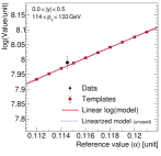
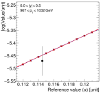
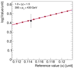
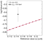
Figure 11: Similar visualization of the templates than in figure 8, but using relative uncertainties (log-normal distributed probability distribution functions) in the Linear Template Fit.

In Ref. [105], as an intermediate result, the value of $\alpha_{\rm s}(m_{\rm Z})$ was determined from CMS inclusive jet cross sections as well. In contrast to Ref. [104], the estimators are assumed to follow a log-normal distribution, and some theoretical uncertainties are further considered in the $\chi^{2}$ expression, which was then minimized with Minuit [4]. The NNPDF3.0 PDF sets [107] are used for the NLO predictions and provide a covariance matrix with PDF uncertainties. This inference provides a useful testing ground for the Linear Template Fit with relative uncertainties (section 7). Templates are generated in the range $0.112\leq\alpha_{\rm s}(m_{\rm Z})\leq 0.121$, and the same uncertainty components as in Ref. [105] are considered. Some selected bins are displayed in figure 11. The results from the Linear Template Fit (eq. (41)), the Quadratic Template Fit, and the parabolic fit are compared with the published results in table 2, and an illustration of $\chi^{2}$ values, which here are calculated from normal-distributed relative uncertainties (eq. (39)), is displayed in figure 9 (right).

Fit method	Best estimator $\alpha_{\rm s}(m_{\rm Z})$	$\chi^{2}$/$n_{\rm dof}$
Linear Template Fit	$0.1144\pm 0.0024_{\text{(exp)}}\pm 0.0011_{\text{(pdf)}}\pm<$$0.0001_{\text{(NP)}}$	$106.1/132$
Quadratic Template Fit	$0.1145\pm 0.0024_{\text{(exp)}}\pm 0.0011_{\text{(pdf)}}\pm<$$0.0001_{\text{(NP)}}$	$106.1/132$
$\chi^{2}$-parabola	$0.1145\pm 0.0026_{\text{(exp,PDF)}}$	$106.1/132$
Ref. [105]	$0.1144\pm 0.0022_{\text{(exp)}}\pm 0.0014_{\text{(pdf)}}\pm 0.0001_{\text{(NP)}}$	0.81

Table 2: Results from a Linear Template Fit with relative uncertainties where NLO pQCD predictions using the NNPDF3.0 PDF set are fitted to CMS inclusive jet cross section data. The results are compared with the Quadratic Template Fit and to the analytic calculation of the minimum of the $\chi^{2}$ parabola, and to previously published results in the last row. Shown are the best estimators for $\alpha_{\rm s}(m_{\rm Z})$, the quadratic sum of all experimental uncertainties (exp), the propagated PDF uncertainties (PDF), the propagated NP uncertainties (NP), and the last column shows the $\chi^{2}$/$n_{\rm dof}$ values.

The best estimator, the uncertainties, and the value of $\chi^{2}$ are in good agreement among each other and with the result from Ref. [105]. The results differ only in the rounding digit, and different sizes of the uncertainty breakdown (into (exp), (PDF), and (NP) uncertainties) may be explained since the error breakdown in Ref. [105] is only approximate, but the total uncertainty is consistently $\delta\alpha_{\rm s}=\pm 0.0026$.

It is worth noting that due to the application of the factorization theorem [108], both the hard coefficients and the PDFs exhibit an $\alpha_{\rm s}$ sensitivity. Consequently, in the two approaches discussed above, not only is the value of $\alpha_{\rm s}(m_{\rm Z})$ determined, but the PDFs are determined simultaneously as well [109], which is realized through the inclusion of the PDF uncertainties in the Linear Template Fit, and which is commonly referred to as PDF profiling. This technique avoids a possible bias that is present when the PDFs are kept fixed [110], and it is particularly valid since the PDFs and the value of $\alpha_{\rm s}(m_{\rm Z})$ are only weakly correlated in PDF determinations, and thus their correlations are negligible [111]. The different size of the uncertainties in tables 1 and 2 is then a consequence of how the PDFs are considered in the fit. Since the PDFs themselves are determined from data as well, the ansatz from CMS also exploits, to some extent, the $\alpha_{\rm s}$ sensitivity of these further data by using the $\alpha_{\rm s}$ dependent PDF, whereas the other ansatz from Ref. [105] exploits only the jet data and their sensitivity to $\alpha_{\rm s}(m_{\rm Z})$ in the hard coefficients.

Consequently, these examples represent a comprehensive application of the Linear Template Fit, where in addition to determining the value of $\alpha_{\rm s}(m_{\rm Z})$, a PDF profiling is also performed, as well as a simultaneous constraint of the systematic uncertainties. Such constraints are obtained when the uncertainties in the nuisance parameters become smaller than unity. A PDF determination from these data alone, instead of a PDF profiling of an existent PDF, would be possible by considering the PDF uncertainties as unconstrained uncertainties in the Linear Template Fit, as described in section 8.4. Such a fit exploits the PDF parameter space of the PDF set that is used to derive the PDF uncertainties. For the given example of CMS inclusive jet cross sections, however, this is not possible, since these data do not have sufficient constraints on the separate PDF flavors.

15 Summary and conclusions

In this article, the equations of the Linear Template Fit were presented. The Linear Template Fit provides an analytic expression for a maximum likelihood estimator in a uni- or multivariate parameter estimation problem. The underlying statistical model is constructed from normal or log-normal probability distribution functions and refers to a maximum likelihood or a minimum $\chi^{2}$ method. For parameter estimation with the Linear Template Fit, the model needs to be provided at a few reference values in the parameter(s) of interest: the templates. The multivariate Linear Template Fit can be written as

$$\bm{\hat{\alpha}}=\left((Y\tilde{M})^{\text{T}}WY\tilde{M}\right)^{-1}(Y\tilde{M})^{\text{T}}W(\bm{d}-Y\bm{\bar{m}})\,,$$

where $Y$ is the template matrix, $\bm{d}$ is the data vector (random vector), $W$ is the inverse covariance matrix, and $\bm{\bar{m}}$ and $\tilde{M}$ are calculated from the reference points (eq. (26)).

The equation of the Linear Template Fit is derived using two key arguments: (i) in the vicinity of the best estimator the model is linear, and (ii) the templates for different reference values are all generated in the same manner. The first precondition is commonly justified if the templates are provided within a reasonably small range around the (to be expected) best estimator. From the second, it follows that the bin-wise polynomial regression is unweighted, and thus the identical regression matrix is applicable in all bins. Several quantities to validate the applicability of the Linear Template Fit in a particular application were discussed.

If the linearity of the model is not justified, the Quadratic Template Fit is a suitable alternative algorithm for parameter estimation. It considers second-degree polynomials for the parameter dependence of the model and employs the quickly converging exact Newton minimization algorithm. For error propagation, the equations of the Linear Template Fit are applicable.

Both the Linear and the Quadratic Template Fit implicitly transform the discrete representation of the model (the templates) into analytic continuous functions using polynomial regression. These expressions themselves may also become useful in several other applications where templates are available but continuous functions would be needed.

The equations for error propagation of different sources of uncertainties were presented. The analytic nature of the Linear Template Fit allows the straightforward propagation of each uncertainty component separately, which provides additional insights into the parameter estimation analysis.

As an example application, previously published results on the determination of the strong coupling constant $\alpha_{\rm s}(m_{\rm Z})$ from inclusive jet cross section data taken at the LHC were repeated. The Linear and the Quadratic Template Fits reproduce these previously published results within the rounding digit.

In summary, key features of the Linear and the Quadratic Template Fit are its profound statistical model based on normal- or log-normal distributed probability distribution functions, its simple formulae, stable results, low computational demands, full analytic error propagation, and its simple applicability. It is believed that these template fits may become useful for statistical inference in a large variety of problems, such as performance-critical applications, and also in several fields outside of high energy particle physics.

Data Availability Statement

An implementation of the Linear Template Fit in C++ using the linear algebra package Eigen [112] can be found in https://github.com/britzger/LinearTemplateFit. This manuscript has no associated data.

Appendix A Notation

Letter(s)	Description	Example(s) or definition
$d_{i}$, $\bm{d}$	Set of random variables $\{d_{i}\}$ (random vector; data distribution)	E.g., histogram of an observable
$V$	Covariance matrix including all uncertainty sources	$V=\mathbb{V}+\sum\bm{s}_{(l)}\bm{s}^{\text{T}}_{(l)}$
$\mathbb{V}$	Covariance matrix (not including uncertainties $s$)
$\bm{s}_{(l)}$, $\bm{\mathrm{s}}_{(l)}$	Uncertainties with full bin-to-bin correlations (shifts)
$S$	Matrix of uncertainties $s$, eq. (34)	$S=\begin{pmatrix}\bm{s}_{(1)}\,\ldots\,\bm{s}_{(l)}\end{pmatrix}$ or $\begin{pmatrix}\bm{\mathrm{s}}_{(1)}\,\ldots\,\bm{\mathrm{s}}_{(l)}\end{pmatrix}$
$W$, $\mathbb{W}$	Inverse of $V$ or $\mathbb{V}$	$W=V^{-1}$, $\mathbb{W}=\mathbb{V}^{-1}$
$A$	A detector response matrix (migration matrix) [optional]
$\alpha$, $\alpha_{k}$, $\bm{\alpha}$	Model parameter(s) of interest
$\bm{\lambda}(\bm{\alpha})$	The (physics)model with free parameter(s) $\bm{\alpha}$
$\bm{\hat{\mathrm{y}}}(\bm{\alpha})$	Best estimator of the linearized model	$\bm{\lambda}(\bm{\alpha})\approx\bm{\hat{\mathrm{y}}}(\bm{\alpha})\equiv\bm{\mathrm{y}}(\bm{\alpha};\bm{\hat{\theta}})$
$\epsilon_{l}$, $\bm{\epsilon}$	Nuisance parameter(s)
$\hat{\alpha}$, $\hat{\alpha}_{k}$, $\bm{\hat{\alpha}}$	The best estimator(s) of the model parameter (an MLE)
$\hat{\epsilon}_{l}$, $\bm{\hat{\epsilon}}$	The best estimator(s) of the nuisance parameter(s)
$\bm{\hat{a}}$	A $k$+$l$ vector for the best estimator and nuisance parameters	$\bm{\hat{a}}=\begin{pmatrix}\bm{\hat{\alpha}}\\ \bm{\hat{\epsilon}}\end{pmatrix}$
$\dot{\alpha}_{j}$, $\dot{\alpha}_{j,k}$, $\bm{\dot{\alpha}}$	Reference values of the ($j$th) templates (for a multivariate
	Linear Template Fit the vector $\bm{\dot{\alpha}}$ becomes a $j\times k$ matrix )
$\bm{y}_{(j)}$, $\bm{x}_{(j)}$	A template distribution represented as an $i$ vector (or $t$ vector),	E.g., histograms of an observable
	i.e. a model prediction for the reference value $\bm{\dot{\alpha}}$	$\bm{y}_{(j)}=\bm{\lambda}(\bm{\dot{\alpha}}_{(j)})$
	value(s) to match the data distribution in the fit
$Y$, $X$	Template matrix, eq. (14)	$Y=\begin{pmatrix}\bm{y}_{(1)}&\ldots&\bm{y}_{(j)}\end{pmatrix}$
$M$	Matrix of reference values (i.e., given $\dot{\alpha}_{j}$) and a unit vector	Eqs. (10) or (25) (also eq. (82))
$M^{+}$	The $g$-inverse of the linear regression	$M^{+}=(M^{\text{T}}M)^{-1}M^{\text{T}}$
$\bm{\bar{m}}$	First column of ${M^{+}}^{\text{T}}$, eqs. (13) and (26)
$\tilde{M}$, $\bm{\tilde{m}}$	A submatrix of ${M^{+}}^{\text{T}}$ (i.e., all but $\bm{\bar{m}}$), eqs. (13) and (26)	$\begin{pmatrix}\bm{\bar{m}}&{\tilde{M}}\end{pmatrix}={M^{+}}^{\text{T}}$
$F$, $\mathcal{F}$	Solution matrix of Linear Template Fit
$i$	Index of an entry of the data vector; number of data points
$j$	Index of the reference points; number of templates and reference points
$k$	Index of the fit parameter for multivariate Linear Template Fit; number of fit parameters
$l$	Index for uncertainties with full bin-to-bin correlations; number of systematic uncertainties
$t$	Number of entries (bins) on truth level, if a response matrix $A$ is used
$n$	Degree of a polynomial function, or $n$th order expansion

Table 3: Summary of the notation used. Capital letters denote a matrix, and small bold letters denote a column vector. The letters $i$, $j$, $k$, $l$, and $t$ are indices. Throughout this article, a vector notation is used and, for instance, the vector $\bm{d}$ denotes a set of (random) variables, so $\bm{d}=\{d_{i}\}$. The same letters for indices and for the maximum value of an index are used. A subscript index denotes the entry of a vector (or matrix), and a bracketed index denotes one vector out of several others. Some letters have multiple meanings, if e.g. normal- or log-normal-distributed random variables are considered, or if nonlinear effects are discussed, while the meaning always becomes clear from the context. Occasionally, a single entry of a vector will be denoted as a bin, like it would be a histogram entry. The dot notation, “$\dot{\alpha}$”, denotes the reference values and looks similar to a “point” of a grid, but it should not be mistakenly understood as a derivative.

Appendix B Pre-fitting the template distributions

It is tempting to fit the distributions of the templates with some well-motivated function, and then use the best estimators of the function parameters as input parameters to a (linear) template fit for the determination of a model parameter. In this common practice, it is often believed that the fitted function may better exploit the sensitivity of the shape of the template distribution to the parameter of interest and thus enhance the quality of the results.

Let us consider to fit the template distribution with a polynomial of degree $n$. Unless there is no particular motivation for any particular other $n$+1 parameter function, e.g. from the underlying physics model, a polynomial is an equally valid function as any other $n$+1 parameter function for that purpose. In matrix notation, the polynomial is expressed using

$$P\bm{\theta}=\begin{pmatrix}1&\dot{z}_{1}&\ldots&\dot{z}_{1}^{n}\\ \vdots&\vdots&\vdots&\vdots\\ 1&\dot{z}_{i}&\ldots&\dot{z}_{i}^{n}\\ \end{pmatrix}\bm{\theta}\,,$$ (97)

where $\dot{z}_{i}$ may denote the observable value of the $i$th bin (bin center) of the template distribution. The best estimators for the polynomial parameters from a distribution $\bm{y}_{(j)}$ are thus

$$\bm{\hat{\theta}}=(P^{\text{T}}\mathcal{W}_{(j)}P)^{-1}\mathcal{W}_{(j)}P\bm{y}_{(j)}:=B_{(j)}\bm{y}_{(j)}$$ (98)

and $\mathcal{W}_{(j)}=\mathcal{V}_{(j)}^{-1}$ is the inverse covariance matrix of the uncertainties of the template values. Since in the Linear Template Fit the templates are sufficiently similar (cf. section 10.1, and $\dot{\alpha}_{(j+1)}\sim\dot{\alpha}_{(j)}+\epsilon$), it is appropriate to assume that the uncertainties are (approximately) equivalent for all templates

$$\mathcal{V}:=\mathcal{V}_{(1)}\sim\mathcal{V}_{(2)}\sim\ldots\sim\mathcal{V}_{(j)}\sim c^{2}\mathcal{V}_{\text{data}}\,,$$ (99)

and the uncertainties of the data scale by a constant factor $c^{2}$ only, probably because of a different amount of statistics. Therefore, the $g$-inverse $B$ of the $n$th degree polynomial fit (eq. (98)) is equivalent for any of the templates and also for the data distribution, $B_{(j)}=B$. Thus, the Linear Template Fit when using the $n$+1 polynomial function parameters becomes

$$\chi^{2}=\left(B\bm{d}-BY\bm{\bar{m}}-BY\bm{\tilde{m}}\right)^{\text{T}}P^{\text{T}}WP\left(B\bm{d}-BY\bm{\bar{m}}-BY\bm{\tilde{m}}\right)\,,$$ (100)

which after re-sorting becomes equivalent to the $\chi^{2}$ equation of the Linear Template Fit

$$\chi^{2}=\left(\bm{d}-Y\bm{\bar{m}}-Y\bm{\tilde{m}}\right)^{\text{T}}\mathscr{W}\left(\bm{d}-Y\bm{\bar{m}}-Y\bm{\tilde{m}}\right)\,,$$ (101)

but using

$$\mathscr{W}=\left[P(P^{\text{T}}\mathcal{W}P)^{-1}\mathcal{W}P\right]^{\text{T}}W\left[P(P^{\text{T}}\mathcal{W}P)^{-1}\mathcal{W}P\right]\,.$$ (102)

It is therefore observed that a preceded fit of a function to the templates results only in a change of the Hesse matrix $W\to\mathscr{W}$. This observation is valid for all pre-fits that behave linearly, like $B$, and if eq. (99) holds.

Appendix C Nonlinear approximation of a multivariate model

In section 11, the nonlinear approximation of a univariate model using an $n$th degree regression was described; see eq. (81). When applying a first-order Taylor expansion to it, a linearized model is obtained, and from the equations of the Linear Template Fit, a best estimator for the fitting problem is found. A similar ansatz for a nonlinear model approximation of a multivariate model is straightforward. However, in the nonlinear approximation of a multivariate model, it is also of interest to consider interference terms ($\sim\alpha_{k_{1}}\alpha_{k_{2}}$), and this will be discussed in the following. It will be shown that the subsequent linear approximation can again become input to a linear least-squares problem similar to the Linear Template Fit.

In each bin $i$, the parameter dependence of a multivariate model with $k$ parameters $\bm{\alpha}$ can be approximated as

$$\lambda_{i}(\bm{\alpha}) \approx\mathrm{y}_{i}(\bm{\alpha};\hat{\theta}_{(0,i)},\bm{\hat{\theta}}_{(1,i)},\bm{\hat{\theta}}_{(2,i)},\bm{\hat{\theta}}_{(\text{Infrc},i)})=:\hat{\mathrm{y}}_{i}(\bm{\alpha})$$

$$=\hat{\theta}_{(0,i)}+\hat{\theta}_{1}^{(1,i)}\alpha_{1}+\ldots+\hat{\theta}_{k}^{(1,i)}\alpha_{k}+\hat{\theta}_{1}^{(2,i)}\alpha^{2}_{1}+\ldots+\hat{\theta}_{k}^{(2,i)}\alpha^{2}_{k}+\hat{\theta}_{1}^{(\text{Infrc},i)}\alpha_{1}\alpha_{2}+\ldots$$ (103)

The best estimators for the $\theta$ parameters are obtained from a regression analysis using a Vandermonde-like design matrix (similar to Ref.[113])

$$M =\begin{pmatrix}M_{(\text{linear fit})}&M_{(\text{squared})}&M_{(\text{Interference})}\end{pmatrix}$$

$$=\begin{pmatrix}1&\dot{\alpha}_{1,1}&\cdots&\dot{\alpha}_{1,k}&\dot{\alpha}^{2}_{1,1}&\cdots&\dot{\alpha}^{2}_{1,k}&\dot{\alpha}_{1,1}\dot{\alpha}_{1,2}&\cdots&\dot{\alpha}_{1,k_{1}}\dot{\alpha}_{1,k_{2}}\\ \vdots&\vdots&\ddots&\vdots&\vdots&\ddots&\vdots&\vdots&\ddots&\vdots\\ 1&\dot{\alpha}_{j,1}&\cdots&\dot{\alpha}_{j,k}&\dot{\alpha}^{2}_{j,1}&\cdots&\dot{\alpha}^{2}_{j,k}&\dot{\alpha}_{j,1}\dot{\alpha}_{j,2}&\cdots&\dot{\alpha}_{j,k_{1}}\dot{\alpha}_{j,k_{2}}\end{pmatrix}\,,$$ (104)

where the entries are calculated from the reference points of the templates $\dot{\alpha}_{j,k}$. The first equation shows literally the three block matrices that form that design matrix. The best estimators of the $\theta$ parameters in each bin are then obtained from its $g$-inverse as similar to eq. (11)

$$\begin{pmatrix}\hat{\theta}_{(0,i)}\\ \bm{\hat{\theta}}_{(1,i)}\\ \bm{\hat{\theta}}_{(2,i)}\\ \bm{\hat{\theta}}_{(\text{Infrc},i)}\end{pmatrix}=M^{+}\begin{pmatrix}y_{(1),i}\\ \vdots\\ y_{(j),i}\end{pmatrix}\,.$$ (105)

For reasons outlined in the main text, an unweighted regression is applicable, and thus the regression matrix is equivalent for every bin $i$. When substituting the $\hat{\theta}$ estimators into eq. (103), one obtains the approximated model in every bin, and thus the full model as a second-order function $\bm{\hat{\mathrm{y}}}(\bm{\alpha})$.

Next, a first-order Taylor expansion is applied to the model $\bm{\hat{\mathrm{y}}}(\bm{\alpha})$. The expansion point is identified  with the best estimator of the Linear Template Fit $\bm{\hat{\alpha}}$. For that purpose it is useful to refer to the columns of the transposed $g$-inverse matrix with vectors ($\bm{\bar{m}}$ and multiple $\bm{\tilde{m}}$) like

$${M^{+}}^{\text{T}}=:\begin{pmatrix}\bm{\bar{m}}&\bm{\tilde{m}_{[1]}}&\cdots&\bm{\tilde{m}_{[k]}}&\bm{\tilde{m}_{[1^{2}]}}&\cdots&\bm{\tilde{m}_{[k^{2}]}}&\bm{\tilde{m}_{[1\,2]}}&\cdots&\bm{\tilde{m}_{[k_{1}k_{2}]}}\end{pmatrix}\,.$$ (106)

The resulting terms from the first-order Taylor expansion are organized in the $k\times j$-matrix

$$\tilde{\tilde{M}}=:\begin{pmatrix}\bm{\tilde{\tilde{m}}_{[1]}}^{\text{T}}\\ \vdots\\ \bm{\tilde{\tilde{m}}_{[k]}}^{\text{T}}\\ \end{pmatrix}~{}~{}~{}\text{with elements}~{}~{}~{}\bm{\tilde{\tilde{m}}_{[k]}}:=\bm{\tilde{m}_{[k]}}+2\bm{\tilde{m}_{[k^{2}]}}\hat{\alpha}_{k}+\sum_{k_{2}\neq k}\bm{\tilde{m}_{[kk_{2}]}}\hat{\alpha}_{k}\hat{\alpha}_{k_{2}}$$ (107)

and the vector

$$\bm{\tilde{\bar{m}}}=\bm{\bar{m}}-\sum_{k}\bm{\tilde{m}_{[k^{2}]}}\hat{\alpha}^{2}_{k}-\sum_{k_{1}}\sum_{k_{2}\neq k_{1}}\bm{\tilde{m}_{[k_{1}k_{2}]}}\hat{\alpha}_{k_{1}}\hat{\alpha}_{k_{2}}\,.$$ (108)

Hence, the estimated model, similar to eq. (86), is found as

$$\bm{\tilde{\hat{\mathrm{y}}}}(\bm{\alpha})=Y\bm{\tilde{\bar{m}}}+Y\tilde{\tilde{M}}\bm{\alpha}\,.$$ (109)

This model, $\bm{\tilde{\hat{\mathrm{y}}}}(\bm{\alpha})\approx\bm{\lambda}(\bm{\alpha})$, can be used together with the equations of the linear template fit to calculate the best estimator, since it is linear in all parameters of interest.

Appendix D Calculation of the template fit matrix $\mathcal{F}$

The calculation of the template fit matrix $\mathcal{F}$ (eq. (33)) involves the calculation of $M^{+}$ as well as the inversions of $\mathbb{V}$ and $\mathcal{D}$. These calculations shall be briefly discussed in the following.

The calculation of $M^{+}$ includes the calculation and subsequent inversion of the sum of squares and cross products (SSCP) matrix of an extended Vandermonde, $(M^{\text{T}}M)^{-1}$, which is widely studied in literature (see e.g. Ref. [54]) and typically does not involve numerical problems for $n=1$ (or 2).

The inverse covariance matrix $\mathbb{W}=\mathbb{V}^{-1}$ is commonly calculable since $\mathbb{V}$ includes uncertainties without bin-to-bin correlations and it is thus positive definite. In fact, it needs to be invertible for a valid problem, or may even be a diagonal matrix. An efficient algorithm to prove that $\mathbb{V}$ is positive definite is a Cholesky decomposition, and when successful, the inverse is almost already calculated [86].

The inversion of the $(k+l)\times(k+l)$ matrix $\mathcal{D}$ may be more challenging, but it can be expressed using three sub-matrices as

$$\mathcal{D}=\begin{pmatrix}(Y\tilde{M})^{\text{T}}\mathbb{W}Y\tilde{M}&(Y\tilde{M})^{\text{T}}\mathbb{W}S\\ S^{\text{T}}\mathbb{W}Y\tilde{M}&\bm{1}_{l}+S^{\text{T}}\mathbb{W}S\\ \end{pmatrix}=:\begin{pmatrix}D&B\\ B^{\text{T}}&\Sigma\\ \end{pmatrix}\,,$$ (110)

where the right side introduces some shorthand notations (for $D$, compare also eq. (33)). The inverse of $\mathcal{D}$ is then given in two variants by [114]:

$$\mathcal{D}^{-1}= \begin{pmatrix}D^{-1}-D^{-1}B\mathcal{L}&&\mathcal{L}^{\text{T}}\\ \mathcal{L}&&L^{-1}\\ \end{pmatrix}~{}~{}~{} \text{using}~{}~{}~{}\mathcal{L}=-L^{-1}B^{\text{T}}D^{-1}\,,$$ (111)

$$= \begin{pmatrix}K^{-1}&&\mathcal{K}\\ \mathcal{K}^{\text{T}}&&\Sigma^{-1}-\Sigma^{-1}B^{\text{T}}\mathcal{K}\\ \end{pmatrix}~{}~{}~{} \text{using}~{}~{}~{}\mathcal{K}=-K^{-1}B\Sigma^{-1}\,.$$ (112)

This requires one to calculate the inverse of only two matrices, $L$ and $D$, or $K$ and $\Sigma$, which are defined as

$$D=(Y\tilde{M})^{\text{T}}\mathbb{W}Y\tilde{M}~{}~{}~{}~{}\text{and}~{}~{}~{}L:=\Sigma-B^{\text{T}}D^{-1}B\,,$$ (113)

or

$$\Sigma=\bm{1}_{l}+S^{\text{T}}\mathbb{W}S~{}~{}~{}~{}\text{and}~{}~{}~{}K:= D-B\Sigma^{-1}B^{\text{T}}$$ (114)

$$= (Y\tilde{M})^{\text{T}}(\mathbb{W}-\mathbb{W}V_{s}\mathbb{W}+\mathbb{W}V_{s}V^{-1}V_{s}\mathbb{W})Y\tilde{M}\,.$$ (115)

It is seen that these either can be inverted similarly to weighted least-squares matrices [115, 53, 116], or are just sums of two matrices, and the Sherman–Morrison–Woodbury formula can be applied [117, 118] (see also Ref. [54]).

References

- [1] R. Fletcher and M. Powell, “A rapidly convergent descent method for minimization”, Comput. J. 6 (1963) 163.
- [2] R. Fletcher, “A new approach to variable metric algorithms”, Comput. J. 13 (01, 1970) 317.
- [3] A. Goldstein and J. F. Price, “On descent from local minima”, Math. Comput. 25 (1971) 569.
- [4] F. James and M. Roos, “Minuit: A System for Function Minimization and Analysis of the Parameter Errors and Correlations”, Comput. Phys. Commun. 10 (1975) 343.
- [5] P. E. Gill, W. Murray and M. H. Wright, Practical )ptimization, 14th edition. Elsevier Academic Press, London, 2004.
- [6] D. P. Kingma and J. Ba, “Adam: A method for stochastic optimization” 2017.
- [7] S. Agarwal, K. Mierle and Others, “Ceres solver.” http://ceres-solver.org.
- [8] Y. LeCun, Y. Bengio and G. Hinton, “Deep Learning”, Nature 521 (May, 2015) 436.
- [9] M. Feickert and B. Nachman, “A Living Review of Machine Learning for Particle Physics”, arXiv:2102.02770.
- [10] O. Behnke, K. Kröninger, G. Schott and T. Schörner-Sadenius, eds., Data analysis in high energy physics: a practical guide to statistical methods. Wiley-VCH, Weinheim, 2013.
- [11] M. Baak, G. J. Besjes, D. Côte, A. Koutsman, J. Lorenz and D. Short, “HistFitter software framework for statistical data analysis”, Eur. Phys. J. C 75 (2015) 153, arXiv:1410.1280.
- [12] G. J. Besjes, M. Baak, D. Côté, A. Koutsman, J. M. Lorenz and D. Short, “HistFitter: a flexible framework for statistical data analysis”, J. Phys. Conf. Ser. 664 (2015) 072004.
- [13] K. Cranmer, J. Brehmer and G. Louppe, “The frontier of simulation-based inference”, Proc. Nat. Acad. Sci. 117 (2020) 30055–30062, arXiv:1911.01429.
- [14] R. Boughezal, J. M. Campbell, R. K. Ellis, C. Focke, W. Giele, X. Liu, F. Petriello and C. Williams, “Color singlet production at NNLO in MCFM”, Eur. Phys. J. C 77 (2017) 7, arXiv:1605.08011.
- [15] A. Gehrmann-De Ridder, T. Gehrmann, E. W. N. Glover, A. Huss and T. A. Morgan, “The NNLO QCD corrections to Z boson production at large transverse momentum”, JHEP 07 (2016) 133, arXiv:1605.04295.
- [16] J. Currie, E. W. N. Glover and J. Pires, “Next-to-Next-to Leading Order QCD Predictions for Single Jet Inclusive Production at the LHC”, Phys. Rev. Lett. 118 (2017) 072002, arXiv:1611.01460.
- [17] M. Czakon, P. Fiedler, D. Heymes and A. Mitov, “NNLO QCD predictions for fully-differential top-quark pair production at the Tevatron”, JHEP 05 (2016) 034, arXiv:1601.05375.
- [18] P. Azzi et al., “Report from Working Group 1”, CERN Yellow Rep. Monogr. 7 (2019) 1–220, arXiv:1902.04070.
- [19] M. Cepeda et al., “Report from Working Group 2”, CERN Yellow Rep. Monogr. 7 (2019) 221–584, arXiv:1902.00134.
- [20] M. Grazzini, S. Kallweit, J. M. Lindert, S. Pozzorini and M. Wiesemann, “NNLO QCD + NLO EW with Matrix+OpenLoops: precise predictions for vector-boson pair production”, JHEP 02 (2020) 087, arXiv:1912.00068.
- [21] J. Mazzitelli, P. F. Monni, P. Nason, E. Re, M. Wiesemann and G. Zanderighi, “Next-to-Next-to-Leading Order Event Generation for Top-Quark Pair Production”, Phys. Rev. Lett. 127 (2021) 062001, arXiv:2012.14267.
- [22] G. Heinrich, “Collider Physics at the Precision Frontier”, Phys. Rept. 922 (2021) 1–69, arXiv:2009.00516.
- [23] T. Gleisberg, S. Hoeche, F. Krauss, M. Schonherr, S. Schumann, F. Siegert and J. Winter, “Event generation with SHERPA 1.1”, JHEP 02 (2009) 007, arXiv:0811.4622.
- [24] T. Sjöstrand, S. Ask, J. R. Christiansen, R. Corke, N. Desai, P. Ilten, S. Mrenna, S. Prestel, C. O. Rasmussen and P. Z. Skands, “An introduction to PYTHIA 8.2”, Comput. Phys. Commun. 191 (2015) 159–177, arXiv:1410.3012.
- [25] J. Bellm et al., “Herwig 7.0/Herwig++ 3.0 release note”, Eur. Phys. J. C 76 (2016) 196, arXiv:1512.01178.
- [26] GEANT4 Collaboration, S. Agostinelli et al., “GEANT4–a simulation toolkit”, Nucl. Instrum. Meth. A506 (2003) 250–303.
- [27] ATLAS Outreach, “ATLAS Fact Sheet : To raise awareness of the ATLAS detector and collaboration on the LHC” 2010. https://cds.cern.ch/record/1457044.
- [28] ATLAS Collaboration Collaboration, ATLAS Computing: technical design report. Technical design report. ATLAS. CERN, Geneva, 2005. https://cds.cern.ch/record/837738.
- [29] J. Gao, L. Harland-Lang and J. Rojo, “The Structure of the Proton in the LHC Precision Era”, Phys. Rept. 742 (2018) 1, arXiv:1709.04922.
- [30] A. Buckley, J. Ferrando, S. Lloyd, K. Nordström, B. Page, M. Rüfenacht, M. Schönherr and G. Watt, “LHAPDF6: parton density access in the LHC precision era”, Eur. Phys. J. C 75 (2015) 132, arXiv:1412.7420.
- [31] CDF Collaboration, A. Abulencia et al., “Top quark mass measurement using the template method in the lepton + jets channel at CDF II”, Phys. Rev. D73 (2006) 032003, arXiv:hep-ex/0510048.
- [32] D0 Collaboration, V. M. Abazov et al., “Measurement of the W Boson Mass with the D0 Detector”, Phys. Rev. Lett. 108 (2012) 151804, arXiv:1203.0293.
- [33] B. Malaescu and P. Starovoitov, “Evaluation of the Strong Coupling Constant Using the ATLAS Inclusive Jet Cross-Section Data”, Eur. Phys. J. C72 (2012) 2041, arXiv:1203.5416.
- [34] CDF Collaboration, T. Aaltonen et al., “Precise measurement of the -boson mass with the CDF II detector”, Phys. Rev. Lett. 108 (2012) 151803, arXiv:1203.0275.
- [35] ATLAS Collaboration, G. Aad et al., “Measurement of the top quark mass with the template method in the lepton + jets channel using ATLAS data”, Eur. Phys. J. C 72 (2012) 2046, arXiv:1203.5755.
- [36] ATLAS Collaboration, G. Aad et al., “Measurement of the top quark mass in the and channels using ATLAS data”, Eur. Phys. J. C 75 (2015) 330, arXiv:1503.05427.
- [37] ATLAS Collaboration, M. Aaboud et al., “Measurement of the top quark mass in the dilepton channel from TeV ATLAS data”, Phys. Lett. B 761 (2016) 350–371, arXiv:1606.02179.
- [38] ATLAS Collaboration, M. Aaboud et al., “Measurement of the -boson mass in pp collisions at TeV with the ATLAS detector”, Eur. Phys. J. C 78 (2018) 110, arXiv:1701.07240. [Erratum: Eur.Phys.J.C 78, 898 (2018)].
- [39] CMS Collaboration, A. M. Sirunyan et al., “Measurement of the jet mass in highly boosted events from pp collisions at TeV”, Eur. Phys. J. C 77 (2017) 467, arXiv:1703.06330.
- [40] ATLAS Collaboration, M. Aaboud et al., “Measurement of the top quark mass in the lepton+jets channel from TeV ATLAS data and combination with previous results”, Eur. Phys. J. C 79 (2019) 290, arXiv:1810.01772.
- [41] CMS Collaboration, A. M. Sirunyan et al., “Measurement of the Jet Mass Distribution and Top Quark Mass in Hadronic Decays of Boosted Top Quarks in Collisions at TeV”, Phys. Rev. Lett. 124 (2020) 202001, arXiv:1911.03800.
- [42] C. Herwig, T. Ježo and B. Nachman, “Extracting the Top-Quark Width from Nonresonant Production”, Phys. Rev. Lett. 122 (2019) 231803, arXiv:1903.10519.
- [43] ATLAS Collaboration, “Measurement of the top quark mass using a leptonic invariant mass in pp collisions at = 13 TeV with the ATLAS detector” ATLAS-CONF-2019-046, Oct 2019. https://cds.cern.ch/record/2693954.
- [44] K. Cranmer and A. Held, “Building and steering binned template fits with cabinetry”, EPJ Web Conf. 251 (2021) 03067.
- [45] A. L. Read, “Linear interpolation of histograms”, Nucl. Instrum. Meth. A425 (1999) 357–360.
- [46] ROOT Collaboration, K. Cranmer, G. Lewis, L. Moneta, A. Shibata and W. Verkerke, “HistFactory: A tool for creating statistical models for use with RooFit and RooStats”, .
- [47] M. Baak, S. Gadatsch, R. Harrington and W. Verkerke, “Interpolation between multi-dimensional histograms using a new non-linear moment morphing method”, Nucl. Instrum. Meth. A771 (2015) 39–48, arXiv:1410.7388.
- [48] G. Cowan, Statistical Data Analysis. Oxford Univ. Press, Oxford, 1998.
- [49] F. E. James, Statistical Methods in Experimental Physics; 2nd ed. World Scientific, Singapore, 2006.
- [50] J. Nocedal and S. J. Wright, Numerical Optimization; 2nd ed. Springer series in Operations Research and Financial Engineering. Springer, New York, 2006.
- [51] V. Blobel, “Function Minimization” in Formulae and Methods in Experimental Data Evaluation, Vol. 3, R. K. Bock et al., eds., pp. L1–L49. 1984.
- [52] R. J. Barlow, Statistics: A Fuide to the Use of Statistical Methods in the Physical Sciences. Manchester physics series. Wiley, Chichester, 1989.
- [53] G. A. F. Seber and A. J. Lee, Linear Regression Analysis. John Wiley & Sons, Hoboken, NJ, 2003.
- [54] G. A. F. Seber, A Matrix Handbook for Statisticians. Wiley-Interscience, Hoboken, NJ, 2008.
- [55] V. Blobel and E. Lohrmann, Statistische und numerische Methoden der Datenanalyse. Teubner Studienbücher. Physik. Teubner, Stuttgart, 1998.
- [56] C. R. Rao and S. K. Mitra, Generalized Inverse of a Matrix and Its Applications. Jon Wiley & Sons, New York, 1971.
- [57] E. H. Moore, “On the reciprocal of the general algebraic matrix” in The Fourteenth Western Meeting of the American Mathematical Society, vol. 26, p. 394. American Mathematical Society, 1920.
- [58] R. Penrose, “A generalized inverse for matrices”, Math. Proc. Camb. Philos. Soc. 51 (1955) 406.
- [59] C. R. Rao and S. K. Mitra, “Generalized Inverse of a Matrix and Its Applications” in Proc. 6th Berkeley Sympos. math. Statist. Probab., Univ. Calif. 1970, 1, pp. 601–620. 1972.
- [60] G. Cowan, “Statistics” in 2020 Review of Particle Physics, vol. 083C01. 2020.
- [61] G. Cowan, K. Cranmer, E. Gross and O. Vitells, “Asymptotic formulae for likelihood-based tests of new physics”, Eur. Phys. J. C 71 (2011) 1554, arXiv:1007.1727. [Erratum: Eur.Phys.J.C 73, 2501 (2013)].
- [62] R. Brun and F. Rademakers, “ROOT: An object oriented data analysis framework”, Nucl. Instrum. Meth. A389 (1997) 81.
- [63] J. Heinrich and L. Lyons, “Systematic errors”, Ann. Rev. Nucl. Part. Sci. 57 (2007) 145.
- [64] L. Lyons, A. J. Martin and D. H. Saxon, “On the Determination of the Lifetime by Combining the Results of Different Experiments”, Phys. Rev. D41 (1990) 982.
- [65] D. Lincoln, G. Morrow and P. Kasper, “A Hidden bias in a common calorimeter calibration scheme”, Nucl. Instrum. Meth. A345 (1994) 449–452.
- [66] G. D’Agostini, “On the use of the covariance matrix to fit correlated data”, Nucl. Instrum. Meth. A346 (1994) 306–311.
- [67] T. Takeuchi, “The Status of the determination of and ”, Prog. Theor. Phys. Suppl. 123 (1996) 247–264, arXiv:hep-ph/9603415.
- [68] G. D’Agostini, Bayesian Reasoning in Data Analysis: A Critical Introduction. World Scientific, Singapore, 2003.
- [69] NNPDF Collaboration, R. D. Ball, L. Del Debbio, S. Forte, A. Guffanti, J. I. Latorre, J. Rojo and M. Ubiali, “Fitting Parton Distribution Data with Multiplicative Normalization Uncertainties”, JHEP 05 (2010) 075, arXiv:0912.2276.
- [70] C. Forbes, M. Evans, N. Hastings and B. J. Peacock, Statistical Distributions; 4th ed. Wiley, New York, NY, 2010.
- [71] H1 Collaboration, V. Andreev et al., “Measurement of multijet production in collisions at high and determination of the strong coupling ”, Eur. Phys. J. C75 (2015) 65, arXiv:1406.4709.
- [72] D0 Collaboration, V. M. Abazov et al., “Measurement of the Top Quark Mass in the Lepton + Jets Channel using the Ideogram Method”, Phys. Rev. D 75 (2007) 092001, arXiv:hep-ex/0702018.
- [73] CMS Collaboration, S. Chatrchyan et al., “Measurement of the Top-Quark Mass in Events with Lepton+Jets Final States in Collisions at TeV”, JHEP 12 (2012) 105, arXiv:1209.2319.
- [74] V. Blobel, “Unfolding Methods in High-energy Physics Experiments” in Proceedings, CERN School of Computing: Aiguablava, Spain, September 9-22 1984. 1984.
- [75] G. Cowan, “A survey of unfolding methods for particle physics”, Conf. Proc. C 0203181 (2002) 248–257.
- [76] V. Blobel, “Unfolding Methods in Particle Physics” in PHYSTAT 2011, pp. 240–251. CERN, Geneva, 2011.
- [77] F. Spano, “Unfolding in particle physics: a window on solving inverse problems” in Proceedings, IN2P3 School of Statistics (SOS 2012): Autrans, France, May 28-June 1, 2012, vol. 55, p. 03002. 2013.
- [78] S. Schmitt, “Data Unfolding Methods in High Energy Physics” in Proceedings, 12th Conference on Quark Confinement and the Hadron Spectrum (Confinement XII): Thessaloniki, Greece, vol. 137, p. 11008. 2017. arXiv:1611.01927.
- [79] L. Brenner, R. Balasubramanian, C. Burgard, W. Verkerke, G. Cowan, P. Verschuuren and V. Croft, “Comparison of unfolding methods using RooFitUnfold”, Int. J. Mod. Phys. A 35 (2020) 2050145, arXiv:1910.14654.
- [80] V. Blobel, “The RUN manual: regularized unfolding for high-energy physics experiments.” OPAL Technical Note TN361, Mar 1996.
- [81] G. D’Agostini, “A Multidimensional unfolding method based on Bayes’ theorem”, Nucl. Instrum. Meth. A 362 (1995) 487.
- [82] A. Hocker and V. Kartvelishvili, “SVD approach to data unfolding”, Nucl. Instrum. Meth. A 372 (1996) 469, arXiv:hep-ph/9509307.
- [83] B. Malaescu, “An Iterative, dynamically stabilized method of data unfolding” 7 2009. arXiv:0907.3791.
- [84] S. Schmitt, “TUnfold: an algorithm for correcting migration effects in high energy physics”, JINST 7 (2012) T10003, arXiv:1205.6201.
- [85] A. Andreassen, P. T. Komiske, E. M. Metodiev, B. Nachman and J. Thaler, “OmniFold: A Method to Simultaneously Unfold All Observables”, Phys. Rev. Lett. 124 (2020) 182001, arXiv:1911.09107.
- [86] K. Madsen, H. B. Nielsen and O. Tingleff, “Methods for non-linear least squares problems” 1999. http://www2.compute.dtu.dk/pubdb/pubs/660-full.html.
- [87] R. Fletcher, Practical Methods of Optimization; 2nd ed. Wiley, Hoboken, NJ, 2013.
- [88] A. C. Aitken, “On least squares and linear combination of observations”, Proc. R. Soc. of Edinb. 55 (1936) 42–48.
- [89] L. Lyons, D. Gibaut and P. Clifford, “How to Combine Correlated Estimates of a Single Physical Quantity”, Nucl. Instrum. Meth. A270 (1988) 110.
- [90] A. Valassi, “Combining correlated measurements of several different physical quantities”, Nucl. Instrum. Meth. A 500 (2003) 391–405.
- [91] R. Nisius, “On the combination of correlated estimates of a physics observable”, Eur. Phys. J. C 74 (2014) 3004, arXiv:1402.4016.
- [92] M. Johnson and D. Maître, “Strong coupling constant extraction from high-multiplicity Z+jets observables”, Phys. Rev. D97 (2018) 054013, arXiv:1711.01408.
- [93] V. Blobel, “Least Square Methods” in Formulae and Methods in Experimental Data Evaluation, vol. 3, R. K. Bock et al., eds., pp. I1–I31. 1984.
- [94] W. Gautschi, “Optimally conditioned vandermonde matrices”, Numer. Math. 24 (Feb, 1975) 1–12.
- [95] V. Y. Pan, “How bad are vandermonde matrices?”, SIAM J on Matrix Anal. and Appl. 37 (2016) 676–694.
- [96] CMS Collaboration, S. Chatrchyan et al., “Measurements of Differential Jet Cross Sections in Proton-Proton Collisions at TeV with the CMS Detector”, Phys. Rev. D 87 (2013) 112002, arXiv:1212.6660. [Erratum: Phys.Rev.D 87, 119902 (2013)].
- [97] Z. Nagy, “Three jet cross-sections in hadron hadron collisions at next-to-leading order”, Phys. Rev. Lett. 88 (2002) 122003, arXiv:hep-ph/0110315.
- [98] Z. Nagy, “Next-to-leading order calculation of three jet observables in hadron hadron collision”, Phys. Rev. D 68 (2003) 094002, arXiv:hep-ph/0307268.
- [99] T. Kluge, K. Rabbertz and M. Wobisch, “FastNLO: Fast pQCD calculations for PDF fits” in 14th International Workshop on Deep Inelastic Scattering. 9 2006. arXiv:hep-ph/0609285.
- [100] D. Britzger, K. Rabbertz, F. Stober and M. Wobisch, “New features in version 2 of the fastNLO project” in 20th International Workshop on Deep-Inelastic Scattering and Related Subjects. 8 2012. arXiv:1208.3641.
- [101] D. Britzger, K. Rabbertz, G. Sieber, F. Stober and M. Wobisch, “Recent Developments of the fastNLO Toolkit”, PoS DIS2015 (2015) 055.
- [102] P. Z. Skands, “Tuning Monte Carlo Generators: The Perugia Tunes”, Phys. Rev. D 82 (2010) 074018, arXiv:1005.3457.
- [103] S. Dittmaier, A. Huss and C. Speckner, “Weak radiative corrections to dijet production at hadron colliders”, JHEP 11 (2012) 095, arXiv:1210.0438.
- [104] CMS Collaboration, V. Khachatryan et al., “Constraints on parton distribution functions and extraction of the strong coupling constant from the inclusive jet cross section in pp collisions at TeV”, Eur. Phys. J. C 75 (2015) 288, arXiv:1410.6765.
- [105] D. Britzger, K. Rabbertz, D. Savoiu, G. Sieber and M. Wobisch, “Determination of the strong coupling constant using inclusive jet cross section data from multiple experiments”, Eur. Phys. J. C 79 (2019) 68, arXiv:1712.00480.
- [106] A. D. Martin, W. J. Stirling, R. S. Thorne and G. Watt, “Parton distributions for the LHC”, Eur. Phys. J. C 63 (2009) 189–285, arXiv:0901.0002.
- [107] NNPDF Collaboration, R. D. Ball et al., “Parton distributions for the LHC Run II”, JHEP 1504 (2015) 040, arXiv:1410.8849.
- [108] J. C. Collins, D. E. Soper and G. F. Sterman, “Factorization of Hard Processes in QCD”, Adv. Ser. Direct. High Energy Phys. 5 (1989) 1–91, arXiv:hep-ph/0409313.
- [109] H. Paukkunen and P. Zurita, “PDF reweighting in the Hessian matrix approach”, JHEP 12 (2014) 100, arXiv:1402.6623.
- [110] S. Forte and Z. Kassabov, “Why cannot be determined from hadronic processes without simultaneously determining the parton distributions”, Eur. Phys. J. C 80 (2020) 182, arXiv:2001.04986.
- [111] H.-L. Lai, J. Huston, Z. Li, P. Nadolsky, J. Pumplin, D. Stump and C. P. Yuan, “Uncertainty induced by QCD coupling in the CTEQ global analysis of parton distributions”, Phys. Rev. D 82 (2010) 054021, arXiv:1004.4624.
- [112] G. Guennebaud, B. Jacob et al., “Eigen v3.” http://eigen.tuxfamily.org, 2010.
- [113] Scikit-learn developers, “sklearn.preprocessing.polynomialfeatures.” https://scikit-learn.org/stable/modules/generated/sklearn.preprocessing.PolynomialFeatures.html.
- [114] H. V. Henderson and S. R. Searle, “On deriving the inverse of a sum of matrices”, SIAM Rev. 23 (1981) 53–60. http://www.jstor.org/stable/2029838.
- [115] A. Björck, Numerical Methods for Least Squares Problems. SIAM, Philadelphia, PA, 1996.
- [116] A. Björck, Numerical Methods in Matrix Computations. Texts in Applied Mathematics. Springer, Cham, 2015.
- [117] W. J. Duncan, “LXXVIII. Some devices for the solution of large sets of simultaneous linear equations”, Lond. Edinb. Dublin Philos. Mag. J. Sci. 35 (1944) 660.
- [118] M. A. Woodbury, Inverting Modified Matrices. No. 42. Princeton, N. J, 1950.