Greybody Factor for a Rotating Bardeen Black Hole by Perfect Fluid Dark Matter

Abstract

In this paper, the greybody factor is studied analytically for a rotating regular Bardeen black hole surrounded by perfect fluid dark matter. Firstly, we examine the behavior of effective potential by using the radial equation of motion developed from the Klein-Gordon equation. We then consider tortoise coordinate to convert the radial equation into Schrödinger form equation. We solve the radial equation of motion and obtain two different asymptotic solutions in terms of hypergeometric function measured at distinct regimes so called near and far-field horizons. These solutions are smoothly matched over the whole radial coordinate in an intermediate regime to check their viability. Finally, we measure the absorption probability for massless scalar field and examine the effect of perfect fluid dark matter. It is concluded that both the effective potential and greybody factor increase with perfect fluid dark matter.

Keywords: Bardeen rotating black hole; Effective potential; Greybody factor; Perfect fluid dark matter.
PACS: 52.25.Tx; 04.70.-s; 78.40.-q; 04.70Dy

1 Introduction

Black holes (BHs) are very interesting astronomical compact objects with a strong gravitational pull that nothing can escape from it not even light. These dense objects contain event horizon as well as singularity. The theory of general relativity (GR) describes singularity-free BH solutions which are asymptotically flat as well as static spherically symmetric spacetimes named as regular BHs. Bardeen [1] was the first to calculate the singularity-free solution of spherically symmetric BH referred to as Bardeen regular BH. Hayward [2] extended the Bardeen concept of regular BHs to develop a non-rotating regular BH. Later, Bambi and Modesto [3] applied the Newman-Janis procedure to Bardeen as well as Hayward BHs and introduced the family of rotating regular BH solutions.

Our universe contains a bulk amount of non-radiating matter distribution named as dark matter which is composed of unfamiliar subatomic particles. The word dark indicates that it does not reflect, absorb or emit electromagnetic radiation and cannot be observed directly. Dark matter contents which preserve the properties of perfect fluid such as an isotropic pressure and mass density are called perfect fluid dark matter (PFDM). It is worthwhile to construct the solutions of BH surrounded by dark matter as well as dark energy. The study of BHs in the presence of quintessence type dark energy has become an interesting topic in the last two decades. Kiselev [4] was the first to propose the uncharged and charged solutions of Schwarzschild BH surrounded by quintessence matter. There are different types of BH solutions constructed for quintessence field by taking into account of Kiselev’s idea [5]. Xu et al. [6] used Newman-Janis algorithm on Kerr-like BH to find spherically symmetric BH solution in the presence of PFDM. They also extended the solution for the Kerr-de Sitter/anti-de Sitter spacetimes with cosmological constant. Xu et al. [7] generalized Reissner-Nordström spacetime to the Kerr-Newman-anti-de Sitter spacetime with PFDM. They also investigated that the BH singularity does not change with the effects of PFDM. Hou et al. [8] studied the influence of PFDM to examine phase transition as well as thermodynamics for the Reissner-Nordström-anti-de Sitter BH.

Hawking [9] found that thermal radiations are generated and then released from BHs due to quantum mechanical effects known as Hawking radiations. These radiations gradually decrease the mass of BHs and eventually contribute to its evaporation, i.e., any BH having mass less than $10^{15}$g would vanish. In terms of frequency, the emission rate of BH at the event horizon can be calculated as

$$\gamma(w)=\left(\frac{d^{3}\kappa}{8\pi^{3}e^{\frac{w}{T_{H}}}}\right),$$

where $\kappa$, $w$ and $T_{H}$ denote the surface gravity, wave frequency and Hawking temperature, respectively. It is equally valid for both massive as well as massless particles and can also be used for rotating/non-rotating BHs. The emission rate of particles is significantly affected by the event horizon because it behaves as a barrier to filter the Hawking radiations. The spectrum of radiations at event horizon is similar to black body while the radiation spectra is different observed by a distant observer. There is a non-trivial spacetime around a BH that changes the Hawking radiation spectra as some radiations reflect back to BH and rest of them cross the barrier. The probability of absorption rate of waves coming from infinity and absorbed by the BH (proportional to the area of absorption cross-section) is called greybody factor [10]-[13]. The following expression is a relation between greybody factor and emission rate of BH as

$$\gamma(w)=\left(\frac{d^{3}\kappa|{\emph{A}}_{l,m}|^{2}}{8\pi^{3}e^{\frac{w}{T_{H}}}}\right),$$

here $|{\emph{A}}_{l,m}|^{2}$ is called the greybody factor that depends on the frequency of massless particles.

Creek et al. [14] calculated the greybody factor for rotating BHs to investigate the emission rate of the scalar field through analytical as well as numerical solutions. Some rigorous limits to greybody factor are determined by Boonserm et al. [15] for Myers-Perry BHs. Jorge et al. [16] computed the greybody factor for higher-dimensional rotating BHs with the cosmological constant in a low-frequency regime. Toshmatov et al. [17] measured the effect of charge and absorption rate for regular BHs. It is found that the presence of charge reduces the transmission factor for incident waves. Ahmed and Saifullah [18] used cylindrical symmetric spacetime to find the analytic solution of greybody factor for uncharge massless scalar field. Hyun et al. [19] applied the spheroidal joining factor for rotating BH and found the analytic solution of the greybody factor using brane scalar fields. Dey and Chakrabarti [20] considered Bardeen-de Sitter spacetime and measured the absorption probability as well as quasinormal modes.

Ida et al. [21] examined the greybody factor using brane scalar field for rotating BH in a low-frequency expansion. Chen et al. [22] calculated the greybody factor for d-dimensional BH using quintessence field and found that by increasing $|w_{q_{\ast}}|$, the luminosity of radiation decreases monotonically. They also explained that the corresponding solution reduces to the d-dimensional Reissner-Nordström BH for $w_{q_{\ast}}=\frac{d-3}{d-1}$. Crispino et al. [23] investigated the greybody factor and absorption process of Schwarzschild BH for non-minimally coupled scalar fields. Kanti et al. [24] derived the greybody factor for scalar field using higher-dimensional Schwarzschild-de Sitter spacetime in a low energy regime. Ahmed and Saifullah [25] illustrated the greybody factor for charged BH in the presence of cosmological constant. Sharif and Ama-Tul-Mughani [26] examined the greybody factor for rotating Bardeen BH and Kerr-Newman BH surrounded by quintessence.

Sakalli [27] investigated the problems of resonant frequencies, entropy/area quantization, and greybody factor of the rotating linear dilaton BH. Sakalli and Aslan [28] computed the exact greybody factor, the absorption cross-section and the decay rate for the massless scalar waves of non-asymptotically flat rotating linear dilaton BHs. Kanzi and Sakalli [29] studied the effect of Lorentz symmetry breaking on the Hawking radiation and computed the semi-analytic greybody factor (for both bosons and fermions)of Schwarzschild-like BH found in the bumblebee gravity model. Gursel and Sakalli [30] studied the greybody factor, absorption cross-section, and decay rate of the non-Abelian charged Lifshitz black branes. Recently, Jusufi et al [31] studied quasinormal modes in 5D electrically charged Bardeen BHs spacetime by considering the scalar and electromagnetic field perturbations. They showed that the transmission (reflection) coefficients decrease (increase) with an increase in the magnitude of the electric charge.

There is a large body of literature to study the effects of PFDM on the geometry as well as physical characteristics of BH spacetimes. Rahaman et al. [32] used dark matter as perfect fluid in the flat rotation curve and found its general features through the equation of state of PFDM. Hou et al. [33] observed the shadow of Saggitarius $A^{\star}$ located at the mid of our Milky Way and also examined the effects of rotation and PFDM parameters. They also investigated the emission rate of energy for different values of the PFDM parameter. Jamil et al. [34] calculated the solutions of rotating as well as non-rotating BHs in the presence of PFDM and discussed their null geodesics. Hendi et al. [35] examined the rotating BH surrounded by PFDM and investigated the phase transitions as well as its instability. Das et al. [36] found the solution of charged BH in the presence of PFDM and also studied its circular geodesics. Recently, Ama-Tul-Mughani et al. [37] investigated the greybody factor as well as effects of thermal fluctuations on thermodynamics of non-rotating regular Bardeen BH surrounded by PFDM.

In this paper, we explore the effective potential and greybody factor for rotating regular Bardeen BH surrounded by PFDM. The paper is organized as follows. Section 2 contains the formation of effective potential by using the radial equation of motion. We study the analytic solution of the greybody factor for two distinct regimes by solving the radial equation in section 3. In section 4, we compare both the solutions and finally compute the absorption as well as emission rates for the massless scalar field. In the last section, we summarize the obtained results.

2 Effective Potential

The spacetime for rotating Bardeen BH with PFDM is given as [38]

$$ds^{2}=-E(r,\theta)dt^{2}+F(r,\theta)dr^{2}+G(r,\theta)d\theta^{2}+I(r,\theta)d\phi^{2}-4J(r,\theta)dtd\phi,$$ (1)

where

$$E(r,\theta) = 1-\frac{2\rho r}{G(r,\theta)},\quad F(r,\theta)=\frac{G(r,\theta)}{\Omega(r)},\quad G(r,\theta)=a^{2}\cos^{2}\theta+r^{2},$$

$$I(r,\theta) = \sin^{2}\theta\bigg{[}r^{2}+a^{2}+\frac{2\rho r\sin^{2}\theta a^{2}}{G(r,\theta)}\bigg{]},\quad J(r,\theta)=\frac{a\rho r\sin^{2}\theta}{G(r,\theta)},$$

$$2\rho = \frac{2Mr^{3}}{(r^{2}+q^{2})^{\frac{3}{2}}}-\alpha\ln\frac{r}{|\alpha|},\quad\Omega(r)=r^{2}+a^{2}-\frac{2Mr^{4}}{(r^{2}+q^{2})^{\frac{3}{2}}}+\alpha r\ln\frac{r}{|\alpha|}.$$

Here $\alpha$ is a PFDM parameter related to density and pressure and $a$, $M$, $q$ denote the rotation parameter, gravitational mass, magnetic charge of BH, respectively. The line element (1) reduces to the Schwarzschild spacetime if $a=0$, $\alpha=0$ and $q=0$. We can obtain the inner ($r_{-}$) and outer ($r_{+}$) event horizons by taking $\Omega(r)=0$, i.e.,

$$a^{2}+r^{2}-\frac{2Mr^{4}}{(r^{2}+q^{2})^{\frac{3}{2}}}+\alpha r\ln\frac{r}{|\alpha|}=0.$$ (2)

Now we determine the greybody factor analytically. For this purpose, we first calculate the equation of motion to analyze the propagation of massless scalar field. It is assumed that particles are minimally coupled to gravity and they do not have any other type of interaction. In this background, the equation of motion turns out to be

$$\nabla_{\beta}\nabla^{\beta}\Psi=\partial_{\beta}[\sqrt{-g}g^{\beta\gamma}\partial_{\gamma}\Psi]=0,$$ (3)

where $\Psi=\Psi(t,r,\theta,\phi)$ is a massless scalar field. Inserting the values from Eq.(1), it follows that

$$\sqrt{-g}\bigg{(}\frac{-I}{IE+4J^{2}}\bigg{)}\partial_{tt}\Psi-4\sqrt{-g}\bigg{(}\frac{-K}{IE+4J^{2}}\bigg{)}\partial_{t}\partial_{\phi}\Psi+\bigg{(}\frac{1}{F}\sqrt{-g}\partial_{r}\Psi\bigg{)}_{,r}$$

$$+\bigg{(}\frac{1}{G}\sqrt{-g}\partial_{\theta}\Psi\bigg{)}_{,\theta}+\sqrt{-g}\bigg{(}\frac{F}{IE+4J^{2}}\bigg{)}\partial_{\phi\phi}\Psi=0.$$ (4)

We note that

$$IE+4J^{2}=\Omega(r)\sin^{2}\theta.$$

Using the separation of variables method, we can write

$$\Psi=\exp(\iota m\phi)\exp(-\iota wt)R_{wlm}(r)T^{m}_{l}(\theta,aw),$$

where $T^{m}_{l}(\theta,aw)$ is the angular spheroidal function. Thus Eq.(4) can be written into radial and angular equations of motion as [39]

$$\frac{\partial}{\partial r}\bigg{[}\Omega\frac{\partial R_{wlm}}{\partial r}\bigg{]}+\bigg{[}\frac{1}{\Omega}\bigg{(}w^{2}(a^{2}+r^{2})^{2}+a^{2}m^{2}-2amw(a^{2}+r^{2}-\Omega)\bigg{)}$$

$$-a^{2}w^{2}-\lambda^{m}_{l}\bigg{]}R_{wlm}(r)=0,$$ (5)

and

$$\frac{1}{\sin\theta}\bigg{[}\frac{\partial}{\partial\theta}\bigg{(}\sin\theta\frac{\partial T^{m}_{l}}{\partial\theta}\bigg{)}-\bigg{(}-a^{2}w^{2}\sin\theta\cos^{2}\theta+\frac{m^{2}}{\sin\theta}-\lambda^{m}_{l}\sin\theta\bigg{)}$$

$$\times T^{m}_{l}(\theta,aw)\bigg{]}=0,$$

respectively. Here $\lambda_{l}^{m}$ corresponds to the separation constant that explains a relationship between the decoupled equations.

In general, the separation constant cannot expressed in a closed form. However, we can write its analytical solution in series form with parameter $aw$ given as [40]

$$\lambda_{l}^{m}=\sum_{n=0}^{\infty}(aw)^{n}\textit{f}_{~{}n}^{~{}lm}.$$

For the sake of convenience, we break up the series and only retain upto the third order terms

$$\lambda^{m}_{l}=(l^{2}+l)+\frac{2m^{2}-2(l^{2}+l)+1}{(2l+3)(2l-1)}(aw)^{2}+O((aw)^{4}),$$

as $\textit{f}_{~{}1}^{~{}lm}=\textit{f}_{~{}3}^{~{}lm}=0$. Here $l$ is the orbital angular momentum satisfying the relation $|m|\leqslant l$ with non-negative values. Using this power series expansion, we can solve radial equation of motion (5) analytically. The resulting solution yields the greybody factor for a massless scalar field. First, we investigate the profile of effective potential (responsible for the greybody factor) by solving the above radial equation. We define a new radial transformation as

$$R_{wlm}(r)=\frac{S_{wlm}(r)}{\sqrt{a^{2}+r^{2}}}.$$

Using tortoise coordinate $t_{*}$, we have

$$\frac{dt_{*}}{dr}=\frac{a^{2}+r^{2}}{\Omega(r)},$$

such that

$$\frac{d}{dt_{*}}=\frac{\Omega(r)}{a^{2}+r^{2}}\frac{d}{dr},\quad\frac{d^{2}}{dt_{*}^{2}}=\left(\frac{\Omega(r)}{a^{2}+r^{2}}\right)\bigg{(}\left(\frac{\Omega(r)}{a^{2}+r^{2}}\right)\frac{d^{2}}{dr^{2}}+\frac{d}{dr}\left(\frac{\Omega(r)}{a^{2}+r^{2}}\right)\frac{d}{dr}\bigg{)}.$$

We note that as $r$ approaches to $r_{h}$, $t_{*}\rightarrow-\infty$ and for $r\rightarrow\infty$, $t_{*}\rightarrow\infty$. Therefore, the model changes its range from $-\infty$ to $+\infty$ due to the tortoise coordinate $t_{*}$ whereas Eq.(5) is limited to the regions located outside the BH horizon. We can write Eq.(5) in the form of Schrödinger wave equation as

$$(\frac{d^{2}}{dt_{*}^{2}}-V_{eff})S_{wlm}(r)=0,$$

where the effective potential is given by

$$V_{eff} = \bigg{[}\sqrt{a^{2}+r^{2}}\frac{d}{dr}\bigg{(}\frac{r\Omega(r)}{(a^{2}+r^{2})^{\frac{3}{2}}}\bigg{)}-\frac{1}{\Omega}\bigg{(}w^{2}(a^{2}+r^{2})^{2}+a^{2}m^{2}$$

$$- 2amw(a^{2}+r^{2}-\Omega)\bigg{)}+a^{2}w^{2}+(l^{2}+l)$$

$$+ \frac{2m^{2}-2(l^{2}+l)+1}{(2l+3)(2l-1)}(aw)^{2}\bigg{]}\frac{\Omega(r)}{(a^{2}+r^{2})^{2}}.$$

When $\Omega(r)=0$, the effective potential vanishes at the event horizon. The effective potential works as a potential barrier and its graphical analysis against $\frac{r}{r_{h}}$ is analyzed for different values of physical parameters in Figures 1-3. Initially, we consider $\alpha=0.01$, $M=m=l=1$, $w=0.1$ and draw graphs for various values of the rotation parameter. The left and right plots of Figure 1 show the effects of magnetic charge and rotation parameter on the potential barrier, respectively. It is found that the barrier’s height increases by increasing the value of $q$ and ultimately enhances the absorption rate (left plot). The barrier height decreases by increasing the values of $a$ which reduces the emission rate of the scalar field (right plot). This shows that the greybody factor significantly increases for large values of $a$. Figure 2 represents the effect of angular momentum on the potential barrier. This indicates that the effective potential grows rapidly for higher values showing the failure of emission of massless scalar field particles. We also investigate the effect of PFDM parameter over the potential function graphically. Figure 3 shows that the effective potential increases for positive values of PFDM parameter while it decreases for negative values.

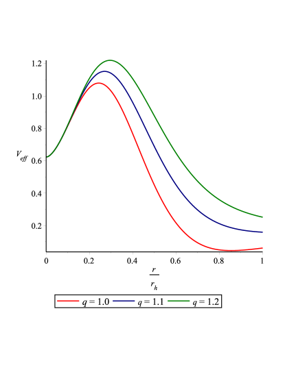
Figure 1: Effective potential for massless scalar field for $a=0.6$ (left) and $q=1.0$ (right) with $m=1$, $M=1$, $l=1$, $\alpha=0.01$ and $w=0.1$.

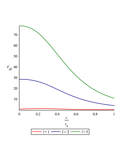
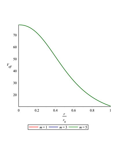
Figure 2: Effective potential for massless scalar field for $m=1$ (left) and $l=5$ (right) with $w=0.1$, $q=1$, $M=1$, $a=0.6$ and $\alpha=0.01$.

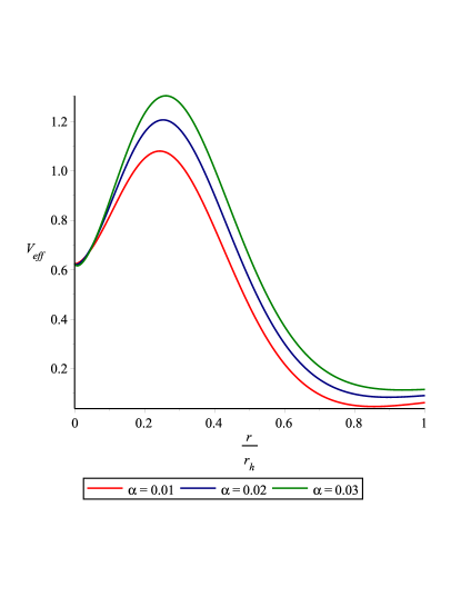
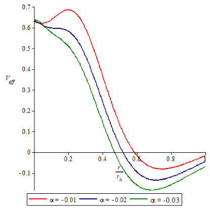
Figure 3: Effective potential for massless scalar field for $\alpha>0$ (left) and $\alpha<0$ (right) with $q=1.0$, $a=0.6$, $m=1$, $M=1$, $l=1$ and $w=0.1$.

3 Greybody Factor

This section provides the analytic solution of the greybody factor by using an appropriate technique on the radial equation of motion (5). We determine two asymptotic solutions for different regimes such as near and far-away from the BH horizon. To obtain the solution for the whole region, we compare these solutions smoothly in an intermediate regime.

We choose the following transformation to find the analytic solution for the near horizon region $r\sim r_{h}$

$$r\rightarrow Y=\frac{a^{2}+r^{2}-\frac{2Mr^{4}}{(r^{2}+q^{2})^{\frac{3}{2}}}+\alpha r\ln\frac{r}{|\alpha|}}{a^{2}+r^{2}+\alpha r\ln\frac{r}{|\alpha|}},$$ (6)

which gives

$$\frac{dY}{dr}=\frac{(1-Y)U(r_{h})}{r_{h}(r^{2}_{h}+q^{2})},$$

where

$$U(r_{h})=\frac{r^{2}_{h}(r^{2}_{h}+\alpha r_{h}-a^{2})-g^{2}\bigg{(}2(2a^{2}+r^{2}_{h})-\alpha r_{h}(1-3\ln\frac{r_{h}}{|\alpha|})\bigg{)}}{a^{2}+r^{2}_{h}+\alpha r_{h}\ln\frac{r_{h}}{|\alpha|}}.$$

Using these results in the radial equation (5), it follows that

$$Y(1-Y)\frac{d^{2}R_{wlm}}{dY^{2}}+(A-BY)\frac{dR_{wlm}}{dY}+\frac{1}{(1-Y)U^{2}}\bigg{[}\frac{\chi_{h}}{Y}-\lambda_{h}\bigg{]}R_{wlm}=0,$$ (7)

where

$$A = \frac{(r^{2}_{h}+q^{2})}{r^{2}_{h}U(r_{h})}\frac{d}{dr}\bigg{(}r^{3}_{h}YU(r_{h})\bigg{)},\quad B=\frac{5r^{2}}{U(r_{h})},$$

$$\chi_{h} = r^{2}_{h}(r^{2}_{h}+q^{2})^{2}\bigg{[}w^{2}(a^{2}+r^{2}_{h})^{2}+a^{2}m^{2}-2amw(a^{2}+r^{2}_{h}-\Omega)\bigg{]},$$

$$\lambda_{h} = \frac{r^{2}_{h}(r^{2}_{h}+q^{2})^{2}}{a^{2}+r^{2}_{h}+\alpha r_{h}\ln\frac{r_{h}}{|\alpha|}}(a^{2}w^{2}+\lambda^{m}_{l}).$$

We redefine the function in Eq.(7) as

$$R_{wlm}(Y)=Y^{\epsilon_{1}}(1-Y)^{\eta_{1}}\hat{F}(Y),$$

so that Eq.(7) takes the form

$$Y(1-Y)\frac{d^{2}\hat{F}(Y)}{dY^{2}}+\bigg{[}2\epsilon_{1}+A-(2\epsilon_{1}+2\eta_{1}+B)Y\bigg{]}\frac{d\hat{F}(Y)}{dY}+\bigg{[}\bigg{(}\epsilon^{2}_{1}-\epsilon_{1}$$

$$+A\epsilon_{1}+\frac{\chi^{\ast}_{h}}{U^{2}}\bigg{)}\frac{1}{Y}+\bigg{(}\eta^{2}_{1}-\eta_{1}-\eta_{1}A+\eta_{1}B+\frac{\chi_{h}}{U^{2}}-\frac{\lambda_{h}}{U^{2}}\bigg{)}\frac{1}{1-Y}\bigg{]}\hat{F}(Y)=0.$$

The power coefficients $\epsilon_{1}$ and $\eta_{1}$ can be calculated as

$$\epsilon^{2}_{1}-\epsilon_{1}+A\epsilon_{1}+\frac{\chi_{h}}{U^{2}}=0,$$

$$\eta^{2}_{1}-\eta_{1}-\eta_{1}A+\eta_{1}B+\frac{\chi_{h}}{U^{2}}-\frac{\lambda_{h}}{U^{2}}=0.$$

We finally obtain the hypergeometric (HG) type of differential equation of Eq.(5) as

$$Y(1-Y)\frac{d^{2}\hat{F}(Y)}{dY^{2}}+\bigg{[}\bar{c}_{1}-(1+\bar{a}_{1}+\bar{b}_{1})Y\bigg{]}\frac{d\hat{F}(Y)}{dY}-\bar{a}_{1}\bar{b}_{1}\hat{F}(Y)=0,$$

where

$$\bar{a}_{1}=\eta_{1}+\epsilon_{1}+B-1,\quad\bar{b}_{1}=\eta_{1}+\epsilon_{1},\quad\bar{c}_{1}=2\epsilon_{1}+A.$$

Its general solution for the near horizon (NH) is given as

$$(R_{wlm})_{NH}(Y) = \hat{A_{1}}Y^{\epsilon_{1}}(1-Y)^{\eta_{1}}\hat{F}(\bar{a}_{1},\bar{b}_{1},\bar{c}_{1};Y)+\hat{A_{2}}Y^{-\epsilon_{1}}(1-Y)^{\eta_{1}}$$ (8)

$$\times \hat{F}(1-\bar{c}_{1}+\bar{a}_{1},1-\bar{c}_{1}+\bar{b}_{1},-\bar{c}_{1}+2;Y),$$

where $\hat{A_{1}}$ and $\hat{A_{2}}$ are constants with

$$\epsilon^{\pm}_{1} = \frac{1}{2}\bigg{[}(1-A)\pm\sqrt{(1-A)^{2}-4\frac{\chi_{h}}{U^{2}}}\bigg{]},$$

$$\eta^{\pm}_{1} = \frac{1}{2}\bigg{[}(1+A-B)\pm\sqrt{(1+A-B)^{2}+4\bigg{(}\frac{\lambda_{h}}{U^{2}}-\frac{\chi_{h}}{U^{2}}\bigg{)}}\bigg{]}.$$

Applying the boundary conditions, i.e., no outgoing modes are observed near the BH horizon. We can choose either $\hat{A_{1}}=0$ or $\hat{A_{2}}=0$ which depends on the choice of $\epsilon_{1}$. It is found that the constants $\hat{A_{1}}$ and $\hat{A_{2}}$ remain the same for both values of $\epsilon_{1}$, so that we take $\epsilon_{1}^{+}=\epsilon_{1}^{-}$ by putting $\hat{A_{2}}=0$. The signs of $\eta_{1}$ can also be determined similarly by applying the convergence condition of the HG function which is valid for $\eta_{1}^{+}=\eta_{1}^{-}$. Thus the analytic solution for the NH takes the form

$$(R_{wlm})_{NH}(Y)=\hat{A_{1}}Y^{\epsilon_{1}}(1-Y)^{\eta_{1}}\hat{F}(\bar{a}_{1},\bar{b}_{1},\bar{c}_{1};Y).$$ (9)

Now we apply the above procedure for NH on the radial equation for far-away from BH horizon by replacing $\Omega(r)$ with $Z(r)$ as

$$Z(r)=1+\frac{a^{2}}{r^{2}}+\frac{\alpha}{r}\ln\frac{r}{|\alpha|}.$$ (10)

Consequently, the radial equation becomes

$$Z(1-Z)\frac{d^{2}R_{wlm}}{dZ^{2}}+(C-D^{\ast}Z)\frac{dR_{wlm}}{dZ}+\frac{1}{D^{2}(1-Z)}\bigg{[}\frac{\chi^{\ast}_{h}}{Z}-\lambda^{\ast}_{h}\bigg{]}R_{wlm}=0,$$

where

$$\chi^{\ast}_{h} = \frac{r^{2}Z^{2}}{\Omega^{2}}\bigg{[}w^{2}(a^{2}+r^{2})^{2}+a^{2}m^{2}-2amw(a^{2}+r^{2}-\Omega)\bigg{]},$$

$$\lambda^{\ast}_{h} = \frac{Zr^{2}}{\Omega}(a^{2}w^{2}+\lambda^{m}_{l}),\quad C=\frac{Z[\Omega(1-Z)D]^{{}^{\prime}}}{\Omega Z^{{}^{\prime}}D},\quad D^{\ast}=\frac{1}{D}.$$

Redefine the field in the above differential equation as

$$R_{wlm}(Z)=Z^{\epsilon_{2}}(1-Z)^{\eta_{2}}\hat{F(Z)},$$

we have

$$Z(1-Z)\frac{d^{2}\hat{F(Z)}}{dZ^{2}}+\bigg{[}2\epsilon_{2}+C-(2\epsilon_{2}+2\eta_{2}+D^{\ast})Z\bigg{]}\frac{d\hat{F(Z)}}{dZ}+\bigg{[}\bigg{(}\epsilon^{2}_{2}-\epsilon_{2}$$

$$+\epsilon_{2}C+\frac{\chi^{\ast}_{h}}{D^{2}}\bigg{)}\bigg{(}\eta_{2}^{2}-\eta_{2}-\eta_{2}C+\eta_{2}D^{\ast}+\frac{\chi^{\ast}_{h}}{D^{2}}-\frac{\lambda^{\ast}_{h}}{D^{2}}\bigg{)}\frac{1}{1-Z}\bigg{]}\hat{F(Z)}=0.$$

The power coefficients $\epsilon_{2}$ and $\eta_{2}$ can be found as

$$\epsilon^{2}_{2}-(1-C)\epsilon_{2}+\frac{\chi^{\ast}_{h}}{D^{2}}=0,$$

$$\eta^{2}_{2}-(1+C-D^{\ast})\eta_{2}+\frac{\chi^{\ast}_{h}}{D^{2}}-\frac{\lambda^{\ast}_{h}}{D^{2}}=0.$$

Hence, the above equation in terms of HG form with

$$\bar{a}_{2}=\epsilon_{2}+\eta_{2}+D^{\ast}-1,\quad\bar{b}_{2}=\epsilon_{2}+\eta_{2},\quad\bar{c}_{2}=2\epsilon_{2}+C,$$

becomes

$$Z(1-Z)\frac{d^{2}\hat{F(Z)}}{dZ^{2}}+\bigg{[}\bar{c}_{2}-(1+\bar{a}_{2}+\bar{b}_{2})\bigg{]}\frac{d\hat{F(Z)}}{dZ}-\bar{a}_{2}\bar{b}_{2}\hat{F(Z)}=0.$$

Its general solution is

$$(R_{wlm})_{f}(Z) = \hat{B_{1}}Z^{\epsilon_{2}}(1-Z)^{\eta_{2}}\hat{F}(\bar{a}_{2},\bar{b}_{2},\bar{c}_{2};Z)+\hat{B_{2}}Z^{-\epsilon_{2}}(-Z+1)^{\eta_{2}}$$ (11)

$$\times \hat{F}(1-\bar{c}_{2}+\bar{a}_{2},1-\bar{c}_{2}+\bar{b}_{2},-\bar{c}_{2}+2;Z),$$

with

$$\epsilon_{2} = \frac{1}{2}\bigg{[}(1-C)\pm\sqrt{(1-C)^{2}-4\frac{\chi^{\ast}_{h}}{D^{2}}}\bigg{]},$$

$$\eta_{2} = \frac{1}{2}\bigg{[}(1+C-D^{\ast})\pm\sqrt{(1+C-D^{\ast})^{2}-4\bigg{(}\frac{\chi^{\ast}_{h}}{D^{2}}-\frac{\lambda^{\ast}_{h}}{D^{2}}\bigg{)}}\bigg{]},$$

where $\hat{B_{1}}$ and $\hat{B_{2}}$ are arbitrary constants. Similar to NH, we choose the HG convergence condition to compare the solutions with the same choices of $\epsilon_{2}^{+}=\epsilon_{2}^{-}$ and $\eta_{2}^{+}=\eta_{2}^{-}$.

4 Matching to an Intermediate Regime

This section is devoted to matching the obtained solutions (NH and far-away) efficiently in the intermediate region for all values of $r$. In this scenario, we expand the solution by changing the HG function argument $Y$ to $1-Y$ in Eq.(9) as

$$(R_{wlm})_{NH}(Y) = (-Y+1)^{\eta_{1}}\bigg{[}\frac{\Gamma(-\bar{a}_{1}-\bar{b}_{1}+\bar{c}_{1})\Gamma(\bar{c}_{1})}{\Gamma(-\bar{a}_{1}+\bar{c}_{1})\Gamma(-\bar{b}_{1}+\bar{c}_{1})}\hat{F}(\bar{a}_{1},\bar{b}_{1},\bar{c}_{1};1-Y)$$

$$+ (1-Y)^{-\bar{a}_{1}-\bar{b}_{1}+\bar{c}_{1}}\frac{\Gamma(\bar{c}_{1})\Gamma(-\bar{c}_{1}+\bar{b}_{1}+\bar{a}_{1})}{\Gamma(\bar{b}_{1})\Gamma(\bar{a}_{1})}$$

$$\times \hat{F}(+\bar{c}_{1}-\bar{a}_{1},+\bar{c}_{1}-\bar{b}_{1},1-\bar{a}_{1}-\bar{b}_{1}+\bar{c}_{1};1-Y)\bigg{]}\hat{A_{1}}Y^{\epsilon_{1}}.$$

Using Eq.(2) in (6), it follows that

$$1-Y=\frac{2Mr^{4}}{(r^{2}+q^{2})^{\frac{3}{2}}(r^{2}+a^{2}+\alpha r\ln\frac{r}{|\alpha|})}.$$

The stretched NH for $Y\rightarrow 1$ and limiting value of $r\gg r_{h}$ yield

$$(1-Y)^{\eta_{1}}\simeq\bigg{[}\frac{r_{h}(q_{\ast}^{2}+1)^{\frac{3}{2}}(a_{\ast}^{2}+1+\alpha_{\ast}\ln\frac{r_{h}}{|\alpha|})}{r}\bigg{]}^{\eta_{1}}$$

$$\simeq\bigg{[}\frac{r_{h}(q_{\ast}^{2}+1)^{\frac{3}{2}}(1+a_{\ast}^{2}+\alpha_{\ast}\ln\frac{r_{h}}{|\alpha|})}{r}\bigg{]}^{-l},$$

and

$$(1-Y)^{\eta_{1}-\bar{a}_{1}-\bar{b}_{1}+\bar{c}_{1}} \simeq \bigg{[}\frac{r_{h}(1_{\ast}^{2}+1)^{\frac{3}{2}}(1+a_{\ast}^{2}+\alpha_{\ast}\ln\frac{r_{h}}{|\alpha|})}{r}\bigg{]}^{-\eta_{1}+A-B+1},$$

$$\simeq \bigg{[}\frac{r_{h}(q_{\ast}^{2}+1)^{\frac{3}{2}}(1+a_{\ast}^{2}+\alpha_{\ast}\ln\frac{r_{h}}{|\alpha|})}{r}\bigg{]}^{1+l},$$

where $a_{\ast}=\frac{a}{r}$, $q_{\ast}=\frac{q}{r}$ and $\alpha_{\ast}=\frac{\alpha}{r}$. We would like to mention here that all the above constraints are valid for smaller values of charge and rotation parameter. In an intermediate zone, the NH solution can be expressed as

$$(R_{wlm})_{NH}(Y)=\tilde{A_{1}}\bigg{(}\frac{r}{r_{h}}\bigg{)}^{-l}+\tilde{A_{2}}\bigg{(}\frac{r}{r_{h}}\bigg{)}^{-(1+l)},$$ (12)

with

$$\tilde{A_{1}} = \hat{A_{1}}\bigg{[}(1+q_{\ast}^{2})^{\frac{3}{2}}(1+a_{\ast}^{2}+\alpha_{\ast}\ln\frac{r_{h}}{|\alpha|})\bigg{]}^{-l}\frac{\Gamma(\bar{c}_{1})\Gamma(-\bar{a}_{1}-\bar{b}_{1}+\bar{c}_{1})}{\Gamma(+\bar{c}_{1}-\bar{b}_{1})\Gamma(+\bar{c}_{1}-\bar{a}_{1})},$$

$$\tilde{A_{2}} = \bigg{[}(q_{\ast}^{2}+1)^{\frac{3}{2}}(1+a_{\ast}^{2}+\alpha_{\ast}\ln\frac{r_{h}}{|\alpha|})\bigg{]}^{1+l}\frac{\Gamma(\bar{a}_{1}+\bar{b}_{1}-\bar{c}_{1})\Gamma(\bar{c}_{1})}{\Gamma(\bar{a}_{1})\Gamma(\bar{b}_{1})}.$$

Now, we find the solution far away from the BH event horizon and stretch the HG function arguments by changing $Z$ with $1-Z$ with $Z(r_{f})\rightarrow 0$. Hence, Eq.(11) reduces to

$$(1-Z)^{\eta_{2}}\simeq\bigg{(}\frac{\ln\frac{r}{|\alpha|}}{\ln\frac{r_{f}}{|\alpha|}}\bigg{)}^{-l}\bigg{(}\frac{r}{r_{f}}\bigg{)}^{l},$$

and

$$(1-Z)^{\eta_{2}+\bar{c}_{2}-\bar{a}_{2}-\bar{b}_{2}}\simeq\bigg{(}\frac{r}{r_{f}}\bigg{)}^{-(1+l)}\bigg{(}\frac{\ln\frac{r}{|\alpha|}}{\ln\frac{r_{f}}{|\alpha|}}\bigg{)}^{1+l}.$$

We restrict the parameters $a$ and $q$ to smaller values for the far-field horizon and the solution of Eq.(11) yields

$$(R_{wlm})_{f}(Z)=\bigg{(}\tilde{H_{1}}\tilde{B_{1}}+\tilde{H_{2}}\tilde{B_{2}}\bigg{)}\bigg{(}\frac{r}{r_{f}}\bigg{)}^{l}+\bigg{(}\tilde{H_{3}}\tilde{B_{1}}+\tilde{H_{4}}\tilde{B_{2}}\bigg{)}\bigg{(}\frac{r}{r_{f}}\bigg{)}^{-(1+l)},$$ (13)

where

$$\tilde{H_{1}} = \frac{\Gamma(\bar{c}_{2})\Gamma(\bar{c}_{2}-\bar{a}_{2}-\bar{b}_{2})}{\Gamma(\bar{c}_{2}-\bar{a}_{2})\Gamma(\bar{c}_{2}-\bar{b}_{2})}\bigg{(}\frac{\ln\frac{r}{|\alpha|}}{\ln\frac{r_{f}}{|\alpha|}}\bigg{)}^{-l},$$

$$\tilde{H_{2}} = \frac{\Gamma(2-\bar{c}_{2})\Gamma(-\bar{a}_{2}-\bar{b}_{2}+\bar{c}_{2})}{\Gamma(1-\bar{a}_{2})\Gamma(1-\bar{b}_{2})}\bigg{(}\frac{\ln\frac{r}{|\alpha|}}{\ln\frac{r_{f}}{|\alpha|}}\bigg{)}^{-l},$$

$$\tilde{H_{3}} = \frac{\Gamma(\bar{c}_{2})\Gamma(-\bar{c}_{2}+\bar{b}_{2}+\bar{a}_{2})}{\Gamma(\bar{b}_{2})\Gamma(\bar{a}_{2})}\bigg{(}\frac{\ln\frac{r}{|\alpha|}}{\ln\frac{r_{f}}{|\alpha|}}\bigg{)}^{1+l},$$

$$\tilde{H_{4}} = \frac{\Gamma(2-\bar{c}_{2})\Gamma(-\bar{c}_{2}+\bar{a}_{2}+\bar{b}_{2})}{\Gamma(\bar{a}_{2}-\bar{c}_{2}+1)\Gamma(\bar{b}_{2}-\bar{c}_{2}+1)}\bigg{(}\frac{\ln\frac{r}{|\alpha|}}{\ln\frac{r_{f}}{|\alpha|}}\bigg{)}^{1+l}.$$

We compare both the asymptotic solutions with the similar powers of $l$ and $1+l$ as

$$\tilde{A_{1}}=\tilde{H_{1}}\tilde{B_{1}}+\tilde{H_{2}}\tilde{B_{2}},\quad\tilde{A_{2}}=\tilde{H_{3}}\tilde{B_{1}}+\tilde{H_{4}}\tilde{B_{2}}.$$

The integration constants $\tilde{B_{1}}$ and $\tilde{B_{2}}$ are found to be

$$\tilde{B_{2}}=\frac{\tilde{A_{1}}\tilde{H_{3}}-\tilde{A_{2}}\tilde{H_{1}}}{\tilde{H_{2}}\tilde{H_{3}}-\tilde{H_{1}}\tilde{H_{4}}},\quad\tilde{B_{1}}=\frac{\tilde{A_{1}}\tilde{H_{4}}-\tilde{A_{2}}\tilde{H_{2}}}{\tilde{H_{1}}\tilde{H_{4}}-\tilde{H_{2}}\tilde{H_{3}}}.$$

In order to calculate the emission rate of massless scalar field, we have the expression of greybody factor as [41]

$$|A_{l,m}|^{2}=1-\bigg{|}\frac{\tilde{B_{2}}}{\tilde{B_{1}}}\bigg{|}^{2}=1-\bigg{|}\frac{\tilde{A_{2}}\tilde{H_{1}}-\tilde{A_{1}}\tilde{H_{3}}}{\tilde{A_{1}}\tilde{H_{4}}-\tilde{A_{2}}\tilde{H_{2}}}\bigg{|}^{2}.$$

This is a combination of greybody factor (absorption probability) and emission rate of massless scalar field derived from the rotating regular Bardeen BH. It is noted that the waves passing through far-away from the horizon will face the barrier which works as a filter to either move forward or reflect. It is a relative relation between frequency and effective potential. The frequency of the wave must be larger than the effective potential to cross the barrier. If the potential exceeds the wave frequency, some portions are reflected while some may cross the barrier and consequently, the greybody factor displays a negative trend.

We sketch the above expression for different parameters to discuss viability of the greybody factor numerically. The effects of parameters $a$ and $l$ are analyzed on the profile of the greybody factor. Figure 4 indicates that the absorption rate of scalar field increases for higher values of the rotation parameter as well as angular momentum. Figure 5 shows the influence of $q$ for the absorption rate of the massless scalar field. It is found that BH absorbs partial waves with the increasing values of magnetic charge which increases the greybody factor and reduces the emission rate of the scalar field. The impact of PFDM parameter $\alpha$ on the greybody factor is shown in Figure 6. It is noted that increasing the value of $\alpha$ yields a high rate of absorption probability of initial waves and raises the greybody factor.

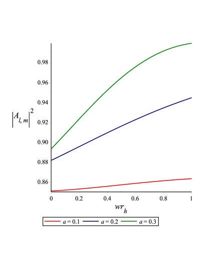
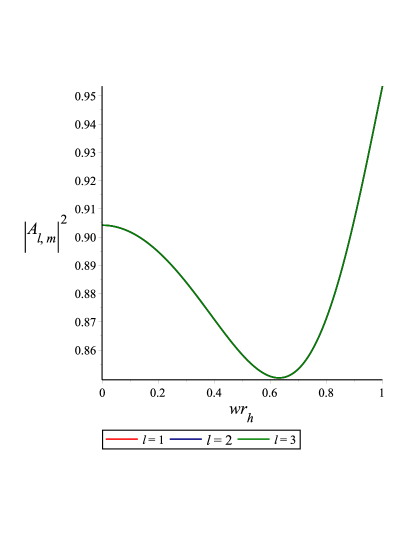
Figure 4: Greybody factor for massless scalar field for $l=1$ (left) and $a=0.1$ (right) with $r=0.5$, $m=1$, $M=1$, $q=0.1$ and $\alpha=0.01$.

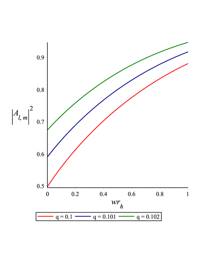
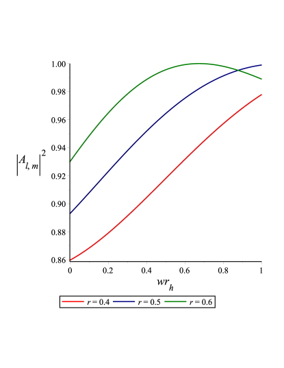
Figure 5: Greybody factor for massless scalar field for $r=0.4$ (left) and $q=0.1$ (right) with $a=0.1$, $l=1$, $m=1$, $M=1$, $\alpha=0.01$.

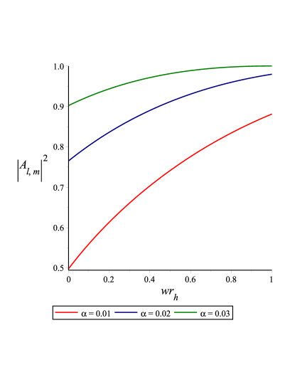
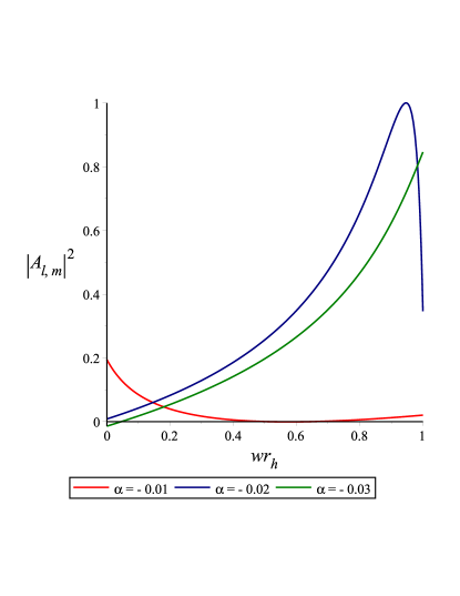
Figure 6: Greybody factor for massless scalar field for $\alpha>0$ (left) and $\alpha<0$ (right) with $a=0.1$, $r=0.1$, $l=1$, $m=1$, $M=1$ and $q=0.1$.

The total amount of massless scalar particles discharged per unit time and frequency from a BH (particle flux) can be found as

$$\frac{d^{2}\widetilde{P}}{dtdw}=\sum_{l,m}|A_{l,m}|^{2}\frac{1}{2\pi e^{-1+\frac{\kappa}{T_{H}}}}=\sum_{l,m}\bigg{(}1-\bigg{|}\frac{\tilde{A_{1}}\tilde{H_{4}}-\tilde{A_{2}}\tilde{H_{2}}}{\tilde{A_{1}}\tilde{H_{3}}-\tilde{A_{2}}\tilde{H_{1}}}\bigg{|}^{2}\bigg{)}\frac{1}{2\pi e^{-1+\frac{\kappa}{T_{H}}}},$$

and

$$\frac{d^{2}\widetilde{N}}{dtdw}=\sum_{l,m}|A_{l,m}|^{2}\frac{w}{2\pi e^{-1+\frac{\kappa}{T_{H}}}}=\sum_{l,m}\bigg{(}1-\bigg{|}\frac{\tilde{A_{1}}\tilde{H_{4}}-\tilde{A_{2}}\tilde{H_{2}}}{\tilde{A_{1}}\tilde{H_{3}}-\tilde{A_{2}}\tilde{H_{1}}}\bigg{|}^{2}\bigg{)}\frac{w}{2\pi e^{-1+\frac{\kappa}{T_{H}}}}.$$

Also, we can have

$$\kappa=-\frac{am}{a^{2}+r^{2}}+w,\quad T_{H}=\frac{1-\frac{a^{2}}{r^{2}}}{4\pi r_{h}(1+\frac{a^{2}}{r^{2}})}.$$

The differential equation for the emission rate of angular momentum can also be written in a similar way. The absorption cross-section of each partial wave can be calculated as

$$\sigma=\sum_{l,m}\frac{\pi}{w^{2}}|A_{l,m}|^{2}=\sum_{l,m}\frac{\pi}{w^{2}}\bigg{(}1-\bigg{|}\frac{\tilde{A_{1}}\tilde{H_{4}}-\tilde{A_{2}}\tilde{H_{2}}}{\tilde{A_{1}}\tilde{H_{3}}-\tilde{A_{2}}\tilde{H_{1}}}\bigg{|}^{2}\bigg{)}.$$

5 Concluding Remarks

In this paper, we have formulated the analytic model of the greybody factor for rotating Bardeen BH surrounded by PFDM. We have first calculated the effective potential using the Klein-Gordon equation and examined the graphical analysis for different parameters. The Klein-Gordon equation gives spheroidal and radial equations. The radial equation is then used to determine two asymptotic solutions near and far-away from to BH horizon. These two solutions are matched smoothly in an intermediate regime to find the general expression of the greybody factor in low rotation and low energy regimes. We have also evaluated the absorption cross-section and emission rate for a massless scalar field.

We have analyzed the effective potential and greybody factor for different values of physical parameters in a low energy regime. It is found that the barrier’s height and absorption rate increase with large values of the rotation parameter. This reduces the emission rate of radiations and raises its probability of absorption. We have seen that the greybody factor increases with the effects of angular momentum as well as magnetic charge. We have found that BH does not emit radiations through the barrier but absorb rapidly which raises the greybody factor. It is found that higher modes of PFDM parameter yields a high rate of absorption probability. We note that rotating and non-rotating regular BHs evaporate rapidly as compared to other BHs as they emit thermal flux of quantum level particles. Hence the rotating Bardeen BH surrounded by PFDM would not squeeze and disappear faster as it has the ability to absorb massless scalar field particles.

It is interesting to mention here that the absorption rate of scalar field remains the same for both rotating Bardeen as well as Kerr BHs [42]. It is known that PFDM parameter for non-rotating Bardeen BH increases the emission rate but decreases the absorption rate of scalar field [37]. However, we have found the opposite behavior for the rotating case where the PFDM parameter decreases the emission rate but increases the absorption rate of scalar field. We conclude that the the PFDM parameter of rotating Bardeen BH with PFDM increases the greybody factor. When the rotation parameter vanishes, our results reduce to the results given in [37]. It is worthwhile to mention here that all our results reduce to the corresponding results of Schwarzschild BH when $a=0=\alpha=q$.

References

• [1] Bardeen, J.M.: Proceedings of GR5 (Tiflis, USSR, 1968)174.
• [2] Hayward, S.: Phys. Rev. Lett. 96(2006)031103.
• [3] Bambi, C. and Modesto, L.: Phys. Lett. B 721(2013)329.
• [4] Kiselev, V.V.: Class. Quantum Grav. 20(2003)1187.
• [5] Chen, S. and Jing, J.: Class. Quantum Grav. 22(2005)4651; ibid. 23(2006)6141; Gen. Relativ. Gravit. 39(2007)1003.
• [6] Xu, Z., Hou, X. and Wang, J.: Class. and Quantum Grav. 35(2018)115003.
• [7] Xu, Z., et al.: Eur. Phys. J. C 78(2018)513.
• [8] Hou, X., et al.: Advance High Energy Phys. 2019(2019)2434390.
• [9] Hawking, S.W.: Commun. Math. Phys. 43(1975)199.
• [10] Gubserv, S.S. and Klebanov, I.R.: Phys. Rev. Lett. 77(1996)4491.
• [11] Maldacena, J.M. and Strominger, A.: Phys. Rev. D 55(1997)861.
• [12] Klebanov, I.R. and Mathur, S.D.: Nucl. Phys. B 500(1997)115.
• [13] Kim, W.T. and Oh, J.J.: Phys. Lett. B 461(1999)189.
• [14] Creek, S. et al.: Phys. Lett. B 656(2007)102.
• [15] Boonserm, P. et al.: J. Math. Phys. 55(2014)112502.
• [16] Jorge, R., de Oliveira, E.S. and Rocha, J.V.: Class. Quantum Grav. 32(2015)065008.
• [17] Toshmatov, B. et al.: Phys. Rev. D 91(2015)083008.
• [18] Ahmad, J. and Saifullah, K.: Eur. Phys. J. C 77(2017)885.
• [19] Hyun, Y.H., Kimb, Y. and Park, S.C.: J. High Energy Phys. 6(2019)41.
• [20] Dey, S. and Chakrabarti, S.: Eur. Phys. J. C 79(2019)504.
• [21] Ida, D., Oda, k. and Park, S.C.: Phys. Rev. D 67(2003)064025.
• [22] Chen, S., Wang, B. and Su, R.: Phys. Rev. D 77(2008)124011.
• [23] Crispino, L.C.B. et al.: Phys. Rev. D 87(2013)104034.
• [24] Kanti, P., Pappas, T. and Pappas, N.: Phys. Rev. D 90(2014)124077.
• [25] Ahmad, J. and Saifullah, K.: Eur. Phys. J. C 78(2018)316.
• [26] Sharif, M. and Ama-Tul-Mughani, Q.: Eur. Phys. J. Plus 134(2019)616; Phys. Dark Universe 27(2020)100436.
• [27] Sakalli, I.: Phys. Rev. D 94(2016)084040.
• [28] Sakalli, I. and Aslan, O.A.: Astropart. Phys. 74(2016)73.
• [29] Kanzi, S. and Sakalli, I. Nuclear Phys. B 946(2019)114703.
• [30] Gursel, H. and Sakalli, I.: Eur. Phys. J. C 80(2020)34.
• [31] Jusufi, K. et al., Phys. Rev. D 102(2020)064020.
• [32] Rahaman, F., et al.: Phys. Lett. B 694(2010)10.
• [33] Hou, X., Xu, Z. and Wang, J.: Eur. Phys. J. 12(2018)040.
• [34] Jamil, M., et al.: Phys. Rev. D 100(2019)044012.
• [35] Hendi, S.H., et al.: Eur. Phys. J. C 80(2020)296.
• [36] Das, A., et al.: Class. Quantum Grav. 38(2021)065015.
• [37] Ama-Tul-Mughani, Q., Salam, W. and Saleem, R.: Astroparticle Phys. 132(2021)102623.
• [38] Zhang, H.X. et al.: Chin. Phys. C 45(2021)055103.
• [39] Flammer, C.: Spheroidal Wave Functions (Stanford University Press, 1957).
• [40] Berti, E., Cardoso, V. and Casals, M.: Phys. Rev. D 73(2006)024013; ibid. 109902.
• [41] Sanchez, N.: Phys. Rev. D 18(1978)1030.
• [42] Macedo, C.F., et al.: Phys. Rev. D 88(2013)064033.