Efficient Neural Radiance Fields for Interactive Free-viewpoint Video

Abstract.

This paper aims to tackle the challenge of efficiently producing interactive free-viewpoint videos. Some recent works equip neural radiance fields with image encoders, enabling them to generalize across scenes. When processing dynamic scenes, they can simply treat each video frame as an individual scene and perform novel view synthesis to generate free-viewpoint videos. However, their rendering process is slow and cannot support interactive applications. A major factor is that they sample lots of points in empty space when inferring radiance fields. We propose a novel scene representation, called ENeRF, for the fast creation of interactive free-viewpoint videos. Specifically, given multi-view images at one frame, we first build the cascade cost volume to predict the coarse geometry of the scene. The coarse geometry allows us to sample few points near the scene surface, thereby significantly improving the rendering speed. This process is fully differentiable, enabling us to jointly learn the depth prediction and radiance field networks from RGB images. Experiments on multiple benchmarks show that our approach exhibits competitive performance while being at least 60 times faster than previous generalizable radiance field methods.

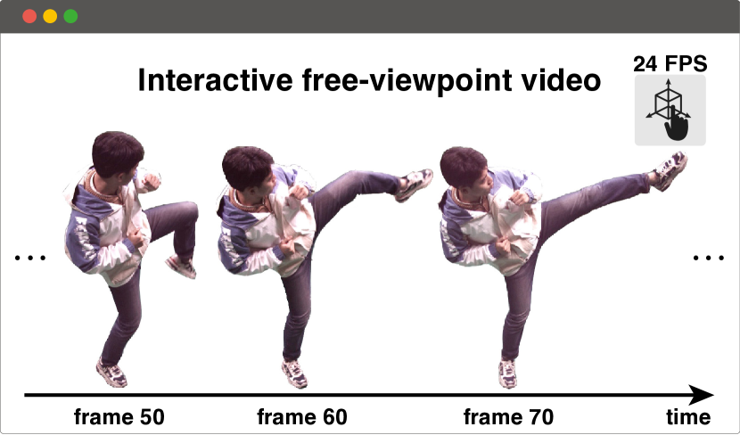
Figure 1. The proposed method achieves photorealistic view synthesis for dynamic scenes at interactive frame rates. Please refer to our video for the real-time demos that render free-viewpoint videos of dynamic scenes.

1. Introduction

Free-viewpoint videos have a variety of applications such as virtual tourism, immersive telepresence, and movie production. These applications generally require us to accomplish two things. First, given multi-view videos, we need to quickly generate the free-viewpoint video, which is essential for immersive telepresence. Second, rendering novel views of target scenes should be fast, which is important for user experience. Neural radiance field (NeRF) (Mildenhall et al., 2020) represents scenes as density and radiance fields, enabling it to achieve photorealistic novel view synthesis. (Pumarola et al., 2021; Park et al., 2021a) leverage deformation fields to extend NeRF to dynamic scenes and thus can produce free-viewpoint videos. However, these methods generally require a long training process for each new scene. Moreover, their rendering speed is slow.

Recently, (Yu et al., 2021a; Garbin et al., 2021) propose to cache radiance fields into highly efficient data structures, which significantly improves the rendering speed. To handle dynamic scenes, FastNeRF (Garbin et al., 2021) augments the cached scene with deformation fields that transform the world-space points to the space of the cached scene. Although it can render free-viewpoint videos in real-time, there are two problems. First, the deformation fields are difficult to be recovered from videos when there exist complex scene motions, as discussed in (Peng et al., 2021a). Second, it still needs a lengthy optimization process, making it impossible to quickly produce free-viewpoint videos from new data.

Another line of works (Yu et al., 2021b; Wang et al., 2021b) train networks to predict radiance fields from multi-view images and can generalize to unseen scenes. These methods overcome the two problems of FastNeRF (Garbin et al., 2021). First, when processing dynamic scenes, they are able to simply treat every frame as an individual scene and perform novel view synthesis, instead of recovering temporal motions like (Pumarola et al., 2021; Garbin et al., 2021). Second, thanks to the pretraining, they can be quickly fine-tuned to produce photorealistic rendering results on new scenes. However, their rendering speed is slow, as they require many forward passes through a neural network for rendering a pixel.

In this paper, we propose a novel rendering approach, called ENeRF, for efficiently generating interactive free-viewpoint videos. Our innovation lies in introducing a learned depth-guided sampling strategy that greatly speeds up the rendering of generalizable radiance field methods. Specifically, for the target view, we construct the cascade cost volume, which is used to predict a depth probability distribution. The depth probability distribution gives an interval in which the surface may be located. With the depth interval, we only need to sample few 3D points along the ray and thus improve the rendering speed of previous methods (Wang et al., 2021b; Chen et al., 2021). Similar to (Chen et al., 2021), we predict radiance fields using the cost volume feature, which makes our method generalize well to new scenes. Moreover, the whole pipeline is fully differentiable, so the depth-guided sampling strategy can be jointly learned with NeRF from only multi-view RGB images.

We evaluate our approach on the DTU (Jensen et al., 2014), Real Forward-facing (Mildenhall et al., 2020, 2019), NeRF Synthetic (Mildenhall et al., 2020), DynamicCap (Habermann et al., 2021) and ZJU-MoCap (Peng et al., 2021b) datasets, which are widely-used benchmark datasets for novel view synthesis. Our approach makes significant rendering acceleration while achieving competitive results with baselines across all datasets. Specifically, our approach runs at least 60 times faster than previous generalizable radiance field methods (Yu et al., 2021b; Wang et al., 2021b; Chen et al., 2021). We also show that our approach can produce reasonable depth maps by supervising the networks with only images.

In summary, this work has the following contributions: 1) We propose a novel approach that utilizes a learned depth-guided sampling strategy to improve the rendering efficiency of generalizable radiance field methods. 2) We show that the depth-guided sampling can be jointly learned with NeRF from only RGB images. 3) We demonstrate that our approach runs significantly faster than previous methods while being competitive on the rendering quality on several view synthesis benchmarks. 4) We demonstrate the capability of our method to synthesize novel views of human performers in real-time. Our code is available at https://zju3dv.github.io/enerf.

2. Related work

Novel view synthesis.

Some methods achieves the free-viewpoint rendering based on the light field interpolation (Gortler et al., 1996; Levoy and Hanrahan, 1996; Davis et al., 2012) or image-based rendering (Zitnick et al., 2004; Chaurasia et al., 2013; Flynn et al., 2016; Kalantari et al., 2016; Penner and Zhang, 2017; Riegler and Koltun, 2020). Recently, neural representations (Sitzmann et al., 2019; Liu et al., 2019b; Li et al., 2020; Lombardi et al., 2019; Shih et al., 2020; Liu et al., 2019a; Jiang et al., 2020; Wizadwongsa et al., 2021) are widely used for novel view synthesis, which can be optimized from input images and achieve photorealistic rendering results. Neural radiance field (NeRF) (Mildenhall et al., 2020) represents scenes as continuous color and density fields and yields impressive rendering results. There are some works (Yu et al., 2021b; Trevithick and Yang, 2021; Wang et al., 2021b; Chen et al., 2021; Liu et al., 2021b; Johari et al., 2022) that attempt to improve NeRF on the training speed. They use 2D CNNs to process input images and decode multi-view features to target radiance fields. By pre-training networks, they can be quickly fine-tuned to produce high-quality rendering results on new scenes. More recently, (Yu et al., 2022; Müller et al., 2022; Sun et al., 2021; Chen et al., 2022; Sun et al., 2022) develop hybrid or explicit structures based on NeRF and achieve super-fast convergence for radiance fields reconstruction. Another line of works (Liu et al., 2020; Yu et al., 2021a; Reiser et al., 2021; Garbin et al., 2021; Hedman et al., 2021) aim to accelerate the rendering speed of NeRF. By caching neural radiance fields, (Garbin et al., 2021) can synthesize photorealistic images in real time. Some methods (Fang et al., 2021; Arandjelović and Zisserman, 2021; Barron et al., 2021; Piala and Clark, 2021; Neff et al., 2021) improve the sampling strategy of NeRF to accelerate the rendering. DONeRF (Neff et al., 2021) uses the depth-guided sampling for NeRF. However, it needs depth supervision and requires per-scene optimization. There exists some methods (Deng et al., 2022; Roessle et al., 2022; Rematas et al., 2022; Wei et al., 2021) exploring depth supervision to facilitate the reconstruction of neural radiance fields. In the field of 3D generation, (Gu et al., 2022) accelerates the rendering of 3D GAN with an upsampler to upsample a low-resolution feature map.  (Chan et al., 2022) enables real-time rendering of 3D GAN using a tri-plane representation. The above works mainly focus on view synthesis of static scenes.

Figure 2. Illustration of the proposed approach. Given multi-view images of a static scene or a dynamic scene at one frame, we first construct the cascade cost volume, which is processed to output the 3D feature volume and the coarse scene geometry (represented by depth and confidence maps). The estimated geometry guides us to sample around the surface, which significantly accelerates the volume rendering process. Also, the 3D feature volume provides rich geometry-aware information for generalizable radiance fields construction. All network components are trained end-to-end using only RGB images.

View synthesis of dynamic scenes.

Some methods (Li et al., 2021; Xian et al., 2021; Li et al., 2022) treat dynamic scenes as 4D domain and add the time dimension to the input spatial coordinate to implement the space-time radiance fields. To produce free-viewpoint videos from monocular videos, (Park et al., 2021a; Pumarola et al., 2021; Park et al., 2021b) propose to aggregate the temporal information of input videos. DNeRF (Pumarola et al., 2021) augments NeRF with deformation fields that establish correspondences between the canonical scene and the scenes at different time instants. (Zhang et al., 2021) develop a layered neural representation based on DNeRF, thereby better handling dynamic scenes containing multiple persons and static background. Although these methods achieve impressive rendering results on dynamic scenes, they typically have a slow rendering speed. FastNeRF (Garbin et al., 2021) caches the canonical NeRF and uses a small MLP to predict the deformation fields, which improves the rendering speed. However, it can only achieve the real-time rendering on $300\times 300$ images. Moreover, the deformation fields are difficult to estimated from videos on complex dynamic scenes, as discussed in Peng et al. (2021a). More recently, (Zhang et al., 2022; Wang et al., 2022) introduce 4D volumetric representations, which achieves efficient generation of free-viewpoint videos. They generally handle videos with short frames. In the field of human rendering, (Peng et al., 2021b, a; Weng et al., 2022; Lombardi et al., 2021; Liu et al., 2021a) utilize human priors to model human motions and thus accomplish the free-viewpoint rendering of dynamic human performers. Generalizable radiance fields (Wang et al., 2021b; Yu et al., 2021b) can be used to render dynamic scenes by individually processing the scene at each time, which overcomes the problem of recovering temporal motions. However, its rendering speed is slow.

Multi-view stereo methods.

The cost volume has been widely used for depth estimation in multi-view stereo (MVS) methods. MVSNet (Yao et al., 2018) proposes to build the 3D cost volume from 2D image features and regularizes it with a 3D CNN. This design enables end-to-end training of the network with ground truth depth and achieves impressive results. However, memory consumption of MVSNet is huge. To overcome this problem, following works improve it with recurrent plane sweeping (Yao et al., 2019) or coarse-to-fine architectures (Chen et al., 2019; Yu and Gao, 2020; Gu et al., 2020; Cheng et al., 2020). In the field of novel view synthesis, (Chen et al., 2021; Chibane et al., 2021) attempt to combine MVS methods with neural radiance field methods. They (2021) aim to facilitate the construction of the radiance fields leveraging stereo features. In contrast, our method focuses on accelerating the rendering process with explicit geometry. Another line of works (Oechsle et al., 2021; Yariv et al., 2021; Wang et al., 2021a) combine multi-view stereo and neural radiance fields to facilitate geometry reconstruction.

3. Method

Given multi-view images, our task is to generate images of novel views at interactive frame rates. As shown in Figure 2, to generate a novel view from multi-view images, we first extract multi-scale feature maps from input images, which are used to estimate coarse scene geometry and neural radiance fields (Sec. 3.1). Given extracted feature maps, we construct the cascade cost volume to obtain the 3D feature volume and the coarse scene geometry (Sec. 3.2). The feature volume provides geometry-aware information for radiance fields construction, and the estimated coarse geometry allows us to sample around the surface, which significantly accelerates the rendering process (Sec. 3.3). All networks are trained end-to-end with the view synthesis loss using only RGB images (Sec. 3.4).

3.1. Multi-scale image feature extraction

To build the cascade cost volume, we first extract multi-scale image features from input views $\{I_{i}\}_{i=1}^{N}$ using a 2D UNet. As shown in Figure 2, we first feed an input image $I_{i}\in\mathbb{R}^{H\times W\times 3}$ into the encoder to obtain low-resolution feature maps $F_{i,1}\in\mathbb{R}^{H/4\times W/4\times 32}$. Then we use two deconvolution layers to upsample the feature maps and obtain the other two-stage feature maps $F_{i,2}\in\mathbb{R}^{H/2\times W/2\times 16}$ and $F_{i,3}\in\mathbb{R}^{H\times W\times 8}$ . $F_{i,1}$ and $F_{i,2}$ are used to construct cost volumes, and $F_{i,3}$ is used to reconstruct neural radiance fields.

3.2. Coarse-to-fine depth prediction

To efficiently obtain the coarse scene geometry (represented by a high-resolution depth map) from multi-view images, we construct the cascade cost volume under the novel view frustum to predict the depth for the novel view. Specifically, we first construct a coarse-level low-resolution cost volume and recover a low-resolution depth map from this cost volume. Then we construct a fine-level high-resolution cost volume utilizing the depth map estimated in the last step. The fine-level cost volume is processed to produce a high-resolution depth map and a 3D feature volume.

Coarse-level cost volume construction.

Given initial scene depth range, we first sample a set of depth planes $\{\mathbf{L}_{i}|i=1,...,D\}$. Following learning-based MVS methods (Yao et al., 2018), we construct the cost volume by warping image features $F_{i,1}$ into $D$ sweeping planes. Given camera intrinsic, rotation and translation $[\mathbf{K}_{i},\mathbf{R}_{i},\mathbf{t}_{i}]$ of input view $I_{i}$ and $[\mathbf{K}_{t},\mathbf{R}_{t},\mathbf{t}_{t}]$ of target view, the homography warping is defined as:

(1) $$\mathbf{H}_{i}(z)=\mathbf{K}_{i}\mathbf{R}_{i}\Big{(}\mathbf{I}+\frac{(\mathbf{R}_{i}^{-1}\mathbf{t}_{i}-\mathbf{R}_{t}^{-1}\mathbf{t}_{t})\mathbf{a}^{T}\mathbf{R}_{t}}{z}\Big{)}\mathbf{R}_{t}^{-1}\mathbf{K}_{t}^{-1},$$

where $\mathbf{a}$ denotes the principal axis of the target view camera, $\mathbf{I}$ is the identity matrix and $\mathbf{H}_{i}(z)$ warps a pixel $(u,v)$ in the target view at depth $z$ to the input view. The warped feature maps $F^{w}_{i}\in\mathbb{R}^{D\times H/8\times W/8\times 32}$ are defined as:

(2) $$F^{w}_{i}(u,v,z)=F_{i,1}(\mathbf{H}_{i}(z)[u,v,1]^{T}).$$

Based on the warped feature maps, we construct the cost volume by computing the variance of multi-view features $\{F^{w}_{i}(u,v,z)|i=1,...,N\}$ for each voxel.

Depth probability distribution.

Given the constructed cost volume, we use a 3D CNN to process it into a depth probability volume $\mathbf{P}\in\mathbb{R}^{D\times H/8\times W/8}$. Similar to (Cheng et al., 2020), we compute a depth distribution based on the depth probability volume. For a pixel $(u,v)$ in the target view, we can obtain its probability at a certain depth plane $\mathbf{L}_{i}$ by linearly interpolating the depth probability volume, which is denoted as $\mathbf{P}_{i}(u,v)$. Then the depth value of pixel $(u,v)$ is defined as the mean $\hat{\mathbf{L}}$ of the depth probability distribution:

(3) $$\hat{\mathbf{L}}(u,v)=\sum_{i=1}^{D}\mathbf{P}_{i}(u,v)\mathbf{L}_{i}(u,v),$$

and its confidence is defined as the standard deviation $\hat{\mathbf{S}}$:

(4) $$\hat{\mathbf{S}}(u,v)=\sqrt{\sum_{i=1}^{D}\mathbf{P}_{i}(u,v)(\mathbf{L}_{i}(u,v)-\hat{\mathbf{L}}(u,v))^{2}}.$$

Fine-level cost volume construction and processing.

The depth probability distribution with the mean $\hat{\mathbf{L}}(u,v)$ and the standard deviation $\hat{\mathbf{S}}(u,v)$ determines where the surface may be located. Specifically, the surface should be located in the depth range defined as follows,

(5) $$\hat{\mathbf{U}}(u,v)=[\hat{\mathbf{L}}(u,v)-\lambda\hat{\mathbf{S}}(u,v),\hat{\mathbf{L}}(u,v)+\lambda\hat{\mathbf{S}}(u,v)],$$

where $\lambda$ is a hyper-parameter that determines how large the depth range is. We simply set $\lambda$ to $1$. To construct the fine-level cost volume, we first upsample the estimated depth range map $\hat{\mathbf{U}}\in\mathbb{R}^{H/8\times W/8\times 2}$ four times. Given the depth range map, we uniformly sample $D^{\prime}$ depth planes within it and construct the fine-level cost volume by applying the warping to the feature maps $F_{i,2}$ similar to the Equation (2). Then we use a 3D CNN to process this cost volume to obtain a depth probability volume and a 3D feature volume. Following the processing step of the coarse-level depth probability volume, we get a finer depth range map $\hat{\mathbf{U}}^{\prime}\in\mathbb{R}^{H/2\times W/2\times 2}$, which will guide the sampling for volume rendering.

3.3. Neural radiance fields construction

NeRF (Mildenhall et al., 2020) represents the scene as color and volume density fields. To generalize across scenes, similar to (Yu et al., 2021b; Wang et al., 2021b; Chen et al., 2021), our method assigns features to arbitrary point in 3D space. Inspired by PixelNeRF (Yu et al., 2021b), for any 3D point, we project it into input images and then extract corresponding pixel-aligned features from $\{F_{i,3}|i=1,...,N\}$, which are denoted as $\{f_{i}|i=1,...,N\}$, where $N$ is the number of input views. These features are then aggregated with a pooling operator $\psi$ to output the final feature $f_{\text{img}}=\psi(f_{1},...,f_{N})$. The design of this pooling operator $\psi$ is borrowed from IBRNet (Wang et al., 2021b) and its details is described in the supplementary material. To leverage the geometry-aware information provided by the MVS framework, we also extract the voxel-aligned feature from the 3D feature volume by transforming the 3D point into the query view and trilinearly interpolating this 3D feature volume to get the voxel feature, which is denoted as $f_{\text{voxel}}$. Our method passes $f_{\text{img}}$ and $f_{\text{voxel}}$ into an MLP network to obtain the point feature and density, which is defined as:

(6) $$f_{p},\sigma=\phi(f_{\text{img}},f_{\text{voxel}}),$$

where $\phi$ denotes the MLP network. We estimate the color $\hat{\mathbf{c}_{p}}$ of this 3D point viewed in direction $\mathbf{d}$ by predicting blending weights for the image colors $\{\mathbf{c}_{i}\}^{N}_{i=1}$ in the source views. Specifically, we concatenate the point feature $f_{p}$ with the image feature $f_{i}$ and $\Delta\mathbf{d}_{i}$, and feed them into an MLP network to yield the blending weight $w_{i}$ defined as:

(7) $$w_{i}=\varphi(f_{p},f_{i},\Delta\mathbf{d}_{i}),$$

where $\varphi$ denotes the MLP network and $\Delta\mathbf{d}_{i}$ is defined as the concatenation of the norm and direction of $\mathbf{d}_{i}-\mathbf{d}$. $\mathbf{d}$ and $\mathbf{d}_{i}$ are the ray directions of the 3D point under the target view and corresponding source view, respectively. The color $\hat{\mathbf{c}_{p}}$ is blended via a soft-argmax operator as the following,

(8) $$\hat{\mathbf{c}}_{p}=\sum^{N}_{i=1}\frac{\text{exp}(w_{i})\mathbf{c}_{i}}{\sum^{N}_{j=1}\text{exp}(w_{j})}.$$

Depth-guided sampling for volume rendering.

Given a viewpoint, our method renders the radiance field into an image with the volume rendering technique (Mildenhall et al., 2020). Consider pixel $(u,v)$. We have its depth range $\hat{\mathbf{U}}^{\prime}(u,v)$ estimated from depth prediction module (Sec. 3.2). Then we uniformly sample $N_{k}$ points $\{\mathbf{x}_{k}|k=1,...,N_{k}\}$ within this depth range. Finally, our method predicts the densities and colors for these points based on Equations (6) and  (8), which are accumulated into the pixel color.

3.4. Training

During training, the gradients are back-propagated to the estimated depth probability distribution through sampled 3D points, so that the depth probability volume can be jointly learned with neural radiance fields from only images. Following (Mildenhall et al., 2020), we optimize our model with the mean squared error that measures the difference between the rendered and ground-truth pixel colors. The corresponding loss is defined as:

(9) $$\mathcal{L}_{mse}=\frac{1}{N_{r}}\sum_{i=1}^{N_{r}}\|\hat{\mathbf{C}}_{i}-\mathbf{C}_{i}\|^{2}_{2},$$

where $N_{r}$ is the number of sampled rays at each iteration and $\hat{\mathbf{C}}_{i}$ and $\mathbf{C}_{i}$ are the rendered and ground-truth color, respectively. Thanks to the depth-guided sampling, we sample only few points and spend little GPU memory during training. Therefore, we can also sample image patches and supervise them using the perceptual loss (Johnson et al., 2016).

(10) $$\mathcal{L}_{perc}=\frac{1}{N_{i}}\sum_{i=1}^{N_{i}}\|\ \Phi(\hat{\mathbf{I}}_{i})-\Phi(\mathbf{I}_{i})\|,$$

where $N_{i}$ is the number of image patches and $\Phi$ is the definition of perceptual function (a VGG16 network). The final loss function is:

(11) $$\mathcal{L}=\mathcal{L}_{mse}+\lambda^{\prime}\mathcal{L}_{perc}.$$

In practice, we set $\lambda^{\prime}=0.01$ in all experiments.

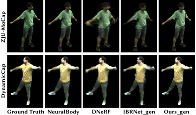
Figure 3. Quantitative results on dynamic scenes. “*_gen” means that these models are directly applied to input images without being additionally fine-tuned on input videos.

3.5. Implementation details

Our generalizable rendering model is trained on an RTX 3090 GPU using Adam (Kingma and Ba, 2015) optimizer with an initial learning rate of $5e^{-4}$ and we half the learning rate every 50k iterations. The model tends to converge after about 200k iterations and it takes about 15 hours. Given an unseen scene, we can finetune our pre-trained model on this scene. Fine-tuning on the new scene generally takes from 10 minutes to 2 hours on an RTX 3090 GPU depending on the number of images. In practice, we sample 64 and 8 depth planes for the coarse-level and fine-level cost volumes, respectively. The proposed rendering model takes from 2 to 3 input source views depending on the number of available cameras. In practice, we set the number of input source views to 2 on dynamic scenes (sparse cameras) and 3 on static scenes (dense cameras) in our experiments. The number of samples per ray is set to 2. We add the sensitivity analysis of number of input views and samples per ray in the supplementary material. The depth ranges for the cost volume is obtained from the structure from motion (Schonberger and Frahm, 2016) algorithm. Please refer to the supplementary material for network structures and other implementation details.

4. Experiments

4.1. Experiments setup

Datasets.

We pre-train our generalizable model using DTU (Jensen et al., 2014) dataset, and take the train-test split and evaluation setting in MVSNeRF, where they select 16 views as seen views and 4 remaining views as novel views for evaluation on each test scene. To further show the generalization ability of our method, we also test the model (trained on DTU) on the NeRF Synthetic and Real Forward-facing (Mildenhall et al., 2020) datasets. They both include 8 complex scenes that have different view distributions from DTU. For dynamic scenes, we evaluate the proposed method on the ZJU-MoCap (Peng et al., 2021b) and DynamicCap (Habermann et al., 2021) datasets. ZJU-MoCap and DynamicCap datasets provide synchronized and calibrated multi-view videos with simple background and high quality masks. For dynamic scenes, we uniformly sample half views as seen views and the other half for testing , and the image resolution is set to $512\times 512$.

Table 1. Quantitative results on dynamic scenes. The time within parentheses represents the training time of the model on the scene. ”0” means that we directly apply the model to the scene without additional fine-tuning. All methods are evaluated on the same machine to report the speed of rendering a $512\times 512$ image. NB denotes NeuralBody.

	ZJU-MoCap			DynamicCap
	PSNR	SSIM	LPIPS	PSNR	SSIM	LPIPS	FPS
NB (10h)	31.85	0.971	0.079	25.35	0.908	0.153	1.297
DNeRF (10h)	26.53	0.889	0.154	22.52	0.826	0.258	0.079
IBRNet (0)	29.46	0.947	0.094	24.67	0.906	0.130	0.517
IBRNet (2h)	32.38	0.968	0.065	25.38	0.900	0.137	0.517
Ours (0)	31.21	0.970	0.041	26.29	0.941	0.068	40.21
Ours (15min)	32.12	0.972	0.037	26.80	0.941	0.065	40.21
Ours (2h)	32.52	0.978	0.030	27.07	0.944	0.059	40.21

Baselines.

As a generalizable radiance field method, we first make comparisons with PixelNeRF (Yu et al., 2021b), IBRNet (Wang et al., 2021b) and MVSNeRF (Chen et al., 2021), which are recent state-of-the-art open source radiance field methods. Then we show that the proposed method with a short fine-tuning process can achieve comparable results with NeRF and other per-scene optimization methods (Wang et al., 2021b; Chen et al., 2021). We follow the same setting as MVSNeRF on above benchmarks and borrow the results of baselines from MVSNeRF. On dynamic scenes, we make comparisons with deformation fields based methods (Pumarola et al., 2021; Zhang et al., 2021) and generalizable radiance field methods (Wang et al., 2021b). We also compare our method with NeuralBody (Peng et al., 2021b). For DNeRF (Pumarola et al., 2021) and NeuralBody, we use their released code and retrained their method under our experimental setting. For IBRNet (Wang et al., 2021b), we use their released code and evaluate their released model pretrained on multiple large-scale datasets under our setting.

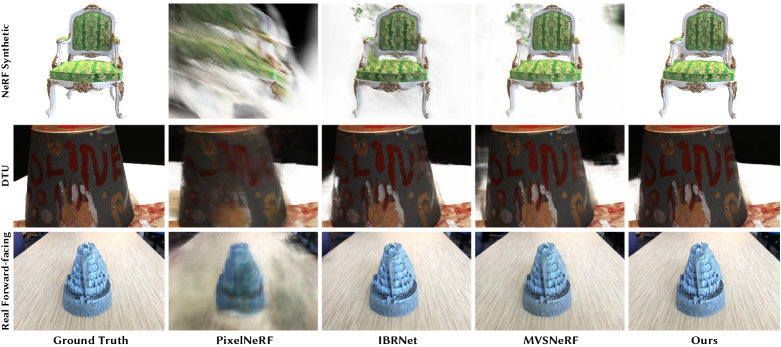
Figure 4. Qualitative comparison of image synthesis results under the generalization setting.

Table 2. Quantitative results of static scenes. “Generalization” means that the model is not additionally fine-tuned. “Per-scene optimization” means that the model is trained or fine-tuned on the target scene. All methods are evaluated on an RTX 3090 GPU to report the speed of rendering a 512 $\times$ 512 image. The results of baselines are borrowed from MVSNeRF.

Methods	Training settings	FPS $\uparrow$	NeRF Synthetic			DTU			Real Forward-facing
			PSNR$\uparrow$	SSIM$\uparrow$	LPIPS$\downarrow$	PSNR$\uparrow$	SSIM$\uparrow$	LPIPS$\downarrow$	PSNR$\uparrow$	SSIM$\uparrow$	LPIPS$\downarrow$
PixelNeRF		0.019	7.39	0.658	0.411	19.31	0.789	0.382	11.24	0.486	0.671
IBRNet	Generalization	0.217	22.44	0.874	0.195	26.04	0.917	0.191	21.79	0.786	0.279
MVSNeRF		0.416	23.62	0.897	0.176	26.63	0.931	0.168	21.93	0.795	0.252
Ours		25.29	26.65	0.947	0.072	27.61	0.956	0.091	22.78	0.808	0.209
NeRF10.2h		0.151	30.63	0.962	0.093	27.01	0.902	0.263	25.97	0.870	0.236
IBRNetft-1.0h	Per-scene optimization	0.217	25.62	0.939	0.111	31.35	0.956	0.131	24.88	0.861	0.189
MVSNeRFft-15min		0.416	27.07	0.931	0.168	28.51	0.933	0.179	25.45	0.877	0.192
Oursft-15min		25.29	27.20	0.951	0.066	28.73	0.956	0.093	24.59	0.857	0.173
Oursft-1.0h		25.29	27.57	0.954	0.063	28.87	0.957	0.090	24.89	0.865	0.159

4.2. Performance on image synthesis

Comparisons on dynamic scenes.

Table 1 lists the quantitative results, which show that our method achieves the state-of-the-art performance with real-time rendering speed. Fig. 3 presents the qualitative results. Note that the length of selected sequences on these datasets are generally from 600 to 1000 frames. We find that DNeRF (Pumarola et al., 2021) has difficulty in handling theses scenes because long sequences have very complex motions. To help DNeRF handle the complex dynamic scenes, we divide the video sequence into several sub-sequences, each of which is separately modeled by a DNeRF network. Please refer to the supplementary material for more details of the setup for baselines.

Comparisons on static scenes.

We report metrics of PSNR, SSIM (Wang et al., 2004) and LPIPS (Zhang et al., 2018) on the NeRF Synthetic, DTU and Real Forward-facing datasets in Table 2. As shown by the quantitative results, our method exhibits competitive performance with baselines with a significant gain in the rendering speed. Note that since PixelNeRF uses a much wider MLP than other methods, it takes almost 10x as much time for rendering compared to other baselines. Fig. 4 and 5 present the qualitative results.

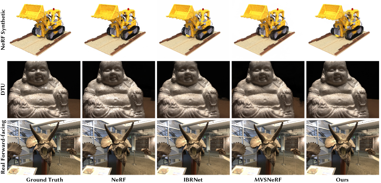
Figure 5. Qualitative comparison of image synthesis results under the per-scene optimization setting.

Table 3. Quantitative comparison of depth results on the DTU dataset. We follow the experimental setting of MVSNeRF and borrow the baseline results from it. MVSNet is trained with depth supervision while other methods are trained with RGB supervision. Abs err means the absolute error. Acc(X) metric is the percentage of pixels whose error is less than X mm.

	Reference view			Novel view
	Abs err	Acc(2)	Acc(10)	Abs err	Acc(2)	Acc(10)
MVSNet	3.60	0.603	0.955	-	-	-
PixelNeRF	49	0.037	0.176	47.8	0.039	0.187
IBRNet	338	0.000	0.913	324	0.000	0.866
MVSNeRF	4.60	0.746	0.913	7.00	0.717	0.866
Ours-MVS	3.80	0.823	0.937	4.80	0.778	0.915
Ours-NeRF	3.80	0.837	0.939	4.60	0.792	0.917

Table 4. Quantitative ablation of the design choices on the DTU dataset. “Depth-gui.” and “Depth-sup.” are “Depth-guided” and “Depth-supervision”, respectively. The rendering resolution here is set to $512\times 640$.

Samples	Depth-gui.	Cascade	Depth-sup.	PSNR$\uparrow$	FPS$\uparrow$
128				27.39	0.630
2				17.75	11.50
2	✓			26.97	9.749
2	✓	✓		27.45	20.31
2	✓	✓	✓	27.11	20.31

4.3. Quality of reconstructed depth

To evaluate the performance of depth prediction, we compare our method with generalizable radiance field methods (Yu et al., 2021b; Wang et al., 2021b; Chen et al., 2021) and the classic MVS method MVSNet (Yao et al., 2018) on the DTU dataset. Denote the depth reconstructed from volume densities as “Ours-NeRF” and the depth produced by the fine-level depth probability volume as “Ours-MVS”. Note that MVSNet is trained with depth supervision while other methods are trained with image supervision. As shown in Table 3, “Ours-NeRF” significantly outperforms baseline methods. Moreover, “Ours-MVS” also produces reasonable depth results from the cost volume. The results show that the proposed sampling strategy facilitate our model to reconstruct better scene geometry than (Wang et al., 2021b; Chen et al., 2021). Please refer to the supplementary material for visual results.

4.4. Ablation studies and analysis

Ablation of main proposed components.

We firstly execute experiments to show the power of depth-guided sampling. As shown in the first three rows of Table 4, when we reduce the number of samples from 128 to 2, the rendering quality of the method without depth-guided sampling drops a lot, while the method with depth-guided sampling can maintain almost the same performance. Secondly, we conduct experiments to analyze the effect of the cascade cost volume. As shown in the fourth row of Table 4, the cascade design greatly improves the rendering speed and shows the same good performance. Note that the non-cascade design has 128 depth planes, while the cascade design has 64 and 8 depth planes. Finally, we additionally supervise the depth probability volume using ground truth depth. As shown in the last row of Table 4, using depth supervision does not improve the rendering performance.

Running time analysis.

To render a $512\times 512$ image, our method with 3 input views and 2 samples per ray runs at 25.21 FPS on a desktop with an RTX 3090 GPU. Specifically, our method takes 4.3 ms to extract image features of 3 input images, 16.1 ms to process the cost volume using 3D CNN, and 19.2 ms for inferring radiance fields and volume rendering.

5. Conclusion and discussion

This paper introduced ENeRF which could support interactive free-viewpoint videos. The core innovation is utilizing explicit depth maps as coarse scene geometry to guide the rendering process of implicit radiance fields. We demonstrated competitive performance of our method among baselines while being significantly faster than previous generalizable radiance field methods.

Although our method can efficiently generate high-quality images, it still has the following limitations. 1) This work focuses on solid surfaces and cannot handle scenes that have multiple surfaces contributing to the appearance, such as transparent scenes. 2) The proposed model generates novel views based on nearby images. Once some target regions under the novel view are invisible in input views, the rendering quality may degrade. It could be solved by considering the visibility of input views.

Supplementary material

In the supplementary material, we provide network architectures, details of experimental setup, and more experimental results.

1. Method details

1.1. Network architectures

Pooling operator.

Given the multi-view point features $\{f_{i}\}_{i=1}^{N}$, the pooling operator $\psi$ aims to aggregate these features to obtain the feature $f_{\text{img}}$, which is used to infer the radiance field. Instead of simply concatenating these features like MVSNeRF (Chen et al., 2021), we use a weighted pooling operator proposed in IBRNet (Wang et al., 2021b), which allows us to input any number of source views. Specifically, we first compute a per-element mean $\boldsymbol{\mu}$ and variance $\mathbf{v}$ of $\{f_{i}\}_{i=1}^{N}$ to capture global information. Then we concatenate each feature $f_{i}$ with $\boldsymbol{\mu}$ and $\mathbf{v}$, and feed the concatenated feature into a small shared MLP to obtain a weight $w_{i}$. The feature $f_{\text{img}}$ is blended via a soft-argmax operator using weights $\{w_{i}\}_{i=1}^{N}$ and multi-view features $\{f_{i}\}_{i=1}^{N}$.

Architectures of MLPs.

The MLP $\phi$ is used to infer the density $\sigma$ from the image feature $f_{\text{img}}$ and the voxel feature $f_{\text{voxel}}$. To predict the color of the point, we use the MLP $\varphi$ to yield the blending weights for image colors in the source views. We illustrate the architectures of $\phi$ and $\varphi$ in Table 5.

1.2. Object-compositional representation

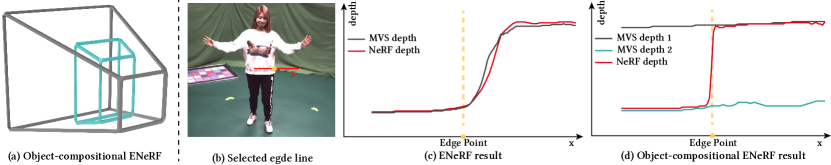
Figure 6. Illustration of compositional ENeRF. (a) To implement compositional ENeRF, we estimate 3D bounding boxes of foreground and background entities, and use ENeRF to separately predict their radiance fields, which are then composited to the full scene’s radiance field. (b) MVS-based depth estimator tends to give smooth predictions that are inaccurate on the edge between the foreground and background. (c) By separately predicting the depth of foreground and background entities, we can sample points around accurate surfaces, thereby enabling NeRF to represent the sharp depth discontinuities.

On complex dynamic scenes (ST-NeRF dataset and outdoor datasets we collected), foreground dynamic objects are usually far away from the background, as shown in Fig. 6 (b). We observe that ENeRF tends to produce artifacts on the border between the foreground objects and the background. The reason is that there exists the depth discontinuities on these regions and our depth estimator tends to produce smooth predictions, resulting in inaccurate depth predictions on edge regions, as shown in Fig. 6 (c). To solve this problem, we introduce the object-compositional representation. Fig. 6 (a) presents an example. Specifically, we first estimate 3D bounding boxes of foreground objects. Then, ENeRF is separately applied to these foreground regions. For simplicity, we assume that the background is static and multi-view background images are given, but our method could also be extended to handle dynamic background. We can use the depth estimator to predict the background depth using the background images. Since the depth estimator of ENeRF is used to predict the depth of foreground and background entities respectively, we can obtain accurate scene geometry and infer radiance fields around correct scene surfaces. Finally, the radiance fields of foreground and background entities are composited. This representation can represent sharp discontinuities and produce accurate depth predictions on the foreground object edge regions, as shown in Fig. 6 (d).

2. Details of the experimental setup

Experimental setup on dynamic scenes.

The evaluation setup on dynamic scenes is taken from NeuralBody (Peng et al., 2021b) and is described as the following. Given the 3D bounding box the dynamic entity, we project it to obtain a bound_mask and make the colors of pixels outside the mask as zero. We compute the PSNR metric for pixels belonging to the bound_mask. To report the SSIM and LPIPS metrics, we first compute the 2D box that bounds the bound_mask and then evaluate the corresponding image region. On the ZJU-MoCap (Peng et al., 2021b) dataset, we select the first 600 frames of Sequence-313. On the DynamicCap (Habermann et al., 2021) dataset, we select the first 1000 frames for Sequence-olek and 600 frames for Sequence-vlad. Note that we do not make comparisons with MVSNeRF (Chen et al., 2021) on dynamic scenes because MVSNeRF use the feature volume when finetuning, which prevent it from handling dynamic scenes.

Experimental setup on static scenes.

Our evaluation setup is taken from MVSNeRF (Chen et al., 2021) and is described as the following. To report the results on the DTU (Jensen et al., 2014) dataset, we compute the metric score of foreground part in images. For metrics of SSIM and LPIPS, we set the background to black and calculate the metric score of the whole image. The segmentation mask is defined by whether there is ground-truth depth available at each pixel. Since marginal regions of images are usually invisible to input images on the Real Forward-facing (Mildenhall et al., 2020) dataset, we only evaluate 80% area in the center of images. The image resolutions are set to $512\times 640$, $640\times 960$ and $800\times 800$ on the DTU, Real forward-facing and NeRF Synthetic (Mildenhall et al., 2020) datasets, respectively.

Table 5. The architectures of MLPs. We denote LR to be LinearRelu layer. “Chns.” shows the number of input and output channels for each layer.

MLP	Layer	Chns.	Input	Output
$\phi$	LR0	8 + 16 / 128	$f_{\text{img}}$, $f_{\text{voxel}}$	hidden feature
	LR1	128 / 64 + 1	hidden feature	$f_{p}$, $\sigma$
$\varphi$	LR0	64 + 16 + 4 / 128	$f_{p}$, $f_{i}$, $\Delta\mathbf{d}_{i}$	hidden feature
	LR1	128 / 64	hidden feature	hidden feature
	LR2	64 / 1	hidden feature	$w_{i}$

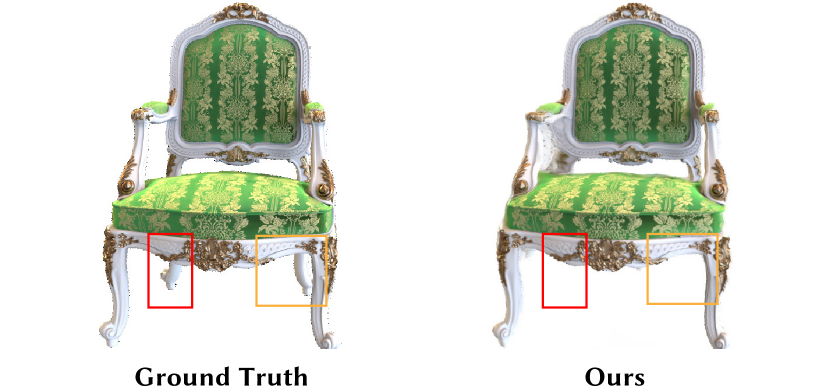
Figure 7. Visual results of artifacts caused by occlusions. In this case, there are some artifacts in the chair legs due to the occlusion.

Experimental setup on the rendering FPS

We report the rendering FPS using the same desktop with an RTX 3090 GPU. The rendering time is defined as network forwarding time. All baselines are implemented using Pytorch. For dynamic scenes, we could further reduce the rendering time by only rendering the image regions in the bound_mask defined in the last section (Experimental setup on dynamic scenes). This improves the rendering FPS from 30.57 to 40.21. Note that all baselines on the dynamic scenes utilize this trick to ensure the comparison fairness. The rendering FPS of free-viewpoint video demos in the video extraly includes the data loading and interactive GUI time. All processes in the interactive demos are implemented with python and the GPU utilization is generally from 70 to 80 %. This indicates our method may achieve higher speeds with a more efficient implementation.

Experimental details of DNeRF

we found simply applying DNeRF (Pumarola et al., 2021) on benchmark datasets cannot converge because benchmark datasets exhibit complex motions. To obtain a reasonable result for DNeRF, we train 2 models for the Sequence-313 on the ZJU-MoCap dataset. On the DynamicCap dataset, we train 10 and 12 models for Sequence-olek and Sequence-vlad, respectively. Specifically, for the Sequence-vlad of 600 frames, training 12 models means that each model is trained on 50 frames.

3. More experimental results

Table 6. Quantitative ablation analysis of the number of samples and input source views on the DTU dataset.

Samples	PSNR$\uparrow$	FPS$\uparrow$	Views	PSNR$\uparrow$	FPS$\uparrow$
1	26.89	26.01	2	25.45	24.91
2	27.45	20.01	3	27.45	20.01
4	27.49	13.42	4	27.80	16.73
8	27.54	8.09	5	27.84	14.32

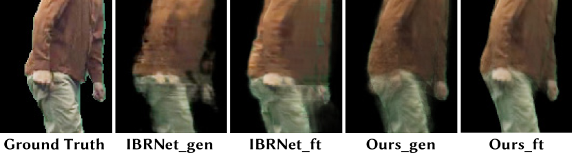
Figure 8. Zoom-in results on the DynamicCap dataset. Our method renders more appearance details than baseline methods. After short-term finetuning, the proposed method produces better rendering results.

Visual results of artifacts caused by occlusions.

As discussed in section 5, our method may have artifacts in occluded regions. We provide visual results on the NeRF Synthetic dataset under the generalization setting in Fig. 7 to identify these artifacts.

Visual results of fine-tuning models on dynamic scenes.

We include the visual results of fine-tuning models on ZJU-MoCap and DynamicCap datasets in Fig. 9 and zoom-in results in Fig. 8. Our method exhibits better performance after fine-tuning on the target sequence.

Visual depth results.

As shown in Figure 10, the proposed method produces reasonable depth results by supervising networks with only RGB images. The cost volume recovers high-quality depth, which allows us to place few samples around the surface to achieve photorealistic view synthesis.

Visual ablation results.

We provide visual ablation results in Figure 11. The results show that when we reduce the number of samples from 128 to 2, our method with depth-guided sampling almost maintains the same rendering quality. With the depth-guided sampling, the construction of a high-resolution cost volume becomes a bottleneck in the rendering speed. The cascade cost volume further speeds up the construction of the cost volume without loss of rendering quality as shown in Figure 11.

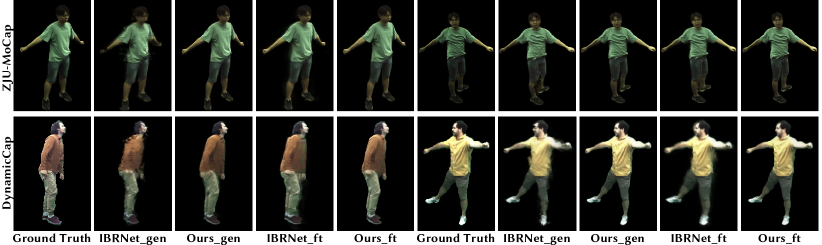
Figure 9. Quantitative results on the ZJU-MoCap and DynamicCap datasets. “IBRNet_gen” and “Ours_gen” mean that these models are directly applied to input images without be additionally fine-tuned on input videos. “IBRNet_ft” and “Ours_ft” mean that these models are finetuned on the target sequence.

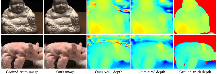
Figure 10. Visual depth results on the DTU dataset. “Ours NeRF depth” represents the depth results recovered from volume densities. “Ours MVS depth” denotes the depth results from the fine-level cost volume.

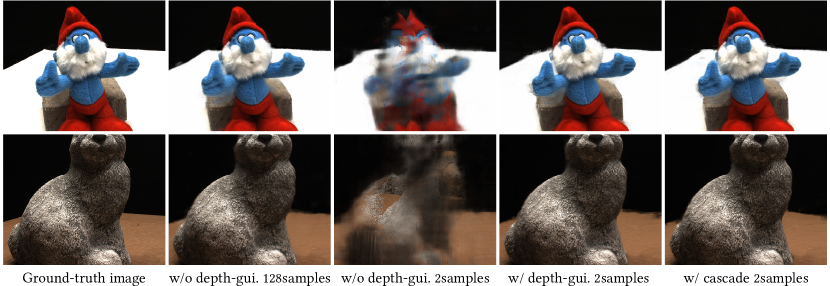
Figure 11. Visual ablation results on the DTU dataset. “w/o depth-gui.” is similar to MVSNeRF (Chen et al., 2021).

Sensitivity analysis.

We provide sensitivity analysis on the number of input views and the number of samples per ray in Table 6. On the DTU dataset, we found 3 views and 2 sampling points can produce high quality view synthesis results at interactive frame rates.

Ablation on the rendering head.

As stated in the main paper, we predict the blend weights for source view RGBs to obtain the final radiance like (Wang et al., 2021b). Alternatively, we can also output the final radiance simply by predicting the radiance from the volume and image feature like (Chen et al., 2021). The results are 26.77/0.95 in terms of PSNR/SSIM metrics when using the rendering head in  (Chen et al., 2021), while they are 27.88/0.96 when using the rendering head in  (Wang et al., 2021b).

Ablation on the depth range hyperparameter $\lambda$.

We experimentally found that setting $\lambda=1$ produces good results. One optional design maybe progressively reduce the $\lambda$ from 3 to 1 during training. This design produces lower performance than the taken design (PSNR/SSIM = 25.25/0.89 v.s. 27.61/0.96).

Perceptual loss.

We find that the perceptual loss largely affects the LPIPS metric but has little effect on PSNR and SSIM metrics. Specifically, the model trained with $\mathcal{L}_{perc}$ gives 27.62/0.956/0.091 on the DTU dataset in terms of PSNR/SSIM/LPIPS metrics, while the one without $\mathcal{L}_{perc}$ gives 27.88/0.955/0.106.

Comparisons with NeuralRays (Liu et al., 2021b)

. We provide qualitative comparisons with NeuralRays under the experimental setting taken in their paper where various large-scale datasets are used during pretraining. Our method presents competitive performance while runs significantly faster than their method on the Real Forward-facing dataset.(Ours:25.71/8.42 v.s. NeuralRays:25.35/0.03 in terms of PSNR/FPS@756x1008; the performance is from their paper and the speed is tested using their released code).

Table 7. Quantitative comparison on the DTU dataset.

Scan	#1	#8	#21	#103	#114
Metric	PSNR$\uparrow$
PixelNeRF	21.64	23.70	16.04	16.76	18.40
IBRNet	25.97	27.45	20.94	27.91	27.91
MVSNeRF	26.96	27.43	21.55	29.25	27.99
Ours	28.85	29.05	22.53	30.51	28.86
NeRF10.2h	26.62	28.33	23.24	30.40	26.47
IBRNetft-1h	31.00	32.46	27.88	34.40	31.00
MVSNeRFft-15min	28.05	28.88	24.87	32.23	28.47
Oursft-15min	29.81	30.06	22.50	31.57	29.72
Oursft-1h	30.10	30.50	22.46	31.42	29.87
Metric	SSIM$\uparrow$
PixelNeRF	0.827	0.829	0.691	0.836	0.763
IBRNet	0.918	0.903	0.873	0.950	0.943
MVSNeRF	0.937	0.922	0.890	0.962	0.949
Ours	0.958	0.955	0.916	0.968	0.961
NeRF10.2h	0.902	0.876	0.874	0.944	0.913
IBRNetft-1h	0.955	0.945	0.947	0.968	0.964
MVSNeRFft-15min	0.934	0.900	0.922	0.964	0.945
Oursft-15min	0.964	0.958	0.922	0.971	0.965
Oursft-1h	0.966	0.959	0.924	0.971	0.965
Metric	LPIPS $\downarrow$
PixelNeRF	0.373	0.384	0.407	0.376	0.372
IBRNet	0.190	0.252	0.179	0.195	0.136
MVSNeRF	0.155	0.220	0.166	0.165	0.135
Ours	0.086	0.119	0.107	0.107	0.076
NeRF10.2h	0.265	0.321	0.246	0.256	0.225
IBRNetft-1h	0.129	0.170	0.104	0.156	0.099
MVSNeRFft-15min	0.171	0.261	0.142	0.170	0.153
Oursft-20min	0.074	0.109	0.100	0.103	0.075
Oursft-1h	0.071	0.106	0.097	0.102	0.074

4. Discussions

Learning the depth prediction with the rendering loss. We found that the depth prediction network can give good results even when we only sample one point during the volume rendering. This is interesting, because backpropagating gradient through only one point may make the training of the depth prediction easily trapped in the local optimum. A possible reason is that the depth is estimated using the softargmax of depth probability volume and gradients are backpropagated to the depth planes during training. This regularizes the optimization process and helps the depth prediction network to converge to the global optimum. To validate this assumption, we design a baseline by replacing the depth prediction network in our model with an MLP network, which takes the spatial coordinate and viewing direction as input and outputs the distance to the surface. In contrast to our model, this baseline does not converge well and obtains bad rendering results.

Performance of PixelNeRF (Yu et al., 2021b).

We found that PixelNeRF gives bad performance on the NeRF Synthetic and Real Forward-facing datasets. One reason is that PixelNeRF takes absolute XYZ coordinates as input and is trained on the DTU dataset. Since the coordinate system of the DTU dataset is quite different from that of NeRF synthetic and Real Forward-facing datasets, PixelNeRF cannot generalize well on these two datasets. MVSNeRF (Chen et al., 2021) also reported that PixelNeRF performs poor on the NeRF Synthetic and Real Forward-facing datasets. Our method takes image features and volume features as input, thereby achieving a better generalization ability.

More discussions on the limitations.

In addition to the limitations we have discussed in the main paper, we here provide more discussions. Our method may fail to render high-quality results in scenes including multi-surface, fuzzy, specular highlight and semi-transparent regions. This is because the MVS generally fails to recover the correct depth in these regions. Incorporating a layered representation (Zhang et al., 2021) maybe helpful and we leave it as the future work.

5. Per-scene breakdown

Tables 7, 8 and 9 present the per-scene comparisons. These results are consistent with the averaged results in the paper and show that our method achieves comparable performance to baselines.

Table 8. Quantitative comparison on the NeRF Synthetic dataset.

	Chair	Drums	Ficus	Hotdog	Lego	Materials	Mic	Ship
Metric	PSNR$\uparrow$
PixelNeRF	7.18	8.15	6.61	6.80	7.74	7.61	7.71	7.30
IBRNet	24.20	18.63	21.59	27.70	22.01	20.91	22.10	22.36
MVSNeRF	23.35	20.71	21.98	28.44	23.18	20.05	22.62	23.35
Ours	28.44	24.55	23.86	34.64	24.98	24.04	26.60	26.09
NeRF	31.07	25.46	29.73	34.63	32.66	30.22	31.81	29.49
IBRNetft-1h	28.18	21.93	25.01	31.48	25.34	24.27	27.29	21.48
MVSNeRFft-15min	26.80	22.48	26.24	32.65	26.62	25.28	29.78	26.73
Oursft-15min	28.52	25.09	24.38	35.26	25.31	24.91	28.17	25.95
Oursft-1h	28.94	25.33	24.71	35.63	25.39	24.98	29.25	26.36
Metric	SSIM$\uparrow$
PixelNeRF	0.624	0.670	0.669	0.669	0.671	0.644	0.729	0.584
IBRNet	0.888	0.836	0.881	0.923	0.874	0.872	0.927	0.794
MVSNeRF	0.876	0.886	0.898	0.962	0.902	0.893	0.923	0.886
Ours	0.966	0.953	0.931	0.982	0.949	0.937	0.971	0.893
NeRF	0.971	0.943	0.969	0.980	0.975	0.968	0.981	0.908
IBRNetft-1h	0.955	0.913	0.940	0.978	0.940	0.937	0.974	0.877
MVSNeRFft-15min	0.934	0.898	0.944	0.971	0.924	0.927	0.970	0.879
Oursft-15min	0.968	0.958	0.936	0.984	0.948	0.946	0.981	0.891
Oursft-1h	0.971	0.960	0.939	0.985	0.949	0.947	0.985	0.893
Metric	LPIPS $\downarrow$
PixelNeRF	0.386	0.421	0.335	0.433	0.427	0.432	0.329	0.526
IBRNet	0.144	0.241	0.159	0.175	0.202	0.164	0.103	0.369
MVSNeRF	0.282	0.187	0.211	0.173	0.204	0.216	0.177	0.244
Ours	0.043	0.056	0.072	0.039	0.075	0.073	0.040	0.181
NeRF	0.055	0.101	0.047	0.089	0.054	0.105	0.033	0.263
IBRNetft-1h	0.079	0.133	0.082	0.093	0.105	0.093	0.040	0.257
MVSNeRFft-15min	0.129	0.197	0.171	0.094	0.176	0.167	0.117	0.294
Oursft-15min	0.033	0.047	0.069	0.031	0.073	0.063	0.021	0.190
Oursft-1h	0.030	0.045	0.071	0.028	0.070	0.059	0.017	0.183

Table 9. Quantitative comparison on the Real Forward-facing dataset.

	Fern	Flower	Fortress	Horns	Leaves	Orchids	Room	Trex
	PSNR$\uparrow$
PixelNeRF	12.40	10.00	14.07	11.07	9.85	9.62	11.75	10.55
IBRNet	20.83	22.38	27.67	22.06	18.75	15.29	27.26	20.06
MVSNeRF	21.15	24.74	26.03	23.57	17.51	17.85	26.95	23.20
Ours	20.88	24.78	28.63	23.51	17.78	17.34	28.94	20.37
NeRF10.2h	23.87	26.84	31.37	25.96	21.21	19.81	33.54	25.19
IBRNetft-1h	22.64	26.55	30.34	25.01	22.07	19.01	31.05	22.34
MVSNeRFft-15min	23.10	27.23	30.43	26.35	21.54	20.51	30.12	24.32
Oursft-15min	21.84	27.46	29.58	24.97	20.95	19.17	29.73	23.01
Oursft-1h	22.08	27.74	29.58	25.50	21.26	19.50	30.07	23.39
	SSIM$\uparrow$
PixelNeRF	0.531	0.433	0.674	0.516	0.268	0.317	0.691	0.458
IBRNet	0.710	0.854	0.894	0.840	0.705	0.571	0.950	0.768
MVSNeRF	0.638	0.888	0.872	0.868	0.667	0.657	0.951	0.868
Ours	0.727	0.890	0.920	0.866	0.685	0.637	0.958	0.778
NeRF10.2h	0.828	0.897	0.945	0.900	0.792	0.721	0.978	0.899
IBRNetft-1h	0.774	0.909	0.937	0.904	0.843	0.705	0.972	0.842
MVSNeRFft-15min	0.795	0.912	0.943	0.917	0.826	0.732	0.966	0.895
Oursft-15min	0.758	0.919	0.940	0.893	0.816	0.710	0.963	0.855
Oursft-1h	0.770	0.923	0.940	0.904	0.827	0.725	0.965	0.869
	LPIPS $\downarrow$
	Fern	Flower	Fortress	Horns	Leaves	Orchids	Room	Trex
PixelNeRF	0.650	0.708	0.608	0.705	0.695	0.721	0.611	0.667
IBRNet	0.349	0.224	0.196	0.285	0.292	0.413	0.161	0.314
MVSNeRF	0.238	0.196	0.208	0.237	0.313	0.274	0.172	0.184
Ours	0.235	0.168	0.118	0.200	0.245	0.308	0.141	0.259
NeRF10.2h	0.291	0.176	0.147	0.247	0.301	0.321	0.157	0.245
IBRNetft-1h	0.266	0.146	0.133	0.190	0.180	0.286	0.089	0.222
MVSNeRFft-15min	0.253	0.143	0.134	0.188	0.222	0.258	0.149	0.187
Oursft-15min	0.220	0.130	0.103	0.177	0.181	0.266	0.123	0.183
Oursft-1h	0.197	0.121	0.101	0.155	0.168	0.247	0.113	0.169