Hierarchical clustering: visualization, feature importance and model selection

Abstract

We propose methods for the analysis of hierarchical clustering that fully use the multi-resolution structure provided by a dendrogram. Specifically, we propose a loss for choosing between clustering methods, a feature importance score and a graphical tool for visualizing the segmentation of features in a dendrogram. Current approaches to these tasks lead to loss of information since they require the user to generate a single partition of the instances by cutting the dendrogram at a specified level. Our proposed methods, instead, use the full structure of the dendrogram. The key insight behind the proposed methods is to view a dendrogram as a phylogeny. This analogy permits the assignment of a feature value to each internal node of a tree through an evolutionary model. Real and simulated datasets provide evidence that our proposed framework has desirable outcomes and gives more insights than state-of-art approaches. We provide an R package that implements our methods.

1 Introduction

Clustering methods have the goal of grouping similar sample points. They are used in applications such as pattern recognition (Chen et al.,, 2014), image analysis (Rocha et al.,, 2009), bioinformatics (Datta and Datta,, 2003), and information retrieval (Jardine and van Rijsbergen,, 1971).

Clustering techniques can be divided into two categories: partition-based and hierarchical. An example of partition-based clustering is K-means (MacQueen,, 1967), which creates $K$ clusters based on a Voronoi partition of the feature space. Similarly, mode-based clustering (Fukunaga and Hostetler,, 1975) creates a partition by assigning each observation to a mode of a density estimate. On the other hand, hierarchical clustering yields a tree-based representation of the objects (dendrogram), such as in agglomerative clustering (Ward Jr,, 1963), DIANA (Rousseeuw and Kaufman,, 1990) and partial least squares methods (Liu et al.,, 2006). This paper focuses solely on hierarchical clustering.

Hierarchical clustering has some advantages when compared to partition-based clustering. For instance, it does not require the specification of the number of clusters. Also, as shown in fig. 1, a dendrogram displays a general similarity structure of the data by providing a multiresolution view. The lower in the dendrogram that two observations are merged, the more similar they are. By using this similarity structure, fig. 1 illustrates how to obtain a partition by cutting a dendrogram at a given height.

However, there exist challenging questions when implementing hierarchical clustering. For instance, how does one choose a particular hierarchical clustering method among the many that are available? (question 1) Specifically, how can the performance of a dendrogram be evaluated? Also, after a clustering method is chosen, how do the available features relate to the dendrogram? For example, how can the position of each sample in the dendrogram be explained in terms of its feature values? (question 2) Also, which features are best segmented by the dendrogram? (question 3)

Novelty. To the best of our knowledge, our framework is the first one to address the above questions by utilizing the full hierarchical structure provided by the dendrogram. Unlike current approaches, which require the user to generate a partition by cutting the dendrogram at a specified level (Datta and Datta,, 2003; Hubert and Arabie,, 1985; Rosenberg and Hirschberg,, 2007; Yeung et al.,, 2001; Kassambara,, 2017; Seo and Shneiderman,, 2002; Galili,, 2015; Ismaili et al.,, 2014; Badih et al.,, 2019), our approach makes use of the richer structure provided by the dendrogram and does not restrict itself to a single partition, thus avoiding loss of information, as demonstrated in section 5.

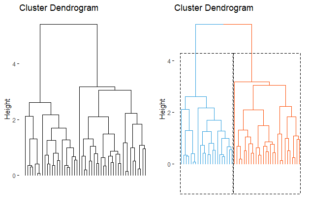
Figure 1: (Left) Dendrogram obtained from hierarchical clustering with average linkage. (Right) By cutting the dendrogram at height 4, two clusters are obtained.

1.1 Overview of the method

We answer the questions in the last section through probabilistic evolutionary models commonly used in phylogenetic analysis (Joy et al.,, 2016; Pupko and Mayrose,, 2020; Borges et al.,, 2021). The key insight in this framework is to view a dendrogram as a phylogeny. This metaphor is helpful since the phylogeny is associated to a probabilistic evolutionary model.

Probabilistic evolutionary models describe how each characteristic evolves over a phylogeny. In the context of hierarchical unsupervised learning, this translates into modeling how a feature evolves over a dendrogram using phylogeny information and feature data. These models predict feature values for leaves of the dendrogram and also for internal nodes, a task known as ancestral state reconstruction. This reconstruction allow one to visualize each feature’s segmentation by the dendrogram, thus providing an answer to (2). Also the evolutionary model’s predictions provide a measure for the accuracy of each dendrogram. By adapting ideas from cross-validation, we obtain a loss used for dendrogram selection, thus answering question (1). Finally, feature importance is associated to how well the probabilistic evolutionary model predicts that feature, which answers question (3).

We illustate our approach using the ceramic samples dataset, which contains information about the chemical composition of 88 ceramic samples. This dataset contains 17 features, each related to the percentage of certain chemical compound present in each sample (e.g., AL₂O₃ (Aluminium Oxide), CaO (Calcium Oxide), etc). The table in fig. 2(a) provides the hierarhical clustering prediction loss for a few clustering methods. This loss provides an immediate way of comparing the performance of the methods. For instance, since McQuitty has the lowest loss, it has the highest performance in this dataset, closely followed by average linkage. Also, fig. 2(b) illustrates the feature importance score. While AL₂O₃, SrO and CaO are the most relevant features in the construction of the dendrogram, MgO, CuO and ZnO are the least important ones. Finally, fig. 2(c) illustrates how the hierarquical structure explains the distribution behaviour of each feature. The left dendrogram shows that Al₂O₃ is well segmented by the dendrogram, as explained by the even color distribution among its major branches. That is, while 2 major clusters are characterized by low values for AL₂O₃, a third major cluster is characterized by high values of AL₂O₃. The right dendrogram shows that MgO is not so well explained by the dendrogram, since its major branches contain a high variability of colors. None of the illustrations required us to fix the number of clusters.

Method	McQuitty	Average linkage	Diana	Ward D	Single linkage
Loss	0.545	0.546	0.561	0.578	0.651

(a) Cross-validated loss (CVL) indicates which hierarchical clustering method to use. In this case, McQuitty has the best performance.

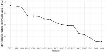
(b) Phylogenetic feature importance score (PFIS) shows the importance of each feature in Mcquitty dendrogram.

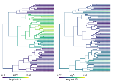
(c) Evolutionary dendrograms gives insights about the clustering by describing how each feature behaves in each internal node.

Figure 2: Illustration of the proposed hierarchical clustering methodology to the ceramic dataset. In panel (a), the prediction loss measures how well each hierarchical clustering method explains the data. In this example, McQuitty is the best method. In panel (b), the feature importance score determines which of the features are best explained by the McQuitty dendrogram. While Al₂O₃ is the best explained by the dendrogram, MgO is the least explained. In panel (c), the evolutionary dendrograms for Al₂O₃ (left) and MgO (right) provide insights on how the hierarchical structure explains the behaviour of each of these feature.

This work is organized as follows: Section 2 reviews hieararchical clustering and probabilistic evolutionary models, section 3 formulates and explains our methodology, section 4 outlines related approaches, and section 5 shows experimental results.

2 The relation between hierarchical clustering and probabilistic evolutionary models

Hierarchical clustering and phylogenetics share a common trait: dendrograms and phylogenies are both formalized as trees. That is, the difference between a dendrogram and a phylogeny is given solely by the context in which it is used. While a dendrogram is used to specify the similarity structure between instances, the phylogeny describes evolutionary relationships. Since both types of analysis share a common formalism, it is possible to adapt the methods of one to the other.

Based on this shared formalism, we also use a common notation for describing the elements of a tree. The left panel in fig. 1 depicts a tree. The nodes at the bottom of the tree are called leaves. These leaves often represent instances in the dataset. As one moves up the tree, the leaves merge into internal nodes, and then internal nodes merge with one another until the root is reached at the top of the tree. The descendants of a node are the leaves that stem from it.

The following subsections briefly review hierarchical clustering and phylogenetical evolutionary models.

2.1 Hierarchical methods

Hierarchical clustering methods yield a tree-based representation of the data named dendrogram, as illustrated in Figure 1. In clustering, a node is often interpreted as the group of instances which are its descendants. The earlier a merge between two nodes, the more similar are the corresponding groups of descendants (James et al.,, 2013).

Using the dendrogram, it is possible to partition the instances according to their similarity. Such a partition is obtained by cutting the dendrogram with a horizontal line at a given height, as shown on the right panel of Figure 1. While cutting at lower heights obtains groups with a greater similarity, cutting at higher heights obtains a smaller number of groups. A trade-off between these properties yields the most interpretable partition.

Hierarchical clustering methods can be divided into two paradigms: agglomerative (bottom-up) and divisive (top-down) (Hastie et al., 2009a, ). Agglomerative strategies start at the leaves of the dendrogram, iteratively merging selected pairs of branches until the root of the tree is reached. The pair of branches chosen for merging is the one that has the smallest measurement of intergroup dissimilarity. Divisive methods start at the root at the root of the tree. Such methods iteratively divide a chosen branch into smaller ones until the leaves are obtained. The splitting criterion maximizes a measure of between-group dissimilarity.

2.2 Evolutionary models and ancestral state reconstruction in phylogenetics

A phylogeny represents the evolutionary relationships among instances based on similarities in their features (traits) (Felsenstein,, 1985). Each leaf of a tree often represents, for example, a specimen, a species or a family. In this context, an internal node is interpreted as the most recent common ancestor of its descendants.

It is often reasonable to posit that these ancestors have unobserved feature values. In this context, ancestral state reconstruction is the task of estimating unobserved feature values using phylogenetic evolutionary models based on the phylogeny and feature values in the dataset. This reconstruction is performed by probabilistic evolutionary methods like SIMMAP (Bollback,, 2006), for categorical features and by methods based on Brownian motion (O’Meara et al.,, 2006; Clavel et al.,, 2015; Revell,, 2012), for continuous features. These models can also provide feature value predictions at the leaves.

The ancestral state reconstruction performed by these evolutionary methods are illustrated in Figure 5, which was obtained using the phytools package (Revell,, 2012). Figure 3 illustrates ancestral state reconstruction for a categorical binary feature. The pie chart over each node is the estimated probability distribution of its feature value. Figure 4 illustrates ancestral state reconstruction for a continuous feature. The color of each node represents the expected value of its feature value. In this case, the expected value of the feature along the edges can be calculated using a Brownian motion model.

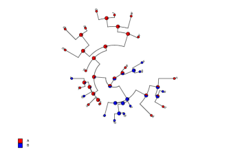
Figure 3: Categorical feature

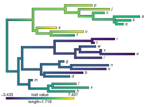
Figure 4: Continuous feature

Figure 5: Illustration of ancestral state reconstruction methods.

3 Methodology

Since both dendrograms and phylogenies are formally represented by a tree, it is possible to use common interpretations and intuition of one in the other. In particular, it is useful to interpret an internal node of a dendrogram as an ancestor or an archetype of its descendants. Using this point of view, one can fit evolutionary models to hierarchical clustering and perform ancestral state recognition together with leaf prediction. The following subsections describe some of the benefits of this point of view. Subsection 3.1 shows useful graphical representations based on ancestral state reconstruction named evolutionary dendrograms. Subsections 3.2 and 3.3 show how this connection leads, respectively, to a loss for clustering methods (CVL) and to a measure for feature importance (PFIS) in a dendrogram.

These tools can be combined into a complete hierarchical clustering analysis framework as shown in the flowchart of Figure 6. First, we fit all hierarchical clustering methods we desire based on the input data. Next, for each dendrogram, an evolutionary model predicts each feature’s values through a leave-one-feature-out strategy. These predictions yield a loss (CVL) for each dendrogram, thus allowing the selection of the one with best perfomance. For the selected dendrogram, we compute feature importance score using PFIS. This score uses the evolutionary model and a leave-one-observation-out strategy to determine how well each feature is explained by the dendrogram. We also visualize how the chosen dendrogram explains each feature using the probabilistic evolutionary model. This model uses ancestral state reconstruction to plot how each feature evolves over the dendrogram.

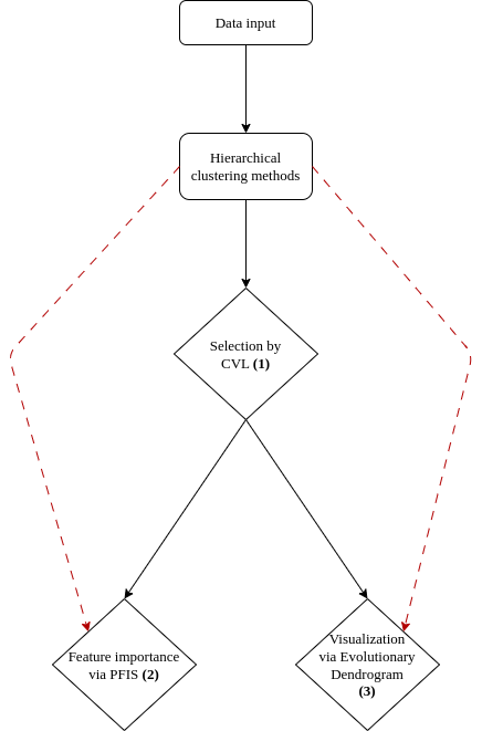
Figure 6: Flowchart of our full (only continuous arrows) and partial (dashed arrows) framework. The numbers displayed in parenthesis show which question each step answers. The full framework selects the best performing hierarchical clustering method according to our proposed loss (CVL). Afterwards, both feature importance (PFIS) and evolutionary dendrograms are plotted to provide insights and to better explain the dendrogram that was selected by CVL. If we already have a single hierarchical method, the selection step can be skipped and we can proceed directly to plotting feature importance and evolutionary dendrograms, as indicated by the dashed arrows.

In what follows, we denote the dataset by

$$\mathbb{D}=\left[x_{i,j}\right]_{i=1,\ldots,n}^{j=1,\ldots,p},$$

where $i$ indexes the instances, and $j$ indexes the features. Also, we denote a dendrogram by ${\mathcal{T}}$. When we want to emphasize that ${\mathcal{T}}$ is built using data $\mathbb{D}$, we denote it by $\hat{{\mathcal{T}}}$.

3.1 Evolutionary dendrograms

By interpreting a dendrogram as a phylogeny, one can fit a probabilistic evolutionary model to the dendrogram and obtain insights about the clustering through ancestral state reconstruction. This approach offers a multiresolution visualization of the data, which does not require a pre-specified number of clusters. More specifically, this approach describes how each feature behaves in each internal node of the dendrogram. Such a visualization provides insight about what partition size yields a more useful description of the data.

Because ancestral state reconstruction visualization tools are already implemented in phylogenetic analysis packages like phytools (Revell,, 2012) and ape (Paradis and Schliep,, 2019) both for continuous and categorical traits, it is straightforward to apply these methods to the hierarchical clustering context: one only needs to take the resulting dendrogram as the input for these procedures. We provide code for this simple adaptation in https://github.com/Monoxido45/PhyloHclust and illustrate this graphical analysis with an application to the USArrests (McNeil,, 1977) and Iris (Fisher,, 1936) datasets.

3.1.1 Evolutionary dendrograms applied to the USArrests dataset

The USArrests dataset (McNeil,, 1977) describes the urban population and murder, assault and rape rates per 100,000 residents for each of the USA states. Using this data, we obtain a dendrogram for the USA states using the McQuitty method and perform ancestral state reconstruction applying a fitted Brownian Motion evolution model along the edges (Felsenstein,, 1985; Revell,, 2012, 2013). Figure 7 shows the evolutionary dendrograms for standardized Murder (top left), Assault (top right) and Rape (bottom right) rates per 100.000 residents and standardized Urban population (bottom left). Through the evolutionary dendrogram, we can obtain valuable insights, such as the following:

• Since the major branches of the top dendrograms have similarly colored descendants in both cases, both Assault and Murder features are well segmented by the dendrogram.

• In the top left dendrogram, the major internal nodes vary from high (yellow) to low murder rates (dark blue), with high Murder rates descendant states listed from South Carolina to Louisiana, medium murder rates (green) from New Mexico to Alaska, mild to low rates (light blue) from Utah to Arkansas, low rates (dark blue) from New Hamsphire to South Dakota.

• In the right dendrogram, Assault rates are segmented in a similar way as Murder’s dendrogram. The main difference from the previous analysis is that high assault rates are not well separated from medium assault rates.

• One might use a coarse partition which divides the states into three groups: one with medium to high murder and attack rates, another with mild rates, and the last with low rates. Furthermore, one could also refine the partition by dividing the first group into two others with respectively high and medium murder rates.

• The deep internal nodes of Rape rate dendrogram are colored similarly to Assault rate dendrogram. That is, these features are segmented similarly by the dendrogram.

• Urban population is not well segmented by the dendrogram: the major branches of the Urban Population dendrogram have differently colored descendants, and almost all of its deep internal nodes are green. Thus, we could obtain more internally homogeneous groups by selecting internal nodes that are closer to the leaves, but these groups would be similar to others that are not in the same major branch. For instance, we can select internal nodes in the first major branch with descendants listed from South Carolina to Lousiana and internal nodes in the second major branch with descendants listed from New Hamsphire to South Dakota.

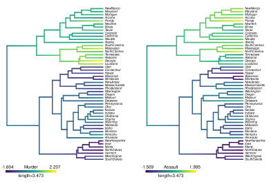
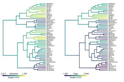
Figure 7: Evolutionary dendrograms for standardized Murder (top left), Assault (top right) and Rape (bottom right) rates per 100.000 residents and standardized Urban population (bottom left) applied to a clustering obtained using the McQuitty method.

It would be much harder to perform the above analysis directly through a standard partition-based boxplot analysis. One would need to cut the dendrogram at several different heights and then gather the collection of boxplots obtained for each feature and heigth. By doing so, the multi-resolution view offered by the dendrogram is lost and clustering cannot be visualized at an individual level. We further detail this comparison in Section 5.1.

3.1.2 Evolutionary dendrograms applied to the Iris dataset

The Iris dataset (Fisher,, 1936) contains measurements related to $150$ flowers. Specifically, it contains the width and length of the sepals and petals of flowers which are classified into three species: setosa, versicolor, and virginica. In this analysis, we performed clustering using complete linkage over the petal and sepal measurements.

Although the species were not used in the clustering, a graphical analysis shows how well the resulting dendrogram segments this label. Figure 8 illustrates the evolutionary dendrogram for species using SIMMAP (Bollback,, 2006). The Figure shows that, using a partition of size $5$, the dendrogram segments the label adequately.

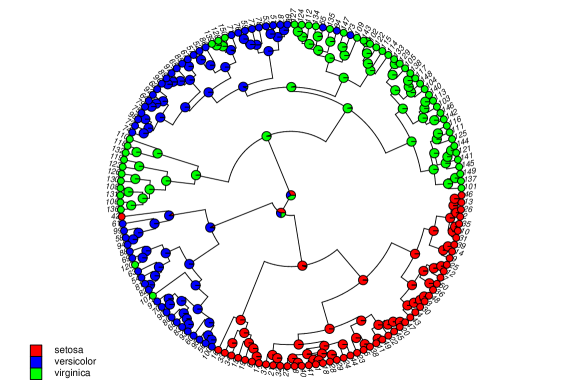
Figure 8: Evolutionary dendrogram obtained by applying acenstral state reconstruction of species based on the SIMMAP algorithm. The original dendrogram is obtained by performing complete linkage clustering to petal and sepal widths and heights.

3.2 Cross-validated loss (CVL)

Before one can interpret a dendrogram, it is necessary to choose a clustering algorithm. In order to do this, we propose a new loss function for evaluating the performance of each algorithm.

The connection between dendrograms and phylogenies can also be explored for choosing between clustering algorithms. The main advantage of this relation is that a phylogeny induces predictions over instances. As a result, it is possible to adapt to clustering the methods for model selection that are used in supervised learning. More specifically, our proposal is an adaptation of a leave-one-feature-out cross-validation approach for selecting phylogenies (Borges et al.,, 2021). Let $\hat{{\mathcal{T}}}$ be a dendrogram fitted according to an arbitrary method. The score is given by

$$\mbox{CVL}(\hat{{\mathcal{T}}}):=p^{-1}\sum_{j=1}^{p}L_{j}(\hat{{\mathcal{T}}}_{-j}),$$

where

$$L_{j}(\hat{{\mathcal{T}}}_{-j}):=n^{-1}\sum_{i=1}^{n}d_{j}(\hat{x}_{i,j},x_{i,j}),$$

$\hat{{\mathcal{T}}}_{-j}$ is the dendrogram fitted according to the same method, but without the $j$-th feature, $\hat{x}_{i,j}$ is a prediction $\hat{{\mathcal{T}}}_{-j}$ gives to $x_{i,j}$, the $j$-th feature of the $i$-th instance, and $d_{j}(\hat{x}_{i,j},x_{i,j})$ as the inaccuracy of $\hat{x}_{i,j}$ with respect to $x_{i,j}$. The proposal is summarized in Algorithm 1. For Algorithm 1 to be operational, it is necessary to choose a prediction function and a measure of inaccuracy of predictions. The choice of these functions depends on whether the feature under analysis is categorical or continuous.

Algorithm 1 Cross-validation loss (CVL)

Input: Clustering algorithm, $\hat{{\mathcal{T}}}$, and data $x_{i,j}$, for $1\leq i\leq n$ and $1\leq j\leq p$.
Output: CVL($\hat{{\mathcal{T}}}$), the cross-validated predictive loss of $\hat{{\mathcal{T}}}$.

1:for each feature, $j$, do

2:     Let $\hat{{\mathcal{T}}}_{-j}$ be obtained by applying $\hat{{\mathcal{T}}}$ to the data with feature $j$ removed.

3:     for each instance, $i$, do

4:         Let $\hat{x}_{i,j}$ be a prediction for $x_{i,j}$ based on $\hat{{\mathcal{T}}}_{-j}$ and on $x_{i^{\prime},j}$ for $i^{\prime}\neq i$.

5:         Let $d_{j}(\hat{x}_{i,j},x_{i,j})$ measure how inaccurate prediction $\hat{x}_{i,j}$ is for $x_{i,j}$.

6:     end for

7:     Let $L_{j}(\hat{{\mathcal{T}}}_{-j}):=n^{-1}\sum_{i=1}^{n}d_{j}(\hat{x}_{i,j},x_{i,j})$ $\triangleright$ Average inaccuracy for $j$

8:end for

9:Let CVL$(\hat{{\mathcal{T}}}):=p^{-1}\sum_{j=1}^{p}L_{j}(\hat{{\mathcal{T}}}_{-j})$ $\triangleright$ $\hat{{\mathcal{T}}}$’s average inaccuracy

When the feature is categorical, we consider that the prediction is a list of probabilities for each category. Formally, if $x_{i,j}\in\mathcal{A}$, then $\hat{x}_{i,j}=(\pi_{i,j,a})_{a\in\mathcal{A}}$, where $\pi_{i,j,a}$ is an estimate of the probability that $x_{i,j}=a$. Determining these probabilities based on the dendrogram is analogous to inferring missing characters on phylogenies, as performed for example by SIMMAP. As illustrated in Figure 9, the main goal of such evolutionary models is to predict feature values that are missing using the data from other leaves and the information of the phylogeny (in our case, the dendrogram).

Figure 9: Example of a phylogeny with missing character on a leaf. Evolutionary models such as SIMMAP predict the value of the feature indicated with a question mark based on the phylogeny (dendrogram) and the other known characters.

Hence, we propose using SIMMAP for computing $\pi_{i,j,a}$. Using such predictions, $d_{j}$ is defined as the Brier score, that is,

$$d_{j}\left((\pi_{i,j,a})_{a\in\mathcal{A}},x_{i,j}\right) =|\mathcal{A}|^{-1}\sum_{a\in\mathcal{A}}({\mathbb{I}}(x_{i,j}=a)-\pi_{i,j,a})^{2}.$$

When the testing feature is continuous, we consider that the prediction is an estimate of a typical feature value. Drawing from the phylogenetical analogy, $\hat{x}_{i,j}$ is computed using the Brownian Motion process (O’Meara et al.,, 2006; Clavel et al.,, 2015), which was originally developed to infer continuous features for internal nodes and leaves of a phylogeny. In this case, each instance $x_{i,j}$ is standardized (that is, it is normalized to have mean zero and variance one) before fitting the Brownian Motion process, and $d_{j}$ is defined as the squared error,

$$d_{j}(x_{i,j},\hat{x}_{i,j})=(x_{i,j}-\hat{x}_{i,j})^{2}.$$ (1)

3.3 Phylogenetic feature importance score (PFIS)

Based on the idea that dendrograms equipped with an evolutionary model provide predictions over their leaves, it is also possible to construct a score for feature importance. Let $\hat{x}_{i,j}(\hat{{\mathcal{T}}})$ be a prediction for $x_{i,j}$ based on the fitted dendrogram $\hat{{\mathcal{T}}}$ and on $x_{i^{\prime},j}$, for $i^{\prime}\neq i$, obtained using an evolutionary model as in the last section. We define the Phylogenetic Feature Importance Score (PFIS) of feature $j$ over $\hat{{\mathcal{T}}}$, $\mathcal{I}_{j}(\hat{{\mathcal{T}}})$, as:

$$\mathcal{I}_{j}(\hat{{\mathcal{T}}}) =1-\frac{\sum_{i=1}^{n}d_{j}(\hat{x}_{i,j}(\hat{{\mathcal{T}}}),x_{i,j})}{n},$$

where $n^{-1}\sum_{i=1}^{n}d_{j}(\hat{x}_{i,j}(\hat{{\mathcal{T}}}),x_{i,j})$ measures the inaccuracy of $\hat{{\mathcal{T}}}$’s in predicting $j$. Notice that, for standardized continuous features and the squared error (Equation 1), $L_{j}(\hat{{\mathcal{T}}})$ is exactly the ratio between sum of squares of residuals and total sum of squares, with $SS_{res}=\sum_{i=1}^{n}d_{j}(\hat{x}_{i,j}(\hat{{\mathcal{T}}}),x_{i,j})$ and $SS_{tot}=n$. It follows that, in this case, $\mathcal{I}_{j}(\hat{{\mathcal{T}}})$ is a coefficient of determination, $R^{2}$, often used to evaluate the explanation power of statistical models in regression analysis (Neter et al.,, 1996).

The main purpose of PFIS is to filter features according to how relevant they are in the segmentation of the dendrogram. For instance, the features in Subsection 3.1 with small importance scores lead to evolutionary dendrograms without a clear structure. By knowing this in advance, one focus on looking at the more informative figures.

4 Related Work

To the best of our knowledge, our framework to graphical analysis and feature importance is the first one that uses the full hierarchical structure given by a dendrogram. All previous approaches involve mapping the dendrogram to a partition of instances, as we detail in the next subsections.

4.1 Graphical analysis

Graphical analysis is a commonly used method for evaluating clustering algorithms with a fixed number of groups. This typically involves plotting the distribution of each feature on each cluster using various visualization techniques such as boxplots, barplots, histograms, or radar charts (Galili,, 2015; Kassambara,, 2017; Seo and Shneiderman,, 2002).

Another method for visualizing clusters is by creating a scatter plot of the features projected into a low-dimensional space using techniques such as principal component analysis (Hair,, 2009) or t-SNE (Van der Maaten and Hinton,, 2008)). For a more in-depth review of these techniques and their variations, refer to Hennig, (2015).

It is worth noting that these visualization tools can also be used for hierarchical clustering methods, however, mapping the dendrogram into a partition can lead to the loss of important information(see Section 5.1 for a comparison).

We are not aware of visualization techniques specifically designed for hierarchical clustering methods that allow for the interpretation of how features vary across multiple resolution clusters.

4.2 Feature importance

Several feature importance metrics have been developed for specific clustering algorithms. For instance, Pfaffel, (2021) proposes a solution for $k$-means clustering, while Zhu, (2018) presents a framework for determining feature importance in model-based clustering. Similarly, Badih et al., (2019) introduce a method for assessing feature importance in decision tree clustering.

However, there exist only a few feature importance scores that can be applied to arbitrary partition-based clustering algorithms. For instance, Ismaili et al., (2014) trains a classifier that predicts the cluster of each instance based on its feature values. The feature importance for the clustering is identified with the feature importance for the classifier that was trained. For example, one might use the mean decrease accuracy for Random Forests (Breiman,, 2001), the absolute coefficient for lasso (Tibshirani,, 1996), or other importance metrics used in supervised learning (Hastie et al., 2009b, ; Izbicki and Lee,, 2017; Coscrato et al.,, 2019; Shimizu et al.,, 2022). Badih et al., (2019) is closer to our approach, and is also based on a leave-one-variable out approach (LOVO). However, the feature importance is based on computing a within-cluster heterogeneity measure.

These approaches can only be used for hierarchical clustering by mappingthe dendrogram into a partition, which leads to loss of information. We compare the above approaches against our method in Section 5.2.

4.3 Clustering scores

Numerous metrics have been developed to assess the performance of partition-based clustering. Among such metrics are the non-overlap score (Datta and Datta,, 2003), average distance between means (Datta and Datta,, 2003), average distance (Datta and Datta,, 2003), adjusted Rand index (Hubert and Arabie,, 1985), V-measure (Rosenberg and Hirschberg,, 2007), Silhouette coefficient (Rousseeuw,, 1987), and Calinski-Harabasz index (Caliński and Harabasz,, 1974). A comprehensive review of these metrics can be found in Vendramin et al., (2010). However, to the best of our knowledge, the only metric that performs cross-validation in a predictive framework, is Figure of Merit (FOM; Yeung et al., 2001), which we review in Section 5.3.

In order to apply the above approaches to a hierarchical clustering, one must map the dendrogram into a partition. Therefore, two dendrograms that are mapped to the same partition have the same score. For this reason, as demonstrated in Section 5.3, CVL commonly outperforms FOM.

A metric that is similar in concept to CVL is the cophenetic correlation coefficient (Sokal and Rohlf,, 1962; Saraçli et al.,, 2013; Timofeeva,, 2019). This coefficient assesses the accuracy of the entire hierarchical structure by borrowing ideas from phylogenetic analysis. It measures the correlation between the euclidean distance between instances and the cophenetic distance induced by the phylogeny. However, it does not employ cross-validation, which can result in overfitting.

Section 5.3 compares CVL to the cophenetic correlation coefficient, Figure of Merit and Adjusted Rand Index.

5 Experiments

In this section, we compare our proposal for graphical analysis, feature importance and clustering loss to other methods based on partition clustering. In order to apply the latter methods, partitions are generated by cutting the dendrogram at varying heights.

5.1 Evolutionary dendrograms vs. grouped boxplots

Boxplots are a common way of visualizing how a feature is segmented by a dendrogram. First, a partition is obtained by cutting the dendrogram at a given height. Next, a boxplot is drawn for each cluster in the partition. By successively cutting the dendrogram at different heights, one can fully visualize how the feature is segmented. However, much of the information in the dendrogram is lost in this procedure.

Figure 12 compares such segmented boxplots to evolutionary dendrograms using the USArrests dataset, which was analyzed in details (via evolutionary dendrograms) in Section 3.1.1. First, a dendrogram is obtained using the McQuitty method. Next, segmented boxplots and the evolutionary dendrogram are obtained for the Murder rate feature.

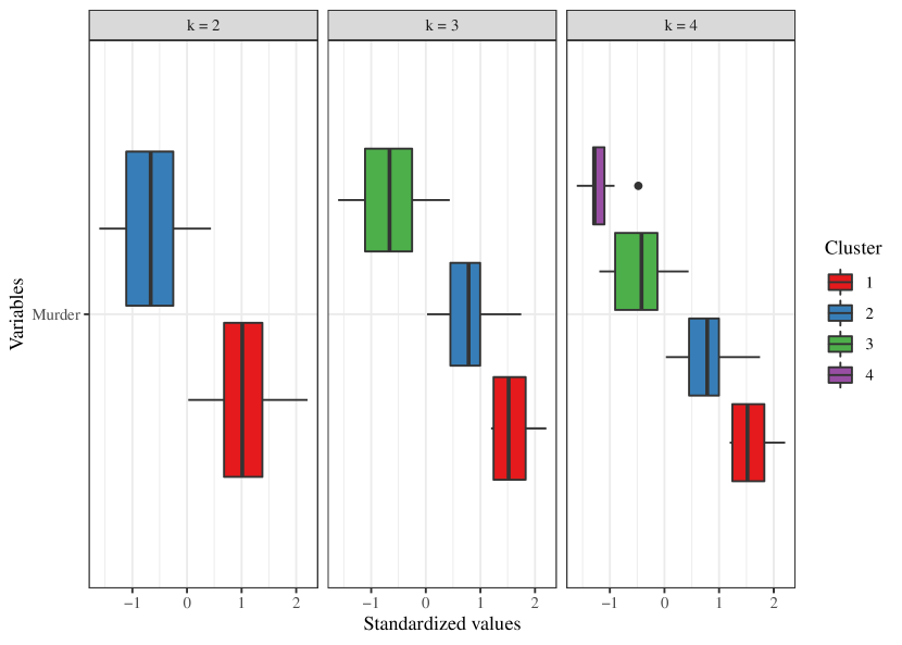
Figure 10: Boxplots with different segmentation

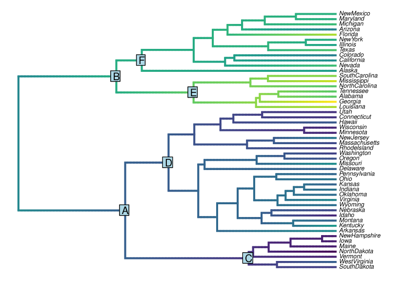
Figure 11: Murder evolutionary dendrogram

Figure 12: Comparisson between the boxplot visualization and the evolutionary dendrogram on the murder feature from the USArrests dataset. Evolutionary dendrograms provide more nuanced information as they take the full dendrogram hierarchy into account.

Figure 10 presents boxplots grouped by cluster when $2$, $3$ and $4$ clusters are used. Using these plots, one can see that the feature is well segmented for the chosen number of clusters. However, although boxplots bring measures of centrality and dispersion, they lose information about the internal structure of each cluster. In particular, one cannot find in the boxplots which instances belong to each cluster.

In contrast Figure 11 displays the evolutionary dendrogram obtained for the same feature. By cutting the dendrogram at the root, one obtains the main top (B: green) and bottom (A: light blue) clusters. By looking at the color dispersion in both clusters, it is possible to conclude that the top cluster has a larger variance than the bottom cluster. Furthermore, by looking at the next internal nodes, one can observe that while the top cluster can be further segmented into dark green (F) and light green (E) sub-clusters, the bottom cluster can be segmented into purple (C) and dark blue (D) sub-clusters.

5.2 PFIS vs. state-of-the-art importance scores

This subsection compares PFIS, presented in subsection 3.3, to common alternatives for assessing feature importance in a dendrogram. We use the following baselines:

• [Classification-based importance - RF (Badih et al.,, 2019; Ismaili et al.,, 2014)]. We first cut the dendrogram into $k$ clusters. Next, these clusters are used as labels for a random forest classifier (Breiman,, 2001) that uses the original features as inputs. Finally, the importance scores infered by the random forest are used as the importance of the features for the dendrogram.

• [Classification-based importance - XGBoost (Badih et al.,, 2019; Ismaili et al.,, 2014)]. Same as before, but using a XGboost classifier (Chen and Guestrin,, 2016) instead.

• [LOVO (Badih et al.,, 2019)]. A leave-one-variable-out (LOVO) approach that compares within–cluster heterogeneity by ommiting each feature from the dataset. This approach also requires the dendrogram to be cut into $k$ clusters.

In order to compare the performance of these approaches to PFIS, we need a dataset in which the ground-truth importance is know. Thus, we simulated data in a way that allows the true importance to be evaluated. Specifically, let $X_{i,j}$ be the $j$-th simulated feature value of the $i$-th instance, where $1\leq j\leq 6$ and $1\leq i\leq 2^{8}$. The data, $X$, is generated recursively according to a tree procedure described in Algorithm 2. In this algorithm, $\theta_{i,j,k-1}$ represents an ancestor of $\theta_{i,j,k}$ and of $\theta_{2^{k-1}+i,j,k}$. Also, $z_{i,j,k}$ represents the noise that is added when generating a descendant. Algorithm 2 summarizes this procedure. Observe that $z_{i,j,k}$ is of the order of magnitude of $(\sigma_{j})^{k}$. That is, the larger the value of $\sigma_{j}$, the more noise is added to the leaf descendants proportionally to the internal nodes of the tree. As a result, the larger the value of $\sigma_{j}$, the less the structure of the tree is preserved by feature $j$. Since in the simulation $\sigma_{j}=2^{j-3}$, one expects that the feature importance in the adjusted dendrogram should decrease from $j=1$ to $6$.

Algorithm 2 Simulated data to compare feature importance methods

Output: $X_{i,j}$, the simulated data.

1:Let $\sigma=(2^{-2},2^{-1},2^{0},2^{1},2^{2},2^{3})$.

2:Let $\theta_{1,j,0}=0$, for $1\leq j\leq 6$.

3:for each $k\in\{1,\ldots,7\}$, do

4:     for each $i\in\{1,\ldots,2^{k-1}\}$ and $j\in\{1\ldots,6\}$, do

5:         Let $i_{1}=i$ and $i_{2}=2^{k-1}+i$

6:         Let $\theta_{i_{1},j,k}=\theta_{i_{1},j,k-1}+z_{i_{1},j,k}$, where $z_{i_{1},j,k}\sim N(0,(\sigma_{j})^{k})$

7:         Let $\theta_{i_{2},j,k}=\theta_{i_{1},j,k-1}+z_{i_{2},j,k}$, where $z_{i_{1},j,k}\sim N(0,(\sigma_{j})^{k})$

8:     end for

9:end for

10:Let $X_{i,j}=\theta_{i,j,7}$, for $1\leq i\leq 2^{8}$ and $1\leq j\leq 6$.

Figure 13 shows the various importance scores to the data described above. The dendrogram was obtained through Ward’s method, and the scores that required a fixed number of clusters used $k=3$ groups, which is the optimal number of clusters according to the NbClust majority rule (Charrad et al.,, 2014). The right panel presents $\sigma_{j}^{-1}$, a measure of how much the tree structure is preserved by each feature. The figure shows that our method (PFIS) is the only one to preserve the ordering of the features given by $\sigma_{j}^{-1}$, and thus uncover the true feature importance values.

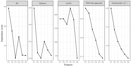
Figure 13: Measures of feature importance: (far left) random forest (Ismaili et al.,, 2014), (middle left) XGboost (Ismaili et al.,, 2014), (middle) leave-one-variable-out (Badih et al.,, 2019), (middle right) PFIS, (far right) $\sigma_{j}^{-1}$, a gold standard (ground truth) that measures how much the tree structure that is used to generate the data is preserved by each feature. Our score preserves the ordering given by $\sigma_{j}^{-1}$, while all the others do not.

5.3 Cross-validated Loss vs. state-of-the-art dendrogram selection tools

We use simulated and real data to compare our CVL loss to other state-of-the-art dendrogram selection tools. For each experiment we will use different combinations of clustering methods and linkages in order to assess the quality and performance of each methodology. The combinations of methods and linkages are listed in Table 1.

This section evaluates the performance of cross-validated loss ($CVL$) by comparing it to the following baselines:

• [Cophenetic Correlation score - COPH (Sokal and Rohlf,, 1962; Timofeeva,, 2019; Saraçli et al.,, 2013)]. The idea of the cophenetic correlation is to compute the pearson correlation between the euclidean distance and the dendrogrammatic (or cophenetic) distance obtained for each different pair of observations. The dendrogrammatic distance is given by the height of the node of the obtained dendrogram at which each pair of observations are first joined together.

• [Figure of Merit - FOM (Yeung et al.,, 2001)]. First, for each feature, a dendrogram is adjusted holding out the feature from the data. Next, by cutting each dendrogram at a given height, it is transformed into a partition. Finally, the within-cluster similarity is computed for each held-out feature using its respective partition. The FOM score corresponds to the average of these similarities.

• [Adjusted Rand Index - ARI (Hubert and Arabie,, 1985)]. The standard rand index (Rand,, 1971) measures the similarity between a clustering of the data and a ground truth label by considering all pairs of observations and counting the pairs that are assigned to the same cluster. ARI adds a correction to the rand index that takes into account assignment to the same clustering by chance.

Table 1: Clustering methods used for comparing CVL to FOM, COPH and ARI.

Method	Linkages
Agnes	weighted, average and ward
Agglomerative	ward.D, complete, single, ward.D2,
	average, mcquitty and median
Diana	Not applicable

We compare CVL to these scores using simulated datasets and UCI datasets that are available on $R$. The chosen UCI datasets are summarized in Table 2. We also use a simulated dataset with $250$ instances such that the label is $Y_{i}\sim\text{Bernoulli}(0.5)$ and the features are $(X_{1},X_{2})|Y\sim\text{N}_{2}(\begin{bmatrix}2Y&2Y\end{bmatrix},\boldsymbol{I})$. Note that although clustering methods use only features, each dataset also has a label.

Table 2: Datasets from UCI used to compare CVL to FOM.

Dataset	Sample size	Number of features	Label
Simulated	250	2	$Y$
Iris	150	4	Species
Diabetes	768	8	$V9$
Wheat seeds	210	7	$V8$
Ionosphere	351	34	label
Glass	214	10	$V11$
Haberman	306	3	$V4$
Wine	178	13	$V1$

We compare all methods to a gold-standard which uses the labels in the datasets. The main idea is that the dendrogram is treated as a classifier for the label and the F1 score is the gold-standard for the dendrogram’s performance. Such a classifier is obtained by cutting the dendrogram at an appropriate height so that it becomes a partition with size equal to the number of labels. Next, each cluster in the partition is associated to a single label that maximizes accuracy. Each instance is labeled equally as the partition to which it belongs. The gold-standard for the dendrogram’s performance is the F1 score based on its assigned labels.

Based on the above information, it is possible to describe the experiment that compares CVL, FOM, Cophenetic correlation and ARI. For each dataset, we performed clustering using all of the the methods in Table 1. Each of the $11$ clustering methods was applied using the euclidean, manhattan and canberra distances. As a result, $33$ dendrograms were obtained for each dataset. For each dendrogram, the CVL, FOM, COPH, ARI and gold-standard F1 scores were calculated. Since FOM and ARI require a pre-defined number of clusters, we calculated both scores using the correct number of labels. Since the correct number of clusters is generally unavailable, this procedure gives an advantage to FOM and ARI.

Table 3 shows, for each dataset, the Spearman correlation between $CVL$ and $F1$, $FOM$ and $F1$, $-COPH$ and $F1$ and between $-ARI$ and $F1$ among the clustering methods that were used. Recall that, while CVL and FOM measure how bad is a given clustering, the gold standard $F1$ and the scores $ARI$ and $COPH$ are methods that measure whether the clustering is good. Therefore, a negative correlation between a loss or minus a score and F1 indicates that the measures are in agreement. One can observe in Table 3 that, while the Spearman correlation between CVL and F1 and -COPH and F1 is negative for all but one dataset, it is positive between FOM and F1 and $-ARI$ and F1 except for two and five datasets respectively. Furthermore, both CVL and COPH outperformed the other methods in three out of the eight datasets each, while ARI performed better for two datasets. Thus, these results provide evidence that both the cophenetic correlation and CVL adequately assess the performance of clustering methods without the need to partition the dendrogram. In practice, they can complement each other to perform dendrogram selection.

Table 3: For each dataset, Spearman correlation between CVL and F1, CVL and FOM , COPH and F1 and ARI and F1 among the $33$ clustering methods used in the experiment. In order to maintain the comparison sign for all losses/scores, we compared minus the value of COPH and ARI to F1, as indicated by the sign in front of both scores. Bold values indicate which of the losses/scores has the lowest correlation with $F_{1}$ and, therefore, is in better agreement with this performance measure.

	Correlations
Dataset	$CVL({\mathcal{T}})$ vs $F_{1}$	$FOM$ vs $F_{1}$	$-COPH$ vs $F_{1}$	$-ARIvsF_{1}$
Simulated	-0.40	0.23	-0.23	0.88
Iris	0.26	0.10	-0.54	-0.30
Pima indians	-0.53	0.52	-0.63	-0.06
Wheat seeds	-0.11	-0.48	0.28	-0.83
Ionosphere	-0.43	0.63	-0.12	0.60
Glass	-0.15	0.19	-0.48	0.14
Haberman	-0.42	0.38	-0.16	-0.09
Wine	-0.21	-0.84	-0.35	-0.92

References

- Badih et al., (2019) Badih, G., Pierre, M., and Laurent, B. (2019). Assessing variable importance in clustering: a new method based on unsupervised binary decision trees. Computational Statistics, 34:301–321.
- Bollback, (2006) Bollback, J. P. (2006). SIMMAP: stochastic character mapping of discrete traits on phylogenies. BMC bioinformatics, 7(1):88.
- Borges et al., (2021) Borges, L. M., Izbicki, R., and Stern, R. B. (2021). The overlooked role of predictiveness in phylogenetics: Data-splitting as a powerful method for model selection. submitted.
- Breiman, (2001) Breiman, L. (2001). Random forests. Machine learning, 45(1):5–32.
- Caliński and Harabasz, (1974) Caliński, T. and Harabasz, J. (1974). A dendrite method for cluster analysis. Communications in Statistics-theory and Methods, 3:1–27.
- Charrad et al., (2014) Charrad, M., Ghazzali, N., Boiteau, V., and Niknafs, A. (2014). Nbclust: an r package for determining the relevant number of clusters in a data set. Journal of statistical software, 61:1–36.
- Chen and Guestrin, (2016) Chen, T. and Guestrin, C. (2016). Xgboost: A scalable tree boosting system. In Proceedings of the 22nd acm sigkdd international conference on knowledge discovery and data mining, pages 785–794.
- Chen et al., (2014) Chen, Y., Kim, J., and Mahmassani, H. (2014). Pattern recognition using clustering algorithm for scenario definition in traffic simulation-based decision support systems.
- Clavel et al., (2015) Clavel, J., Escarguel, G., and Merceron, G. (2015). mvmorph: an r package for fitting multivariate evolutionary models to morphometric data. Methods in Ecology and Evolution, 6(11):1311–1319.
- Coscrato et al., (2019) Coscrato, V., Inácio, M. H. d. A., Botari, T., and Izbicki, R. (2019). Nls: an accurate and yet easy-to-interpret regression method. arXiv preprint arXiv:1910.05206.
- Datta and Datta, (2003) Datta, S. and Datta, S. (2003). Comparisons and validation of statistical clustering techniques for microarray gene expression data. Bioinformatics, 19(4):459–466.
- Felsenstein, (1985) Felsenstein, J. (1985). Phylogenies and the comparative method. The American Naturalist, 125(1):1–15.
- Fisher, (1936) Fisher, R. A. (1936). The use of multiple measurements in taxonomic problems. Annals of eugenics, 7(2):179–188.
- Fukunaga and Hostetler, (1975) Fukunaga, K. and Hostetler, L. (1975). The estimation of the gradient of a density function, with applications in pattern recognition. IEEE Transactions on Information Theory, 21(1):32–40.
- Galili, (2015) Galili, T. (2015). dendextend: an R package for visualizing, adjusting and comparing trees of hierarchical clustering. Bioinformatics, 31(22):3718–3720.
- Hair, (2009) Hair, J. F. (2009). Multivariate data analysis.
- (17) Hastie, T., Tibshirani, R., and Friedman, J. (2009a). The Elements of Statistical Learning: Data Mining, Inference, and Prediction, Second Edition. Springer Series in Statistics. Springer New York.
- (18) Hastie, T., Tibshirani, R., Friedman, J. H., and Friedman, J. H. (2009b). The elements of statistical learning: data mining, inference, and prediction, volume 2. Springer.
- Hennig, (2015) Hennig, C. (2015). Clustering strategy and method selection. Handbook of cluster analysis, 9:703–730.
- Hubert and Arabie, (1985) Hubert, L. and Arabie, P. (1985). Comparing partitions. Journal of classification, 2:193–218.
- Ismaili et al., (2014) Ismaili, O. A., Lemaire, V., and Cornuéjols, A. (2014). A supervised methodology to measure the variables contribution to a clustering. In Loo, C. K., Yap, K. S., Wong, K. W., Teoh, A., and Huang, K., editors, Neural Information Processing, pages 159–166, Cham. Springer International Publishing.
- Izbicki and Lee, (2017) Izbicki, R. and Lee, A. B. (2017). Converting high-dimensional regression to high-dimensional conditional density estimation. Electronic Journal of Statistics, 11(2):2800–2831.
- James et al., (2013) James, G., Witten, D., Hastie, T., and Tibshirani, R. (2013). An introduction to statistical learning, volume 112. Springer.
- Jardine and van Rijsbergen, (1971) Jardine, N. and van Rijsbergen, C. (1971). The use of hierarchic clustering in information retrieval. Information Storage and Retrieval, 7(5):217 – 240.
- Joy et al., (2016) Joy, J. B., Liang, R. H., McCloskey, R. M., Nguyen, T., and Poon, A. F. (2016). Ancestral reconstruction. PLoS computational biology, 12(7):e1004763.
- Kassambara, (2017) Kassambara, A. (2017). Practical guide to cluster analysis in R: Unsupervised machine learning, volume 1. Sthda.
- Liu et al., (2006) Liu, J., Bai, Y., Kang, J., and An, N. (2006). A new approach to hierarchical clustering using partial least squares. In 2006 International Conference on Machine Learning and Cybernetics, pages 1125–1131.
- MacQueen, (1967) MacQueen, J. (1967). Some methods for classification and analysis of multivariate observations. In Proceedings of the Fifth Berkeley Symposium on Mathematical Statistics and Probability, Volume 1: Statistics, pages 281–297, Berkeley, Calif. University of California Press.
- McNeil, (1977) McNeil, D. R. (1977). Interactive data analysis: a practical primer.
- Neter et al., (1996) Neter, J., Kutner, M. H., Nachtsheim, C. J., Wasserman, W., et al. (1996). Applied linear statistical models.
- O’Meara et al., (2006) O’Meara, B. C., Ané, C., Sanderson, M. J., and Wainwright, P. C. (2006). Testing for different rates of continuous trait evolution using likelihood. Evolution, 60(5):922–933.
- Paradis and Schliep, (2019) Paradis, E. and Schliep, K. (2019). ape 5.0: an environment for modern phylogenetics and evolutionary analyses in r. Bioinformatics, 35(3):526–528.
- Pfaffel, (2021) Pfaffel, O. (2021). FeatureImpCluster: Feature Importance for Partitional Clustering. R package version 0.1.5.
- Pupko and Mayrose, (2020) Pupko, T. and Mayrose, I. (2020). A gentle introduction to probabilistic evolutionary models.
- Rand, (1971) Rand, W. M. (1971). Objective criteria for the evaluation of clustering methods. Journal of the American Statistical association, 66(336):846–850.
- Revell, (2012) Revell, L. J. (2012). phytools: an r package for phylogenetic comparative biology (and other things). Methods in ecology and evolution, 3(2):217–223.
- Revell, (2013) Revell, L. J. (2013). Two new graphical methods for mapping trait evolution on phylogenies. Methods in Ecology and Evolution, 4(8):754–759.
- Rocha et al., (2009) Rocha, L. M., Cappabianco, F. A. M., and Falcão, A. X. (2009). Data clustering as an optimum-path forest problem with applications in image analysis. International Journal of Imaging Systems and Technology, 19(2):50–68.
- Rosenberg and Hirschberg, (2007) Rosenberg, A. and Hirschberg, J. (2007). V-measure: A conditional entropy-based external cluster evaluation measure. pages 410–420.
- Rousseeuw, (1987) Rousseeuw, P. J. (1987). Silhouettes: a graphical aid to the interpretation and validation of cluster analysis. Computational and Applied Mathematics, 20:53–65.
- Rousseeuw and Kaufman, (1990) Rousseeuw, P. J. and Kaufman, L. (1990). Finding groups in data. Hoboken: Wiley Online Library, 1.
- Saraçli et al., (2013) Saraçli, S., Doğan, N., and Doğan, İ. (2013). Comparison of hierarchical cluster analysis methods by cophenetic correlation. Journal of inequalities and Applications, 2013(1):1–8.
- Seo and Shneiderman, (2002) Seo, J. and Shneiderman, B. (2002). Interactively exploring hierarchical clustering results [gene identification]. Computer, 35(7):80–86.
- Shimizu et al., (2022) Shimizu, G. Y., Izbicki, R., and de Carvalho, A. C. (2022). Model interpretation using improved local regression with variable importance. arXiv preprint arXiv:2209.05371.
- Sokal and Rohlf, (1962) Sokal, R. R. and Rohlf, F. J. (1962). The comparison of dendrograms by objective methods. Taxon, pages 33–40.
- Tibshirani, (1996) Tibshirani, R. (1996). Regression shrinkage and selection via the lasso. Journal of the Royal Statistical Society: Series B (Methodological), 58(1):267–288.
- Timofeeva, (2019) Timofeeva, A. (2019). Evaluating the robustness of goodness-of-fit measures for hierarchical clustering. In Journal of Physics: Conference Series, volume 1145, page 012049. IOP Publishing.
- Van der Maaten and Hinton, (2008) Van der Maaten, L. and Hinton, G. (2008). Visualizing data using t-sne. Journal of machine learning research, 9(11).
- Vendramin et al., (2010) Vendramin, L., Campello, R. J., and Hruschka, E. R. (2010). Relative clustering validity criteria: A comparative overview. Statistical analysis and data mining: the ASA data science journal, 3(4):209–235.
- Ward Jr, (1963) Ward Jr, J. H. (1963). Hierarchical grouping to optimize an objective function. Journal of the American statistical association, 58(301):236–244.
- Yeung et al., (2001) Yeung, K. Y., Haynor, D. R., and Ruzzo, W. L. (2001). Validating clustering for gene expression data. Bioinformatics, 17(4):309–318.
- Zhu, (2018) Zhu, X. (2018). Variable diagnostics in model-based clustering through variation partition. Journal of Applied Statistics, 45(16):2888–2905.