Sample Prior Guided Robust Model Learning to Suppress Noisy Labels

Abstract

Imperfect labels are ubiquitous in real-world datasets and seriously harm the model performance. Several recent effective methods for handling noisy labels have two key steps: 1) dividing samples into cleanly labeled and wrongly labeled sets by training loss, 2) using semi-supervised methods to generate pseudo-labels for samples in the wrongly labeled set. However, current methods always hurt the informative hard samples due to the similar loss distribution between the hard samples and the noisy ones. In this paper, we proposed PGDF (Prior Guided Denoising Framework), a novel framework to learn a deep model to suppress noise by generating the samples’ prior knowledge, which is integrated into both dividing samples step and semi-supervised step. Our framework can save more informative hard clean samples into the cleanly labeled set. Besides, our framework also promotes the quality of pseudo-labels during the semi-supervised step by suppressing the noise in the current pseudo-labels generating scheme. To further enhance the hard samples, we reweight the samples in the cleanly labeled set during training. We evaluated our method using synthetic datasets based on CIFAR-10 and CIFAR-100, as well as on the real-world datasets WebVision and Clothing1M. The results demonstrate substantial improvements over state-of-the-art methods.

Introduction

Deep learning techniques, such as convolutional neural networks (CNNs) and recurrent neural networks (RNNs), have recently achieved great success in object recognition (Montserrat et al. 2017), image classification (Krizhevsky, Sutskever, and Hinton 2012), and natural language processing (NLP) (Young et al. 2018). Most existing CNN or RNN deep models mainly rely on collecting large scale labeled datasets, such as ImageNet (Russakovsky et al. 2015). However, it is very expensive and difficult to collect a large scale dataset with clean labels (Yi and Wu 2019). Moreover, in the real world, noisy labels are often inevitable in manual annotation (Sun et al. 2019). Therefore, research on designing robust algorithms with noisy labels is of great significance (Wei et al. 2019).

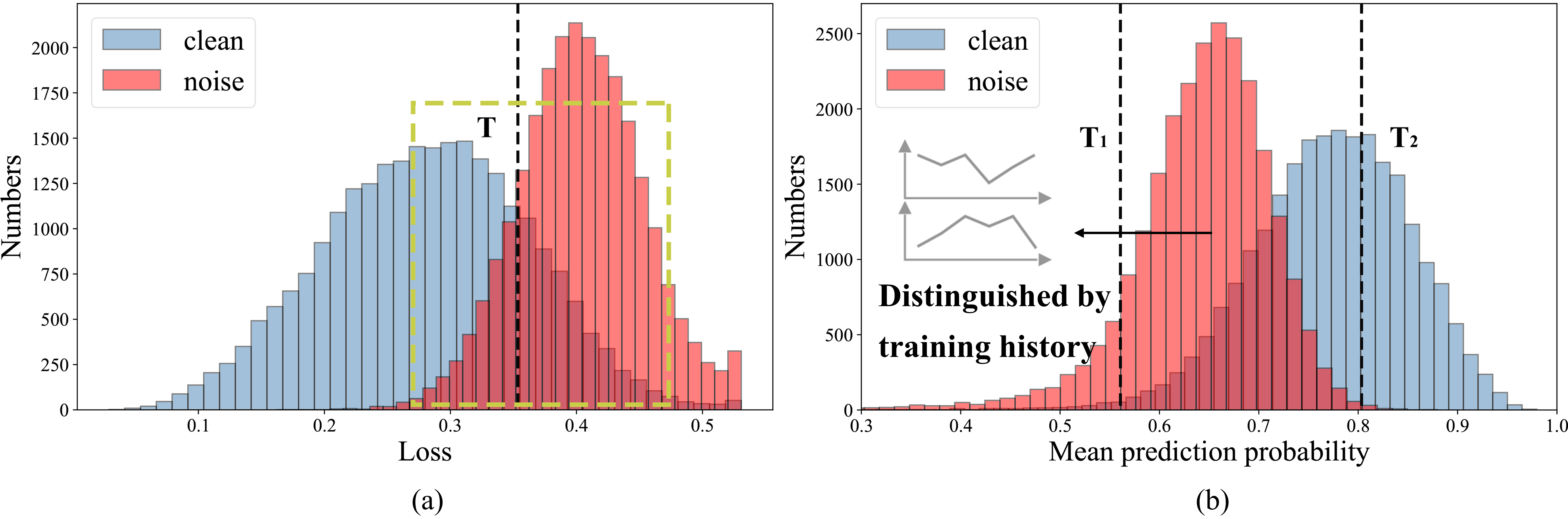
Figure 1: (a) Loss distribution of the clean and noise samples in CIFAR-100 with 50% symmetric noise ratio. (b) Mean prediction probability distribution of the clean and noisy samples in CIFAR-100 with 50% symmetric noise ratio.

In the literature, a lot of approaches were proposed to improve the learning performance with label noise, such as estimating the noise transition matrix (Goldberger and Ben-Reuven 2017; Patrini et al. 2017), designing noise-robust loss functions (Ghosh, Kumar, and Sastry 2017; Lyu and Tsang 2019; Xu et al. 2019), designing noise-robust regularization (Liu et al. 2020; Tanno et al. 2020), sample selection (Han et al. 2018; Chen et al. 2019), and semi-supervised learning (Li, Socher, and Hoi 2020; Cordeiro et al. 2021). Recently, methods of semi-supervised learning achieve state-of-the-art performance. They always first divide samples into cleanly labeled and wrongly labeled sets by training loss, and then use semi-supervised methods to generate pseudo-labels for samples in the wrongly labeled set. The sample dividing step is generally based on the small-loss strategy (Yu et al. 2019), where at every epoch, samples with small loss are classified as clean data, and large loss as noise. However, the above methods fail in distinguishing informative hard samples from noisy ones due to their similar loss distributions (as depicted in Figure 1(a), samples in the yellow dotted box are indistinguishable), and thus may neglect the important information of the hard samples (Xiao et al. 2015). To the best of our knowledge, there are very few works studying hard samples under noisy label scenarios. Work (Wang et al. 2019) mentioned the hard samples in learning with noisy labels, but that work did not explicitly identify hard samples.

Although the hard samples and noisy samples cannot be directly distinguished by training loss, we observed that they have different behaviors in training history. Through this intuition, we propose PGDF (Prior Guided Denoising Framework), a novel framework to learn a deep model to suppress noise. We first use the training history to distinguish the hard samples from the noisy ones (as depicted in Figure 1(b), samples between two thresholds are distinguished by training history). Thus, we classify the samples into three sets by using the prior knowledge. The divided dataset is then guiding the subsequent training process. Our key findings and contributions are summarized as follows:

• Hard samples and noisy samples can be recognized using training history. We first propose a Prior Generation Module, which generates the prior knowledge to pre-classify the samples into an easy set, a hard set, and a noisy set. We further optimize the pre-classification result at each epoch with adaptive sample attribution obtained by Gaussian Mixture Model.

• We realize robust noisy labels suppression based on the divided sets. On one hand, we generate high-quality pseudo-labels by the estimated distribution transition matrix with the divided easy set. On the other hand, we further safely enhance the informative samples in the hard set, while previous existing noisy labels processing methods cannot achieve this because they fail to distinguish the hard samples and noisy ones.

• We experimentally show that our PGDF significantly advances state-of-the-art results on multiple benchmarks with different types and levels of label noise. We also provide the ablation study to examine the effect of different components.

Related Work

In this section we describe existing works on learning with noisy labels. Typically, the noisy-label processing algorithms can be classified into five categories by exploring different strategies: estimating the noise transition matrix (Goldberger and Ben-Reuven 2017; Patrini et al. 2017), designing noise-robust loss functions (Ghosh, Kumar, and Sastry 2017; Lyu and Tsang 2019; Xu et al. 2019; Zhou et al. 2021a, b), adding noise-robust regularization (Liu et al. 2020; Tanno et al. 2020), selecting sample subset (Han et al. 2018; Chen et al. 2019; Huang et al. 2019), and semi-supervised learning (Li, Socher, and Hoi 2020; Cordeiro et al. 2021).

In the first category, different transition matrix estimation methods were proposed in (Goldberger and Ben-Reuven 2017; Patrini et al. 2017), such as using additional softmax layer (Goldberger and Ben-Reuven 2017), and two-step estimating scheme (Patrini et al. 2017). However, these transition matrix estimations fail in real-world datasets where the utilized prior assumption is no longer valid (Han, Luo, and Wang 2019). Being free of transition matrix estimation, the second category targets at designing loss functions that have more noise-tolerant power. Work in (Ghosh, Kumar, and Sastry 2017) adopted mean absolute error (MAE) which demonstrates more noise-robust ability than cross-entropy loss. The authors in work (Xu et al. 2019) proposed determinant-based mutual information loss which can be applied to any existing classification neural networks regardless of the noise pattern. Recently, work (Zhou et al. 2021b) proposed a novel strategy to restrict the model output and thus made any loss robust to noisy labels. Nevertheless, it has been reported that performances with such losses are significantly affected by noisy labels (Ren et al. 2018). Such implementations perform well only in simple cases where learning is easy or the number of classes is small. For designing noise-robust regularization, work in (Tanno et al. 2020) assumed the existence of multiple annotators and introduced a regularized EM-based approach to model the label transition probability. In work (Liu et al. 2020), a regularization term was proposed to implicitly prevent memorization of the false labels.

Most recent successful sample selection strategies in the fourth category conducted noisy label processing by selecting clean samples through ”small-loss” strategy. Work (Jiang et al. 2018) pre-trained an extra network, and then used the extra network for selecting clean instances to guide the training. The authors in work (Han et al. 2018) proposed a Co-teaching scheme with two models, where each model selected a certain number of small-loss samples and fed them to its peer model for further training. Based on this scheme, work (Chen et al. 2019) tried to improve the performance by proposing an Iterative Noisy Cross-Validation (INCV) method. Work (Huang et al. 2019) adjusted the hyper-parameters of model to make its status transfer from overfitting to underfitting cyclically, and recorded the history of sample training loss to select clean samples. This family of methods effectively avoids the risk of false correction by simply excluding unreliable samples. However, they may eliminate numerous useful samples. To solve this shortcoming, the methods of the fifth category based on semi-supervised learning treated the noisy samples as unlabeled samples, and used the outputs of classification models as pseudo-labels for subsequent loss calculations. The authors in (Li, Socher, and Hoi 2020) proposed DivideMix, which relied on MixMatch (Berthelot et al. 2019) to linearly combine training samples classified as clean or noisy. Work (Cordeiro et al. 2021) designed a two-stage method called LongReMix, which first found the high confidence samples and then used the high confidence samples to update the predicted clean set and trained the model. Recently, work (Nishi et al. 2021) used different data augmentation strategies in different steps to improve the performance of DivideMix, and work (Zheltonozhskii et al. 2022) used a self-supervised pre-training method to improve the performance of DivideMix.

The above sample selection strategy and semi-supervised learning strategy both select the samples with clean labels for the subsequent training process. All of their selecting strategies are based on the training loss because the clean samples tend to have small loss during training. However, they will hurt the informative hard samples due to the similar loss distribution between the hard samples and the noisy ones. Our work strives to reconcile this gap by distinguishing the hard samples from the noisy ones by introducing a sample prior.

Method

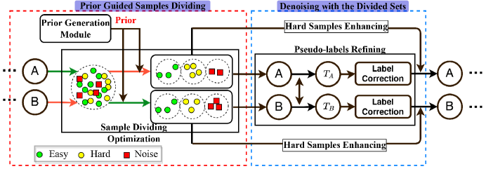
Figure 2: PGDF first generates the prior knowledge by the Prior Generation Module. Then, it trains two models (A and B) simultaneously. At each epoch, a model divides the original dataset into an easy set, a hard set, and a noisy set by combining the prior knowledge and the loss value of each sample. The divided dataset is used by the other network. After the first stage, the models conduct label correction for samples with the help of the estimated distribution transition matrix. Finally, the training loss is reweighted by the dividing result to further enhance the hard samples.

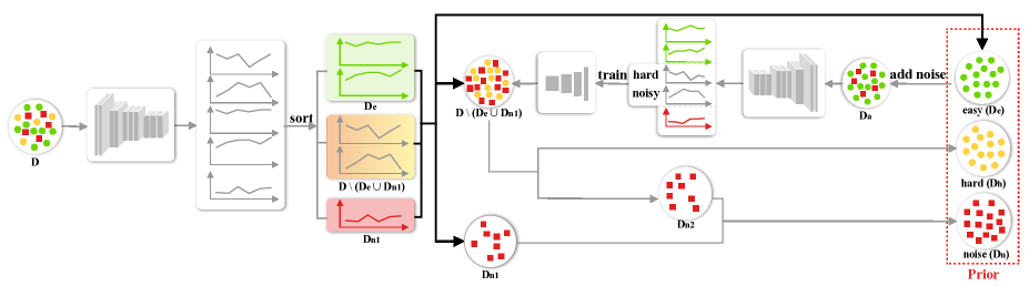
Figure 3: The overview of the Prior Generation Module. It pre-classifies the samples into an easy set, a hard set, and a noisy set.

The overview of our proposed PGDF is shown in Figure 2. The first stage (Prior Guided Sample Dividing) of PGDF is dividing the samples into an easy set, a hard set, and a noisy set. The Prior Generation Module first pre-classifies the samples into three sets as prior knowledge; then, at each epoch, the pre-classification result is optimized by the training loss (Sample Dividing Optimization). With the divided sets, the second stage (Denoising with the Divided Sets) conducts label correction for samples with the help of the estimated distribution transition matrix (Pseudo-labels Refining), and then the hard samples are further enhanced (Hard Samples Enhancing). The details of each component are described in the following.

Prior Guided Sample Dividing

Algorithm 1 Prior Generation Module.

0:  $D=[d_{1},d_{2},...,d_{n}]$, $d_{i}$ is input image, label $Y=[y_{1},y_{2},...,y_{n}]$, $y_{i}$ is label for $d_{i}$, easy samples ratio $\tau_{e}$, part of noisy samples ratio $\tau_{n1}$

0:  easy set $D_{e}$, hard set $D_{h}$, noise set $D_{n}$

1:  Train classification model $M_{c}$ by using $D$ and $Y$, record training history $H=[h_{1},h_{2},...,h_{n}]$, where $h_{i}$ is a vector with shape of $1*k(epoch)$

2:  Calculate the mean value of $H$ as $H_{m}$, $H_{m}=[mean(h_{1}),mean(h_{2}),...,mean(h_{n})]$, sort $D$ descending by $H_{m}$, select easy samples $D_{e}=D[0:len(D)*\tau_{e}]$, select part of noisy samples $D_{n1}=D[len(D)*(1-\tau_{n1}):len(D)]$

3:  Add noise to $D_{e}$ as $D_{a}$, get noisy label $Y_{n}$ and record whether it is noise or not $R=[r_{1},r_{2},...,r_{n}]$

4:  Retrain $M_{c}$ by $D_{a}$ and $Y_{n}$, record training history $H_{n}$

5:  Sort $H_{n}$ descending by mean, select training history $H_{n}’=H_{n}[len(H_{n})*\tau_{e}:len(H_{n})*(1-\tau_{n1})]$

6:  Train classifier $M_{m}$ by using $H_{n}^{\prime}$ and $R$

7:  Put the samples in $D\setminus(D_{e}\cup D_{n1})$ into $M_{m}$ and get $D_{h}$ and $D_{n2}$

8:  $D_{n}=D_{n1}\cup D_{n2}$

9:  return $D_{e}$, $D_{h}$, $D_{n}$

Prior Generation Module. Previous work (Zhang et al. 2016) shows that CNNs tend to memorize simple samples first, and then the networks can gradually learn all the remaining samples, even including the noisy samples, due to the high representation capacity. According to this finding, many methods use the “small-loss” strategy, where at each epoch, samples with small loss are classified as clean data and large loss as noise. Sample with small loss means the prediction probability of the model output is closer to the supervising label. We directly used the normalized probability for analysis since the loss value is just calculated by the normalized probability and the ground truth label. We first train a CNN classification model with the data, and record the probability history of the model output for each sample on the class of its corresponding label. Then, we calculate the mean prediction probability value of the sample training history which is shown in Figure 1(b). The figure shows the clean sample tends to have a higher mean prediction probability than the noisy one. Therefore, we can set two thresholds (such as the black dotted lines in Figure 1(b)). Samples with mean prediction probability lower than $T_{1}$ are almost noisy, while higher than $T_{2}$ are almost clean. However, we still cannot distinguish the samples with mean prediction probability between two thresholds. We define this part of clean data as hard samples in our work.

In order to distinguish the hard samples from the noisy ones, we construct the Prior Generation Module based on the prediction history of the training samples, as depicted by Figure 3. For the training set $D$ with $N$ samples, we gradually obtain the corresponding $N$ prediction probability maps through the training of a CNN classification model for $k$ epochs. This module first selects easy samples $D_{e}$ and part of noisy samples $D_{n1}$ by using the mean prediction probability values. Then we manually add noise to the $D_{e}$ as $D_{a}$ and record whether the sample is noise or not. The noise ratio of the adding noise is the same as the original dataset, which can be known or estimated by the noise cross-validation algorithm of work (Chen et al. 2019). After that, we train the same classification model by using $D_{a}$ and record training history again. Then we discard the “easy samples” and part of “noisy samples” of $D_{a}$ according to mean prediction probability, and utilize the rest samples as training data to train the classifier. We use a simple one dimension CNN which contains 3 one dimension convolution layers and a fully connected layer as the classifier here. So far, we will obtain a classifier that takes the prediction probability map of training history as input, and output whether it is a hard sample or a noisy one. Finally, we put the samples in $D\setminus(D_{e}\cup D_{n1})$ into the classifier to get the hard sample set $D_{h}$ and a part of the noisy set $D_{n2}$, and we combine $D_{n1}$ and $D_{n2}$ as the noisy set $D_{n}$. Algorithm 1 shows the details of this module.

Sample Dividing Optimization. Considering the online training loss at each epoch is also important information to help sample dividing, we apply this information to optimize the pre-classification result. Specifically, as shown in Figure 2, at each epoch, we get the clean probability $w_{it}$ of each sample from training loss by using Gaussian Mixture Model (GMM) following previous work (Li, Socher, and Hoi 2020). And we have already got the prior knowledge of each sample, we set the clean probability of prior knowledge as $w_{ip}$ from Equation (1),

$$w_{ip}=\left\{\begin{array}[]{cc}1,&d_{i}\in D_{e}\\ p_{h},&d_{i}\in D_{h}\\ 1-p_{n},&d_{i}\in D_{n_{2}}\\ 0,&d_{i}\in D_{n_{1}}\end{array}\right.,$$ (1)

where $p_{h}$ is the classifier ($M_{m}$) prediction probability for $d_{i}$ to be hard sample and $p_{n}$ is the classifier prediction probability for $d_{i}$ to be noisy sample. Then, we combine $w_{it}$ and $w_{ip}$ to get the clean probability $w_{i}$ by Equation (2),

$$w_{i}=\left\{\begin{array}[]{cc}1,&d_{i}\in D_{e}\\ mw_{it}+(1-m)w_{ip},&d_{i}\in D_{h}\cup D_{n}\end{array}\right.,$$ (2)

where $m$ is a hyper-parameter. Finally, we divide samples with $w_{i}$ equal to $1$ into the easy set $\tilde{D_{e}}$, the samples with $0.5<w_{i}<1$ are divided into the hard set $\tilde{D_{h}}$, and the rest samples are divided into the noisy set $\tilde{D_{n}}$. Each network divides the original dataset for the other network to use to avoid confirmation bias of self-training similar to previous works (Han et al. 2018; Chen et al. 2019; Li, Socher, and Hoi 2020).

Denoising with the Divided Sets

Pseudo-labels Refining. After the sample dividing phase, we combine the outputs of the two models to generate the pseudo-labels $P$ to conduct label correction, similar to “co-guessing” in DivideMix (Li, Socher, and Hoi 2020). Considering the samples in the easy set are highly reliable, we can use this part of data to estimate the distribution difference between pseudo-label and the ground truth, which can then be used to refine the pseudo-labels. Given the ground truth label $Y$, we use a square matrix $T$ to denote the differences between ground truth label distribution $\hat{Y}$ and pseudo-label distribution $\hat{P}$, thus $\hat{P}=\hat{Y}T$ and $\hat{Y}=\hat{P}T^{-1}$.

Specifically, we use the easy set ${\tilde{D_{e}}}$ and its label $Y_{\tilde{D_{e}}}$ to estimate the $T$ to refine $P$. We first pass the easy set ${\tilde{D_{e}}}$ to the model and get $P_{\tilde{D_{e}}}$, where $P_{\tilde{D_{e}}}$ denotes the model outputs of $\tilde{D_{e}}$. Then we obtain $T$, of which the element $T_{i,j}$ can be calculated by Equation (3),

$$T_{i,j}=\frac{1}{\left|N_{i}\right|}\sum_{n\in N_{i}}p^{n}_{j},$$ (3)

where $N_{i}$ consists of samples with the same label of class $i$ in $D_{e}$, $\left|N_{i}\right|$ is the sample number of $N_{i}$, $p^{n}_{j}$ is the model output softmax probability for class $j$ of the sample $n$. After that, we refine the pseudo-labels $P$ by Equation (4),

$$\tilde{P}=PT^{-1},$$ (4)

where $\tilde{P}$ is the refined pseudo-labels. Because $\tilde{P}$ may contain negative values, we first utilize Equation (5) to enable the non-negative matrix, and then perform normalization along the row direction by Equation (6) to ensure the summation of elements in each pseudo-label probability vector equal to $1$.

$$\tilde{P}=\max\left(\tilde{P},0\right).$$ (5)

$$\tilde{P}_{ij}=\tilde{P}_{ij}/\sum_{j}\tilde{P}_{ij}.$$ (6)

Finally, the labels of samples in noisy set $\tilde{D_{n}}$ are replaced by the refined pseudo-labels $\tilde{P}$. And the label of sample $i$ in hard set $\tilde{D_{h}}$ is replaced by the combination of the refined pseudo-label $p_{i}$ in $\tilde{P}$ and original label $y_{i}$ in $Y$ as Equation (7), where $w_{i}$ is the clean probability of sample $i$.

$$y_{i}=w_{i}y_{i}+(1-w_{i})p_{i}.$$ (7)

Hard Sample Enhancing. After generating the pseudo-labels, the samples in easy set and hard set are grouped in labeled set $\hat{\mathcal{X}}$, and the noisy set is considered as unlabeled set $\hat{\mathcal{U}}$. We followed MixMatch (Berthelot et al. 2019) to “mix” the data, where each sample is randomly interpolated with another sample to generate mixed input $x$ and label $p$. MixMatch transforms $\hat{\mathcal{X}}$ and $\hat{\mathcal{U}}$ to $\mathcal{X}^{\prime}$ and $\mathcal{U}^{\prime}$. To further enhance the informative hard samples, the loss on $\mathcal{X}^{\prime}$ is reweighted by $w_{i}$ as shown in Equation (8), where $r$ is a hyper-parameter. Similar to DivideMix (Li, Socher, and Hoi 2020), the loss on $\mathcal{U}^{\prime}$ is the mean squared error as shown in Equation (9), and the regularization term is shown in Equation (10).

$$\mathcal{L}_{\mathcal{X}}=-\frac{1}{\left|\mathcal{X}^{\prime}\right|}\sum_{x_{i}\in\mathcal{X}^{\prime}}\frac{1}{w_{i}^{r}}\sum_{c}p_{c}\log\left(\mathrm{p}_{\mathrm{model}}^{\mathrm{c}}(x_{i};\theta)\right).$$ (8)

$$\mathcal{L}_{\mathcal{U}}=\frac{1}{\left|\mathcal{U}^{\prime}\right|}\sum_{x_{i}\in\mathcal{U}^{\prime}}\left\|p-\mathrm{p}_{\mathrm{model}}(x_{i};\theta)\right\|_{2}^{2}.$$ (9)

$$\mathcal{L}_{\mathrm{reg}}=\sum_{c}\pi_{c}\log\left(\pi_{c}/\frac{1}{\left|\mathcal{X}^{\prime}\right|+\left|\mathcal{U}^{\prime}\right|}\sum_{x_{i}\in\mathcal{X}^{\prime}+\mathcal{U}^{\prime}}\mathrm{p}_{\mathrm{model}}^{\mathrm{c}}(x_{i};\theta)\right).$$ (10)

Finally the total loss is defined in Equation (11). $\lambda_{u}$ and $\lambda_{r}$ follow the same settings in DivideMix.

$$\mathcal{L}={\mathcal{L}_{\mathcal{X}}}+\lambda_{u}\mathcal{L}_{\mathcal{U}}+\lambda_{r}\mathcal{L}_{\mathrm{reg}}.$$ (11)

Experiment

Datasets and Implementation Details

We compare our PGDF with related approaches on four benchmark datasets, namely CIFAR-10 (Krizhevsky and Hinton 2009), CIFAR-100 (Krizhevsky and Hinton 2009), WebVision (Wen et al. 2017), and Clothing1M (Tong et al. 2015). Both CIFAR-10 and CIFAR-100 have 50000 training and 10000 testing images of size $32\times 32$ pixels. And CIFAR-10 contains 10 classes and CIFAR-100 contains 100 classes for classification. As CIFAR-10 and CIFAR-100 datasets originally do not contain label noise, following previous works (Li, Socher, and Hoi 2020; Nishi et al. 2021), we experiment with two types of label noise: symmetric and asymmetric. Symmetric noise is generated by randomly replacing the labels for a percentage of the training data with all possible labels, and asymmetric noise is designed to mimic the structure of real-world label noise, where labels are only replaced by similar classes (e.g. deer$\rightarrow$horse, dog$\leftrightarrow$cat) (Li, Socher, and Hoi 2020). WebVision contains 2.4 million images in 1000 classes. Since the dataset is quite large, for quick experiments, we follow the previous works (Chen et al. 2019; Li, Socher, and Hoi 2020; Wu et al. 2021) and only use the first 50 classes of the Google image subset. Its noise level is estimated at 20% (Song et al. 2019). Clothing1M is a real-world dataset that consists of 1 million training images acquired from online shopping websites and it is composed of 14 classes. Its noise level is estimated at 38.5% (Song et al. 2019).

In our experiment, we use the same backbones as previous methods to make our results comparable. For CIFAR-10 and CIFAR-100, we use an 18-layer PreAct ResNet (He et al. 2016b) as the backbone and train it using SGD with a batch size of 128, a momentum of 0.9, a weight decay of 0.0005, and the models are trained for roughly 300 epochs depending on the speed of convergence. The image augmentation strategy is the same as in work (Nishi et al. 2021). We set the initial learning rate as 0.02, and reduce it by a factor of 10 after 150 epochs. The warm up period is 10 epochs for CIFAR-10 and 30 epochs for CIFAR-100.

For WebVision, we use the Inception-ResNet v2 (Szegedy et al. 2017) as the backbone, and train it using SGD with a momentum of 0.9, a learning rate of 0.01, and a batch size of 32. The networks are trained for 80 epochs and the warm up period is 1 epoch.

For Clothing1M, we use a ResNet-50 with pre-trained ImageNet weights. We train the network using SGD for 80 epochs with a momentum of 0.9, a weight decay of 0.001, and a batch size of 32. The initial learning rate is set as 0.002 and reduced by a factor of 10 after 40 epochs.

The hyper-parameters proposed in this paper are set in the same manner for all datasets. We set $m=0.5$, $r=2$, $\tau_{e}=0.5*(1-\tau)$, and $\tau_{n1}=0.5*\tau$ ($\tau$ is the estimated noise ratio).

Table 1: Comparison with state-of-the-art methods in test accuracy (%) on CIFAR-10 with symmetric noise (ranging from 20% to 90%) and 40% asymmetric noise. Results for previous techniques were directly copied from their respective papers.

Noise type		sym.				asym.
Method/Noise ratio		20%	50%	80%	90%	40%
Cross-Entropy	best	86.8	79.4	62.9	42.7	85.0
	last	82.7	57.9	26.1	16.8	72.3
Mixup	best	95.6	87.1	71.6	52.2	-
(Zhang et al. 2018)	last	92.3	77.3	46.7	43.9	-
M-correction	best	94.0	92.0	86.8	69.1	87.4
(Arazo et al. 2019)	last	93.8	91.9	86.6	68.7	86.3
Meta-Learning	best	92.9	89.3	77.4	58.7	89.2
(Li et al. 2019)	last	92.0	88.8	76.1	58.3	88.6
ELR+	best	95.8	94.8	93.3	78.7	93.0
(Liu et al. 2020)	last	-	-	-	-	-
DivideMix	best	96.1	94.6	93.2	76.0	93.4
(Li, Socher, and Hoi 2020)	last	95.7	94.4	92.9	75.4	92.1
LongReMix	best	96.2	95.0	93.9	82.0	94.7
(Cordeiro et al. 2021)	last	96.0	94.7	93.4	81.3	94.3
DM-AugDesc-WS-SAW	best	96.3	95.6	93.7	35.3	94.4
(Nishi et al. 2021)	last	96.2	95.4	93.6	10.0	94.1
PGDF (ours)	best	96.7	96.3	94.7	84.0	94.8
	last	96.6	96.2	94.6	83.1	94.5

Comparison with State-of-the-Art Methods

We compare the performance of PGDF with recent state-of-the-art methods: Mixup (Zhang et al. 2018), M-correction (Arazo et al. 2019), Meta-Learning (Li et al. 2019), NCT (Sarfraz, Arani, and Zonooz 2020), ELR+ (Liu et al. 2020), DivideMix (Li, Socher, and Hoi 2020), NGC (Wu et al. 2021), LongReMix (Cordeiro et al. 2021), and DM-AugDesc-WS-SAW (Nishi et al. 2021).

Table 2: Comparison with state-of-the-art methods in test accuracy (%) on CIFAR-100 with symmetric noise (ranging from 20% to 90%). Results for previous techniques were directly copied from their respective papers.

Method/Noise ratio		20%	50%	80%	90%
Cross-Entropy	best	62.0	46.7	19.9	10.1
	last	61.8	37.3	8.8	3.5
Mixup	best	67.8	57.3	30.8	14.6
(Zhang et al. 2018)	last	66.0	46.6	17.6	8.1
M-correction	best	73.9	66.1	48.2	24.3
(Arazo et al. 2019)	last	73.4	65.4	47.6	20.5
Meta-Learning	best	68.5	59.2	42.4	19.5
(Li et al. 2019)	last	67.7	58.0	40.1	14.3
ELR+	best	77.6	73.6	60.8	33.4
(Liu et al. 2020)	last	-	-	-	-
DivideMix	best	77.3	74.6	60.2	31.5
(Li, Socher, and Hoi 2020)	last	76.9	74.2	59.6	31.0
LongReMix	best	77.8	75.6	62.9	33.8
(Cordeiro et al. 2021)	last	77.5	75.1	62.3	33.2
DM-AugDesc-WS-SAW	best	79.6	77.6	61.8	17.3
(Nishi et al. 2021)	last	79.5	77.5	61.6	15.1
PGDF (ours)	best	81.3	78.0	66.7	42.3
	last	81.2	77.6	65.9	41.7

Table 3: Comparison with state-of-the-art methods trained on (mini) WebVision dataset in top-1/top-5 accuracy (%) on the WebVision validation set and the ImageNet ILSVRC12 validation set. Results for previous techniques were directly copied from their respective papers.

Method	WebVision		ILSVRC12
	top1	top5	top1	top5
NCT (Sarfraz, Arani, and Zonooz 2020)	75.16	90.77	71.73	91.61
ELR+ (Liu et al. 2020)	77.78	91.68	70.29	89.76
DivideMix (Li, Socher, and Hoi 2020)	77.32	91.64	75.20	90.84
LongReMix (Cordeiro et al. 2021)	78.92	92.32	-	-
NGC (Wu et al. 2021)	79.16	91.84	74.44	91.04
PGDF (ours)	81.47	94.03	75.45	93.11

Table 1 shows the results on CIFAR-10 with different levels of symmetric label noise ranging from 20% to 90% and with 40% asymmetric noise. Table 2 shows the results on CIFAR-100 with different levels of symmetric label noise ranging from 20% to 90%. Following the same metrics in previous works (Nishi et al. 2021; Cordeiro et al. 2021; Li, Socher, and Hoi 2020; Liu et al. 2020), we report both the best test accuracy across all epochs and the averaged test accuracy over the last 10 epochs of training. Our PGDF outperforms the state-of-the-art methods across all noise ratios.

Table 3 compares PGDF with state-of-the-art methods on (mini) WebVision dataset. Our method outperforms all other methods by a large margin. Table 4 shows the result on Clothing1M dataset. Our method also achieves state-of-the-art performance. The result shows our method also works in real-world situations.

Ablation Study

Table 4: Comparison with state-of-the-art methods in test accuracy (%) on the Clothing1M dataset. Results for previous techniques were directly copied from their respective papers.

Method	Test Accuracy
Cross-Entropy	69.21
M-correction (Arazo et al. 2019)	71.00
Meta-Learning (Li et al. 2019)	73.47
NCT (Sarfraz, Arani, and Zonooz 2020)	74.02
ELR+ (Liu et al. 2020)	74.81
DivideMix (Li, Socher, and Hoi 2020)	74.76
LongReMix (Cordeiro et al. 2021)	74.38
DM-AugDesc-WS-SAW (Nishi et al. 2021)	75.11
PGDF (ours)	75.19

Table 5: Ablation study results in terms of average test accuracy (%, 3 runs) with standard deviation on CIFAR-10 with 50% and 80% symmetric noise.

Method/Noise ratio		50%	80%
PGDF	best	96.26 $\pm$ 0.09	94.69 $\pm$ 0.46
	last	96.15 $\pm$ 0.13	94.55 $\pm$ 0.25
PGDF w/o prior knowledge	best	95.55 $\pm$ 0.11	93.77 $\pm$ 0.19
	last	95.12 $\pm$ 0.19	93.51 $\pm$ 0.23
PGDF w/o two networks	best	95.65 $\pm$ 0.35	93.84 $\pm$ 0.73
	last	95.22 $\pm$ 0.39	93.11 $\pm$ 0.80
PGDF w/o sample dividing optimization	best	95.73 $\pm$ 0.09	93.51 $\pm$ 0.28
	last	95.50 $\pm$ 0.12	93.20 $\pm$ 0.32
PGDF w/o pseudo-labels refining	best	95.78 $\pm$ 0.26	94.06 $\pm$ 0.68
	last	95.35 $\pm$ 0.27	93.71 $\pm$ 0.52
PGDF with “co-refinement & co-guessing”	best	95.91 $\pm$ 0.22	94.30 $\pm$ 0.51
	last	95.66 $\pm$ 0.29	93.81 $\pm$ 0.62
PGDF w/o hard samples enhancing	best	96.01 $\pm$ 0.19	94.39 $\pm$ 0.28
	last	95.78 $\pm$ 0.07	94.21 $\pm$ 0.23

We study the effect of removing different components to provide insights into what makes our method successful. The result is shown in Table 5.

To study the effect of the prior knowledge, we divide the dataset only by $w_{it}$ and change the easy set threshold to 0.95 because there is no value equal to 1 in $w_{it}$. The result shows the prior knowledge is very effective to save more hard samples and filter more noisy ones. By removing the prior knowledge, the test accuracy decreases by an average of about 0.93%.

To study the effect of the two networks scheme, we train a single network. All steps are done by itself. By removing the two networks scheme, the test accuracy decreases by an average of about 0.91%.

To study the effect of the sample dividing optimization, we divide the dataset only by the prior knowledge $w_{ip}$. The result shows that whether a sample is noisy or not depends not only on the training history, but also on the information of the image itself and the corresponding label. Integrating this information can make judgments more accurate. By removing the sample dividing optimization phase, the test accuracy decreases by an average of about 0.68%.

To study the effect of the pseudo-labels refining phase, we use the pseudo-labels without being refined by the estimated transition matrix. By removing the pseudo-labels refining phase, the test accuracy decreases by an average of about 0.69%. We also evaluate the pseudo-labels refinement method in DivideMix (Li, Socher, and Hoi 2020) by replacing our scheme with “co-refinement” and “co-guessing”. By replacing our pseudo-labels refining phase with “co-refinement” and “co-guessing”, the test accuracy decreases by an average of about 0.49%.

To study the effect of the hard samples enhancing, we remove the hard enhancing component. The decrease in accuracy suggests that by enhancing the informative hard samples, the method yields better performance by an average of 0.30%.

Among the prior knowledge, two networks, sample dividing optimization, pseudo-labels refining phase, and hard enhancing, the prior knowledge introduces the maximum performance gain. All components have a certain gain.

Generalization to Instance-dependent Label Noise

Table 6: Comparison with state-of-the-art methods in terms of average test accuracy (%, 3 runs) on CIFAR-10 with instance-dependent label noise (ranging from 10% to 40%).

Method	10%	20%	30%	40%
CE	91.25 $\pm$ 0.27	86.34 $\pm$ 0.11	80.87 $\pm$ 0.05	75.68 $\pm$ 0.29
Forward	91.06 $\pm$ 0.02	86.35 $\pm$ 0.11	78.87 $\pm$ 2.66	71.12 $\pm$ 0.47
Co-teaching	91.22 $\pm$ 0.25	87.28 $\pm$ 0.20	84.33 $\pm$ 0.17	78.72 $\pm$ 0.47
GCE	90.97 $\pm$ 0.21	86.44 $\pm$ 0.23	81.54 $\pm$ 0.15	76.71 $\pm$ 0.39
DAC	90.94 $\pm$ 0.09	86.16 $\pm$ 0.13	80.88 $\pm$ 0.46	74.80 $\pm$ 0.32
DMI	91.26 $\pm$ 0.06	86.57 $\pm$ 0.16	81.98 $\pm$ 0.57	77.81 $\pm$ 0.85
CAL	90.55 $\pm$ 0.02	87.42 $\pm$ 0.13	84.85 $\pm$ 0.07	82.18 $\pm$ 0.18
SEAL	91.32 $\pm$ 0.14	87.79 $\pm$ 0.09	85.30 $\pm$ 0.01	82.98 $\pm$ 0.05
PGDF	94.09 $\pm$ 0.27	91.85 $\pm$ 0.09	90.64 $\pm$ 0.50	87.67 $\pm$ 0.32

Note that the instance-dependent label noise is a new challenging synthetic noise type and would introduce many hard confident samples. We conducted additional experiments on this noise type to better illustrate the superiority of our method. In order to make the comparison fair, we followed the same metrics and used the same noisy label files in work (Chen et al. 2021). We compared the recent state-of-the-art methods in learning with instance-dependent label noise: CAL (Zhu, Liu, and Liu 2021), SEAL (Chen et al. 2021); and some other baselines (Patrini et al. 2017; Han et al. 2018; Zhang and Sabuncu 2018; Thulasidasan et al. 2019; Xu et al. 2019). Table 6 shows the experimental result. Result for “CAL” was re-implemented based on the public code of work (Zhu, Liu, and Liu 2021). Other results for previous methods were directly copied from work (Chen et al. 2021).

According to the experimental results, our method outperforms all other methods by a large margin. This shows the generalization ability of our method is well since it also works in complex synthetic label noise.

Hyper-parameters Analysis

In order to analyze how sensitive PGDF is to the hyper-parameters $\tau_{e}$ and $\tau_{n1}$, we trained on different $\tau_{e}$ and $\tau_{n1}$ in CIFAR-10 dataset with 50% symmetric noise ratio. Specifically, we first adjusted the value of $\tau_{e}$ with fixed $\tau_{n1}$ = 0.25, and thus obtained the sensitivity of PGDF to $\tau_{e}$. Then we adjusted the value of $\tau_{n1}$ with fixed $\tau_{e}$ = 0.25, and thus obtained the sensitivity of PGDF to $\tau_{n1}$. We report both the best test accuracy across all epochs and the averaged test accuracy over the last 10 epochs of training, as shown in Table 9. The result shows that the performance is stable when changing $\tau_{e}$ and $\tau_{n1}$ in a reasonable range. Thus, the performance does not highly rely on the pre-defined settings of $\tau_{e}$ and $\tau_{n1}$. Although their settings depend on the noise ratio, they are still easy to set due to the insensitivity. In fact, we set hyper-parameter $\tau_{e}$ to select a part of samples which are highly reliable to train the $M_{m}$ (the classifier to distinguish the hard and noisy samples). The settings of $\tau_{e}$ and $\tau_{n1}$ are not critical, they just support the algorithm. Analysis of other hyper-parameters is shown in Appendix.

Table 7: Results in terms of average test accuracy (%, 3 runs) with standard deviation on different “$\tau_{e}$” and “$\tau_{n1}$” on CIFAR-10 with 50% symmetric noise ratio.

$\tau_{e}$	0.2	0.25	0.3	0.35
best	96.09 $\pm$ 0.04	96.26 $\pm$ 0.09	96.14 $\pm$ 0.08	96.11 $\pm$ 0.06
last	95.98 $\pm$ 0.06	96.15 $\pm$ 0.13	95.99 $\pm$ 0.10	95.93 $\pm$ 0.09
$\tau_{n1}$	0.2	0.25	0.3	0.35
best	96.26 $\pm$ 0.12	96.26 $\pm$ 0.09	96.25 $\pm$ 0.13	96.02 $\pm$ 0.07
last	96.08 $\pm$ 0.11	96.15 $\pm$ 0.13	96.11 $\pm$ 0.16	95.82 $\pm$ 0.10

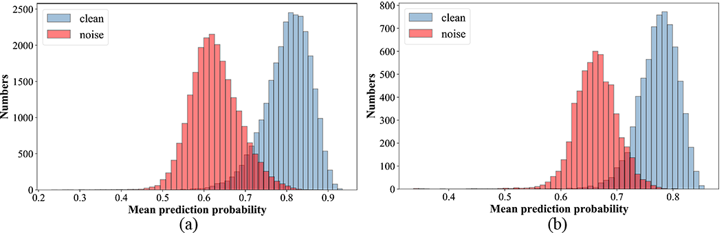
Figure 4: (a) Mean prediction probability histogram of the clean and noisy samples in CIFAR-10 ($D$) with 50% symmetric noise. (b) Mean prediction probability histogram of the clean and noisy samples in corresponding $D_{a}$.

Why $D_{a}$ Works?

To study why $M_{m}$ trained on the artificial created $D_{a}$ can recognize hard and noisy samples in original dataset $D$, we plotted both the mean prediction probability histogram of the clean and noisy samples in CIFAR-10 (50% symmetric noise ratio) $D$ and the corresponding $D_{a}$. The results are shown in Figure 4. According to Figure 4(b), there are also some clean samples which can not be distinguished from the noisy ones by mean prediction probability. Although the samples in $D_{e}$ are all easy ones to dataset $D$, part of the samples became hard ones to dataset $D_{a}$. In Figure 4, it should be noted that the mean prediction probabilities of samples trained on $D_{a}$ have similar distribution with the original dataset $D$, and this is why our Prior Generation Module works by using the artificial created $D_{a}$.

Work with Other SSL Methods

To utilize the samples which were divided into noisy set, we used MixMatch (Berthelot et al. 2019) in Section Denoising with the Divided Sets while other SSL methods are also applicable. We found that FixMatch (Sohn et al. 2020) as an alternative works even better, and achieves 75.3% accuracy in Clothing1M dataset. Our method is flexible to other SSL methods. However, these augmentation strategies are not the focus of this paper.

Limitations

The quantifiable behavioral differences between hard and noisy samples are not clear. There could exist other better metrics that can be used to directly distinguish them. Our subsequent work will continue to investigate specific quantifiable metrics to simplify the process of the Prior Generation Module, and how to strengthen hard samples more reasonably is a direction worth studying in the future.

Conclusions

The existing methods for learning with noisy labels fail to distinguish the hard samples from the noisy ones and thus ruin the model performance. In this paper, we propose PGDF to learn a deep model to suppress noise. We found that the training history can be used to distinguish the hard samples and noisy samples. By integrating our Prior Generation, more hard clean samples can be saved. Besides, our pseudo-labels refining and hard enhancing phase further boost the performance. Through extensive experiments show that PGDF outperforms state-of-the-art performance.

Appendix A Appendix

Additional Experiment Results

Note that there is another criterion for symmetric label noise injection where the true labels cannot be maintained. Work (Wu et al. 2020) reported the results with the average test accuracy and standard deviation in this criterion. We use the same backbone (ResNet-18 (He et al. 2016a)) and follow the same metrics as work (Wu et al. 2020). The results are reported in Table 8. Our method outperforms all other baselines by a large margin.

Method/Noise ratio	20%	40%	60%	80%
Standard	85.7$\pm$0.5	81.8$\pm$0.6	73.7$\pm$1.1	42.0$\pm$2.8
Forgetting(2017)	86.0$\pm$0.8	82.1$\pm$0.7	75.5$\pm$0.7	41.3$\pm$3.3
Bootstrap(2014)	86.4$\pm$0.6	82.5$\pm$0.1	75.2$\pm$0.8	42.1$\pm$3.3
Forward(2017)	85.7$\pm$0.4	81.0$\pm$0.4	73.3$\pm$1.1	31.6$\pm$4.0
Decoupling(2017)	87.4$\pm$0.3	83.3$\pm$0.4	73.8$\pm$1.0	36.0$\pm$3.2
MentorNet(2018)	88.1$\pm$0.3	81.4$\pm$0.5	70.4$\pm$1.1	31.3$\pm$2.9
Co-teaching(2018)	89.2$\pm$0.3	86.4$\pm$0.4	79.0$\pm$0.2	22.9$\pm$3.5
Co-teaching+(2019)	89.8$\pm$0.2	86.1$\pm$0.2	74.0$\pm$0.2	17.9$\pm$1.1
IterNLD(2018)	87.9$\pm$0.4	83.7$\pm$0.4	74.1$\pm$0.5	38.0$\pm$1.9
RoG(2019)	89.2$\pm$0.3	83.5$\pm$0.4	77.9$\pm$0.6	29.1$\pm$1.8
PENCIL(2019)	88.2$\pm$0.2	86.6$\pm$0.3	74.3$\pm$0.6	45.3$\pm$1.4
GCE(2018)	88.7$\pm$0.3	84.7$\pm$0.4	76.1$\pm$0.3	41.7$\pm$1.0
SL(2019)	89.2$\pm$0.5	85.3$\pm$0.7	78.0$\pm$0.3	44.4$\pm$1.1
TopoCC(2020)	89.6$\pm$0.3	86.0$\pm$0.5	78.7$\pm$0.5	43.0$\pm$2.0
TopoFilter(2020)	90.2$\pm$0.2	87.2$\pm$0.4	80.5+0.4	45.7$\pm$1.0
PGDF(ours)	96.50$\pm$0.13	96.18$\pm$0.17	95.19$\pm$0.38	82.15$\pm$1.94

Table 8: Average test accuracy (%) and stardard deviation on CIFAR-10 with symmetric noise (ranging from 20% to 80%). Results for previous techniques were directly copied from (Wu et al. 2020).

Hyper-parameters Analysis

In order to analyze the sensitivity of the hyper-parameters proposed in this paper, we conduct experiments on CIFAR-10 dataset with 50% symmetric noise ratio. Specifically, we first fixed the hyper-parameters settings as $m=0.5$, $r=2$, $k=300$, $\tau_{e}=0.25$, and $\tau_{n1}=0.25$, then change the value of each hyper-parameter respectively to obtain the sensitivity. The results are shown in Table 9. According to Table 9, for $m$ and $r$, the performances of the model increase first, then achieve the peak, and finally decrease with the increase of each parameter. For $k$, the performance first increases, and then becomes relatively stable when $k$ exceeds a certain threshold. It should be noted that $m=0$ is equivalent to the ablation study “PGDF w/o prior knowledge”, and $m=1$ is equivalent to the ablation study “PGDF w/o sample dividing optimization”.

Table 9: Results in terms of average test accuracy (%, 3 runs) with standard deviation on different “$m$”, “$r$” and “$k$” on CIFAR-10 with 50% symmetric noise ratio.

$m$	0	0.25	0.5	0.75	1
best	95.73$\pm$0.09	95.86$\pm$0.14	96.26$\pm$0.09	95.99$\pm$0.11	95.55$\pm$0.11
last	95.50$\pm$0.12	95.73$\pm$0.16	96.15$\pm$0.13	95.92$\pm$0.12	95.13$\pm$0.19
$r$	1	2	3	4
best	96.17$\pm$0.07	96.26$\pm$0.09	96.03$\pm$0.17	95.61$\pm$0.23
last	96.00$\pm$0.13	96.15$\pm$0.13	95.80$\pm$0.23	95.40$\pm$0.31
$k$	100	200	300	400
best	95.74$\pm$0.13	96.08$\pm$0.08	96.26$\pm$0.09	96.23$\pm$0.10
last	95.59$\pm$0.15	95.89$\pm$0.13	96.15$\pm$0.13	96.07$\pm$0.18

Hard and Noisy Sample Behavior Analysis

To analyze the training process behavior of the hard sample and the noise sample, inspired by (Toneva et al. 2018), we randomly selected 1000 hard samples, 1000 noisy samples on CIFAR-10 with 20% symmetric noise, and calculated the number of “Learning” event and “Forgetting” event of them through the training epochs. The “Learning” event in the $t$ epoch is defined as the prediction probability of the labeled class is less than $0.5$ in $t-1$ epoch, while greater than $0.5$ in $t$ epoch. The “Forgetting” event in the $t$ epoch is defined as the prediction probability of the labeled class is greater than $0.5$ in $t-1$ epoch, while less than $0.5$ in $t$ epoch. The statistical result is shown in Figure 5.

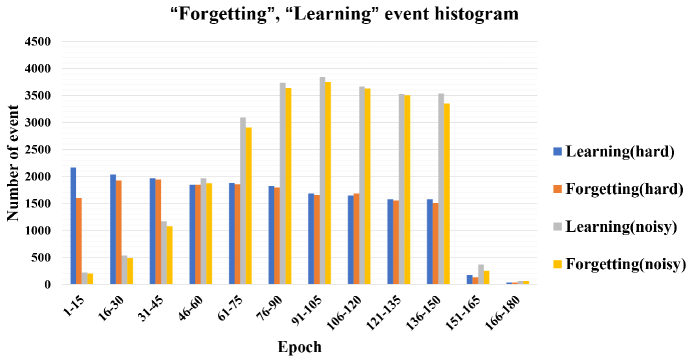
Figure 5: The forgetting and learning event histogram on CIFAR-10 with 20% symmetric noise.

This result shows that the hard sample and the noisy sample have great behavioral differences with the increase of the epoch in training. Before the model converges, the number of learning events and forgetting events of noisy samples is relatively small in the early training stage, and gradually increases as the number of training epochs increases. The learning forgetting events of hard samples are relatively consistent throughout the training process.

Training Time Report

We recorded the training time of different steps of PGDF on CIFAR-10 with 50% symmetric noise by using a single Nvidia V100 GPU. The results are shown in Table 10.

Table 10: Different steps of training time (hours) on CIFAR-10 with 50% symmetric noise.

Prior Generation Module	Subsequent training process	All
2.1 h	8.2 h	10.3 h

References

- Arazo et al. (2019) Arazo, E.; Ortego, D.; Albert, P.; O’Connor, N.; and McGuinness, K. 2019. Unsupervised label noise modeling and loss correction. In International Conference on Machine Learning, 312–321. PMLR.
- Berthelot et al. (2019) Berthelot, D.; Carlini, N.; Goodfellow, I.; Papernot, N.; Oliver, A.; and Raffel, C. 2019. Mixmatch: A holistic approach to semi-supervised learning. In Advances in Neural Information Processing Systems 32: Annual Conference on Neural Information Processing Systems.
- Chen et al. (2019) Chen, P.; Liao, B.; Chen, G.; and Zhang, S. 2019. Understanding and Utilizing Deep Neural Networks Trained with Noisy Labels. arXiv preprint arXiv:1905.05040.
- Chen et al. (2021) Chen, P.; Ye, J.; Chen, G.; Zhao, J.; and Heng, P.-A. 2021. Beyond Class-Conditional Assumption: A Primary Attempt to Combat Instance-Dependent Label Noise. In Proceedings of the AAAI Conference on Artificial Intelligence.
- Cordeiro et al. (2021) Cordeiro, F. R.; Sachdeva, R.; Belagiannis, V.; Reid, I.; and Carneiro, G. 2021. LongReMix: Robust Learning with High Confidence Samples in a Noisy Label Environment. arXiv preprint arXiv:2103.04173.
- Ghosh, Kumar, and Sastry (2017) Ghosh, A.; Kumar, H.; and Sastry, P. 2017. Robust loss functions under label noise for deep neural networks. In Thirty-First AAAI Conference on Artificial Intelligence.
- Goldberger and Ben-Reuven (2017) Goldberger, J.; and Ben-Reuven, E. 2017. Training deep neural-networks using a noise adaptation layer. In 5th International Conference on Learning Representations.
- Han et al. (2018) Han, B.; Yao, Q.; Yu, X.; Niu, G.; Xu, M.; Hu, W.; Tsang, I.; and Sugiyama, M. 2018. Co-teaching: Robust training of deep neural networks with extremely noisy labels. In Advances in neural information processing systems, 8527–8537.
- Han, Luo, and Wang (2019) Han, J.; Luo, P.; and Wang, X. 2019. Deep self-learning from noisy labels. In Proceedings of the IEEE/CVF International Conference on Computer Vision, 5138–5147.
- He et al. (2016a) He, K.; Zhang, X.; Ren, S.; and Sun, J. 2016a. Deep residual learning for image recognition. In Proceedings of the IEEE conference on computer vision and pattern recognition, 770–778.
- He et al. (2016b) He, K.; Zhang, X.; Ren, S.; and Sun, J. 2016b. Identity Mappings in Deep Residual Networks. In European Conference on Computer Vision.
- Huang et al. (2019) Huang, J.; Qu, L.; Jia, R.; and Zhao, B. 2019. O2u-net: A simple noisy label detection approach for deep neural networks. In Proceedings of the IEEE/CVF International Conference on Computer Vision, 3326–3334.
- Jiang et al. (2018) Jiang, L.; Zhou, Z.; Leung, T.; Li, L.-J.; and Fei-Fei, L. 2018. Mentornet: Learning data-driven curriculum for very deep neural networks on corrupted labels. In International Conference on Machine Learning, 2304–2313. PMLR.
- Krizhevsky and Hinton (2009) Krizhevsky, A.; and Hinton, G. 2009. Learning multiple layers of features from tiny images. Handbook of Systemic Autoimmune Diseases, 1(4).
- Krizhevsky, Sutskever, and Hinton (2012) Krizhevsky, A.; Sutskever, I.; and Hinton, G. E. 2012. Imagenet classification with deep convolutional neural networks. In Advances in neural information processing systems, 1097–1105.
- Li, Socher, and Hoi (2020) Li, J.; Socher, R.; and Hoi, S. 2020. DivideMix: Learning with Noisy Labels as Semi-supervised Learning.
- Li et al. (2019) Li, J.; Wong, Y.; Zhao, Q.; and Kankanhalli, M. S. 2019. Learning to Learn From Noisy Labeled Data. In 2019 IEEE/CVF Conference on Computer Vision and Pattern Recognition (CVPR).
- Liu et al. (2020) Liu, S.; Niles-Weed, J.; Razavian, N.; and Fernandez-Granda, C. 2020. Early-Learning Regularization Prevents Memorization of Noisy Labels.
- Lyu and Tsang (2019) Lyu, Y.; and Tsang, I. W. 2019. Curriculum Loss: Robust Learning and Generalization against Label Corruption.
- Montserrat et al. (2017) Montserrat, D. M.; Lin, Q.; Allebach, J.; and Delp, E. J. 2017. Training object detection and recognition CNN models using data augmentation. Electronic Imaging, 2017(10): 27–36.
- Nishi et al. (2021) Nishi, K.; Ding, Y.; Rich, A.; and Hllerer, T. 2021. Augmentation Strategies for Learning with Noisy Labels. In Proceedings of the IEEE/CVF Conference on Computer Vision and Pattern Recognition (CVPR).
- Patrini et al. (2017) Patrini, G.; Rozza, A.; Krishna Menon, A.; Nock, R.; and Qu, L. 2017. Making deep neural networks robust to label noise: A loss correction approach. In Proceedings of the IEEE Conference on Computer Vision and Pattern Recognition, 1944–1952.
- Ren et al. (2018) Ren, M.; Zeng, W.; Yang, B.; and Urtasun, R. 2018. Learning to Reweight Examples for Robust Deep Learning.
- Russakovsky et al. (2015) Russakovsky, O.; Deng, J.; Su, H.; Krause, J.; Satheesh, S.; Ma, S.; Huang, Z.; Karpathy, A.; Khosla, A.; Bernstein, M.; et al. 2015. Imagenet large scale visual recognition challenge. International journal of computer vision, 115(3): 211–252.
- Sarfraz, Arani, and Zonooz (2020) Sarfraz, F.; Arani, E.; and Zonooz, B. 2020. Noisy Concurrent Training for Efficient Learning under Label Noise.
- Sohn et al. (2020) Sohn, K.; Berthelot, D.; Li, C.-L.; Zhang, Z.; Carlini, N.; Cubuk, E. D.; Kurakin, A.; Zhang, H.; and Raffel, C. 2020. FixMatch: Simplifying Semi-Supervised Learning with Consistency and Confidence. arXiv preprint arXiv:2001.07685.
- Song et al. (2019) Song, H.; Kim, M.; Park, D.; and Lee, J. G. 2019. Prestopping: How Does Early Stopping Help Generalization against Label Noise?
- Sun et al. (2019) Sun, Y.; Tian, Y.; Xu, Y.; and Li, J. 2019. Limited Gradient Descent: Learning With Noisy Labels. IEEE Access, 7: 168296–168306.
- Szegedy et al. (2017) Szegedy, C.; Ioffe, S.; Vanhoucke, V.; and Alemi, A. A. 2017. Inception-v4, inception-ResNet and the impact of residual connections on learning.
- Tanno et al. (2020) Tanno, R.; Saeedi, A.; Sankaranarayanan, S.; AleXaNder, D. C.; and Silberman, N. 2020. Learning From Noisy Labels by Regularized Estimation of Annotator Confusion. In 2019 IEEE/CVF Conference on Computer Vision and Pattern Recognition (CVPR).
- Thulasidasan et al. (2019) Thulasidasan, S.; Bhattacharya, T.; Bilmes, J.; Chennupati, G.; and Mohd-Yusof, J. 2019. Combating label noise in deep learning using abstention. arXiv preprint arXiv:1905.10964.
- Toneva et al. (2018) Toneva, M.; Sordoni, A.; Combes, R. T. d.; Trischler, A.; Bengio, Y.; and Gordon, G. J. 2018. An empirical study of example forgetting during deep neural network learning. arXiv preprint arXiv:1812.05159.
- Tong et al. (2015) Tong, X.; Tian, X.; Yi, Y.; Chang, H.; and Wang, X. 2015. Learning from massive noisy labeled data for image classification. In 2015 IEEE Conference on Computer Vision and Pattern Recognition (CVPR).
- Wang et al. (2019) Wang, Y.; Ma, X.; Chen, Z.; Luo, Y.; Yi, J.; and Bailey, J. 2019. Symmetric cross entropy for robust learning with noisy labels. In Proceedings of the IEEE/CVF International Conference on Computer Vision, 322–330.
- Wei et al. (2019) Wei, Y.; Gong, C.; Chen, S.; Liu, T.; Yang, J.; and Tao, D. 2019. Harnessing Side Information for Classification Under Label Noise. IEEE Transactions on Neural Networks and Learning Systems.
- Wen et al. (2017) Wen, L.; Wang, L.; Wei, L.; Agustsson, E.; and Gool, L. V. 2017. WebVision Database: Visual Learning and Understanding from Web Data.
- Wu et al. (2020) Wu, P.; Zheng, S.; Goswami, M.; Metaxas, D.; and Chen, C. 2020. A Topological Filter for Learning with Label Noise. In Advances in Neural Information Processing Systems 33 pre-proceedings (NeurIPS 2020).
- Wu et al. (2021) Wu, Z.-F.; Wei, T.; Jiang, J.; Mao, C.; Tang, M.; and Li, Y.-F. 2021. NGC: A Unified Framework for Learning with Open-World Noisy Data. arXiv preprint arXiv:2108.11035.
- Xiao et al. (2015) Xiao, T.; Xia, T.; Yang, Y.; Huang, C.; and Wang, X. 2015. Learning from massive noisy labeled data for image classification. In Proceedings of the IEEE conference on computer vision and pattern recognition, 2691–2699.
- Xu et al. (2019) Xu, Y.; Cao, P.; Kong, Y.; and Wang, Y. 2019. L_dmi: An information-theoretic noise-robust loss function. arXiv preprint arXiv:1909.03388.
- Yi and Wu (2019) Yi, K.; and Wu, J. 2019. Probabilistic End-to-end Noise Correction for Learning with Noisy Labels. arXiv preprint arXiv:1903.07788.
- Young et al. (2018) Young, T.; Hazarika, D.; Poria, S.; and Cambria, E. 2018. Recent trends in deep learning based natural language processing. ieee Computational intelligenCe magazine, 13(3): 55–75.
- Yu et al. (2019) Yu, X.; Han, B.; Yao, J.; Niu, G.; Tsang, I. W.; and Sugiyama, M. 2019. How does Disagreement Help Generalization against Label Corruption?
- Zhang et al. (2016) Zhang, C.; BeNgio, S.; Hardt, M.; Recht, B.; and Vinyals, O. 2016. Understanding deep learning requires rethinking generalization.
- Zhang et al. (2018) Zhang, H.; Cisse, M.; Dauphin, Y. N.; and Lopez-Paz, D. 2018. mixup: Beyond Empirical Risk Minimization.
- Zhang and Sabuncu (2018) Zhang, Z.; and Sabuncu, M. 2018. Generalized cross entropy loss for training deep neural networks with noisy labels. In Advances in neural information processing systems, 8778–8788.
- Zheltonozhskii et al. (2022) Zheltonozhskii, E.; Baskin, C.; Mendelson, A.; Bronstein, A. M.; and Litany, O. 2022. Contrast to divide: Self-supervised pre-training for learning with noisy labels. In Proceedings of the IEEE/CVF Winter Conference on Applications of Computer Vision, 1657–1667.
- Zhou et al. (2021a) Zhou, X.; Liu, X.; Jiang, J.; Gao, X.; and Ji, X. 2021a. Asymmetric Loss Functions for Learning with Noisy Labels. arXiv preprint arXiv:2106.03110.
- Zhou et al. (2021b) Zhou, X.; Liu, X.; Wang, C.; Zhai, D.; Jiang, J.; and Ji, X. 2021b. Learning with Noisy Labels via Sparse Regularization. In Proceedings of the IEEE/CVF International Conference on Computer Vision, 72–81.
- Zhu, Liu, and Liu (2021) Zhu, Z.; Liu, T.; and Liu, Y. 2021. A second-order approach to learning with instance-dependent label noise. In Proceedings of the IEEE/CVF Conference on Computer Vision and Pattern Recognition, 10113–10123.