Chapter 1 Stability of plasmas through magnetic helicity

   Fabio Del Sordo

[1]Simon Candelaresi

Abstract

Abstract Magnetic helicity, and more broadly magnetic field line topology, imposes constraints on the plasma dynamics. Helically interlocked magnetic rings are harder to bring into a topologically non-trivial state than two rings that are not linked. This particular restriction has the consequence that helical plasmas exhibit increased stability in laboratory devices, in the Sun and in the intergalactic medium. Here we discuss how a magnetic field is stabilizing the plasma and preventing it from disruption by the presence of magnetic helicity. We present observational results, numerical experiments and analytical results that illustrate how helical magnetic fields strongly contribute to the long-term stability of some plasmas. We discuss several cases, such as that of solar corona, tokamaks, the galactic and extragalactic medium, with a special emphasis on extragalactic bubbles.

1.1 Introduction

In the context of magnetohydrodynamics (MHD), the physics of magnetized fluids, helical magnetic fields are known to play a special role. They are important both in the context of magnetic field amplification (e.g. BS05; 2016MNRAS.461..240B), and for the characterization of the saturation stage of magnetic field evolution in MHD instabilities (e.g. 2011PhRvE..84b5403C; BBDSM12). In this work we discuss the importance of helicity conservation law (e.g. 1987ApJ...319..207B) for the evolution and the stability of plasmas. Large-scale magnetic helicity is known to stabilize plasmas in different contexts. One remarkable example is that of coronal mass ejections (CMEs) on our Sun: they are aided by the presence of an internal twist within the raising and the erupting plasma patches (Canfield1996b). With a topologically trivial and non-helical internal field CMEs would disintegrate before reaching the solar photosphere.

There are two formalisms that tell us how magnetic helicity acts as a stabilizer of the system. One is the near helicity conservation in most astrophysical systems with their high magnetic Reynolds numbers. The other is the realizability condition (ArnoldHopf1986) which poses a lower bound of the magnetic energy in presence of helicity.

However, helicity acts not only as stabilizer. As magnetic fields are wound up and braided continuously, they may be subject of an MHD instability, the kink instability (e.g. 2013SoPh..287..185B). For the Sun, on the other hand, the induced braiding in solar coronal loops does not seem to be sufficient for this instability (Aschwanden-2019-874-131-AAS).

Here we will give an account how magnetic helicity plays and important role in the plasma’s stability, particularly in the context of astrophysical magnetic fields. Those range from small scales found in fusion devices up to kiloparsec sized plasmas in the intergalactic medium.

In this paper we will start by illustrating in Sec. 1.2 how the magnetic helicity conservation works. Then we will deal in Sec. 1.3 with the final equilibrium state that should be reached by plasmas, and with the constraints that play a role in reaching this equilibrium (Sec. 1.4). In Sec. 1.5 we will see some examples of plasmas which reach stability as consequence of the existence of large-scale magnetic helicity, whilst we will concentrate on examples of plasmas on galactic and intergalactic scales in Sec. 1.6. In Sec. 1.7 we will then move to a specific example, that of intergalactic cavities, for which a mechanism of stabilization through large-scale magnetic helicity has been recently proposed. Finally, we will draw some conclusions in Sec. 1.8.

1.2 Helicity Conservation

The conservation of magnetic helicity in high magnetic Reynolds number regimes can be easily derived from the magnetohyrodynamics equations for a resistive, viscous compressible gas (e.g. Biskamp-2003-Magnetohydrodynamic_Turbulence):

$$\frac{\partial\mbox{\boldmath$A$}{}}{\partial t}=\mbox{\boldmath$u$}{}\times\bm{B}+\eta\nabla^{2}\mbox{\boldmath$A$}{},$$ (1.1)

$$\frac{{\rm D}{}\mbox{\boldmath$u$}{}}{{\rm D}{}t}=-c_{\rm s}^{2}\mbox{\boldmath$\nabla$}{}\ln{\rho}+\mbox{\boldmath$J$}{}\times\bm{B}/\rho+\mbox{\boldmath$F$}{}_{\rm visc},$$ (1.2)

$$\frac{{\rm D}{}\ln{\rho}}{{\rm D}{}t}=-\mbox{\boldmath$\nabla$}{}\cdot\mbox{\boldmath$u$}{},$$ (1.3)

with the magnetic vector potential $A$, velocity $u$, magnetic field $\bm{B}=\mbox{\boldmath$\nabla$}{}\times\mbox{\boldmath$A$}{}$, magnetic resistivity $\eta$, isothermal speed of sound $c_{\rm s}$, density $\rho$, current density $\mbox{\boldmath$J$}{}=\mbox{\boldmath$\nabla$}{}\times\bm{B}$, viscous forces $\mbox{\boldmath$F$}{}_{\rm visc}$ and Lagrangian time derivative ${\rm D}{}/{\rm D}{}t=\partial/\partial t+\mbox{\boldmath$u$}{}\cdot\mbox{\boldmath$\nabla$}{}$. Here the viscous forces are given as $\mbox{\boldmath$F$}{}_{\rm visc}=\rho^{-1}\mbox{\boldmath$\nabla$}{}\cdot 2\nu\rho\mbox{\boldmath$S$}{}$, with the kinematic viscosity $\nu$, and traceless rate of strain tensor $\mbox{\boldmath$S$}{}_{ij}=\frac{1}{2}(u_{i,j}+u_{j,i})-\frac{1}{3}\delta_{ij}\mbox{\boldmath$\nabla$}{}\cdot\mbox{\boldmath$u$}{}$. Being an isothermal gas we have $p=c_{\rm s}^{2}\rho$ for the pressure.

Here we use the induction equation (1.1) expressed using the magnetic vector potential $A$ instead of the magnetic field $\bm{B}$. This has a few advantages. First, we can directly compute the magnetic helicity density

$$h_{\rm m}=\mbox{\boldmath$A$}{}\cdot\bm{B}$$ (1.4)

in all space for all times without the need of finding the inverse curl. Second, the solenoidal condition of $\mbox{\boldmath$\nabla$}{}\cdot\bm{B}=0$ is trivially fulfilled. This is particularly useful in numerical calculations as it is ensure not to incur in non-zero-divergence $\bm{B}$, which could potentially lead to spurious results (see e.g. BrandScann2020ApJ...889...55B). Of course, we are still left with the gauge choice here, since the vector potential $\mbox{\boldmath$A$}{}^{\prime}=\mbox{\boldmath$A$}{}+\mbox{\boldmath$\nabla$}{}\phi$, with the differentiable scalar field $\phi$, leads to the same vector field $\bm{B}=\mbox{\boldmath$\nabla$}{}\times\mbox{\boldmath$A$}{}^{\prime}$. The implicit gauge in our induction equation is the the Coulomb gauge with $\mbox{\boldmath$\nabla$}{}\cdot\mbox{\boldmath$A$}{}=0$.

From the MHD equations we can now derive the rate of change in time of the magnetic helicity as

$$\partial_{t}H_{\rm m} = \int_{V}\partial_{t}\mbox{\boldmath$A$}{}\cdot\bm{B}+\mbox{\boldmath$A$}{}\cdot\partial_{t}\bm{B}$$ (1.6)

$$= -2\eta\int_{V}\mbox{\boldmath$J$}{}\cdot\bm{B}\ {\rm d}{}V+$$

$$\int_{\partial V}\mbox{\boldmath$A$}{}\times(\bm{B}\times\mbox{\boldmath$u$}{}+\mbox{\boldmath$J$}{})\cdot{\rm d}{}\mbox{\boldmath$S$}{}.$$

The first term is the resistive helicity dissipation/generation term. For turbulent dissipative systems, the electric current density and magnetic field are on average aligned. This makes this term in practice a dissipation term. The last two terms are surface terms. They have the potential of helicity injection or helicity loss in a finite domain. For instance, this is the case for domains located in the solar atmosphere or bordering the solar photosphere. In these cases, the fields are finite and there is a possible helicity flux through the surface, even for small diffusivities, as the diffusivity does not enter the surface terms. The same concept applies on large scales, such as galaxies, who may experience helicity loss through the halo and then to extragalactig medium. This helicity flux may be relevant for galactic dynamo (2020A&A...641A.165N) and may play a key role for galactic magnetic fields to reach the observed values (2013MNRAS.429.1686D; 2021arXiv210812037R).

For systems with periodic boundaries, closed boundaries, or where the boundaries are so far that our quantities can be considered zero, the surface terms vanish. In that case we can focus on the resistive dissipation term. This dissipation is small for most astrophysical settings, as $\eta$ is so small that structures of the size in question diffuse on much longer time scales than the typical dynamical time scales. So, we can assume that magnetic helicity is conserved in such systems.

In the limit of vanishing magnetic diffusion ($\eta=0$) the induction equation (1.1) simplifies to

$$\frac{\partial\mbox{\boldmath$A$}{}}{\partial t}=\mbox{\boldmath$u$}{}\times\bm{B},$$ (1.7)

or, expressed in terms of the magnetic field $\bm{B}$, we can write

$$\frac{\partial\bm{B}}{\partial t}=\mbox{\boldmath$\nabla$}{}\times(\mbox{\boldmath$u$}{}\times\bm{B}).$$ (1.8)

This last equation describes a magnetic field that is simply Lie-transported under the velocity field $u$ (mimetic14). We than say that the field is “frozen in” into the fluid (Alfven-1942-150-405-Nature; BatchelorFrozeIn1950RSPSA; PriestReconnection2000). In simple term, a gas/fluid compression perpendicular to $\bm{B}$ increases the local magnetic field strength by the compression factor. We can also show that every open advected surface $S$ preserves its magnetic flux

$$\Phi=\int_{S}\bm{B}\cdot{\rm d}{}S.$$ (1.9)

More formally, this can be expressed in terms of differential two-forms $\beta=B_{x}{\rm d}{}y\wedge{\rm d}{}z+B_{y}{\rm d}{}z\wedge{\rm d}{}x+B_{z}{\rm d}{}x\wedge{\rm d}{}y$

$$\frac{{\rm d}{}}{{\rm d}{}t}\beta=\mathcal{L}_{\mbox{\boldmath$u$}{}}(\beta),$$ (1.10)

where $\mathcal{L}_{\mbox{\boldmath$u$}{}}(\beta)$ is the Lie-transport of $\beta$ under the velocity $u$.

Being the magnetic field frozen in, magnetic field lines obtain a physical meaning, as they cannot be broken up and reconnected, which is a manifestation of the restrictions in the field’s dynamics.

Together with the magnetic field, also the magnetic helicity density is being Lie-transported in the ideal limit. Being a density, this means that every advected volume $V$ preserves its helicity. Consequently, also the entire domain (being also a volume) conserves its magnetic helicity:

$$\frac{{\rm d}{}}{{\rm d}{}t}H_{\rm m}=0.$$ (1.11)

So, we have exact magnetic helicity conservation for $\eta=0$.

The discussion is similar for the case of the limit, i.e. $\lim_{\eta\rightarrow 0}$. We can perform the same calculations and arrive at the same result

$$\lim_{\eta\rightarrow 0}\frac{{\rm d}{}}{{\rm d}{}t}H_{\rm m}=0.$$ (1.12)

1.3 Relaxation Equilibrium State

What consequences does the helicity conservation have for the dynamics of the system, particularly for relaxing/decaying magnetic fields? During any stage of its evolution – this of course includes its end state – it must go through states of the same magnetic helicity. This already excludes a large class of fields, like those with a connectivity with a different magnetic helicity.

So, similar to the energy conservation in a non-dissipative system like a pendulum, we can already make predictions about what behavior is excluded and, to some extend, make qualitative predictions about the geometry of the magnetic field lines during the evolution.

For a field in a non-equilibrium state, we know that it will try to reach a minimum energy state. This is true for any relaxing magnetic fields in a closed or infinitely large MHD system. Without any constraints, this lowest energy would simply be zero. Woltjer-1958-489-91-PNAS showed that under magnetic helicity conservation, the lowest magnetic energy state is the force-free state with $\mbox{\boldmath$\nabla$}{}\times\bm{B}=\alpha\bm{B}$, where $\alpha$ is the force-free parameter. If this state can be reached may depend on the geometry of the field and its topology not captured by helicity. For instance, if the minimum energy state can only be reached by magnetic field line reconnection, it won’t be accessible under ideal evoution.

Since in the ideal ($\eta=0$) case the field evolves under a Lie-transport, every advected sub-volume of the domain conserves its helicity. In particular, every finite neighborhood of the magnetic field lines, conserves it helicity content. For closed field lines of finite length this can be easily imagined. We then simply have infinitesimally thin magnetic closed flux tubes (potentially knotted or braided) that conserve helicity. This is true for all neighboring flux tubes that may contain a different amount of helicity. For ergodic field lines, that fill a finite space in three dimensions, the interpretation becomes more interesting. In that case we have a constant helicity not just on a sub-volume with measure $0$, but with potentially a finite measure and finite volume.

With the helicity conservation for every magnetic field line Taylor-1974-PrlE considered the conservation of helicity, not just globally, but for every subvolume bounded by the field lines where he defined sub-helicities for each sub-volume. The minimum energy state (relaxed state) is a non-linear force-free field where the force-free parameter $\alpha$ depends on the field line:

$$\mbox{\boldmath$\nabla$}{}\times\bm{B}=\alpha(a,b)\bm{B}.$$ (1.13)

This is known as Taylor relaxation. For ergodic field lines we then have finite volumes with the same parameter $\alpha$, as we are dealing with the same field line.

1.4 Field Relaxation Constraints

From the above discussion by Woltjer and Taylor we cannot deduce if the given magnetic field will ever reach such an equilibrium. It can well be that topological constraints inhibit the plasma to even get close to a linear or non-linear force-free state.

One such constraint is given by the realizability condition (ArnoldHopf1986). It defines a lower limit for the magnetic energy in presence of magnetic helicity as

$$E(k)\geq k|H(k)|,$$ (1.14)

where $k$ is the inverse wavelength. This can be integrated over the parameter $k$, which results into a global constraint. In an experiment or numerical simulation this effect can be easily observed by comparing the magnetic helicity with the magnetic energy. After some initial free relaxation with a drop in energy, the energy reaches a near constant value in low resistivity environments. Independent of the magnetic resistivity, the ratio of the two quantities will reach a near constant.

For a purely hydrodynamical case that follows the compressible viscous Navier-Stokes equations, an analogous exact relation exists. But instead of relating the kinetic energy to the kinetic helicity the relation is between the kinetic helicity and the enstrophy, which is the volume integral of the vorticity squared. It can be easily derived that the enstrophy is bound from below by the kinetic helicity (vortex_braids). Although with no existing exact relation, the same authors found expirementally a similar realizability condition that limits the kinetic energy from below by the presence of unsigned kinetic helicity.

A naïve interpretation of the realizability condition can be drawn from a simple thought experiment. Take two closed magnetic flux tubes, with no internal twist, that are linked with each other once. This configuration is helical. A minimum energy state cannot be reached, without reconnection. However, we can conceive an experiment with three linked fluxtubes and by defining the correct signs of the magnetic field in each tube, we can make this configuration non-helical. This puts us into a slightly troubled situation, as the naïve interpretation of the realizability breaks down. From numerical experiments by DS2010PhRvE, we know that the actual linking plays only a minor role, while the helicity content poses the real restrictions, as expressed in the realizability condition.

1.5 Plasma Stability

1.5.1 Solar Eruptions

Analyzing soft X-ray images of solar active regions, Canfield1999 showed that sigmoidal structure are more likely to result into solar eruptions compared to non-sigmoidal structures. Sigmoids are a result of magnetic flux tube twisting where an increase in twist leads to kinking. These flux tubes are generated below the photosphere where they can obtain their internal twist from the solar rotation. As they rise through the convection zone some of them disrupt and do not pinch through the photosphere as an intact fluxtube. Those that are helical, however, survive long enough and may result into a coronal mass ejections at later times (Gibson2002).

While the twist leads to stability below the photosphere, it can also lead to a kink instability, if it is sufficiently high (e.g. Finkelstein-Weil-1978-17-201-IntJTheoPhys; Craig-Sneyd-1990-357-653-ApJ; RustKumar1996ApJ; Ebrahimi-Karami-2016-162-1002-MNRAS; Vemareddy-Gopalswamy-2017-850-38-ApJ). Such high fluxtube twists can be generated through photospheric motions (Canfield1999).

At the same time, an induced twist into a more complex photospheric magnetic loop structure has the potential to move the fluxtubes around, such that reconnection may occur. Even on a scale relatively small, such as that of sunspots, helicity can be induced into fluxtubes via sunspot rotation (e.g. Wang-Liu-2016-SolPhys). These reconnection events lead to a high electric current density and with that a high particle acceleration. Such events may not be coronal mass ejection, but rather bright flares that can be observed in white light or in extreme ultra violet.

1.5.2 Tokamak Fields

A tokamak is a device aimed at producing controlled fusion reactions in hot plasma. In order to confine the plasma in the shape of a torus, strong magnetic fields are used. A helical magnetic field in tokamak plasma can easily maintain its energy: this is evident from the realizability condition (1.14). Such a helical field can be generated by two currents. One is poloidal, i.e. a ring current around the torus’ main axis. The other component is a current along the main axis, which can artificially injected.

From Taylor-1974-PrlE and Taylor1986 we know that without any energy input, the magnetic field relaxes into a force-free state with $\nabla\times\bm{B}=\alpha\bm{B}$. This is the minimum energy state under helicity conservation. Therefore we can deduce the minimum energy input that is required to keep the plasma in a stable configuration and hence allows to maintain it in a stationary state.

1.5.3 Numerical Experimental Evidence

In order to understand the mechanism behind the stabilizing effect of the magnetic helicity in plasmas it is useful to conduct a series of experiments. Real world experiments do currently not have the power to measure the mechanisms in sufficient detail. But we need to know about the magnetic field relaxation mechanism, the nature of the reconnection events and the energy conversion sites (magnetic to kinetic/thermal).

A way out of this is by modelling the plasma using appropriate equations. For a non-relativistic plasma, as we assume the solar, glactic and tokamak plasmas to be, we can make use of the MHD equations (1.1)-(1.3).

From a purely geometrical interpretation one can argue that linking (helicity) is a stabilizer by preventing/restricting the flux tubes to reconnect arbitrarily. An early numerical experiment was devised by DS2010PhRvE. They inserted three magnetic flux rings into a box (initial condition). Two outer rings were linked to the inner ring, resulting into a linked configuration. By changing the sign of the magnetic flux of one of the outer rings they were able to change the system from one with net magnetic helicity to no magnetic helicity. A control configuration with three un-linked flux tubes was also used. With the non-helical field relaxing similarly to the trivial non-linked field it was shown that it is the helicity, rather than the actual linkage that restricts the field relaxation.

Similar experiments were carried out by C2011PhRvE where they studied the relaxation of helical and non-helical knots. One of their results was that topologically non-trivial and non-helical knots show a kind of intermediate stability between the topologically trivial fields and the helical fields. For non-helical braids Yeates_Topology_2010 observed similar enhanced stability to the trivial case. They argued that further topological invariants should be considered. The consequences would be far ranging and have implications particularly for the stability of tokamak fields. 2016A&A...587A.125P; 2016A&A...591A..16P introduced a technique for generating tubular magnetic fields with arbitrary axial geometry and internal topology with the goal of investigating the behaviour of flux ropes whose field lines have more complex entangled configurations. One of the main application of this technique is the study of flux ropes in solar corona. They concluded that magnetic field lines with sufficient complex entanglement can suppress large-scale morphological changes, and magnetic energy can be reduced through reconnection and expansion of the ropes.

1.6 Galactic and Intergalactic Medium

1.6.1 Observations

Much of the discussion in the literature on helicity in plasmas focuses on the Sun and to some lesser extent to tokamaks. In order to explain the observed large-scale fields in galaxies, magnetic helicity has been taken into account to model the magnetic field amplification through the dynamo effect. Since the parameters are unsuitable for a direct numerical simulations, many authors (KleeorinMoss2000; Sur-Shukurov-2007-377-874-MNRAS; Shukorov-Sokolov-Subramanian-Brandenburg-2008; ssHelLoss09; Chamandy-Shukurov-2014-443-1867-MNRAS; Chamandy-2016-462-4-MNRAS) have used the mean-field approach in which the given fields are separated into a fluctuating and a mean part, assuming there is scale separation.

While magnetic fields in galaxies are less studied than in stars and planets, the field in the intergalactic medium is even less well explored. From a number of X-ray observations we know that some galaxies in clusters, like Cygnus A (Carilli-Perley-1994-270-173-MNRAS) emit material through jets that forms bubble like structures above the galactic plane. The X-ray signature is a effect of the internal magnetic field that can have strengths of $$10\text{\,}\mathrm{\SIUnitSymbolMicro G}$-$40\text{\,}\mathrm{\SIUnitSymbolMicro G}$$ (Carilli-Taylor-2002-40-319-ARAA). Further observations by Taylor-Fabian-2002-334-769-MNRAS; Churazov-Bruggen-2001-554-261-ApJ; Birzan2004ApJ; McNamara-Nulsen-2007-45-117-ARAA and Montmerle-2011-51-299-EAS in different galaxy clusters, including the Virgo cluster with the galaxy M87, suggest that these lobes, or bubbles, have a higher temperature and lower density than the surrounding intergalactic medium by a factor of ca. $3$ in both. With a size of roughly $5\text{\,}\mathrm{kpc}$, they are smaller, although not significantly, than the galaxies from which they emanate. Similar observations in other galaxies, the Milky Way too displays bubbles rising above and below its midplane. They are known as Fermi bubbles, and they are known to emanate a multiwavelength radiation, from radio to $\gamma$-ray (2015ApJ...799..112C). Possible mechanisms that lead to these bubbles are galactic fountain flows (Bregman1980ApJ), the ejection of hot material through jets and the compression of the intergalactic medium (Churazov-Bruggen-2001-554-261-ApJ). Energy input from an active galactic nucleus can provide the necessary power to heat the bubbles.

The plasma in the bubbles is magnetized and relatively hot. Being hot and underdense they rise form the galactic plane much like a hot air balloon, but without membrane. This leads to a velocity shear at its boundary and should lead to the Kelvin-Helmholtz instability. Nevertheless, from measurements of their total life time (e.g. Birzan2004ApJ) we know that they can survive for $10\text{\,}\mathrm{Myr}$-$100\text{\,}\mathrm{Myr}$). This is much longer than what is estimated from the instability analysis. So, apart from their origin, one of the puzzling aspects is how they survive for such a long time.

1.6.2 Kelvin-Helmholtz Instability

In pure hydrodyanmics, a shearing flow with the velocity $\mbox{\boldmath$u$}{}=f(x)\mbox{\boldmath$e$}{}_{y}$ can be unstable, depending on the shearing flow profile $f(x)$ (typically its steepness) and the density profile of the gas (Chandrasekhar1961hhs). In its simplest form we can consider two phases. One phase consists of a fluid or gas with density $\rho_{1}$ and constant (in space) velocity $\mbox{\boldmath$u$}{}_{1}$. The other phase has density $\rho_{2}$ and parallel velocity $\mbox{\boldmath$u$}{}_{2}\neq\mbox{\boldmath$u$}{}_{1}$. Such a system, according to the Navier-Stokes equations, will not change in time. Through the Kelvin-Helmholtz instability, however, a small perturbation will be amplified exponentially, depending on the wave-length of the perturbation.

For a magnetized gas or plasma we can take the step into magnetohydrodynamics. Here, the gas and the magnetic field are coupled through the Lorentz force. Through magnetic tension building up through the fluid flow from the onsetting instability, one could imagine a stabilizing effect from the Lorentz force. Chandrasekhar1961hhs studied the effect of a homogeneous external magnetic field on the Kelvin-Helmholtz instability. There are two simple cases. One consists of a field that is perpendicular to the shearing flow ($\bm{B}_{0}\perp\mbox{\boldmath$u$}{}$). This case does not have any effect on the instability. A parallel magnetic field, however, stabilizes the system. The suppressed wavelengths depend on the strength of the field. At a field strength of

$$B^{2}\geq 2\pi(u_{1}-u_{2})^{2}(\rho_{1}\rho_{2})/(\rho_{1}+\rho_{2})$$ (1.15)

all modes are suppressed.

So, an external parallel magnetic field is a viable stabilizer for the buoyant intergalactic bubbles. Whether such a field exists or is strong enough is a matter to be determined by the observers. For comparison to our proposed stabilizing mechanism, we will discuss this case in the next section.

1.7 Helical Intergalactic Bubbles

From helical galactic dynamo models (e.g. KleeorinMoss2000; Sur-Shukurov-2007-377-874-MNRAS), we can make the assumptions that the generated magnetic field is also helical. If these bubbles originate from the galactic interior, from where they obtain their magnetic field, we can also assume that this field is helical. Being helical we can hypothesize that these bubbles have an intrinsic stability.

It is hard to make any precise predictions on the geometry and topology of this internal field. Therefore, we will discuss the effect of two different internal helical magnetic fields and their effects on the stability of the intergalactic bubbles. For more in-depth discussion and details see bubbles.

1.7.1 Numerical Experiment

To test if a helical magnetic field can stabilize the intergalactic bubbles such that they survive the observed $10\text{\,}\mathrm{-}$$100\text{\,}\mathrm{Myr}$, we performed a number of MHD simulations (bubbles). The setup consists of a underdense hot bubble surrounded by a colder stratified medium (see Figure 1.1). Buoyancy is generated by a homogeneous gravitational acceleration $g$. Since the galactic disk is larger than the bubble, a constant gravitational pull is a justified approximation and simplifies the numerical calculations.

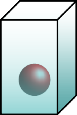
Figure 1.1: Schematic representation of the initial condition of the numerical experiment. The hot underdense bubble with homogeneous temperature and density is embedded in a stratified cold medium of higher density. The galactic disk is at the lower boundary and exerts a constant gravitational force.

In the direct numerical simulations we solve the full resistive, viscous and compressible MHD equations with the energy equation, that includes the temperature. The density and temperature contrast between bubble and medium is of a factor of $3$, which is approximately what has been observed. The numerical code used, the PencilCode (Brandenburg-Dobler-2002-147-471-CompPhysComm; Brandenburg-2020-Zenodo) (https://github.com/pencil-code) solves for the magnetic vector potential $A$, instead of the magnetic field $\bm{B}=\mbox{\boldmath$\nabla$}{}\times\mbox{\boldmath$A$}{}$. This makes sure that the solenoidal condition is fulfilled and facilitates the computation of the magnetic helicity. The equations we solve are

$$\frac{\partial\mbox{\boldmath$A$}{}}{\partial t} = \mbox{\boldmath$u$}{}\times\bm{B}+\eta\mbox{\boldmath$\nabla$}{}^{2}\mbox{\boldmath$A$}{},$$ (1.16)

$$\frac{{\rm D}{}\mbox{\boldmath$u$}{}}{{\rm D}{}t} = -c_{\rm s}^{2}\mbox{\boldmath$\nabla$}{}\left(\frac{\ln T}{\gamma}+\ln{\rho}\right)+\frac{\mbox{\boldmath$J$}{}\times\bm{B}}{\rho}$$ (1.17)

$$-\mbox{\boldmath$g$}{}+\mbox{\boldmath$F$}{}_{\rm visc},$$

$$\frac{{\rm D}{}\ln{\rho}}{{\rm D}{}t} = -\mbox{\boldmath$\nabla$}{}\cdot\mbox{\boldmath$u$}{},$$ (1.18)

$$\frac{\partial\ln T}{\partial t} = -\mbox{\boldmath$u$}{}\cdot\mbox{\boldmath$\nabla$}{}\ln T-(\gamma-1)\mbox{\boldmath$\nabla$}{}\cdot\mbox{\boldmath$u$}{}$$ (1.19)

$$+\frac{1}{\rho c_{v}T}\left(\mbox{\boldmath$\nabla$}{}\cdot(K\mbox{\boldmath$\nabla$}{}T)+\eta\mbox{\boldmath$J$}{}^{2}\right.$$

$$\left.+2\rho\nu\mbox{\boldmath${\sf S}$}{}\otimes\mbox{\boldmath${\sf S}$}{}+\zeta\rho(\mbox{\boldmath$\nabla$}{}\cdot\mbox{\boldmath$u$}{})^{2}\right),$$

with the magnetic vector potential $A$, magnetic field $\bm{B}=\mbox{\boldmath$\nabla$}{}\times\mbox{\boldmath$A$}{}$, fluid velocity $u$, constant magnetic resistivity (diffusivity) $\eta$, advective derivative ${\rm D}{}/{\rm D}{}t=\partial/\partial t+\mbox{\boldmath$u$}{}\cdot\mbox{\boldmath$\nabla$}{}$, sound speed $c_{\rm s}=\gamma p/\rho$, adiabatic index $\gamma=c_{p}/c_{v}$, heat capacities $c_{p}$ and $c_{v}$ at constant pressure and volume, temperature $T$, density $\rho$, electric current density $\mbox{\boldmath$J$}{}=\mbox{\boldmath$\nabla$}{}\times\bm{B}$, gravitational acceleration $g$, viscous force $\mbox{\boldmath$F$}{}_{\rm visc}$, heat conductivity $K$ and the bulk viscosity $\zeta$. The viscous force is given as $\mbox{\boldmath$F$}{}_{\rm visc}=\rho^{-1}\mbox{\boldmath$\nabla$}{}\cdot 2\nu\rho\mbox{\boldmath${\sf S}$}{}$, with the traceless rate of strain tensor $S_{ij}=\frac{1}{2}(u_{i,j}+u_{j,i})-\frac{1}{3}\delta_{ij}\mbox{\boldmath$\nabla$}{}\cdot\mbox{\boldmath$u$}{}$. The equation of state used here is for the ideal monatomic gas and it appears implicitly in our equations, as we eliminated pressure $p$. Here the gas is monatomic with $\gamma=5/3$.

1.7.2 Helicity as Stabilizer

Within our numerical bubble we insert a helical magnetic field. To exclude effects from the geometry of the field we use to different setups. One consists of the ABC type field of the form

$$\mbox{\boldmath$A$}{}=f(r)A_{0}\left(\begin{array}[]{c}\cos((y-y_{\rm c})k)+\sin((z-z_{\rm c})k)\\ \cos((z-z_{\rm c})k)+\sin((x-x_{\rm c})k)\\ \cos((x-x_{\rm c})k)+\sin((y-y_{\rm c})k)\end{array}\right),$$ (1.20)

where the wave number $k$ can be used to regulate the helicity relative to the magnetic energy, which is regulated by the amplitude $A_{0}$. Here the subscript c stands for cavity. The function $f(r)$ only depends on the radius from the bubble’s center and makes sure that the field smoothly goes to zero at the boundary with no current layer forming.

The second helical configuration is the spheromak configuration and consists of twisted magnetic fields in a toroidal shape. Those fields are embedded into each other, forming a highly helical field (see Figure 1.2). One of the advantages of this configuration is that it smoothly approaches zero field strength at the bubble’s boundary. Similar to the ABC case, we can adjust magnetic energy and magnetic helicity independently. For a more detailed formulation see bubbles.

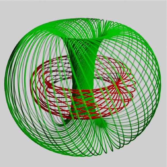
Figure 1.2: Helical spheromak configuration showing two of the magnetic field lines. The original color image from bubbles (under CC-BY 4.0 license) was monochromed.

For both cases we keep the magnetic energy constant while adjust the helicity such that the high helicity case has four times the helicity of the low helicity case. As control cases we also run simulations with no magnetic field and two with only an external field. This gives us seven different simulations.

The stability of the bubble is measured using a coherence measure $d_{\rm mean}$, which is simply the mean distance of the points within the bubble. Weather or not a point belongs to the bubble is determined by the tempearature. All points above a threshold, by definition, belong to it. So, a large value of $d_{\rm mean}$ tells us that the bubble has undergone some significant disruption.

From our calculations (Figure 1.3) we clearly see that a helical internal magnetic field stabilizes the field. This is independent of the type of helical field used (ABC versus spheromak). At a minimum level of helicity we reach stability. If we want the same amount of stability from an external field, however, we require a much larger total magnetic energy content. We estimate that a helical field with maximum strength of the order of ${10}^{-5}\text{\,}\mathrm{G}$ can stabilize the bubble over a time scale of about $250\text{\,}\mathrm{Myr}$. For comparison, these simulations also show that in a purely hydrodynamical case the bubbles can be stable for about $80\text{\,}\mathrm{Myr}$.

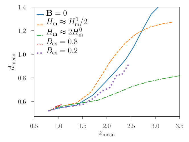
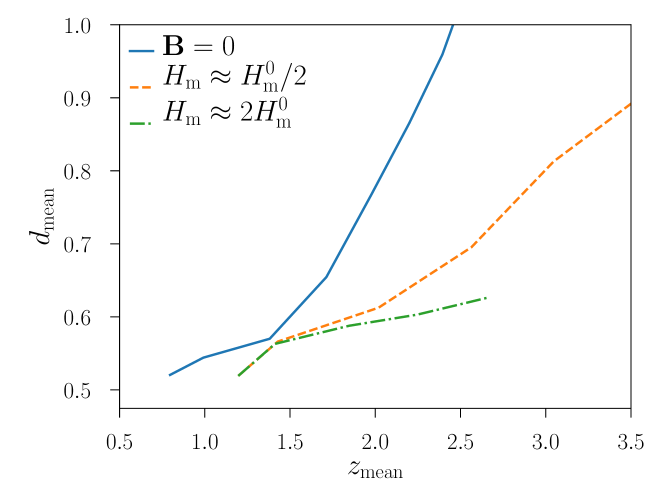
Figure 1.3: Coherence measure $d_{\rm mean}$ of the intergalactic bubbles in dependence of the mean height. The upper panel shows the control case with no magnetic field ($\bm{B}=0$) with the ABC field in two different helicity contents and same energy, and the case of an external magnetic field with strength close to the predicted value for the suppression of the instability on all wave lengths. The lower panel shows the case for the spheromak configuration. The original color figures from bubbles (under CC-BY 4.0 license) were monochromed.

1.8 Conclusions

We have discussed the role of helical magnetic fields in the stabilization of plasmas. First of all we have seen how magnetic helicity is a conserved quantity in ideal MHD and in the high-conductivity limit, that is when magnetic diffusivity is very small. This is the case for various astrophysical plasmas on very different length scales.

Helicity conservation is well illustrated by considering magnetic tubes which are interlocked. Whenever their configuration is characterized by a finite magnetic helicity, it results into a much more stable system than in non-helical cases. On the other hand, the topological linkage of such tubes plays no role in stabilizing the plasma. Therefore, magnetic helicity conservation imposes strong constraints on the relaxation of magnetic fields whenever some helicity is present.

We have discussed helicity conservation in the stability of structures in the solar corona, such as coronal mass ejections, as well as in tokamak fields. On much larger scales, such as galactic and extragalactic environments, we see a similar behavior. In particular, some extragalactic structures moving at high velocity through the extragalactic medium, are observed to be surprisingly stable towards disruption by the Kelvin-Helmoltz instability. Magnetic helicity may, therefore, play an important role against sucha a distruption.

In the last section we have therefore examined the possibility that a helical magnetic field may stabilize extragalactic bubbles even at low magnetic energy densities. These bubbles are observed raising from the midplane of our galaxy and other galaxies into the intergalactic medium. We justify the presence of helicity in these bubbles by the fact the they are boing inflated by an active galactic nucleus or from jets coming from the galactic center, which yield helical fields.

We tested two different types of helical magnetic fields: the ABC flow and a spheromak field. This field initially sits inside the bubble raising through buoyancy in an otherwise stably stratified medium. We quantified the disruption of the bubble and observed that this bubble is stabilized by the helicity towards the Kelvin-Helmholtz instability in the non-linear regime if the magnetic field is sufficiently helical. Our estimate is that a helical field with maximum strength of the order of ${10}^{-5}\text{\,}\mathrm{G}$ can stabilize the bubble over a time scale of at least $250\text{\,}\mathrm{Myr}$, which is more than three times longer than the stability of a non-magnetized bubble. This remarkable example illustrates the role played by magnetic helicity in the stabilization of structures in plasmas. Moreover, it also suggests that helical magnetic fields are present in astrophysical magnetized plasmas wherever stable configurations are observed, and throughout several scales, from stars to extragalactic structures.

References

- Alfvén, (1942) Alfvén, H. (1942). Existence of Electromagnetic-Hydrodynamic Waves. Nature, 150:405–406.
- Arnold, (1986) Arnold, V. I. (1986). The asymptotic hopf invariant and its applications. Sel. Math. Sov., 5:327–345.
- Aschwanden, (2019) Aschwanden, M. J. (2019). Helical twisting number and braiding linkage number of solar coronal loops. Astrophys. J., 874(2):131.
- Batchelor, (1950) Batchelor, G. K. (1950). On the spontaneous magnetic field in a conducting liquid in turbulent motion. Roy. Soc. Lond. Proc. Ser. A, 201:405–416.
- Bekenstein, (1987) Bekenstein, J. D. (1987). Helicity Conservation Laws for Fluids and Plasmas. Astrophys. J., 319:207.
- Bhat et al., (2016) Bhat, P., Subramanian, K., and Brandenburg, A. (2016). A unified large/small-scale dynamo in helical turbulence. Mon. Not. R. Astron. Soc., 461(1):240–247.
- Bîrzan et al., (2004) Bîrzan, L., Rafferty, D. A., McNamara, B. R., Wise, M. W., and Nulsen, P. E. J. (2004). A Systematic Study of Radio-induced X-Ray Cavities in Clusters, Groups, and Galaxies. Astrophys. J., 607(2):800–809.
- Biskamp, (2003) Biskamp, D. (2003). Magnetohydrodynamic Turbulence. Cambridge University Press.
- Bonanno, (2013) Bonanno, A. (2013). Solar Dynamo and Toroidal Field Instabilities. Sol. Phys., 287(1-2):185–196.
- Bonanno et al., (2012) Bonanno, A., Brandenburg, A., Del Sordo, F., and Mitra, D. (2012). Breakdown of chiral symmetry during saturation of the Tayler instability. Phys. Rev. E, 86(1):016313.
- Brandenburg, (2020) Brandenburg, A. (2020). Scientific usage of the pencil code.
- Brandenburg et al., (2009) Brandenburg, A., Candelaresi, S., and Chatterjee, P. (2009). Small-scale magnetic helicity losses from a mean-field dynamo. Mon. Not. R. Astron. Soc., 398:1414–1422.
- Brandenburg and Dobler, (2002) Brandenburg, A. and Dobler, W. (2002). Hydromagnetic turbulence in computer simulations. Computer Physics Communications, 147(1–2):471 – 475. Proceedings of the Europhysics Conference on Computational Physics Computational Modeling and Simulation of Complex Systems.
- Brandenburg and Scannapieco, (2020) Brandenburg, A. and Scannapieco, E. (2020). Magnetic Helicity Dissipation and Production in an Ideal MHD Code. Astrophys. J., 889(1):55.
- Brandenburg and Subramanian, (2005) Brandenburg, A. and Subramanian, K. (2005). Astrophysical magnetic fields and nonlinear dynamo theory. Phys. Rep., 417:1–209.
- Bregman, (1980) Bregman, J. N. (1980). The galactic fountain of high-velocity clouds. Astrophys. J., 236:577–591.
- Candelaresi and Brandenburg, (2011) Candelaresi, S. and Brandenburg, A. (2011). Decay of helical and nonhelical magnetic knots. Phys. Rev. E, 84(1):016406.
- Candelaresi and Del Sordo, (2020) Candelaresi, S. and Del Sordo, F. (2020). Stabilizing Effect of Magnetic Helicity on Magnetic Cavities in the Intergalactic Medium. Astrophys. J., 896(1):86.
- Candelaresi et al., (2021) Candelaresi, S., Hornig, G., Podger, B., and Pontin, D. I. (2021). Topological constraints in the reconnection of vortex braids. Phys. Fluids, 33(5):056101.
- Candelaresi et al., (2014) Candelaresi, S., Pontin, D., and Hornig, G. (2014). Mimetic Methods for Lagrangian Relaxation of Magnetic Fields. SIAM J. Sci. Comput., 36(6):B952–B968.
- Canfield et al., (1999) Canfield, R. C., Hudson, H. S., and McKenzie, D. E. (1999). Sigmoidal morphology and eruptive solar activity. Geophys. Res. Lett., 26:627–630.
- Carilli et al., (1994) Carilli, C. L., Perley, R. A., and Harris, D. E. (1994). Observations of interaction between cluster gas and the radio lobes of cygnus a. Mon. Not. R. Astron. Soc., 270(1):173–177.
- Carilli and Taylor, (2002) Carilli, C. L. and Taylor, G. B. (2002). Cluster magnetic fields. Annu. Rev. Astron. Astr., 40(1):319–348.
- Chamandy, (2016) Chamandy, L. (2016). An analytical dynamo solution for large-scale magnetic fields of galaxies. Mon. Not. R. Astron. Soc., 462(4):4402–4415.
- Chamandy et al., (2014) Chamandy, L., Shukurov, A., Subramanian, K., and Stoker, K. (2014). Non-linear galactic dynamos: a toolbox. Mon. Not. R. Astron. Soc., 443(3):1867–1880.
- Chandrasekhar, (1961) Chandrasekhar, S. (1961). Hydrodynamic and hydromagnetic stability. Oxford Univ. Press.
- Chatterjee et al., (2011) Chatterjee, P., Mitra, D., Brandenburg, A., and Rheinhardt, M. (2011). Spontaneous chiral symmetry breaking by hydromagnetic buoyancy. r, 84(2):025403.
- Cheng et al., (2015) Cheng, K. S., Chernyshov, D. O., Dogiel, V. A., and Ko, C. M. (2015). Multi-wavelength Emission from the Fermi Bubble. II. Secondary Electrons and the Hadronic Model of the Bubble. Astrophys. J., 799(1):112.
- Churazov et al., (2001) Churazov, E., Brüggen, M., Kaiser, C. R., Bohringer, H., and Forman, W. (2001). Evolution of buoyant bubbles in m87. Astrophys. J., 554(1):261–273.
- Craig and Sneyd, (1990) Craig, I. J. D. and Sneyd, A. D. (1990). Nonlinear development of the kink instability in coronal flux tubes. Astrophys. J., 357:653–661.
- Del Sordo et al., (2010) Del Sordo, F., Candelaresi, S., and Brandenburg, A. (2010). Magnetic-field decay of three interlocked flux rings with zero linking number. Phys. Rev. E, 81(3):036401.
- Del Sordo et al., (2013) Del Sordo, F., Guerrero, G., and Brandenburg, A. (2013). Turbulent dynamos with advective magnetic helicity flux. Mon. Not. R. Astron. Soc., 429(2):1686–1694.
- Ebrahimi and Karami, (2016) Ebrahimi, Z. and Karami, K. (2016). Resonant absorption of kink magnetohydrodynamic waves by a magnetic twist in coronal loops. Mon. Not. R. Astron. Soc., 462(1):1002–1011.
- Finkelstein and Weil, (1978) Finkelstein, D. and Weil, D. (1978). Magnetohydrodynamic kinks in astrophysics. Int. J. Theor. Phys., 17(3):201–217.
- Gibson et al., (2002) Gibson, S. E., Fletcher, L., Zanna, G. D., Pike, C. D., Mason, H. E., Mandrini, C. H., Démoulin, P., Gilbert, H., Burkepile, J., Holzer, T., Alexander, D., Liu, Y., Nitta, N., Qiu, J., Schmieder, B., and Thompson, B. J. (2002). The structure and evolution of a sigmoidal active region. Astrophys. J., 574(2):1021.
- Kleeorin et al., (2000) Kleeorin, N., Moss, D., Rogachevskii, I., and Sokoloff, D. (2000). Helicity balance and steady-state strength of the dynamo generated galactic magnetic field. Astron. Astrophys., 361:L5–L8.
- Leka et al., (1996) Leka, K. D., Canfield, R. C., McClymont, A. N., and van Driel-Gesztelyi, L. (1996). Evidence for Current-carrying Emerging Flux. Astrophys. J., 462:547.
- McNamara and Nulsen, (2007) McNamara, B. and Nulsen, P. (2007). Heating hot atmospheres with active galactic nuclei. Annu. Rev. Astron. Astr., 45(1):117–175.
- Montmerle, (2011) Montmerle, T. (2011). Galactic and extragalactic hot bubbles: Feedback from massive stars. In Charbonnel, C. and Montmerle, T., editors, EAS Publications Series, volume 51 of EAS Publications Series, pages 299–310.
- Ntormousi et al., (2020) Ntormousi, E., Tassis, K., Del Sordo, F., Fragkoudi, F., and Pakmor, R. (2020). A dynamo amplifying the magnetic field of a Milky-Way-like galaxy. Astron. Astrophys., 641:A165.
- Priest and Forbes, (2000) Priest, E. R. and Forbes, T. G. (2000). Magnetic reconnection: MHD theory and applications.
- (42) Prior, C. and Yeates, A. R. (2016a). Twisted versus braided magnetic flux ropes in coronal geometry. I. Construction and relaxation. Astron. Astrophys., 587:A125.
- (43) Prior, C. and Yeates, A. R. (2016b). Twisted versus braided magnetic flux ropes in coronal geometry. II. Comparative behaviour. Astron. Astrophys., 591:A16.
- Rincon, (2021) Rincon, F. (2021). Helical turbulent nonlinear dynamo at large magnetic Reynolds numbers. arXiv e-prints, page arXiv:2108.12037.
- Rust and Kumar, (1996) Rust, D. M. and Kumar, A. (1996). Evidence for Helically Kinked Magnetic Flux Ropes in Solar Eruptions. Astrophys. J.l, 464:L199.
- Shukurov et al., (2008) Shukurov, A., Sokoloff, D., Subramanian, K., and Brandenburg, A. (2008). Galactic dynamo and helicity losses through fountain flow. Astron. Astrophys., 448:L33–L36.
- Sur et al., (2007) Sur, S., Shukurov, A., and Subramanian, K. (2007). Galactic dynamos supported by magnetic helicity fluxes. Mon. Not. R. Astron. Soc., 377:874–882.
- Taylor et al., (2002) Taylor, G. B., Fabian, A. C., and Allen, S. W. (2002). Magnetic fields in the Centaurus cluster. Mon. Not. R. Astron. Soc., 334(4):769–776.
- Taylor, (1974) Taylor, J. B. (1974). Relaxation of toroidal plasma and generation of reverse magnetic fields. Phys. Rev. Lett., 33:1139–1141.
- Taylor, (1986) Taylor, J. B. (1986). Relaxation and magnetic reconnection in plasmas. Rev. Mod. Phys., 58:741–763.
- Vemareddy et al., (2017) Vemareddy, P., Gopalswamy, N., and Ravindra, B. (2017). Prominence eruption initiated by helical kink instability of an embedded flux rope. Astrophys. J., 850(1):38.
- Wang et al., (2016) Wang, R., Liu, Y. D., Wiegelmann, T., Cheng, X., Hu, H., and Yang, Z. (2016). Relationship between sunspot rotation and a major solar eruption on 12 july 2012. Sol. Phys., pages 1–13.
- Woltjer, (1958) Woltjer, L. (1958). A theorem on force-free magnetic fields. Proc. Nat. Acad. Sci. USA, 44:489–491.
- Yeates et al., (2010) Yeates, A. R., Hornig, G., and Wilmot-Smith, A. L. (2010). Topological constraints on magnetic relaxation. Phys. Rev. Lett., 105(8):085002.