Computing Class Hierarchies from Classifiers

Abstract

A class or taxonomic hierarchy is often manually constructed, and part of our knowledge about the world. In this paper, we propose a novel algorithm for automatically acquiring a class hierarchy from a classifier which is often a large neural network these days. The information that we need from a classifier is its confusion matrix which contains, for each pair of base classes, the number of errors the classifier makes by mistaking one for another. Our algorithm produces surprisingly good hierarchies for some well-known deep neural network models trained on the CIFAR-10 dataset, a neural network model for predicting the native language of a non-native English speaker, a neural network model for detecting the language of a written text, and a classifier for identifying music genre. In the literature, such class hierarchies have been used to provide interpretability to the neural networks. We also discuss some other potential uses of the acquired hierarchies.

Introduction

Much of our knowledge about the world is organized hierarchically. We have classes or concepts like chairs, tables, office furniture, plastic furniture, furniture, and so on. Similarly, we may classify animals into cats, dogs, mountain lions, small dogs, pets, and so on. Many, if not most, of these concepts are not precisely defined, and are classified by features like their functionality and their visual appearance to us. With the advance of deep learning, we now have computer programs that can recognise many of these classes with an accuracy that rivals human perception. However, these programs are often flat and end-to-end, in the sense that they just classify the input into a class without referencing to any possible hierarchies among these classes.

There has been work on leveraging our knowledge about class hierarchies to improve the performance of deep neural network classification models in terms of accuracies, and sampling and training efficiencies (Brust and Denzler 2019; Marszalek and Schmid 2007; Gao and Koller 2011; Li et al. 2019; Pan and Shen 2020). In this paper, our goal is somewhat the opposite. We take a good classification model as a given black box, and try to derive from it a plausible class hierarchy network. Our basic assumption is that the classification model is accurate enough so that the “closeness” or “relatedness” of two classes are directly related to how often the model misclassifies one of them as the other.

We can see several potential uses of a class hierarchy constructed from a classification model. Firstly, the derived class hierarchy can be used as a sort of justification or explanation of the given classification model, as some previous work (Frosst and Hinton 2017; Wan et al. 2021) has argued. Secondly, a good class hierarchy is useful in its own right. For example, given a good model to identify the native language of a non-native English speaker, we can construct a hierarchy of languages that can help to group non-native English speakers for the purpose of teaching English as a foreign language. We will give several examples of this nature when discussing experiments of this work.

As we mentioned earlier, our knowledge about the world is often organized hierarchically. Thus coming up with a good class hierarchy can be considered a part of scientific discovery. Hopefully our proposed algorithm for acquiring such knowledge from an accurate neural network classification model can contribute to this process of scientific discovery.

This rest of this paper is organized as follows. In the next section, we describe the formal setup of the problem and give our method for solving it. We then show two intuitive properties of our algorithm. Next we apply our algorithm to several domains, and discuss our expeperimental results. We then discuss related work and conclude the paper.

Our Method

Throughout this paper, we use numerical numbers starting at $0$ to denote base classes. Given a set $C$ of $n$ base classes $\{0,...,{n-1}\}$, we consider ways to organize them into a hierarchy. In graph theoretic terms, a class hierarchy is a labeled tree where the label of a node is the class that the node represents, and the parent to children edges stand for subsumption. So if $N$ is a child node of $N^{\prime}$, then the class represented by node $N$ is a subclass of that represented by $N^{\prime}$. Thus for a tree to be a class hierarchy for $C$, its leaves must be labeled by base classes in $C$, and its internal nodes by classes not in $C$. While every class in $C$ must be a label of a leave, it can be the labels of multiple leaves. If a class tree has no distinct nodes labeled by the same class, then there is no overlapping between any of its subclasses. In this case, we call the class tree a Single Inheritance Tree (SIT) as there is a unique path from the root class to any of its subclasses. Otherwise, it is called a Multiple Inheritance Tree (MIT). The following example illustrates the difference between these two types of hierarchies. Consider $C=\{0,1,2\}$ with $0$ for cat, $1$ for dog, and $2$ for tiger. The class $cat$ is related to both $dog$ and $tiger$. A reasonable way to take account of this is to create a super class for $cat$ and $dog$, and another for $cat$ and $tiger$. This will yield a MIT as shown in Figure 1. On the other hand, if we insist on using a SIT, and assume that $cat$ is closer to $dog$, we may come up with the SIT as shown in Figure 1.

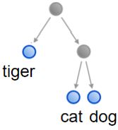
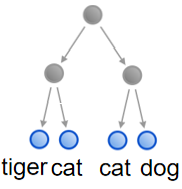
Figure 1: (a) A single inheritance tree; (b) A multiple inheritance tree

We propose an iterative algorithm to construct a hierarchy for a given set of base classes by first merging some base classes into super-classes, and then iteratively merging the remaining base classes and the new classes into more general classes until a single most general class is obtained. The general idea is that classes are merged into a new class if and only if they have similar properties. The question is of course how to define similarity. For this, we will use a similarity matrix that measures the degree of similarities between any two classes, and an adjustable threshold to define whether the degrees of similarity between two classes are large enough to be merged into a new class.

To compute the degree of similarities between two classes, we assume a classification model for the base classes. It can be a decision tree, a neuron network, a set of rules or others. The only thing we need from the model is its so called confusion matrix (Fawcett 2006): the confusion matrix ${\mathbf{M}}$ of a model for $n$ classes is a $n\times n$ integer matrix where for any $0\leq i,j\leq n-1$, the element ${\mathbf{M}}_{ij}$ is the number of samples in the testing set that are labeled as class $i$ but classified as class $j$ by the model. Often, the sample set is not balanced, so we use a normalized version of the confusion matrix. Specifically, if ${\mathbf{M}}$ is a confusion matrix, then its normalized version, written $\widehat{{\mathbf{M}}}$, is defined as: for each $0\leq i,j\leq n-1$,

$$\widehat{{\mathbf{M}}}_{ij}=\frac{{\mathbf{M}}_{ij}}{\sum^{n-1}_{k=0}{\mathbf{M}}_{ik}}.$$

Notice that $\sum^{n-1}_{k=0}{\mathbf{M}}_{ik}$ is the total number of class $i$ instances used to test the classifier to derive the confusion matrix. So $\widehat{{\mathbf{M}}}_{ij}$ is in fact the error rate of the model for confusing class $i$ instances as class $j$’s, and our normalized confusion matrix can be called the confusion rate matrix.

A confusion matrix is often not symmetric in the sense that for many $i$ and $j$, ${\mathbf{M}}_{ij}\neq{\mathbf{M}}_{ji}$, meaning the number of class $i$ instances that are mis-classified as class $j$ is not equal to the number of class $j$ instances that are mis-classified as class $i$. However, for the purpose of class hierarchy, we want a number to measure the similarity of two classes, and this number should be symmetric. This leads to our following definition of similarity matrices.

Definition 1

The similarity matrix ${\mathbf{S}}$ of a classifier is

$$\mathbf{S}=\frac{1}{2}(\widehat{{\mathbf{M}}}+\widehat{{\mathbf{M}}}^{T}),$$

where $\widehat{{\mathbf{M}}}$ is the normalized confusion matrix of the classifier.

Intuitively, ${\mathbf{S}}_{ij}=\frac{1}{2}(\widehat{{\mathbf{M}}}_{ij}+\widehat{{\mathbf{M}}}_{ji})$ is the average confusion rate between classes $i$ and $j$, and the higher it is, the more similar the classes $i$ and $j$ are, and more likely they are related and inherited from a common ancestor. But it is domain dependent that just how large the value ${\mathbf{S}}_{ij}$ should be to trigger the decision that they are likely siblings and thus should be merged to form a superclass. To account for this, we introduce a threshold ratio $r$, and merge classes $i$ and $j$ if the following condition holds:

$${\mathbf{S}}_{ij}>0\textbf{ and }{\mathbf{S}}_{ij}+\delta\geq\max(\{{\mathbf{S}}_{i,k}|k\neq i\}\cup\{{\mathbf{S}}_{j,k}|k\neq j\})$$ (1)

where $\delta=r*m=r*\max\{{\mathbf{S}}_{i,j}|0\leq i<j\leq n-1\}$. It is possible that a class may need to be merged with two other classes. In this case, three of them will be merged. This means that our computed class hierarchy may not be a binary tree.

The condition (1) will apply not only to base classes but also to newly created superclasses, with a more involved definition for $m$ to compute the $\delta$. This implies that we will need a way to compute the similarity scores between pairs of superclasses created during the process of constructing a hierarchy. This can be computed from the scores between the superclasses’ subclasses by taking the min, the max, the average, or using some other formulas. Intuitively, taking the min is a conservative approach, the max aggressive, and the average in the middle. However, by choosing an appropriate threshold ratio $r$ mentioned earlier, we can twist the middle approach to make it either more conservative or more aggressive. So in this paper when computing the similarity between two classes, we take the average of the similarity scores between their subclasses. Indeed, as we shall see, it works well for the domains that we have tried so far.

Figure 5 outlines our algorithm for computing a class hierarchy given the similarity matrix of a classifier. The main function is $CH({\mathbf{S}},r,flag)$, which takes ${\mathbf{S}}$, the similarity matrix of the classifier defined earlier, $r\geq 0$, the threshold ratio $r$ mentioned above, and $flag$, a boolean number to indicate whether the returned class hierarchy must be of single inheritance. It initializes $\widehat{\mathbf{S}}$ to ${\mathbf{S}}$, and $H$ to $\{t_{0},...,t_{n-1}\}$, where $t_{i}$ is the singleton tree for base class $i$. It then loops through $MERGE(H,\widehat{\mathbf{S}},\delta,flag)$, which merges some classes in $H$ to create some new superclasses, and $SIMILARITY(H,\widehat{\mathbf{S}})$, which computes a new similarity matrix for the new set $H$ of classes. Notice that we identify a tree in $H$ with the class denoted by its root. The loop exits when $MERGE()$ does not produce any new class, either because the current $H$ contains just one tree or none of the trees in $H$ can be merged. In the former case, the tree in $H$ is then returned as the computed hierarchy. In the latter case, all trees in $H$ are combined to form a single tree.

Notice that $m$ for computing $\delta$ in $CH()$ is initialized first for base classes. It is then updated (line 8) by taking the maximum of similarity scores other than those with overlapping subtrees. Nodes with overlapping subtrees can indeed be generated when computing MITs. The similarity scores between these nodes will be close to large, often close to 1 like ${\mathbf{S}}_{ii}$, so should be excluded when computing the threshold $\delta$.

Both $SIMILARITY()$ and $MERGE()$ functions are sketched in Figure 5. Crucially, $FIND\_ALL\_PAIRS()$ returns a list of all pairs of class indices $(i,j)$ that satisfy condition (1), and this list is passed to $PAIRS\_TO\_GRAPHS()$ to return a partition of $H$, with each set in the partition representing the set of classes that are to be merged into a superclass. The complete code of our algorithm is given in an appendix uploaded as supplementary material.

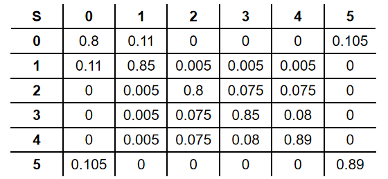
Figure 2: A similarity matrix demo.

To illustrate, consider a case with 6 base classes and a confusion matrix that produces the initial similarity matrix given in Figure 2. Initially $H=\{t_{0},..,t_{5}\}$. $MERGE()$ uses condition (1) to decide which trees (classes) in $H$ are to be merged. Suppose we let $r=0.1$. Then

$$m=\max(\{{\mathbf{S}}_{i,j}|0\leq i<j\leq n-1\})=0.11$$

$$\delta=r*m=0.011$$

So by (1), the pairs in the following list could be merged:

$$[(t_{0},t_{1}),(t_{0},t_{5}),(t_{3},t_{4}),(t_{2},t_{3}),(t_{2},t_{4})].$$

We see that some of these pairs have common elements so a decision needs to be made whether to further merge them. In this case, our algorithm will merge $(t_{3},t_{4}),(t_{2},t_{3}),(t_{2},t_{4})$ into $(t_{2},t_{3},t_{4})$, thus creating a new tree with three children trees $t_{2}$, $t_{3}$ and $t_{4}$. However, it won’t merge $(t_{0},t_{1})$ and $(t_{0},t_{5})$ into $(t_{0},t_{1},t_{5})$ because the pair $(t_{1},t_{5})$ is not in the above list as classes $1$ and $5$ are not similar enough.

If SIT is desired, the above pair list will be converted into $[(t_{0},t_{1}),(t_{2},t_{3},t_{4})]$. Notice that while both $(t_{0},t_{5})$ and $(t_{0},t_{1})$ are in the above list, only the latter is selected as ${\mathbf{S}_{01}}>{\mathbf{S}_{05}}$, meaning class $0$ is more similar to class $1$ than class $5$.

So $H$ will be updated to be the following set of trees $\{t_{01},t_{234},t_{5}\}$, and its similarity matrix computed as given in Figure 3. Next step is to combine $(t_{01},t_{5})$ to get $t_{01\_5}$, and then combine it with $t_{234}$ to return the tree as shown in Figure 4.

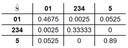
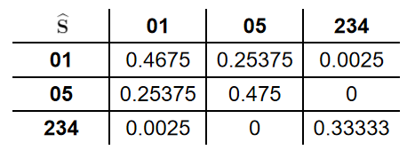
Figure 3: Updated similarity matrix: (a) SIT, and (b) MIT

However, if MIT is required, the pair list will be converted into $[(t_{0},t_{1}),(t_{0},t_{5}),(t_{2},t_{3},t_{4})]$, both of two pairs related to $t_{0}$ will be saved because overlapping is allowed. Then the $H$ will be updated to $\{t_{01},t_{05},t_{234}\}$. The new similarity matrix will be figure 3. At next iteration, $(t_{01},t_{05})$ will be combined and get a new superclass $t_{01\_05}$ then it will be combined with $t_{234}$ to obtain the tree as shown in Figure 4.

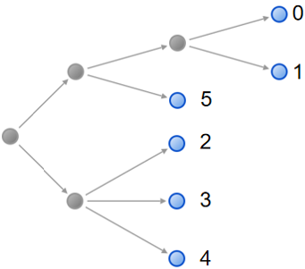
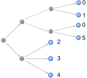
Figure 4: Hierarchies for $\mathbf{S}$ in Figure 2: (a) SIT; (b) MIT

1:${\mathbf{S}}$ - similarity matrix; $r$ - threshold ratio, a non-negative real for calculating clustering sensitivity; $flag$ - 1 if the output must be of single inheritance, 0 otherwise.

2:a class hierarchy for $C$.

3:function CH(${\mathbf{S}},r,flag$) (main function)

4:     $H=\{t_{0},...,t_{n-1}\}$

5:     ${\widehat{\mathbf{S}}}={\mathbf{S}}$

6:     $m=\max(\{\widehat{{\mathbf{S}}}_{i,j}|0\leq i<j\leq n-1\})$

7:     while $len(H)>1$ and $m>0$ do

8:         $H=\textsc{merge}(H,\widehat{{\mathbf{S}}},r*m,flag)$

9:         $\widehat{{\mathbf{S}}}=\textsc{similarity}(H,\widehat{{\mathbf{S}}})$

10:         $m=\max\{\widehat{{\mathbf{S}}}_{i,j}$ for all $0\leq i<j<len(H)$ such that $H[i]$ and $H[j]$ has no overlap$\}$ or $0$      

11:     if $len(H)>1$ then

12:         $H=$ Combine all trees in $H$      

13:     return $H$

1:Tree set: $H$, similarity matrix: $\widehat{{\mathbf{S}}}$, threshold: $\delta$, tree type flag: $flag$.

2:Updated tree set $H$.

3:function Merge($H,\widehat{{\mathbf{S}}},\delta,flag$)

4:     $P=\textsc{Find\_all\_pairs}(\widehat{{\mathbf{S}}},\delta)$

5:     $G=\textsc{pairs\_to\_graphs}(\widehat{{\mathbf{S}}},P,flag)$

6:     $H^{\prime}\leftarrow[]$

7:     $rest\leftarrow[0]*len(H)$

8:     for $graph$ in $G$ do

9:         $tree\leftarrow$ Combine trees indicated by $graph$.

10:         $H^{\prime}.append(tree)$

11:         for $i$ in $graph$ do

12:              $rest[i]=1$               

13:     for $i$ in $range(len(H))$ do

14:         if $rest[i]==0$ then

15:              $H^{\prime}.append(H[i])$               

16:     return $H^{\prime}$

1:Tree set: $H$, similarity matrix: $\widehat{{\mathbf{S}}}$.

2:Updated similarity matrix $\widehat{{\mathbf{S}}}$.

3:function Similarity($H,\widehat{{\mathbf{S}}}$)

4:     $n\leftarrow len(H)$

5:     $\widehat{{\mathbf{S}}}^{\prime}\leftarrow n\times n$ empty matrix

6:     for $i$ in $range(n)$ do

7:         $A\leftarrow$ children index group of $H[i]$

8:         for $j$ in $range(n)$ do

9:              $B\leftarrow$ children index group of $H[j]$

10:              $\widehat{{\mathbf{S}}}^{\prime}_{ij}\leftarrow avg(\{\widehat{{\mathbf{S}}}_{ab}|a\in A,b\in B\})$               

11:     return $\widehat{{\mathbf{S}}}^{\prime}$

Figure 5: Computing Class Hierarchies

Some Properties

The following simple property says that when the given classification model has the same similarity score for all pairs of base classes, then the computed hierarchy simply groups all base classes into a superclass as the classifier is equally confused about each pairs of them.

Property 1

If all the non-diagonal elements of $\mathbf{S}$ are the same, then for any $r$ and $flag$, $CH({\mathbf{S}},r,flag)$ returns a tree that has all the base classes as the children of the root.

To state the next property, we introduce a notion of islands. Given a similarity matrix $\mathbf{S}$ for a set $C=\{0,...,{n-1}\}$ of classes, we say that a proper subset $X$ of $C$ is an island (under $\mathbf{S}$) if for any $i$ in $X$ and $j$ in $C\setminus X$, ${\mathbf{S}}_{ij}=0$, and for any $i$ in X, there is another $j$ in $X$ such that $i\neq j$ and ${\mathbf{S}}_{ij}\neq 0$.

It is easy to see that for a given similarity matrix, there may not exist an island. Furthermore, if $X$ and $Y$ are two distinct islands, then $X\cap Y=\emptyset$. This means that either $C$ has no island or there is a partition $\{X_{1},...,X_{k}\}$, $k>1$, of $C$ such that each $X_{i}$ is an island of $C$.

Property 2

If $C$ has an island under ${\mathbf{S}}$, then there is a partition $\{X_{1},...,X_{k}\}$, $k>1$, of $C$ such that each $X_{i}$ is an island of $C$, and for any $r$ and $flag$, $CH({\mathbf{S}},r,flag)$ returns a tree whose root has $k$ children $t_{1},...,t_{k}$ such that the set of leaves in $t_{i}$ is $X_{i}$, $1\leq i\leq k$.

This property means that, for an island, its class hierarchy can be constructed on its own independent of other classes, and when a set of classes is partitioned into a collection of islands, the final hierarchy is just a superclass with each of the island as a direct subclass.

Notice that as a special case, if a base class $i$ by itself is an island, then the given model classifies it perfectly and our computed hierarchy will always put it directly under the root.

The basic idea behind our proof of this property is that suppose $X$ is an island, then according to our algorithm, during the construction of a hierarchy, for any two trees $t$ and $t^{\prime}$, if the leaves in $t$ are all from $X$ and none of the leaves in $t^{\prime}$ are from $X$, then the similarity score between these two trees will be 0.

These two properties are useful to have but are by no means complete. It’s an interesting open theoretical question if there is a complete set of properties that captures our algorithm in the sense that any algorithm that satisfies the set of properties will be equivalent to ours.

Experiments

The key question that we had when starting this project was how good a class hierarchy can one compute based on only a confusion matrix about a classifier. In the end, we were pleasantly surprised that our algorithm came out with very informative ones. We describe in this section the results of applying our algorithm in Figure 5 to the following classification tasks and models:

• Two well-known models ResNet10 (He et al. 2016) and WideResNet28 (Zagoruyko and Komodakis 2016) for CIFAR-10 (Krizhevsky, Hinton et al. 2009) image classification task.

• Two models for two natural language classification tasks, one based on speech and the other on texts.

• A model for a music genre classification task based on music spectrogram.

In our experiment with these applications, we choose the threshold ratio $r=0.1$ or $r=0.05$. The smaller $r$ is, the more conservative our algorithm is when deciding when to merge two classes. To give an idea of how different values of $r$ affect the outcome, we include the results of using $r=0,0.1,0.2,0.3,0.8,\geq 1$ on the WideResNet28 model for CIFAR-10 in the supplementary material.

Image Classification

CIFAR-10 is a widely used dataset for machine learning and computer vision. It contains 6000 images for each of the following 10 base classes: airplanes, cars, birds, cats, deer, dogs, frogs, horses, ships, and trucks. We considered two well-known CNNs, ResNet10 and WideResNet28, on the CIFAR-10 dataset. Their accuracies are 93.64% and 97.61%, respectively. Figure 6 shows the SITs (single inheritance trees) returned by our algorithm on them with $r=0.1$ ($flag=1$). As for the MITs for these two models, they have little differences with SITs in this task when $r=0.1$. More specifically, the MIT is the same with SIT for WideResNet28 model.

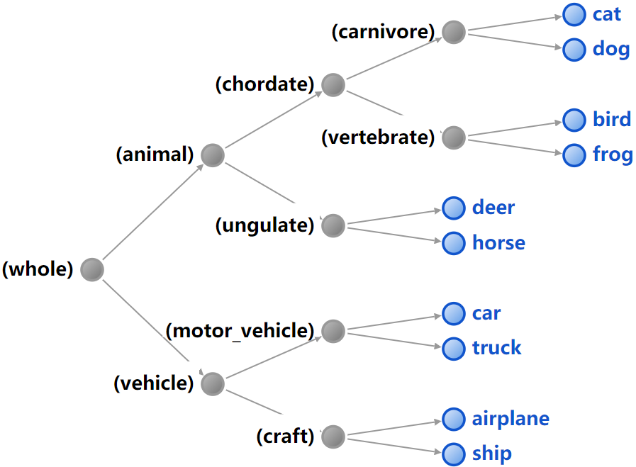
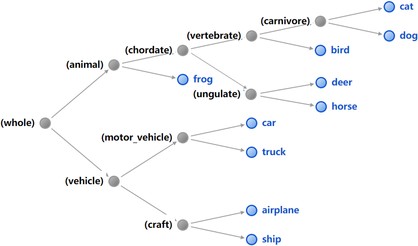
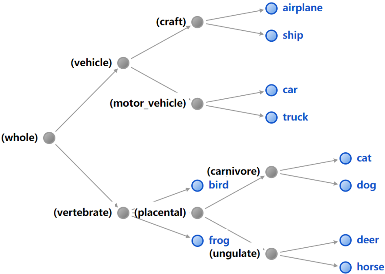
Figure 6: The generated class hierarchy of ResNet10 (a) and WideResNet28 (b), and WordNet (c) hierarchy on CIFAR-10. For ease of comparison, the lables of internal nodes are in paranthesis and obtained by searching the first common ancestor of each sub-tree’s leaves from WordNet concept trees.

One can see that these two hierarchies are close, with major difference on the class “frog”. In the ResNet10 model, “frog” and “bird” have a confusion number high enough to be combined into a superclass. However, under the WideResNet28 model, “frog” is well separated from other “chordates”.

Notice that the closeness of the SITs for the two models is despite the fact that one of them has much higher accuracy than the other. This shows the robustness of our algorithm, and also indicates that the resulting SITs are indeed “correct”.

Notice that ResNet10 and WideResNet28 are classification models based on images. Since WordNet includes conceptual-semantic relations between English words, one can also use it to construct a hierarchy of the 10 classes using their English labels. The idea is that given a set of concepts in WordNet, one can find a most specific class that subsumes these concepts. Figure 6 is the hierarchy obtained this way for CIFAR-10 classes using WordNet. We can see that all three hierarchies have the same structure for the following 8 classes: airplanes, cars, cats, deer, dogs, horses, ships, and trucks. For the remaining two, birds and frogs, the hierarchy computed from WideResNet28 is closer to the one from WordNet. It is certainly reassuring that the class hierarchies that are computed by our algorithm using image-based classification models turn out to be similar with the concept hierarchy in a human maintained database of conceptual-semantic relations.

Besides the pre-existing WordNet hierarchy, there has also been work on generating class hierarchies by using some features inside a classification model. A recent work by Wan et al. (2021) proposes a method that takes the weights of the last full-connection neural layer as the feature embeddings of the classes, and use them to construct a class hierarchy, which they called it a Neural-Backed Decision Tree (NBDT). They claimed that such NBDTs can improve both the accuracy and interpretability of the original model.

Figure 7 is the NBDT from (Wan et al. 2021) using the ResNet10 model. For the WideResNet28 model, their NBDT turns out to be the same as Figure 6, the hierarchy computed by our algorithm using the ResNet10 model. So our algorithm generates the same hierarchy using a less accurate model. Furthermore, considering that our algorithm treats a model like ResNet10 as blackbox while the algorithm in (Wan et al. 2021) uses weights inside a neural network, this result is definitely unexpected and a pleasant surprise!

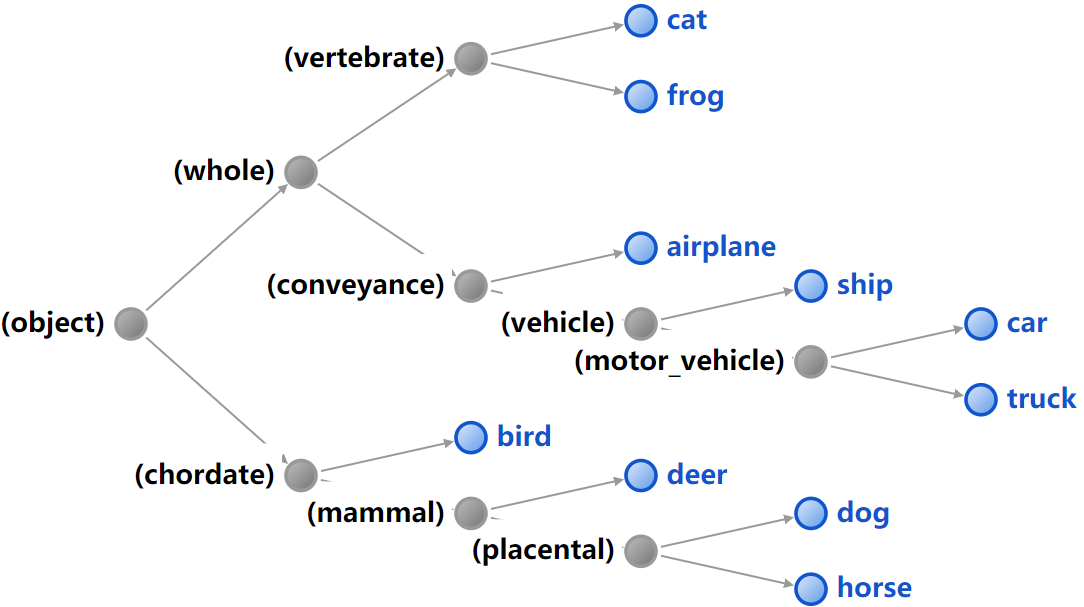
Figure 7: The NBDT induced by ResNet10.

Wan et al. (2021) proposed a new loss function based on their NBDTs to finetune the model and showed that this sometimes can improve the accuracy of the original neural network. In order to compare the hierarchies, we just replaced their NBDTs with our generated hierarchies (SITs) and finetuned the model to obtain our performance. For CIFAR-10 and CIFAR-100, Table 1 shows the accuracies of ResNet10, ResNet18, WideResNet28, as well as their revised models obtained by applying NBDTs and SITs. Except for ResNet18 on CIFAR-100, using our generated hierarchies actually produce a slight boost.

Method	Backbone	CIFAR-10	CIFAR-100
NN	resnet10	93.64	73.66
NN+SIT (ours)	resnet10	93.78	73.74
NN	resnet18	94.74	75.92
NN+NBDT	resnet18	94.82	77.09
NN+SIT (ours)	resnet18	95.03	76.16
NN	wrn28	97.62	82.09
NN+NBDT	wrn28	97.55	82.97
NN+SIT (ours)	wrn28	97.71	83.22

Table 1: The performance comparison of the original neural networks (NN), NN with their induced NBDTs (NN+NBDT) and NN with our generated hierarchis (NN+SIT). Wrn28 represents WideResNet28 model. (Wan et al. 2021) didn’t provide their results on resnet10.

Native Language Identification

Our next experiment uses models for natural language classification. We consider two models, one for identifying the speaker’s native language from their English speech, and the other for detecting the language given a text input.

The first model is by Rama and Çöltekin (2017). They built an LDA-based classifier for detecting the speaker’s native language from the recordings of their English speech. The native languages considered are Arabic (ARA), Chinese (CHI), French (FRE), German (GER), Hindi (HIN), Italian (ITA), Japanese (JPN), Korean (KOR), Spanish (SPA), Telugu (TEL), and Turkish (TUR). Figure 8 shows the SIT and MIT generated from the confusion matrix of this model. In both hierarchies, Hindi and Telugu, which are two languages in India, are grouped together. Chinese, Japanese, and Korean are in a separate branch from other languages. The main difference between the SIT and MIT is that in the MIT, Turkish is duplicated once and combined with Arabic, which seems to make more sense.

One possible use of the class hierarchies is in the teaching of English as a second language. The hypothesis is that people whose native languages are closer according to the hierarchy are likely to have some common issues when learning English and thus may be better to be in the same class if necessary.

These experiments showed that our proposed algorithm can generate a very proper hierarchy which could also be used to help to group non-native English speakers for the purpose of teaching English as a foreign language.

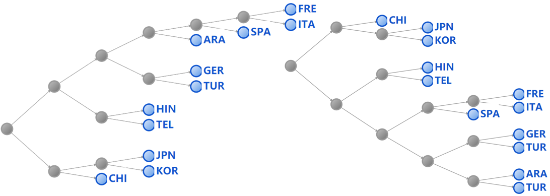
Figure 8: The generated class hierarchies for native language identification with speech as input with $r=0.05$ for both SIT (left) and MIT (right).

The second model that we considered is the one by Simoes, Almeida, and Byers (2014). They built a neural network to detect the language of a text. The considered six Latin languages: English, German, Spanish, French, Portuguese, and Italian. Figure 9 shows the SIT computed by our algorithm using the confusion matrix of the model with $r=0.05$. We see the hierarchy groups German and English in one branch and the rest the other. In fact, German and English belong to what is called Germanic languages (Wikipedia contributors 2021a) , and the rest Romance languages. Again, it was a pleasant surprise to us that our fully automatic algorithm for building a class hierarchy based only on the confusion matrix of a model somehow made the correct classification. Of course, one can also say that this means the model by Simoes, Almeida, and Byers (2014) is really good.

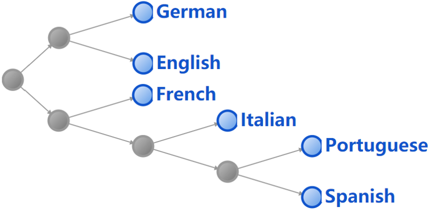
Figure 9: SIT for language identification task with text as input with $r=0.05$.

Music Genre Classification

Our next application is on music genre classification and the model is from Senac et al. (2017). It is a CNN model to classify the genre of the music based on its spectrogram. Figure 10 is the hierarchy generated from the confusion matrix of this model. It is interesting to see that it groups classical music and jazz together. This means that in terms of spectrogram, classical music and jazz are more similar than others. Indeed, according to the current Wikipedia jazz entry (Wikipedia contributors 2021b), “Jazz originated in the late-19th to early-20th century as interpretations of American and European classical music entwined with African and slave folk songs and the influences of West African culture”.

Assuming that people who like one type of music will likely like another type of music with similar spectrogram, our generated hierarchy can be used for music recommendation. For example, a music service can recommend blues to someone who listens to a lot of country music, and vice versa.

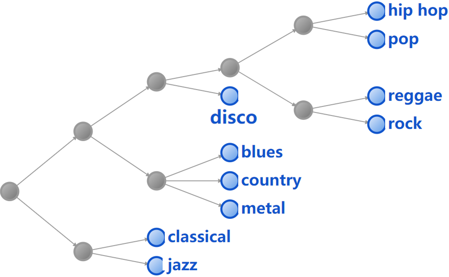
Figure 10: SIT for music genre classification task with $r=0.05$.

Related Works

Class hierarchies are widely used to organize human knowledge about concepts. So it is not surprising there has been much work on utilizing this knowledge in AI. For instance, in machine learning, utilizing word/concept hierarchies derived from the lexical database WordNet, Marszalek and Schmid (2007) considered integrating prior knowledge about relationships among classes into the visual appearance learning. Gao and Koller (2011) applied a set of binary classifiers at each node of the hierarchy structure to achieve a good trade-off between accuracy and speed. Brust and Denzler (2019) integrates additional domain knowledge into classification and converted the properties of the hierarchy into a probabilistic model to improve existing classifiers.

Somewhat related is work on learning a decision tree from data (Quinlan 1983). More recently instead of raw data, Wan et al. (2021) considered constructing a decision tree from the weights of the last full-connection layer, and called it a Neural-Backed Decision Tree (NBDT). We have compared their NBDTs with our hierarchies on the two CIFAR-10 models. In terms of algorithms, they used the hierarchical agglomerative clustering algorithm from (Ward Jr 1963). This is an efficient clustering algorithm that has been widely used in fields about document clustering (Zhao, Karypis, and Fayyad 2005), multiple sequence alignment (Corpet 1988) and air pollution analysis (Govender and Sivakumar 2020). It constructs a binary tree starting from input data as leaves and merging a pair of nodes step by step until only one node is left, which represents the entire data set. Our algorithm shares this bottom up approach. However, our algorithm is not restricted to binary trees, allows multiple inheritance, and can be fine-tuned by the threshold ratio $r$.

Similar to our work, Xiong (2012); Cavalin and Oliveira (2018) also use a model’s confusion matrix to build a class hierarchy. However, their algorithms are significantly different from ours. Cavalin and Oliveira (2018) used the following Euclidean Distance (ED) to measure the distance between two classes:

$\sqrt{\sum_{k=0}^{n-1}({\mathbf{M}}_{ik}-{\mathbf{M}}_{jk})^{2}}$

Their idea is that if a model has similar prediction distribution on $i$ and $j$, then the two classes should be very close. Also using prediction distribution, but instead of Euclidean distance, Xiong (2012) used the sum of absolute difference between two classes:

$$\sum_{k=0}^{n-1}|{\mathbf{M}}_{ik}-{\mathbf{M}}_{jk}|.$$

Instead of using a fixed matrix, our algorithm uses a dynamic criteria based on constraint (1). As an example to illustrate the differences, Figure 11 shows the hierarchy generated using the algorithm in (Cavalin and Oliveira 2018) on the ResNet10 model for CIFAR-10. It is hard to justify such a hierarchy.

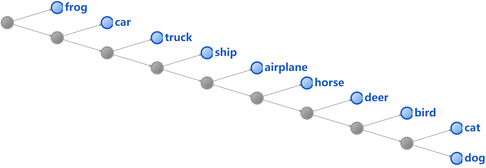
Figure 11: The hierarchy generated using Euclidean Distance on the ResNet10 model for CIFAR-10

Conclusion

We have proposed an algorithm for computing a class hierarchy from a classification model. Our algorithm treats the model as a black box, and uses only its so-called confusion matrix - the matrix that records the number of errors that the model makes by misclassifying one class as another. It generates surprisingly good hierarchies in a number of domains. For CIFAR-10, it even generates the same hierarchy using ResNet10 as the neural-backed decision tree of (Wan et al. 2021) using WideResNet28, despite that ResNet10 is not as accurate as WideResNet28, and that we use only the confusion matrix while they used parameters inside a neural network.

We believe this work provides an interesting new direction for connecting black box classification models which are often large neural networks and symbolic knowledge. For us, future work includes using computed class hierarchies during the training process, as well as applying our algorithm for scientific discovery in some large sets of classes for which there are still not good class hierarchies but enough data to train some reasonably accurate classification models.

Appendix

This supplementary material includes two subsections. First is the detailed codes for functions we used in the $MERGE()$ function. The second subsection is to explore how important of parameter $r$ is to the generated hierarchies.

Algorithms Codes

The detailed codes for function $FIND\_ALL\_PAIRS()$ are shown in figure 12. It found all pairs satisfying condition

$${\mathbf{S}}_{ij}>0\textbf{ and }{\mathbf{S}}_{ij}+\delta\geq\max(\{{\mathbf{S}}_{i,k}|k\neq i\}\cup\{{\mathbf{S}}_{j,k}|k\neq j\})$$ (2)

which we mentioned before and sorted them based on their similarity scores so that later the pair with higher score will be dealt earlier at every iteration.

1:$\widehat{{\mathbf{S}}}$ - similarity matrix. $\delta$ - similarity threshold.

2:$P$ - a list which includes the pair needs to be cared.

3:function find_all_pairs($\widehat{{\mathbf{S}}},\delta$)

4:     $N\leftarrow len(\widehat{{\mathbf{S}}})$

5:     $P\leftarrow[]$

6:     $sim\leftarrow[]$

7:     for all $i,j$ such that $0\leq i<j\leq N-1$ do

8:         $m^{\prime}=\max(\{\widehat{{\mathbf{S}}}_{i,k}|k\neq i\}\cup\{\widehat{{\mathbf{S}}}_{j,k}|k\neq j\}$

9:         if $\widehat{{\mathbf{S}}}_{ij}>0$ and $\widehat{{\mathbf{S}}}_{ij}+\delta\geq m^{\prime}$ then

10:              $P.append((i,j))$

11:              $sim.append(\widehat{{\mathbf{S}}}_{ij})$               

12:     Sort $P$ based on the values in $sim$ in descending order

13:     return $P$

Figure 12: Function: $FIND\_ALL\_PAIRS()$. Get list $P$ based on current similarity matrix.

Next function $PAIRS\_TO\_GRAPHS()$ shown in figure 13 treated each pair as an edge of two nodes (superclasses in $H$), then merged them into bigger graph if and only if all the superclasses have pairs with other superclasses in this graph. Parameter $flag$ was used here to indicate the type of output tree (SIT or MIT). If $flag=1$, then this function will return graphs without overlapping. Otherwise, the returned graphs may have overlapping. It is worth noting that, because of allowing overlapping when $flag=0$, there may be a situation that graph $g_{1}$ is a subset of another graph $g_{2}$, in this case, only the bigger graph $g_{2}$ will be saved. Several other functions were used in this function. Their codes are shown in figure 14.

Similarity Threshold

We conducted experiments with WideResNet28 on CIFAR10 dataset to show different results of different $r$. Figure 15 to 20 have chosen several different $r$ and shown the hierarchies respectively. Notice that when $r\geq 1$, the generated tree will keep the same because all pairs with non-zero similarity score will be chosen at first iteration. From these results, we can see that the hierarchy tends to be shallower and wider with increasing $r$. Generally, a large $r$ means high tolerance for combination of classes, so it may cause some inaccurate combinations. Consequently, a bigger $r$ will result a coarser tree with less hierarchical information. A low $r$ (e.g. 0.1) may be a good default value for most situations.

1:$\widehat{{\mathbf{S}}}$ - similarity matrix. $P$ - pairs list. $flag$ - 1 if the output must be of single inheritance, 0 otherwise.

2:$G$ - all fully connected graphs .

3:function pairs_to_graphs($\widehat{{\mathbf{S}}},P,flag$)

4:     $G\leftarrow[]$

5:     $n\leftarrow len(\widehat{{\mathbf{S}}})$

6:     if $flag$ then

7:         while $len(P)>0$ do

8:              $D\leftarrow\textsc{get\_dict}(P,n)$

9:              $g\leftarrow P[0]$

10:              $inter\leftarrow\textsc{get\_intersection}(g,D)$

11:              while $len(inter)>0$ do

12:                  $k\leftarrow$ from $inter$ pick the one with highest similarity with $g$.

13:                  $g.append(k)$

14:                  $inter\leftarrow\textsc{get\_intersection}(g,D)$               

15:              $P\leftarrow P$ delete all pairs with index in $g$

16:              $G.append(g)$          

17:     else

18:         $free\leftarrow[True]*n$

19:         for $i$ in $range(n)$ do

20:              $D\leftarrow\textsc{get\_dict}(P,n)$

21:              $G^{\prime}\leftarrow\textsc{find\_all\_graphs}([i],[],D)$

22:              for $g$ in $G^{\prime}$ do

23:                  if $len(g)==1$ then:

24:                       if $free[i]$ then:

25:                           $G.append(g)$                        

26:                  else

27:                       $G.append(g)$                   

28:                  for $j$ in $g$ do

29:                       $free[j]=False$                                 

30:              $P=[p$ for $p$ in $P$ if $i$ not in $p]$

31:              for $j$ in $D[i]$ do

32:                  $D[j].remove(i)$

33:                  if $set(D[j]).issubset(set(D[i]))$ then

34:                       $P=[p$ for $p$ in $P$ if $j$ not in $p]$                                               

35:     return $G$

Figure 13: Function: $PAIRS\_TO\_GRAPHS()$. Find all fully connected graphs $G$ based on the $P$.

1:$P$ - pairs list. $n$ - current trees number.

2:$D$ - pairs dictionary

3:function get_dict($P,n$)

4:     $D\leftarrow dict()$

5:     for $i$ in $range(n)$ do

6:         $D[i]\leftarrow[]$      

7:     for $p$ in $P$ do

8:         $D[p[0]].append(p[1])$

9:         $D[p[1]].append(p[0])$      

10:     return $D$

1:$g$ - base graph. $D$ - pairs dictionary.

2:$inter$ - all indexes of outside nodes which have edge with every node in $g$.

3:function get_intersection($g,D$)

4:     $n\leftarrow len(g)$

5:     $inter\leftarrow D[g[0]]$

6:     for $i$ in range(1, $n$) do

7:         $inter\leftarrow list(set(inter)\&set(D[g[i]]))$      

8:     return $inter$

1:$g$ - base graph. $G$ - all graphs have been found. $D$ - pairs dictionary.

2:$G$ - all fully connected graphs with base graph $g$ .

3:function find_all_graphs($g,G,D$)

4:     $inter\leftarrow\textsc{get\_intersection}(g,D)$

5:     if $len(inter)==0$ then

6:         $g\leftarrow sorted(g)$

7:         if $g$ not in $G$ then

8:              $G.append(g)$          

9:     else

10:         for $j$ in $inter$ do

11:              $G\leftarrow\textsc{find\_all\_graphs}(g+[j],G,D)$               

12:     return $G$

Figure 14: Several functions used in algorithm of figure 13.

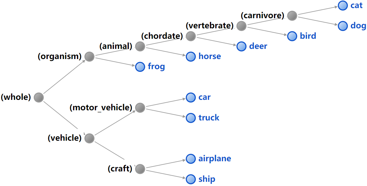
Figure 15: The generated class hierarchy when $r=0$.

Figure 16: The generated class hierarchy when $r=0.1$.

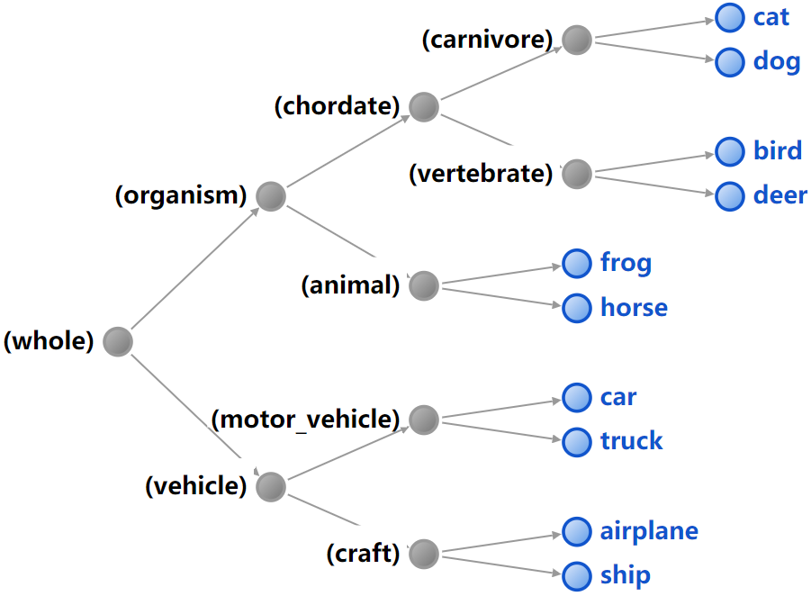
Figure 17: The generated class hierarchy when $r=0.2$.

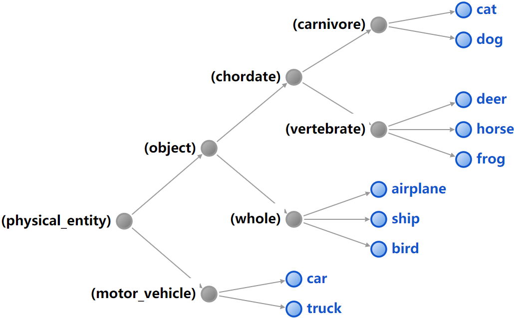
Figure 18: The generated class hierarchy when $r=0.3$.

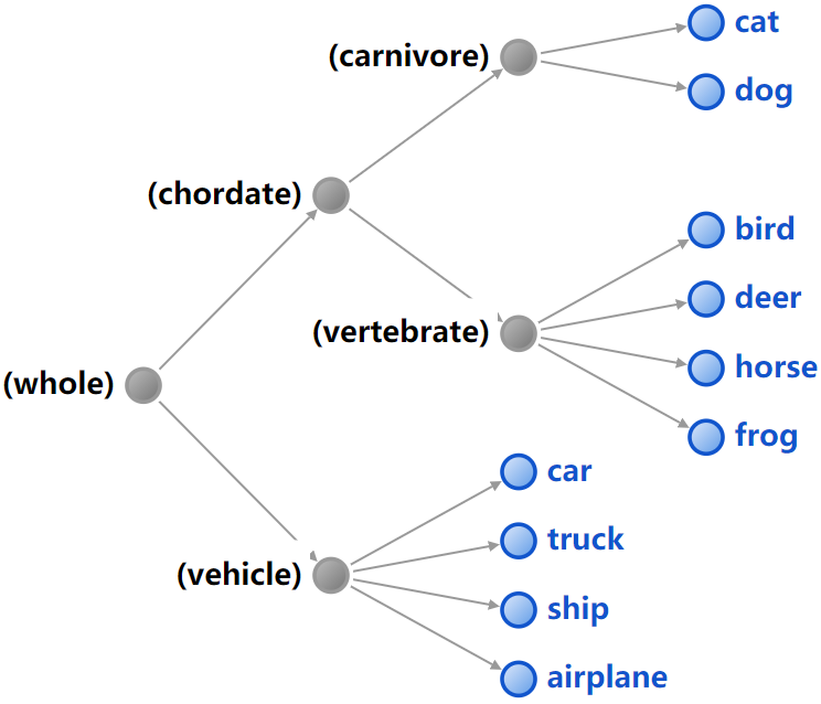
Figure 19: The generated class hierarchy when $r=0.8$.

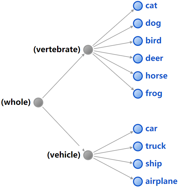
Figure 20: The generated class hierarchy when $r\geq 1.0$.

References

- Brust and Denzler (2019) Brust, C.-A.; and Denzler, J. 2019. Integrating domain knowledge: using hierarchies to improve deep classifiers. In Asian Conference on Pattern Recognition, 3–16. Springer.
- Cavalin and Oliveira (2018) Cavalin, P.; and Oliveira, L. 2018. Confusion matrix-based building of hierarchical classification. In Iberoamerican Congress on Pattern Recognition, 271–278. Springer.
- Corpet (1988) Corpet, F. 1988. Multiple sequence alignment with hierarchical clustering. Nucleic acids research, 16(22): 10881–10890.
- Fawcett (2006) Fawcett, T. 2006. An Introduction to ROC Analysis. Pattern Recognition Letters, 27(8): 861–874.
- Frosst and Hinton (2017) Frosst, N.; and Hinton, G. 2017. Distilling a neural network into a soft decision tree. arXiv preprint arXiv:1711.09784.
- Gao and Koller (2011) Gao, T.; and Koller, D. 2011. Discriminative learning of relaxed hierarchy for large-scale visual recognition. In 2011 international conference on computer vision, 2072–2079. IEEE.
- Govender and Sivakumar (2020) Govender, P.; and Sivakumar, V. 2020. Application of k-means and hierarchical clustering techniques for analysis of air pollution: A review (1980–2019). Atmospheric Pollution Research, 11(1): 40–56.
- He et al. (2016) He, K.; Zhang, X.; Ren, S.; and Sun, J. 2016. Deep residual learning for image recognition. In Proceedings of the IEEE conference on computer vision and pattern recognition, 770–778.
- Krizhevsky, Hinton et al. (2009) Krizhevsky, A.; Hinton, G.; et al. 2009. Learning multiple layers of features from tiny images.
- Li et al. (2019) Li, A.; Luo, T.; Lu, Z.; Xiang, T.; and Wang, L. 2019. Large-scale few-shot learning: Knowledge transfer with class hierarchy. In Proceedings of the IEEE/CVF Conference on Computer Vision and Pattern Recognition, 7212–7220.
- Marszalek and Schmid (2007) Marszalek, M.; and Schmid, C. 2007. Semantic hierarchies for visual object recognition. In 2007 IEEE Conference on Computer Vision and Pattern Recognition, 1–7. IEEE.
- Pan and Shen (2020) Pan, X.; and Shen, H.-B. 2020. Scoring disease-microRNA associations by integrating disease hierarchy into graph convolutional networks. Pattern Recognition, 105: 107385.
- Quinlan (1983) Quinlan, J. R. 1983. Learning Efficient Classification Procedures and Their Application to Chess End Games. In Michalski, R. S.; Carbonell, J. G.; and Mitchell, T. M., eds., Machine Learning: An Artificial Intelligence Approach, 463–482. Berlin, Heidelberg: Springer Berlin Heidelberg.
- Rama and Çöltekin (2017) Rama, T.; and Çöltekin, Ç. 2017. Fewer features perform well at native language identification task. In Proceedings of the 12th Workshop on Innovative Use of NLP for Building Educational Applications, 255–260.
- Senac et al. (2017) Senac, C.; Pellegrini, T.; Mouret, F.; and Pinquier, J. 2017. Music feature maps with convolutional neural networks for music genre classification. In Proceedings of the 15th International Workshop on Content-Based Multimedia Indexing, 1–5.
- Simoes, Almeida, and Byers (2014) Simoes, A.; Almeida, J. J.; and Byers, S. D. 2014. Language identification: a neural network approach. In 3rd Symposium on Languages, Applications and Technologies. Schloss Dagstuhl-Leibniz-Zentrum fuer Informatik.
- Wan et al. (2021) Wan, A.; Dunlap, L.; Ho, D.; Yin, J.; Lee, S.; Jin, H.; Petryk, S.; Bargal, S. A.; and Gonzalez, J. E. 2021. NBDT: Neural-backed decision trees. In ICLR’21. ArXiv preprint arXiv:2004.00221.
- Ward Jr (1963) Ward Jr, J. H. 1963. Hierarchical grouping to optimize an objective function. Journal of the American statistical association, 58(301): 236–244.
- Wikipedia contributors (2021a) Wikipedia contributors. 2021a. Germanic languages — Wikipedia, The Free Encyclopedia. [Online; accessed 5-September-2021].
- Wikipedia contributors (2021b) Wikipedia contributors. 2021b. Jazz — Wikipedia, The Free Encyclopedia. [Online; accessed 6-September-2021].
- Xiong (2012) Xiong, Y. 2012. Building text hierarchical structure by using confusion matrix. In 2012 5th International Conference on BioMedical Engineering and Informatics, 1250–1254. IEEE.
- Zagoruyko and Komodakis (2016) Zagoruyko, S.; and Komodakis, N. 2016. Wide residual networks. arXiv preprint arXiv:1605.07146.
- Zhao, Karypis, and Fayyad (2005) Zhao, Y.; Karypis, G.; and Fayyad, U. 2005. Hierarchical clustering algorithms for document datasets. Data mining and knowledge discovery, 10(2): 141–168.