Temperature–dependence of the subdivision potential in nanothermodynamics

Abstract

Nanothermodynamics is the thermodynamics of small systems, which are significantly affected by their surrounding environments. In nanothermodynamics, Hill introduced the concept of subdivision potential, which charaterizes the non-extensiveness. In this work, we establish the quantum thermodynamic integration of the subdivision potential, which is identified to be proportional to the difference between the thermal and von Neumann entropies, focusing on its temperature–dependence. As a result, it serves as a versatile tool to help analyze the origin of non-extensiveness in nanosystems.

Introduction –

Systems are inevitably interacting with the environments in which they are embedded. A system is referred to be small, if it is significantly affected by the surrounding environments. For small systems, classical thermodynamics, remarked by Einstein as “the only physical theory which I am convinced will never be overthrown within the framework of applicability of its basic concepts” Ein79 , is not directly suitable since the non-extensiveness. In 1962, Hill proposed the nanothermodynamics Hil623182 ; Hil63 , which adds an subdivision potential term to the traditional Gibbs equation, reading

$$E=U+\varepsilon\equiv TS-pV+\mu N+\varepsilon.$$ (1)

Equation (1) is known as the Gibbs–Hill equation, where $\varepsilon$ is nothing but the subdivision potential. This approach intrigues widespread interests among various fields of modern sciences Hil01111 ; Hil01273 ; Cha1552 ; Qia12201 ; Bed20 .

For a system at finite temperate $T$, with constant volume $V$ and particle number $N$, the Helmholtz free energy $F=E-TS$ is related to partition function $Z$ as

$$F=-\beta^{-1}\ln Z.$$ (2)

Throughout this paper, we set $\beta=1/(k_{B}T)$, with $k_{B}$ and $T$ being the Boltzmann constant and temperature, respectively. For simplicity, we always set $k_{B}=1$ below.

For large systems, which is extensive due to the thermodynamic limit, $Z$ characterizes the canonical ensemble, i.e.,

$$Z={\rm tr}_{\mbox{\tiny S}}\big{(}e^{-\beta H_{\mbox{\tiny S}}}\big{)}\longrightarrow\ \ {{\rm cf.\,Eq.\,(\ref{Z})}}$$ (3)

with $H_{\mbox{\tiny S}}$ being the system Hamiltonian. This will lead to $\varepsilon=0$, resulting $E=U$ in Eq. (1). However, small systems are not distributed canonically due to their interactions with the environments, and in these cases Eq. (3) is violated and $\varepsilon\neq 0$. It is therefore necessary to modify the $Z$ in Eq. (3) and distinguish between $E$ and $U$.

Subdivision potential proportional to the difference between the thermal and von Neumann entropies –

Now turn to the discussion on the subdivision potential $\varepsilon$ of small systems. Since the system is small, as explained above, the environment and the system–environment interaction are necessarily involved. Consider a system–plus–environment composite Hamiltonian reading

$$H_{\mbox{\tiny T}}=H_{\mbox{\tiny S}}+H_{\mbox{\tiny SB}}+h_{\mbox{\tiny B}},$$ (4)

where $H_{\mbox{\tiny S}}$, $H_{\mbox{\tiny SB}}$ and $h_{\mbox{\tiny B}}$ are the system, the system–environment interaction and the environment Hamiltonians, respectively. To identify the subdivsion potential $\varepsilon$, one may follow Landsberg and introduce the temperature–dependent Hamiltonian $H_{\mbox{\tiny S}}(\beta)$ as Elc57161 ; Mig202471

$$H_{\mbox{\tiny S}}(\beta)\equiv-\beta^{-1}\big{[}\ln{\rm tr}_{\mbox{\tiny B}}(e^{-\beta H_{\mbox{\tiny T}}})-\ln Z_{\mbox{\tiny B}}\big{]},$$ (5)

with $Z_{\mbox{\tiny B}}={\rm tr}_{\mbox{\tiny B}}(e^{-\beta h_{\mbox{\tiny B}}})$. In this formalism, the system density operator is

$$\rho_{\mbox{\tiny S}}(\beta)=\frac{e^{-\beta H_{\mbox{\tiny S}}(\beta)}}{Z}=\frac{{\rm tr}_{\mbox{\tiny B}}\big{(}e^{-\beta H_{\mbox{\tiny T}}}\big{)}}{Z_{\mbox{\tiny T}}},$$ (6)

where the partition functions are [cf. Eq. (3)]

$$Z={\rm tr}_{\mbox{\tiny S}}\big{[}e^{-\beta H_{\mbox{\tiny S}}(\beta)}\big{]}=\frac{Z_{\mbox{\tiny T}}}{Z_{\mbox{\tiny B}}}\ \ \text{and}\ \ Z_{\mbox{\tiny T}}={\rm Tr}\big{(}e^{-\beta H_{\mbox{\tiny T}}}\big{)}.$$ (7)

In this paper, ${\rm Tr}$, ${\rm tr}_{\mbox{\tiny S}}$ and ${\rm tr}_{\mbox{\tiny B}}$ represent the total trace, the system and the environmental subspace partial trace, respectively. Since the bath is less affected by the system, we identify the $E$ as difference between the energy of total system $E_{\mbox{\tiny T}}$ and that of bath $E_{\mbox{\tiny B}}$, leading to the equality

$$E=E_{\mbox{\tiny T}}-E_{\mbox{\tiny B}}=-\frac{\partial\ln(Z_{\mbox{\tiny T}}/Z_{\mbox{\tiny B}})}{\partial\beta}=-\frac{\partial\ln Z}{\partial\beta},$$ (8)

where $E_{\mbox{\tiny T}}=-\partial\ln Z_{\mbox{\tiny T}}/\partial\beta$ and $E_{\mbox{\tiny B}}=-\partial\ln Z_{\mbox{\tiny B}}/\partial\beta$. On the other hand, the thermodynamic internal energy of system $U$ is considered as the average of $H_{\mbox{\tiny S}}(\beta)$, namely

$$U=\langle H_{\mbox{\tiny S}}(\beta)\rangle\equiv Z^{-1}{\rm tr}_{\mbox{\tiny S}}\big{[}H_{\mbox{\tiny S}}(\beta)e^{-\beta H_{\mbox{\tiny S}}(\beta)}\big{]}.$$ (9)

Therefore, we can identify the subdivision potential as [cf.  Eqs. (1), (8) and (9)]

$$\varepsilon=-\frac{\partial\ln Z}{\partial\beta}-\langle H_{\mbox{\tiny S}}(\beta)\rangle=\beta\Big{\langle}\frac{\partial H_{\mbox{\tiny S}}(\beta)}{\partial\beta}\Big{\rangle}.$$ (10)

To exhibit the temperature dependence of $\varepsilon$, we first rewrite $\langle H_{\mbox{\tiny S}}(\beta)\rangle$ as

$$\langle H_{\mbox{\tiny S}}(\beta)\rangle=-\beta^{-1}\big{\{}{\rm tr}_{\mbox{\tiny S}}[\rho_{\mbox{\tiny S}}(\beta)\ln\rho_{\mbox{\tiny S}}(\beta)]+\ln Z\big{\}},$$ (11)

and it together with Eq. (10) shows that

$$\varepsilon=\beta^{-1}[S_{\rm therm}(\beta)-S_{\rm vN}(\beta)]$$ (12)

with the thermal entropy:

$$S_{\rm therm}(\beta)=-\frac{\partial F}{\partial T}=\beta^{2}\frac{\partial F}{\partial\beta},$$ (13)

and the von Neumann entropy:

$$S_{\rm vN}(\beta)=-{\rm tr}_{\mbox{\tiny S}}[\rho_{\mbox{\tiny S}}(\beta)\ln\rho_{\mbox{\tiny S}}(\beta)].$$ (14)

Here, the free–energy $F$ is defined in Eq. (2) with partition function $Z$ in Eq. (7). Apparently, Eq. (12) tells us that the subdivision potential $\varepsilon$ is proportional to the difference between the thermal entropy $S_{\rm therm}(\beta)$ and the von Neumann entropy $S_{\rm vN}(\beta)$, as defined in Eqs. (13) and (14), respectively. It is reasonable to render the difference arises from that the thermodynamic limit is not satisfied for small systems.

Thermodynamic integration –

Now, we apply the thermodynamic integration for the free energy $F$, as done in our previous works Gon20154111 ; Gon20214115 .

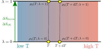
Figure 1: An illustrative depiction of the thermodynamic integration, Eq. (Thermodynamic integration –). The theoretical details can be found in Ref. [Gon20214115, ]

Consider a $\lambda$–augmented form of Eq. (4), reading

$$H_{\mbox{\tiny T}}(\lambda)=H_{\mbox{\tiny S}}+\lambda H_{\mbox{\tiny SB}}+h_{\mbox{\tiny B}},$$ (15)

with $\lambda\in[0,1]$ characterizing the hybridization. Consider the a hybridization process with respect to $\lambda$, at a constant temperature $T$, as depicted in Fig. 1. The free energy change can be written in the integration form Gon20154111 ; Gon20214115

$$\Delta F(T) \equiv F(T;\lambda=1)-F(T;\lambda=0),$$

$$=\int_{0}^{1}\!\frac{{\rm d}\lambda}{\lambda}\,{\rm Tr}[(\lambda H_{\mbox{\tiny SB}})\rho_{\mbox{\tiny T}}(T;\lambda)],$$ (16)

with $\rho_{\mbox{\tiny T}}(T;\lambda)=e^{-\beta H_{\mbox{\tiny T}}(\lambda)}/Z_{\mbox{\tiny T}}(\beta;\lambda)$.

We can obtain $\Delta F(T)$ in Eq. (Thermodynamic integration –) according to the Kirkwood thermodynamics integration as

$$\Delta F(T) =\int^{1}_{0}\!\frac{{\rm d}\Delta F(T)}{{\rm d}\lambda}{\rm d}\lambda$$

$$=-\frac{1}{\beta}\int^{1}_{0}\!\frac{{\rm d}\lambda}{Z_{\mbox{\tiny T}}(\lambda)}{\rm Tr}\Big{[}\frac{{\rm d}}{{\rm d}\lambda}e^{-\beta(H_{\mbox{\tiny S}}+h_{\mbox{\tiny B}}+\lambda H_{\mbox{\tiny SB}})}\Big{]}.$$ (17)

It leads to $\Delta F(T)$ in Eq. (Thermodynamic integration –), due to the following relation:

$$-\frac{1}{\beta}{\rm Tr}\Big{[}\frac{{\rm d}}{{\rm d}\lambda}e^{-\beta(H_{\mbox{\tiny S}}+h_{\mbox{\tiny B}}+\lambda H_{\mbox{\tiny SB}})}\Big{]}={\rm Tr}\Big{[}H_{\mbox{\tiny SB}}e^{-\beta(H_{\mbox{\tiny S}}+h_{\mbox{\tiny B}}+\lambda H_{\mbox{\tiny SB}})}\Big{]}.$$

This relation is a special case of the general relation reading

$${\rm Tr}\Big{[}\frac{{\rm d}}{{\rm d}\lambda}e^{O(\lambda)}\Big{]}={\rm Tr}\Big{[}\frac{{\rm d}O(\lambda)}{{\rm d}\lambda}e^{O(\lambda)}\Big{]},$$

which can be proved via the operator identity

$$\frac{{\rm d}}{{\rm d}\lambda}e^{O(\lambda)}=\int_{0}^{1}\!{{\rm d}s}\,e^{(1-s)O(\lambda)}\frac{{\rm d}O(\lambda)}{{\rm d}\lambda}e^{sO(\lambda)}$$

and the trace cyclic invariance.

As a result, Eqs. (10) and (Thermodynamic integration –) give rise to

$$\varepsilon(T) =T\left[-\frac{\partial F(T;\lambda=1)}{\partial T}-S_{\rm vN}(\beta)\right]$$

$$=T\!\left[-\frac{\partial\Delta F(T)}{\partial T}-\frac{\partial F(T;\lambda=0)}{\partial T}-S_{\rm vN}(\beta)\right]$$

$$=T[\Delta S_{\rm therm}(T)-\Delta S_{\rm vN}(T)].$$ (18)

In Eq. (Thermodynamic integration –), we have defined $\Delta S_{\rm therm/vN}(T)\equiv S_{\rm therm/vN}(T;\lambda=1)-S_{\rm therm/vN}(T;\lambda=0)$ and used the equality $S_{\rm vN}(T;\lambda=0)=S_{\rm therm}(T;\lambda=0)$ due to the canonicity in the absence of system–bath interactions. Numerically, all these quantities can be computed via the dissipaton-equation-of-motion method ($\lambda$-dynamics formalism or imaginary–time formalism) Yan14054105 ; Gon20154111 ; Gon20214115 , which is a second quantization generalization of the well–known hierarachical equations of motion, serving as a rigid approach to the dynamics of a specific system coupled to the Gaussian environments Tan89101 ; Tan906676 ; Yan04216 ; Xu05041103 .

Example –

As an example, we consider a spin–boson model

$$H_{\mbox{\tiny T}}(\lambda)=(E\hat{\sigma}_{z}+V\hat{\sigma}_{x})+\lambda\hat{\sigma}_{z}\hat{F}+h_{\mbox{\tiny B}},$$ (19)

with $h_{\mbox{\tiny B}}$ being harmonic and the hybrid bath modes $\hat{F}$ being linear, i.e., $h_{\mbox{\tiny B}}=\frac{1}{2}\sum_{j}\omega_{j}(\hat{p}_{j}^{2}+\hat{x}_{j}^{2})\ \ {\rm and}\ \ \hat{F}=\sum_{j}c_{j}\hat{x}_{j}.$ The computational results are shown in Fig. 2, with parameters given in the caption.

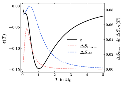
Figure 2: Tempature–dependenece of the subvivision potential. Parameters are taken in accordance to that in Ref. [Gon20154111, ]. The bath spectral density $J(\omega)=(\pi/2)\sum_{j}c_{j}^{2}\delta(\omega-\omega_{j})$ takes the Drude form as $J(\omega)=\eta\gamma\omega/(\omega^{2}+\gamma^{2})$ with parameters: $\gamma=4V$ and $\eta=0.5V$. The spin energy difference is $E=0.5V$, and the temperature is scaled by the system charateristic frequency $\Omega_{\mbox{\tiny S}}\equiv 2\sqrt{E^{2}+V^{2}}$.

In Fig. 2, we show the temperature dependence of $\varepsilon(T)$, as well as $\Delta S_{\rm therm}(T)$ and $\Delta S_{\rm vN}(T)$. The temperature is scaled by the system charateristic frequency $\Omega_{\mbox{\tiny S}}\equiv 2\sqrt{E^{2}+V^{2}}$ . It is observed that the subdivision potential exhibits a turnover near the characteristic frequency, and this is conjectured as a universal feature.

Summary –

In summary, we first identify the subdivision potential $\varepsilon$ to be proportional to the difference between the thermal and von Neumann entropies, followed by the establishment of its quantum thermodynamic integration. We explicitly show its temperature–dependence by taking the spin–boson model as an example, and one characteristic turnover point of subdivision potential is observed. Besides, the method developed in this work serves as a versatile tool to help analyze the origin of non-extensiveness in nanosystems.

Support from the Ministry of Science and Technology of China, Grant No. 2017YFA0204904, and the National Natural Science Foundation of China, Nos. 21633006, 22103073 and 22173088 is gratefully acknowledged. This research is partially motivated by the 1st “Question and Conjecture” activity supported by the Top Talent Training Program 2.0 for undergraduates.

References

- (1) A. Einstein, in Autobiographical Notes, edited by P. A. Schilpp, Open Court Publishing, La Salle, 1979.
- (2) T. L. Hill, J. Chem. Phys. 36, 3182 (1962).
- (3) T. L. Hill, Thermodynamics of Small Systems. Part 1 and 2, Benjamin, New York, 1963.
- (4) T. L. Hill, Nano Lett. 1, 111 (2001).
- (5) T. L. Hill, Nano Lett. 1, 273 (2001).
- (6) R. V. Chamberlin, Entropy 17(1), 52 (2015).
- (7) H. Qian, J. Biol. Phys. 38-2, 201 (2012).
- (8) D. Bedeaux, S. Kjelstrup, and S. K. Schnell, Nanothermodynamics: General Theory, PoreLab, Trondheim, 2020.
- (9) E. W. Elcock and P. T. Landsberg, Proc. Phys. Soc. Lond. Sect. B 70, 161 (1957).
- (10) R. de Miguel and J. M. Rubí, Nanomaterials 10-12, 2471 (2020).
- (11) H. Gong, Y. Wang, H. D. Zhang, Q. Qiao, R. X. Xu, X. Zheng, and Y. J. Yan, J. Chem. Phys. 153, 154111 (2020).
- (12) H. Gong, Y. Wang, H. D. Zhang, R. X. Xu, X. Zheng, and Y. J. Yan, J. Chem. Phys. 153, 214115 (2020).
- (13) Y. J. Yan, J. Chem. Phys. 140, 054105 (2014).
- (14) Y. Tanimura and R. Kubo, J. Phys. Soc. Jpn. 58, 101 (1989).
- (15) Y. Tanimura, Phys. Rev. A 41, 6676 (1990).
- (16) Y. A. Yan, F. Yang, Y. Liu, and J. S. Shao, Chem. Phys. Lett. 395, 216 (2004).
- (17) R. X. Xu, P. Cui, X. Q. Li, Y. Mo, and Y. J. Yan, J. Chem. Phys. 122, 041103 (2005).