Homes’ law in holographic superconductor with linear-$T$ resistivity

Abstract

Homes’ law, $\rho_{s}=C\,\sigma_{DC}\,T_{c}$, is a universal relation of superconductors between the superfluid density $\rho_{s}$ at zero temperature, the critical temperature $T_{c}$ and the electric DC conductivity $\sigma_{DC}$ at $T_{c}$. Experimentally, Homes’ law is observed in high $T_{c}$ superconductors with linear-$T$ resistivity in the normal phase, giving a material independent universal constant $C$. By using holographic models related to the Gubser-Rocha model, we investigate how Homes’ law can be realized together with linear-$T$ resistivity in the presence of momentum relaxation. We find that strong momentum relaxation plays an important role to exhibit Homes’ law with linear-$T$ resistivity.

1 Introduction

Holographic methods (gauge/gravity duality) have been providing novel and effective ways to study universal properties of strongly correlated systems. The representative examples would be the holographic lower bound of the ratio of shear viscosity to entropy density, linear-$T$ resistivity and Hall angle of strange metals Hartnoll:2016apf ; Zaanen:2015oix ; Ammon:2015wua ; Baggioli:2019rrs ; Hartnoll:2009sz ; Herzog:2009xv .

In this paper, using holography, we study another universal property of strongly coupled systems, which is observed in high $T_{c}$ superconductors and some conventional superconductors: Homes’ law Homes:2005aa ; Homes:2004wv . Homes’ law is an empirical relation between the superfluid density at $T=0$ ($\rho_{s}(T=0)$), the phase transition temperature ($T_{c}$), and the electric DC conductivity in the normal phase close to $T_{c}$ ($\sigma_{DC}(T_{c})$):

$$\rho_{s}(T=0)\,=\,C\,\sigma_{DC}(T_{c})\,T_{c}\,,$$ (1)

where $C$ is a material independent universal constant. For instance, $C\sim 4.4$ for ab-plane high $T_{c}$ superconductors and clean BCS superconductors or $C\sim 8.1$ for c-axis high $T_{c}$ superconductors and BCS superconductors in the dirty limit.

In order to study Homes’ law in holography, first one may need to construct the holographic superconductor model. Using the complex scalar field, the holographic superconductor model was originally proposed by Hartnoll, Herzog, and Horowitz Hartnoll:2008vx ; Hartnoll:2008kx (the HHH model). Thereafter, there has been extensive development and extension of the HHH model in Hartnoll:2009sz ; Herzog:2009xv ; Horowitz:2010gk ; Cai:2015cya . For the recent development of holographic superconductors, see also Kim:2013oba ; Gouteraux:2019kuy ; Gouteraux:2020asq ; Arean:2021brz ; Donos:2021pkk ; Ammon:2021slb and references therein.

Since the HHH model is a translational invariant theory, $\sigma_{DC}$ is infinite so $C$ in (1) is not well defined. Thus, in order to investigate Homes’ law, one may need to break the translational invariance to render $\sigma_{DC}$ finite. In holography, there are several methods to incorporate momentum relaxation and yield a finite $\sigma_{DC}$. For instance, the bulk fields in gravity with the inhomogeneous boundary conditions Horowitz:2012ky , massive gravity models Vegh:2013sk , Q-lattice models Donos:2013eha , the linear axion model Andrade:2013gsa , and the helical lattice model with a Bianchi VII₀ symmetry Donos:2012js . Using these models, holographic superconductors in the presence of the momentum relaxation have been investigated in Erdmenger:2015qqa ; Horowitz:2013jaa ; Zeng:2014uoa ; Ling:2014laa ; Andrade:2014xca ; Kim:2015dna ; Baggioli:2015zoa ; Baggioli:2015dwa ; Kim:2016hzi ; Kim:2016jjk ; Ling:2016lis ; Jeong:2018tua .

In the aforementioned holographic superconductor models with momentum relaxation, Homes’ law has been studied only in several models Erdmenger:2015qqa ; Kim:2016jjk ; Kim:2016hzi . For those models, there are parameters for the strength of momentum relaxation, which may specify material properties. Thus, in the holographic setup, Homes’ law means that $C$ in (1) is constant independent of momentum relaxation parameters. In Erdmenger:2015qqa , using the helical lattice model, Homes’ law was studied with the amplitude and the pitch of the helix as momentum relaxation parameters. In Kim:2016hzi , the linear axion model was studied for Homes’ law with the the proportionality constant to spatial coordinate, $k$ in (8), for the strength of momentum relaxation. In Kim:2016jjk , the Q-lattice model was used to study Homes’ law with the lattice amplitude/wavenumber for momentum relaxation parameter.

In all holographic studies so far, Homes’ law has not been well realized in that, in Erdmenger:2015qqa ; Kim:2016jjk , Homes’ law is satisfied only for some restricted parameter regime in which underlying physics has not been clearly understood yet or Homes’ law is not simply satisfied in Kim:2016hzi . Therefore, the fundamental understanding and the physical mechanism of Homes’ law is still lacking and it would be important to study Homes’ law with other holographic models.

In this paper, we study Homes’ law in the holographic superconductor model based on the Gubser-Rocha model Gubser:2009qt with the axion field to have momentum relaxation Davison:2013txa ; Zhou:2015qui ; Kim:2017dgz ; Jeong:2018tua ; Liu:2021qmt . Our main motivation to choose this model is that it exhibits linear-$T$ resistivity in its normal phase Davison:2013txa ; Zhou:2015qui ; Jeong:2018tua . In particular, in Jeong:2018tua , it was shown that the linear-$T$ resistivity is robust above $T_{c}$ in the strong momentum relaxation limit, which is similar to the experimental result for normal phases (strange metal phases) of high $T_{c}$ superconductors. We will examine if Homes’ law can appear also in the strong momentum relaxation limit and also study its relation with the linear-$T$ resistivity.

The property of linear-$T$ resistivity is important for two reasons. First, it is another universal property in the normal phase of high $T_{c}$ superconductors, so it is in fact a necessary property even before discussing Homes’ law. Second, it has been proposed that the Homes’ law can be explained by considering the Planckian dissipation Zaanen:2004aa , which is related with the linear-$T$ resistivity. Therefore, the linear-$T$ resistivity can be a key to understand the physics of Homes’ law. Because there has been no holographic model studying Homes’ law together with linear-$T$ resistivity our study is a necessary and important step to investigate Homes’ law. Moreover, the Gubser-Rocha model with the axion field allows an analytic solution so that more tractable analysis is available for the normal phase. Note that most holographic studies in Erdmenger:2015qqa ; Kim:2016jjk ; Kim:2016hzi do not allow analytic solution for normal phase so one needs to resort to numerical methods.

As one of the ingredient of our holographic superconductor model, inspired by Lucas:2014zea ; Cremonini:2016bqw , we introduce the non-trivial coupling, $B(\phi)$, between the dilaton field $\phi$ and the complex scalar field $\Phi$ for condenstate, and study the role of the coupling in Homes’ law. In Lucas:2014zea ; Cremonini:2016bqw , using the scaling property from $B(\phi)$, the superconducting instabilities have been investigated in which the translational invariance was not broken. Thus, our work might be considered as its generalization with momentum relaxation. Note that $B(\phi)$ was taken to be a mass term of $\Phi$, $B(\phi)=M^{2}$, in the previous literature for Homes’ law Erdmenger:2015qqa ; Kim:2016jjk ; Kim:2016hzi . We find that Homes’ law may not be realized with this trivial mass term.

This paper is organized as follows. In section 2, we introduce the holographic superconductor models based on the Gubser-Rocha model with the axion fields. In normal phase, we review how to obtain the linear-$T$ resistivity analytically. For superconductor phase, we introduce the coupling term $B(\phi)$ and review its properties. We also study superconducting instability with $T_{c}$. In section 3, we numerically compute the optical conductivity and study the superfluid density. Using the linear-$T$ resistivity in section 2 with the superfluid density in section 3, we study Homes’ law. We also discuss the role of the coupling $B(\phi)$ for Homes’ law. In section 4, we conclude.

2 Superconductor based on the Gubser-Rocha model

2.1 Model

We study a holographic superconductor model based on Einstein-Maxwell-Dilaton-Axion theory:

$$\begin{split}S&=S_{1}+S_{2}+S_{3}=\int\mathrm{d}^{4}x\sqrt{-g}\left(\mathcal{L}_{1}+\mathcal{L}_{2}+\mathcal{L}_{3}\right)\,,\\ \mathcal{L}_{1}&=R\,-\,\frac{1}{2}(\partial{\phi})^{2}\,-\,\frac{1}{4}e^{\frac{\phi}{\sqrt{3}}}\,F^{2}\,+\,6\cosh\left(\frac{\phi}{\sqrt{3}}\right)\,,\\ \mathcal{L}_{2}&=-\frac{1}{2}\sum_{I=1}^{2}(\partial\psi_{I})^{2}\,,\qquad\mathcal{L}_{3}=-|D\Phi|^{2}\,-B(\phi)|\Phi|^{2}\,,\end{split}$$ (2)

where we set units such that the AdS radius $L=1$, and the gravitational constant $16\pi G=1$. The action (2) consists of three actions. The first action $S_{1}$ is the Einstein-Maxwell-Dilaton theory, which is called ‘Gubser-Rocha model’ Gubser:2009qt composed of three fields: metric $g_{\mu\nu}$, a $U(1)$ gauge field $A_{\mu}$ with the field strength $F=\mathrm{d}A$, and the scalar field $\phi$ so called ‘dilaton’. The metric and gauge field are for a quantum field theory at finite temperature and density, while the dilaton field was originally introduced to make the vanishing entropy density ($s$) at zero temperature ($T$) as $s\sim T$ Gubser:2009qt ; Davison:2013txa . The second action $S_{2}$ is added for the momentum relaxation: the ‘axion’ field $\psi$ breaks the translational invariance so that the resistivity becomes finite Andrade:2013gsa ; Davison:2013txa ; Zhou:2015qui ; Kim:2017dgz ; Jeong:2018tua . The third action $S_{3}$ is for the superconducting phase Hartnoll:2008vx , which is composed of a complex scalar field $\Phi$, the coupling $B(\phi)$, and the covariant derivative defined by $D_{\mu}:=\nabla_{\mu}-iqA_{\mu}$.

The action (2) yields the equations of motion of matter fields

$$\nabla_{\mu}(e^{\frac{\phi}{\sqrt{3}}}F^{\mu\nu})-iq\Phi^{*}(\partial^{\nu}-iqA^{\nu})\Phi+iq\Phi(\partial^{\nu}+iqA^{\nu})\Phi^{*}=0\,,$$ (3)

$$\nabla^{2}\phi-\frac{1}{4\sqrt{3}}e^{\frac{\phi}{\sqrt{3}}}\,F^{2}+2\sqrt{3}\,\sinh\left(\frac{\phi}{\sqrt{3}}\right)-B^{\prime}(\phi)|\Phi|^{2}=0\,,$$ (4)

$$\nabla^{2}\psi_{I}=0\,,$$ (5)

$$D^{2}\Phi-B(\phi)\Phi=0\,,$$ (6)

and the Einstein’s equation

$$\begin{split}&R_{\mu\nu}-\frac{1}{2}g_{\mu\nu}\left[R-\frac{1}{4}e^{\frac{\phi}{\sqrt{3}}}F^{2}-\frac{1}{2}(\partial{\phi})^{2}+6\cosh\left(\frac{\phi}{\sqrt{3}}\right)-\frac{1}{2}\sum_{I=1}^{2}(\partial\psi_{I})^{2}-|D\Phi|^{2}-B(\phi)|\Phi|^{2}\right]\\ &\qquad=\frac{1}{2}e^{\frac{\phi}{\sqrt{3}}}F_{\mu\delta}F_{\nu}{{}^{\delta}}+\frac{1}{2}\partial_{\mu}\phi\partial_{\nu}\phi+\frac{1}{2}\sum_{I=1}^{2}(\partial_{\mu}\psi_{I}\partial_{\nu}\psi_{I})+\frac{1}{2}\left(D_{\mu}\Phi D_{\nu}^{*}\Phi^{*}+D_{\nu}\Phi D_{\mu}^{*}\Phi^{*}\right)\,.\end{split}$$ (7)

2.2 Linear-$T$ resistivity in strange metal phase: a quick review

Let us first review the normal phase ($\Phi=0$), $S=S_{1}+S_{2}$, i.e., the Gubser-Rocha model with momentum relaxation. The purpose of this review is not only to organize this paper in a self-contained manner, but also collect useful results, linear-$T$ resistivity, to study our main objective, Homes’ law, in section 3. We refer to Jeong:2018tua for more detailed explanation of the normal phase.

In normal phase ($\Phi=0$), the analytic solution is available Cremonini:2016bqw ; Zhou:2015qui ; Kim:2017dgz ; Jeong:2018tua :

$$\begin{split}&\mathrm{d}s^{2}=-f(r)\mathrm{d}t^{2}+\frac{1}{f(r)}\mathrm{d}r^{2}+h(r)(\mathrm{d}x^{2}+\mathrm{d}y^{2}),\\ &f=r^{1/2}(r+Q)^{3/2}\left(1-\frac{k^{2}}{2(r+Q)^{2}}-\frac{(r_{h}+Q)^{3}}{(r+Q)^{3}}\left(1-\frac{k^{2}}{2(r_{h}+Q)^{2}}\right)\right),\\ &h=r^{1/2}(r+Q)^{3/2},\\ &A_{t}=\sqrt{3Q(r_{h}+Q)\left(1-\frac{k^{2}}{2(r_{h}+Q)^{2}}\right)}\left(1-\frac{r_{h}+Q}{r+Q}\right),\quad\phi=\frac{\sqrt{3}}{2}\ln(1+Q/r)\,,\\ &\psi_{1}=k\,x\,,\quad\psi_{2}=k\,y\,,\end{split}$$ (8)

where $r_{h}$ denotes the horizon radius, $k$ controls a strength of the momentum relaxation, and $Q$ is a parameter which can be expressed with physical parameters: temperature ($T$), chemical potential ($\mu$) or momentum relaxation parameter ($k$). The temperature and chemical potential reads

$$T=\frac{f^{\prime}(r)}{4\pi}\Bigr{|}_{r_{h}}={r_{h}}\frac{6(1+{\tilde{Q}})^{2}-\mbox{${\tilde{k}}$}^{2}}{8\pi(1+{\tilde{Q}})^{3/2}}=r_{h}\mbox{$\tilde{T}$}\,,$$ (9)

$$\mu=A_{t}(\infty)=r_{h}\sqrt{3{\tilde{Q}}(1+{\tilde{Q}})\left(1-\frac{\mbox{${\tilde{k}}$}^{2}}{2(1+{\tilde{Q}})^{2}}\right)}=r_{h}{\tilde{\mu}}\,,$$ (10)

where

$$\tilde{Q}:=\frac{Q}{r_{h}}\,,\qquad\tilde{k}:=\frac{k}{r_{h}}\,,\qquad\tilde{T}:=\frac{T}{r_{h}}\,,\qquad\tilde{\mu}:=\frac{\mu}{r_{h}}\,.$$ (11)

Now one can obtain the dimensionless physical quantities at finite density, $T/\mu$ and $k/\mu$, as

$$\mbox{${\bar{T}}$}:=\frac{T}{\mu}=\frac{\mbox{$\tilde{T}$}}{{\tilde{\mu}}}=\frac{6(1+{\tilde{Q}})^{2}-\tilde{k}^{2}}{4\sqrt{6}\pi\sqrt{{\tilde{Q}}(1+{\tilde{Q}})^{2}(2(1+{\tilde{Q}})^{2}-\tilde{k}^{2})}}\,,$$ (12)

$$\mbox{${\bar{k}}$}:=\frac{k}{\mu}=\frac{\mbox{${\tilde{k}}$}}{{\tilde{\mu}}}=\sqrt{\frac{2(1+{\tilde{Q}})\tilde{k}^{2}}{3{\tilde{Q}}(2(1+{\tilde{Q}})^{2}-\tilde{k}^{2})}}\,,$$ (13)

where we used (9)-(11).

The linear-$T$ resistivity:

The electric DC conductivity at $\Phi=0$ can be obtained Donos:2014cya ; Blake:2013bqa ; Kim:2015wba ; Kim:2015sma as

$$\sigma_{DC}:=e^{\frac{\phi}{\sqrt{3}}}+\frac{A_{t}^{\prime 2}\,h(r)\,e^{\frac{2\phi}{\sqrt{3}}}}{k^{2}}\Bigr{|}_{r\rightarrow r_{h}}=\sqrt{1+{\tilde{Q}}}+\frac{\sqrt{1+{\tilde{Q}}}}{\mbox{${\bar{k}}$}^{2}}\,.$$ (14)

Using (12)-(13), one can express ${\tilde{Q}}$ as a function of ${\bar{T}}$ and ${\bar{k}}$ analytically, i.e. ${\tilde{Q}}(\mbox{${\bar{T}}$},\mbox{${\bar{k}}$})$, this implies that the electric DC conductivity (14) can also be expressed in terms of ${\bar{T}}$ and ${\bar{k}}$ as $\sigma_{DC}(\mbox{${\bar{T}}$},\mbox{${\bar{k}}$})$.

With the analytic expression of ${\tilde{Q}}(\mbox{${\bar{T}}$},\mbox{${\bar{k}}$})$, one can find that the Gubser-Rocha model can exhibit linear-$T$ resistivity, the resistivity ($\rho=1/\sigma_{DC}$) is linear in temperature, for two cases

$$\sigma_{DC}\,\sim\,\frac{\sqrt{3}\left(1+\mbox{${\bar{k}}$}^{2}\right)^{2}}{2\pi\mbox{${\bar{k}}$}^{2}\sqrt{4+6\mbox{${\bar{k}}$}^{2}}}\frac{1}{\mbox{${\bar{T}}$}}\,,\qquad\quad(\mbox{${\bar{T}}$}\ll 1\,\,\text{for given}\,\,\mbox{${\bar{k}}$})\,,$$ (15)

$$\sigma_{DC}\,\sim\,\frac{\mbox{${\bar{k}}$}}{2\sqrt{2}\pi\,\mbox{${\bar{T}}$}}\,,\qquad\qquad\qquad\,\,\ \ (\mbox{${\bar{k}}$}\gg 1\,\,\text{for given}\,\,\mbox{${\bar{T}}$})\,,$$ (16)

where ${\tilde{Q}}(\mbox{${\bar{T}}$},\mbox{${\bar{k}}$})$ has the asymptotic form as

$${\tilde{Q}}\sim\frac{3(1+\mbox{${\bar{k}}$}^{2})^{2}}{8\pi^{2}(2+3\mbox{${\bar{k}}$}^{2})\mbox{${\bar{T}}$}^{2}}\,,\qquad\qquad\quad(\mbox{${\bar{T}}$}\ll 1\,\,\text{for given}\,\,\mbox{${\bar{k}}$})\,,$$ (17)

$${\tilde{Q}}\sim\frac{\mbox{${\bar{k}}$}^{2}}{8\pi^{2}\mbox{${\bar{T}}$}^{2}}\,,\qquad\qquad\qquad\qquad\quad(\mbox{${\bar{k}}$}\gg 1\,\,\text{for given}\,\,\mbox{${\bar{T}}$})\,.$$ (18)

The former case ($\mbox{${\bar{T}}$}\ll 1$), (15), is related to the result in Davison:2013txa and this linear-$T$ resistivity is due to the fact that the Gubser-Rocha model has the Conformal to AdS${}_{2}\times R^{2}$ IR geometry Gouteraux:2014hca . The other case ($\mbox{${\bar{k}}$}\gg 1$), (16), will be one of important ingredients of our main results for Homes’ law in section 3.

2.3 Superconducting phase and the coupling $B(\phi)$

Let us study the superconducting phase based on the Gubser-Rocha model, $S=S_{1}+S_{2}+S_{3}$ (2), which will also be used for Homes’ law in section 3. Note that in order for the description of holographic superconductors, first we need to specify the form of the coupling $B(\phi)$. In this section 2.3, we first review how to introduce the coupling (26) chosen in this paper and study the superconducting instability with the critical temperature $T_{c}$.

Although we will examine Homes’ law with the fully back-reacted background geometry in section 3, it would be instructive to treat a complex scalar field $\Phi$ as a perturbation field on top of the background geometry of Gubser-Rocha model (8).

There are three main reasons why we perform the perturbative (i.e., without back-reaction) analysis here. First, we can investigate the properties of the coupling $B(\phi)$ with the analytic IR scaling geometry. Moreover, one may also try to obtain the analytic instability condition. Second, we may use the perturbative analysis as a guide for the study of Homes’ law in next section, i.e., we will study $T_{c}$, one of the main ingredients for Homes’ law, in the simple (i.e., no back-reaction) setup and show that $T_{c}$ from the perturbative analysis is consistent with $T_{c}$ in the presence of the back-reaction. Third, our perturbative analysis for $T_{c}$ will be an extension to the previous work Cremonini:2016bqw where the translational symmetry was not broken ($k/\mu=0$).

Note that the analysis for $T_{c}$ would be important not only for Homes’ law, but also to find the condition for high $T_{c}$ superconductors having linear-$T$ resistivity. As we will show, the trivial coupling, $B(\phi)=M^{2}$, would not be enough to have the superconducting phases at strong momentum relaxation limit, which is connected to the normal phase showing linear-$T$ resistivity (16).

2.3.1 UV completion of $B(\phi)$

Using the scaling properties in the IR region, one minimal way to choose the coupling $B(\phi)$ was introduced in Cremonini:2016bqw . Here we not only review the method in Cremonini:2016bqw , but also extend the analysis in Cremonini:2016bqw to the case at finite $k/\mu$.

The extremal IR geometry:

In order to investigate the IR scaling properties, we first need to have the extremal IR geometry which can be obtained from (8) in $T\rightarrow 0$ limit. From (12), one can find the condition for $T=0$ as $r_{h}/Q\rightarrow 0$ (or ${\tilde{Q}}\rightarrow\infty$). Note that there is another mathematical possibility to obtain $T=0$ from the relation between ${\tilde{Q}}$ and $\tilde{k}$ such that $6(1+{\tilde{Q}})^{2}-\tilde{k}^{2}=0$. However, this another condition can be ruled out for the physical reason: it gives the imaginary chemical potential (10) and momentum relaxation (13).

Then, using the condition $r_{h}/Q\rightarrow 0$ with the following coordinate transformation in (8)

$$\begin{split}\rho=\sqrt{\frac{Q}{3r}},\qquad t^{\prime}=\sqrt{1-\frac{k^{2}}{6Q^{2}}}\,t\,,\end{split}$$ (19)

one can express the extremal IR geometry as

$$\begin{split}&\mathrm{d}s^{2}=\frac{Q^{2}}{\sqrt{3}}\frac{1}{\rho}\left[-\frac{\mathrm{d}t^{\prime 2}}{\rho^{2}}+\frac{8}{6Q^{2}-k^{2}}\frac{\mathrm{d}\rho^{2}}{\rho^{2}}+\mathrm{d}x^{2}+\mathrm{d}y^{2}\right],\\ &A_{t^{\prime}}=\sqrt{\frac{2Q^{2}-k^{2}}{6Q^{2}-k^{2}}}\frac{Q}{\rho^{2}},\quad\quad\phi=\sqrt{3}\ln(\sqrt{3}\rho)\,,\end{split}$$ (20)

where the IR is located at $\rho\rightarrow\infty$. Note that (20) corresponds to Conformal to AdS${}_{2}\times R^{2}$ geometry and it is consistent with the one in Cremonini:2016bqw at $k=0$.

The coupling $B(\phi)$ in IR:

The complex scalar field Lagrangian in (2), $\mathcal{L}_{3}$, can be written as follows.

$$\begin{split}-\mathcal{L}_{3}=(\partial\Phi)^{2}\,+\,\left[q^{2}A^{2}+B(\phi)\right]\Phi^{2}\,,\end{split}$$ (21)

where $\Phi$ can be taken to be real, since the radial component of the Maxwell equations implies the phase of $\Phi$ is constant. Note that the last two terms in (21) correspond to the effective mass term of $\Phi$ with the effective mass $m_{\text{eff}}^{2}:=q^{2}A^{2}+B(\phi)$.

Plugging the following scaling ansatz (22) into (21), we can study the scaling property of $\Phi$ with the IR geometry (20)

$$\begin{split}\Phi=\Phi_{0}\,\rho^{\Delta_{\Phi}}\,,\qquad B(\phi):=B_{\text{IR}}(\phi)=B_{0}\,\rho^{\Delta_{B}}\,,\end{split}$$ (22)

and one can find that the kinetic term and the effective mass term behave as follows

$$\begin{split}(\partial\Phi)^{2}\,\sim\,\rho^{2\Delta_{\Phi}+1}\,,\qquad q^{2}\,A^{2}\,\Phi^{2}\,\sim\,\rho^{2\Delta_{\Phi}-1}\,,\qquad B_{\text{IR}}(\phi)\,\Phi^{2}\,\sim\,\rho^{2\Delta_{\Phi}+\Delta_{B}}\,.\end{split}$$ (23)

In general, one can notice that the gauge field contribution to the effective mass, $q^{2}A^{2}\Phi^{2}$ term, scales differently with the kinetic term, $(\partial\Phi)^{2}$. However, the contribution from the coupling $B(\phi)$, $B_{\text{IR}}(\phi)\,\Phi^{2}$, can scale in the same way as the kinetic term if

$$\begin{split}\text{Scaling case}:\qquad\Delta_{B}=1\qquad\Leftrightarrow\qquad B_{\text{IR}}(\phi)\,=\,B_{0}\,\rho\,\sim\,e^{\frac{\phi}{\sqrt{3}}}\,,\end{split}$$ (24)

where a dilaton solution in (20) is used in the proportionality. This (24) is called “the scaling case” Cremonini:2016bqw .

One can generalize (24) for the generic scaling IR behavior of $B(\phi)$ with the one parameter $\tau$ as

$$\begin{split}B_{\text{IR}}(\phi)=B_{0}\,e^{\tau\phi}\,,\end{split}$$ (25)

where $\tau=1/\sqrt{3}$ corresponds to (24).

The UV-completed coupling $B(\phi)$:

In principle, there would be many possibilities to choose the UV-completed coupling, $B(\phi)$, satisfying (25) in IR. In this paper, for concreteness in our discussion and numerics, we choose one minimal way studied in Cremonini:2016bqw :

$$B(\phi)=M^{2}\,\cosh\left(\tau\phi\right)\,,$$ (26)

where it has two parameters ($M,\tau$). Note that the coupling (26) is the same form of the dilaton potential in (2): $\cosh(\phi/\sqrt{3})$. In UV region ($r\rightarrow\infty$) (or $\phi\rightarrow 0$), the coupling (26) is expanded as

$$B_{\text{UV}}(\phi)\,\sim\,M^{2}\left(1\,+\,\frac{{\tau}^{2}}{2}\phi^{2}\,+\,\cdots\right)\,,$$ (27)

and in IR region ($r\rightarrow 0$) (or $\phi\rightarrow\infty$) we have

$$B_{\text{IR}}(\phi)\,\sim\,\frac{M^{2}}{2}\,e^{\tau\phi}\,,$$ (28)

where $B_{0}$ in (25) is $M^{2}/2$. For concreteness in our numerics, we fix $M^{2}=-2$ and $q=6$ in this paper. We also make some further comments on $M^{2}$ at the end of this section. Note that we choose the same value for the charge of $\Phi$, $q$, which was used in previous studies of Homes’ law Erdmenger:2015qqa ; Kim:2016jjk ; Kim:2016hzi for an easy comparison.

2.3.2 Superconducting instability with $T_{c}$

Now we investigate the critical temperature $T_{c}$ with (26), which might be important not only for Homes’ law, but also for the study of high $T_{c}$ superconductors. We will determine $T_{c}$ by solving the complex scalar field equation of motion (6):

$$\Phi^{\prime\prime}(r)+\left(\frac{f^{\prime}}{f}+\frac{h^{\prime}}{h}\right)\Phi^{\prime}(r)-\frac{1}{f}\left(B(\phi)-\frac{q^{2}A_{t}^{2}}{f}\right)\Phi(r)=0\,,$$ (29)

where we can use $f(r)$, $h(r)$, and $A_{t}(r)$ from (8) in the absence of the back-reaction.

In order to solve the equation of motion (29), we impose two boundary conditions. The first condition is from the horizon, $r_{h}$, with the regularity condition in which $\Phi^{\prime}(r_{h})$ will be determined by $\Phi(r_{h})$. The second boundary condition comes from the AdS boundary, $r\rightarrow\infty$. $\Phi$ behaves near the AdS boundary as

$$\Phi(r)\,=\,\frac{\Phi^{(-)}}{r^{\Delta_{-}}}\,+\,\frac{\Phi^{(+)}}{r^{\Delta_{+}}}\,+\,\cdots,\quad\Delta_{\pm}=\frac{3\pm\sqrt{4M^{2}+9}}{2}\,.$$ (30)

By the holographic dictionary, the fast falloff of the field $\Phi^{(-)}$ is interpreted as the source and the slow falloff $\Phi^{(+)}$ corresponds to the condensate. As a boundary condition for superconductors, we set the source term, $\Phi^{(-)}$, to be zero to describe a spontaneous symmetry breaking. Thus, when $\Phi^{(+)}$ is finite the state will be a superconducting phase, while if $\Phi^{(+)}=0$ (or $\Phi=0$) the state corresponds to a normal phase.

The critical temperature $T_{c}$ vs $k/\mu$:

Solving equation of motion (29) with the boundary conditions above, one can find $T_{c}$ at which the condensate $\Phi^{(+)}$ starts to be finite.

In Fig. 1, we display the plot for $T_{c}$ in terms of $k/\mu$ with various $\tau$.

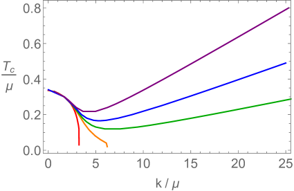
Figure 1: $T_{c}$ vs $k/\mu$ with $\tau\in\text{[}0,\,\text{}\frac{1}{\sqrt{3}}\frac{12}{10}]$ (red-purple).

In $k/\mu\ll 1$ region, one cannot find the $\tau$ effect on $T_{c}$, i.e., $T_{c}$ is independent on $\tau$ in the coherent regime ($k/\mu\rightarrow 0$). This would be consistent with the result at $k/\mu=0$ in Cremonini:2016bqw .

However, as $k/\mu$ is increased, we find two main features related to $\tau$. First, there would be a critical $\tau$, $\tau_{c}$, to study superconducting phases at $k/\mu\gg 1$ limit. For instance, if $\tau=\frac{1}{\sqrt{3}}\frac{8}{10}$ (orange) in Fig. 1, superconducting phases cannot be obtained in $k/\mu>6$ regime. Therfore, in order to study superconductors in the strong momentum relaxation limit ($k/\mu\rightarrow\infty$), we need to consider $\tau>\tau_{c}$. In this paper, we take $\tau_{c}=\frac{1}{\sqrt{3}}\frac{8}{10}$ for simplicity: in Fig. 1, one may try to find a more exact value for $\tau_{c}$ between the orange one ($\tau_{c}=\frac{1}{\sqrt{3}}\frac{8}{10}$) and the green one ($\tau_{c}=\frac{1}{\sqrt{3}}\frac{9}{10}$).

Second, at given $k/\mu$, $\tau$ enhances $T_{c}$ (e.g., from green to purple). This indicates that the superconducting instability can be triggered more easily at higher coupling $\tau$. Thus, a larger $\tau$ might be useful to investigate the superconducting phase at higher temperature, i.e., high $T_{c}$ superconductors.

High $T_{c}$ superconductor and linear-$T$ resistivity:

In summary, we find that the coupling $\tau$, $\tau>\tau_{c}$, would be important not only for superconducting phases at strong momentum relaxation region, but also for high $T_{c}$ superconductors.

Based on this result, we may argue that, in order to describe high $T_{c}$ superconductors having linear-$T$ resistivity (16) near $T_{c}$ (i.e., the region where the normal phase still can be useful), we may need the following conditions:

$$\text{i)}\,\,\tau>\tau_{c};\qquad\qquad\text{ii)}\,\,k/\mu\gg 1\,.$$ (31)

This would imply that the trivial coupling term $B(\phi)=M^{2}$ ($\tau=0$ case) used in most of the previous literature may not capture a complete feature of the superconducting phases at strong momentum relaxation limit. In the following section 3, we will study if the condition (31) can also be related to Homes’ law.

Instability condition for $M^{2}$:

We finish this section with the instability condition for $M^{2}$ with the complex scalar field equation of motion. Here we consider the scaling case ($\tau=\frac{1}{\sqrt{3}}$) because one can obtain a simple analytic instability condition with it.

At $\tau=\frac{1}{\sqrt{3}}$, the complex scalar field equation of motion in the IR geometry (20) can be expressed as

$$\Phi^{\prime\prime}(\rho)-\frac{1}{\rho}\Phi^{\prime}(\rho)+\frac{4Q^{2}\left(M^{2}(k^{2}-6Q^{2})\rho^{2}-2q^{2}(k^{2}-2Q^{2})\right)}{(k^{2}-6Q^{2})^{2}\rho^{4}}\,\Phi(\rho)=0\,,$$ (32)

and this equation can be solved analytically by the combination of Bessel functions $J_{\nu}$:

$$\Phi(\rho)=c_{1}\,\rho\,\Gamma(1-\nu)J_{-\nu}\left(\sqrt{\frac{8q^{2}Q^{2}(k^{2}-2Q^{2})}{(k^{2}-6Q^{2})^{2}}}\frac{1}{\rho}\right)\,+\,c_{2}\,\rho\,\Gamma(1+\nu)J_{\nu}\left(\sqrt{\frac{8q^{2}Q^{2}(k^{2}-2Q^{2})}{(k^{2}-6Q^{2})^{2}}}\frac{1}{\rho}\right)\,,$$ (33)

where the index $\nu$ is

$$\begin{split}\nu=\sqrt{\frac{k^{2}-(6+4M^{2})Q^{2}}{k^{2}-6Q^{2}}}\,.\end{split}$$ (34)

Then, the instability appears when the index $\nu$ of Bessel function becomes imaginary. Note that, unlike the case of $k=0$ in Cremonini:2016bqw , there are two ways to make the imaginary $\nu$ depending on the sign of the numerator (or denominator) in $\nu$: i) the positive numerator with the negative denominator; ii) the negative numerator with the positive denominator. Each case produces the following instability condition for $M^{2}$

$$\begin{split}M^{2}<\frac{k^{2}-6Q^{2}}{4Q^{2}}<0\qquad\text{or}\qquad M^{2}>\frac{k^{2}-6Q^{2}}{4Q^{2}}>0\,.\end{split}$$ (35)

Note that only the first condition in (35) is consistent at $k=0$. Thus, from the perspective of continuity encompassing the $k=0$ case, the first condition in (35) might be the proper instability condition.

3 Homes’ law

In this section, considering the coupling (26), we study Homes’ law with the fully back-reacted geometry.

3.1 Setup for numerics

We consider the following ansatz to obtain the fully back-reacted background solutions

$$\begin{split}&\mathrm{d}s^{2}=\frac{1}{\tilde{z}^{2}}\left[-(1-\tilde{z})U(\tilde{z})\mathrm{d}\tilde{t}^{2}+\frac{\mathrm{d}\tilde{z}^{2}}{(1-\tilde{z})U(\tilde{z})}+V(\tilde{z})\mathrm{d}\tilde{x}^{2}+V(\tilde{z})\mathrm{d}\tilde{y}^{2}\right]\,,\\ &A=(1-\tilde{z})a(\tilde{z})\mathrm{d}\tilde{t}\,,\quad\phi=\frac{\sqrt{3}}{2}\log[1+\varphi(\tilde{z})]\,,\quad\Phi=\tilde{z}^{\Delta_{-}}\,\eta(\tilde{z}),\\ &\psi_{1}=\tilde{k}\,\tilde{x}\,,\quad\psi_{2}=\tilde{k}\,\tilde{y}\,,\end{split}$$ (36)

where

$$\tilde{z}:=\frac{z}{z_{h}}\,,\qquad\tilde{t}:=\frac{t}{z_{h}}\,,\qquad\tilde{x}:=\frac{x}{z_{h}}\,,\qquad\tilde{y}:=\frac{y}{z_{h}}\,,\qquad\mbox{${\tilde{k}}$}:=k\,z_{h}\,.$$ (37)

Here $U,V,a,\varphi$ and $\eta$ are functions of the holographic direction $\tilde{z}$. In this coordinate, the AdS boundary is located at $\tilde{z}=0$ and the horizon is at $\tilde{z}=1$. Note that the coordinate (36) is related to (8) with $z=1/r$ and the form of ansatz (36) is chosen for the convenience of numerical analysis for superconducting phase.

With the ansatz (36), one can identify the Hawking temperature $T$ and the chemical potential $\mu$ as

$$T=\frac{g_{tt}^{\prime}(\tilde{z})}{4\pi\sqrt{g_{tt}g_{\tilde{z}\tilde{z}}}}\Bigr{|}_{\tilde{z}=1}=\frac{U(1)}{4\pi}\,,\quad\mu=A_{t}(0)=a(0)\,,$$ (38)

and the condensate $\Phi^{(+)}$ in (30) can be read off from $\eta$ in (36) near the AdS boundary as

$$\begin{split}\Phi=\Phi^{(-)}\,\tilde{z}^{\Delta_{-}}\,+\,\Phi^{(+)}\,\tilde{z}^{\Delta_{+}}\,+\,\dots\quad\Leftrightarrow\quad\eta=\Phi^{(-)}\,+\,\Phi^{(+)}\,\tilde{z}^{\Delta_{+}-\Delta_{-}}\,+\,\dots\,,\end{split}$$ (39)

where $\Delta_{\pm}$ is defined in (30).

In order for the superconducting phases, we set the source $\Phi^{(-)}=0$, i.e., $\eta(0)=0$ and need to find the state with the finite condensate $\Phi^{(+)}\neq 0$. One can find such a state by solving the equations (3)-(7) numerically with the ansatz (36). The typical condensate is plotted in Fig. 2: the condensate tends to be enhanced with increasing $k/\mu$ and this seems to be a generic feature of holographic superconductors in the presence of the momentum relaxation.

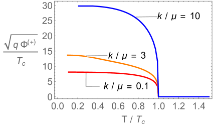
Figure 2: Condensation vs temperature at $\tau=1/\sqrt{3}$ where $T_{c}$ is the critical temperature.

In what follows, in section 3.2, we focus on the scaling case $\tau=1/\sqrt{3}>\tau_{c}$ and study the electric optical conductivity $\sigma(\omega)$ and the superfluid density $\rho_{s}$. Then, using the results in section 3.2, we investigate Homes’ law in section 3.3. In section 3.4, we discuss the $\tau$ effect on Homes’ law.

3.2 Electric conductivity and superfluid density

Let us study the electric optical conductivity of the holographic model (2). From here on, we use the scaled variables (37) without tilde for simplicity.

Holographic electric optical conductivity:

In order to compute the electric optical conductivity, we need to consider the following fluctuations:

$$\begin{split}\delta g_{tx}=h_{tx}(z)\,e^{-i\omega t}\,,\qquad\delta A_{x}=a_{x}(z)\,e^{-i\omega t}\,,\qquad\delta\psi_{x}=\xi_{x}(z)\,e^{-i\omega t}\,,\end{split}$$ (40)

where the fluctuations behave near the AdS boundary as

$$\begin{split}h_{tx}(z)&\,=\,\frac{h_{tx}^{(S)}}{z^{2}}\,+\,h_{tx}^{(R)}\,+\,\dots\,,\\ a_{x}(z)&\,=\,a_{x}^{(S)}\,\,\,+\,\,a_{x}^{(R)}\,z\,+\,\dots\,,\\ \xi_{x}(z)&\,=\,\xi_{x}^{(S)}\,\,\,+\,\,\xi_{x}^{(R)}\,z\,+\,\dots\,,\end{split}$$ (41)

here the leading coefficients ($h_{tx}^{(S)},a_{x}^{(S)},\xi_{x}^{(S)}$) correspond to the sources, and the subleading terms ($h_{tx}^{(R)},a_{x}^{(R)},\xi_{x}^{(R)}$) would be interpreted as the response by the holographic dictionary.

The electric optical conductivity can be obtained by the Kubo formula in terms of the boundary coefficients in (41):

$$\begin{split}\sigma(\omega)=\frac{1}{i\omega}G_{j^{x}j^{x}}^{R}(\omega)=\frac{a_{x}^{(R)}}{i\omega\,a_{x}^{(S)}}\,,\end{split}$$ (42)

where $G_{j^{x}j^{x}}^{R}$ is the current-current retarded Green’s function. The second equality in (42) holds when $a_{x}^{(S)}$ is the only non-zero source.

In order to make the source-vanishing boundary condition except $a_{x}^{(S)}$, one may use the diffeomorphisms and gauge-transformations Kim:2015sma ; Donos:2013eha . With a constant residual gauge parameter $\zeta$ fixing $\delta g_{rx}=0$ Kim:2015sma , it can be shown that the fluctuations in (40) except $\delta A_{x}$ can be expanded near the AdS boundary as

$$\begin{split}z^{2}\,\delta{g_{tx}}\,\sim\,(h_{tx}^{(S)}-i\omega\zeta)e^{-i\omega t}\,=\,0\,,\qquad\delta\psi_{x}\,\sim\,(\xi_{x}^{(S)}+k\zeta)e^{-i\omega t}\,=\,0\,,\end{split}$$ (43)

where the equalities correspond to the source-vanishing boundary condition except $a_{x}^{(S)}$. Plugging one of the equations in (43) into the other, (43) produces a single condition

$$\begin{split}\xi_{x}^{(S)}-\frac{ik}{\omega}h_{tx}^{(S)}=0\,.\end{split}$$ (44)

Therefore, one can use (42) to study the electric optical conductivity by solving the equation of motion of the fluctuations with the boundary condition (44).

Electric optical conductivity in strange metal/superconductor transition:

Using the method above, we make the plot of the optical conductivity in Fig. 3.

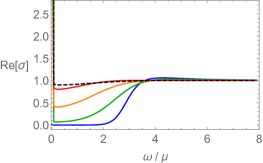
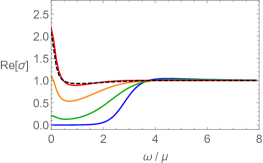
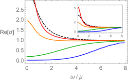
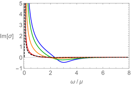
(a) $k/\mu=0.1,\ \ T/T_{c}=1.5,1,0.93,$ $0.75,0.21$ (dashed, red, orange, green, blue)

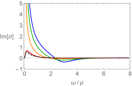
(b) $k/\mu=1,\ \ T/T_{c}=1.5,1,0.93,$ $0.75,0.21$ (dashed, red, orange, green, blue)

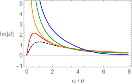
(c) $k/\mu=10,\ \ T/T_{c}=1.5,1,0.97,$ $0.87,0.35$ (dashed, red, orange, green, blue)

Figure 3: Electric conductivity with various $k/\mu=0.1,1$ and $10$. The first row displays Re$[\sigma(\omega)]$, while Im$[\sigma(\omega)]$ is plotted in the second row ($\tau=1/\sqrt{3}$).

The color of curves denotes a temperature ratio $T/T_{c}$: the dashed black is for the normal metal phase ($T>T_{c}$), the red line is for the critical temperature ($T=T_{c}$), and other colors (from orange to blue) correspond to the superconducting phase ($T<T_{c}$).

For $T\geq T_{c}$, one can see that the DC conductivity, $\sigma(\omega=0)$, is finite due to the momentum relaxation, while the superconducting phase ($T<T_{c}$) produces $1/\omega$ pole in Im$[\sigma]$ giving the infinite DC conductivity. By the Kramers-Kronig relation, $1/\omega$ pole in Im$[\sigma]$ implies that Re$[\sigma]$ has a delta function at $\omega=0$: this is one of hallmarks of holographic superconductor.

Let us make some further comments on the electric conductivity of our model (2). In holography, there are two simple gravity models to study the electric conductivity of the normal phase in the presence of the momentum relaxation: i) the linear axion model Andrade:2013gsa ; ii) the Gubser-Rocha model with the axion field (2).

In Kim:2015dna , using the linear axion model, the authors studied the optical conductivity with the phase transition between the normal phase and the superconducting phase. Thus, it would be instructive to compare the features in Fig. 3 and the result in Kim:2015dna . To our knowledge, our work is the first holographic study considering the optical conductivity of (2) for the normal phase ($\Phi=0$), i.e., the Gubser-Rocha model with the axion field.

We found one distinct feature between two holographic models at strong momentum relaxation region: unlike the linear axion model Kim:2015dna , at large $k/\mu$, the Drude like peak in the normal phase does not disappear for the Gubser Rocha model (e.g., see dashed black (and red) line in Fig. 3(c)). In order to show this feature more clearly at strong momentum relaxation limit ($k/\mu\rightarrow\infty$), we take $\mu/k=0$ and make the plot of the optical conductivity in Fig. 4(a).

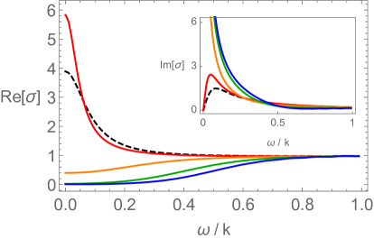
(a) $\sigma(\omega)$ vs $\omega/k$. The inset is Im $\sigma$.

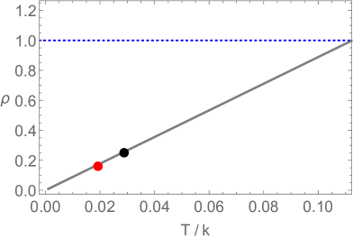
(b) $\rho$ vs $T/k$.

Figure 4: The electic conductivity at $\mu/k=0$. Left: $\sigma(\omega)$ of the Gubser-Rocha model at $T/T_{c}=1.5,1,0.93,$ $0.75,0.41$ (dashed, red, orange, green, blue). Right: The DC resistivity $\rho$ ($1/\sigma(\omega=0)$) of two holographic models: the Gubser Rocha model (solid gray) (45), the linear axion model (dotted blue) (46). The black (red) dot corresponds to the DC limit of the black (red) line in Fig. 4(a): it shows that the numerical result of $\sigma(\omega=0)$ is consistent with the analytic DC result.

The non-vanishing Drude like peak in the strong momentum relaxation limit might be related to the fact that the Gubser-Rocha model produces linear-$T$ resistivity unlike the linear axion model. For instance, at $\mu/k=0$, both holographic models show the DC conductivity as

$$\sigma_{DC}=\sqrt{1+\tilde{Q}}\left(1+\frac{\mu^{2}}{k^{2}}\right)\,\sim\,\sqrt{1+\tilde{Q}}\,\sim\,\frac{k}{2\sqrt{2}\pi T}\,,\,\,\quad\text{(Gubser-Rocha model)}$$ (45)

$$\sigma_{DC}=1+\frac{\mu^{2}}{k^{2}}\,\sim\,1\,,\qquad\qquad\qquad\qquad\qquad\qquad\quad\quad\,\,\,\text{(Linear axion model)}$$ (46)

where ${\tilde{Q}}$ from the dilaton field plays an important role for the linear-$T$ resistivity.

In Fig. 4(b), we display the DC conductivity of two holographic models: the Gubser Rocha model (solid gray) (45), the linear axion model (dotted blue) (46). The black (red) dot in Fig. 4(b) corresponds to the DC limit of the black (red) line in Fig. 4(a): it shows that the numerically computed $\sigma(\omega=0)$ is consistent with the analytic DC result.

Note that, at $\omega/k\rightarrow\infty$, $\sigma(\omega)=1$ in both models. However, in the opposite limit, $\omega/k\rightarrow 0$, the linear axion model gives the constant value, i.e., $\sigma(\omega)=1$ (46) unlike the Gubser-Rocha model (45). Thus, for the linear axion model, the optical conductivity of the normal phase would be a constant, $\sigma(\omega)=1$, in all $\omega$ regime without producing a Drude like peak.

Two-fluid model and superfluid density:

For superconducting phase (roughly $0.5<T/T_{c}<1$) in Fig. 3, Re$[\sigma]$ also has a remaining finite value at $\omega=0$ in addition to the delta function by the Kramers-Kronig relation. This residual Drude-like peak may be interpreted by the two-fluid model Horowitz:2013jaa as a contribution from the normal component in the superconducting phase, which has also been observed in other holographic superconductor models such as linear-axion model Kim:2015dna , Q-lattice model Ling:2014laa , and Helical lattice model Erdmenger:2015qqa .

The two-fluid model demonstrates that the low frequency behavior of the optical conductivity can be fitted with the following formula:

$$\sigma(\omega)\,=\,i\,\frac{\rho_{s}}{\omega}\,+\,\frac{\rho_{n}\,\tau_{r}}{1-i\,\omega\,\tau_{r}}\,+\,\rho_{0}\,,$$ (47)

where $\rho_{s}$ and $\rho_{n}$ are defined as the superfluid density and the normal fluid density. $\tau_{r}$ is the relaxation time. $\rho_{0}$ may be related to the pair creation and can be used to fit the numerical data in the presence of the momentum relaxation Kim:2015dna .

The superfluid density $\rho_{s}$ is our main interest to study Homes’ law, which can be read off from the fitting curve (47). One interesting feature of $\rho_{s}$ in holographic superconductors Kim:2016jjk ; Erdmenger:2012ik ; Kim:2016hzi ; Erdmenger:2015qqa is that there is a finite gap at $T=0$ between $\rho_{s}$ and the charge density $n$ in the presence of the momentum relaxation. This also happens in our superconductor model. See Fig. 5. Thus, this non-vanishing gap at finite $k/\mu$ seems to be a generic feature of holographic superconductors.

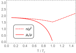
(a) $k/\mu=0.1$

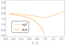
(b) $k/\mu=1$

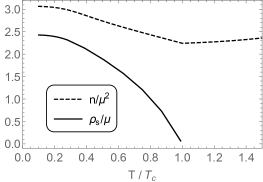
(c) $k/\mu=3$

Figure 5: The charge density $n$, superfluid density $\rho_{s}$ vs $T/T_{c}$. The gap between $n$ and $\rho_{s}$ at $T=0$ opens at finite $k/\mu$ ($\tau=1/\sqrt{3}$).

We also find that, as $T$ is lowered, $\rho_{0}$ and $\rho_{n}$ are reduced while $\rho_{s}$ is enhanced. For the relaxation time $\tau_{r}$, we find it is decreasing as $T$ is lowered. The behavior of $\tau_{r}$, at low $T$ depends on holographic models: it is increasing in Horowitz:2013jaa , it is decreasing first and then increasing in Ling:2014laa . So, apparently, the more detailed analysis and the unified description for the relaxation time for holographic superconductor is still needed. We leave this subject as future work.

3.3 Homes’ law at strong momentum relaxation

Now let us discuss Homes’ law (1). Computing three quantities ($\rho_{s}(T=0)$, $T_{c}$, $\sigma_{DC}(T_{c})$) as a function of $k/\mu$, we may check Homes’ law at given $\tau$.

Note that $\rho_{s}(T=0)$ can be read off from (47) in principle. However, as one can see from Fig. 5, $\rho_{s}(T)$ does not reach to $T=0$ due to the instability in our numerics. Thus, we extrapolate $\rho_{s}(T)$ up to zero temperature in order to obtain $\rho_{s}(T=0)$. Other quantity for Homes’ law, $\sigma_{DC}(T_{c})$, is determined by (14) with a numerically computed $T_{c}$.

We first study Homes’ law for the scaling case ($\tau=1/\sqrt{3}$). In Fig. 6, we display ($\rho_{s}(T=0)$, $T_{c}$, $\sigma_{DC}(T_{c})$).

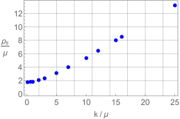
(a) $\rho_{s}/\mu$ at $T=0$

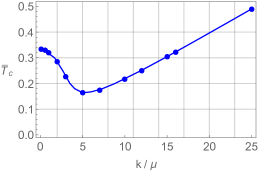
(b) $T_{c}/\mu$

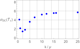
(c) $\sigma_{DC}$

Figure 6: $\rho_{s},T_{c},$ and $\sigma_{DC}(T_{c})$ for $\tau=1/\sqrt{3}$. $\bar{T}_{c}$ is the shorthand notation for $T_{c}/\mu$. The blue solid line corresponds to the one in Fig. 1.

As we increase $k/\mu$, in the strong momentum relaxation regime, one can see that $\rho_{s}$ and $T_{c}$ are increasing linearly while $\sigma_{DC}$ saturates to some constant.

Unlike the behavior of $\rho_{s}$ and $\sigma_{DC}$, the increasing behavior of $T_{c}$ is the distinct property not observed in other holographic studies, for instance, $T_{c}$ tends to decrease or saturates to some value in Erdmenger:2015qqa ; Kim:2016jjk ; Kim:2016hzi . Moreover, this increasing feature from $T_{c}$ seems to play an important role for Homes’ law as we show in shortly.

Homes’ law with linear-$T$ resistivity:

Using the data in Fig. 6, we make a plot of the ratio $\rho_{s}/(\sigma_{DC}T_{c})$ ($=:C$) as a function of $k/\mu$ in Fig. 7(b), and observe that the ratio $C$ becomes a constant, $C\sim 4.7$, at $k/\mu\gg 1$ limit, i.e., Homes’ law (1) appears to hold in the strong momentum relaxation limit.

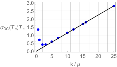
(a) $\sigma_{DC}T_{c}$ vs $k/\mu$

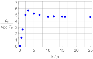
(b) Homes’ law

Figure 7: Left: $\sigma_{DC}T_{c}$ vs $k$. $\bar{T}_{c}$ is the shorthand notation for $T_{c}/\mu$. The black solid line is (48). Right: Checking Homes’ law: Homes’ law appears to hold in the strong momentum relaxation limit.

One may wonder if $C$ remains a constant at $k/\mu>25$ in Fig. 7(b). Evaluating $C$ at $\mu/k=0$, we confirmed that $C$ is a constant around $4.7$ in $k/\mu\gg 1$ limit.

Homes’ law at strong momentum relaxation limit, the constant $C$, can be viewed as the cancelation of the two linearities in $k/\mu$: one from $\rho_{s}$ in Fig. 6(a) and the other from $\sigma_{DC}T_{c}$ in Fig. 7(a). The linearity in Fig. 7(a), the black solid line, can be understood by

$$\sigma_{DC}\,\frac{T}{\mu}\,=\,\frac{1}{2\sqrt{2}\pi}\,\frac{k}{\mu}\,,$$ (48)

where the DC conductivity formula (16) is used. Note that linear-$T$ resistivity in (16) plays a crucial role because (48) becomes $T$-independent so valid at $T\gtrsim T_{c}$. Alternatively, the linearity in Fig. 7(a) (or (48)) may be understood from the fact that $T_{c}$ is linear in $k$ (Fig. 6(b)) and $\sigma_{DC}$ is constant (Fig. 6(c)).

3.4 The coupling $\tau$ dependence

Next, let us discuss the $\tau$ dependence in Homes’ law. We display the plots for ($\rho_{s}(T=0)$, $T_{c}$, $\sigma_{DC}(T_{c})$) with various $\tau$ in Fig. 8:

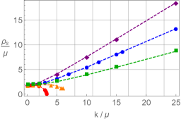
(a) $\rho_{s}/\mu$ at $T=0$

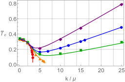
(b) $T_{c}/\mu$

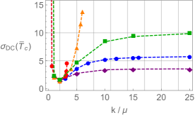
(c) $\sigma_{DC}$

Figure 8: $\rho_{s}/\mu,T_{c}/\mu,$ and $\sigma_{DC}$ for $\tau=(0,\,\frac{1}{\sqrt{3}}\frac{8}{10},\,\frac{1}{\sqrt{3}}\frac{9}{10},\,\frac{1}{\sqrt{3}}\frac{10}{10},\,\frac{1}{\sqrt{3}}\frac{12}{10})$ (red, orange, green, blue, purple). $\bar{T}_{c}$ is the shorthand notation for $T_{c}/\mu$. The solid lines in (b) are Fig. 1 and the dashed lines in (a), (c) are fitting curves.

blue dots in Fig. 8 correspond to Fig. 6 (i.e., the scaling case $\tau=1/\sqrt{3}$).

$\rho_{s}$ and $T_{c}$ with $\tau$:

$\rho_{s}(T=0)$ in Fig. 8(a) shows the qualitatively similar behavior with $T_{c}$ in Fig. 8(b): as we increase $k/\mu$, at $\tau<\tau_{c}$ (red, orange), it is reduced while, at $\tau>\tau_{c}$ (green, blue, purple), it is linearly increasing. One may understand the resemblance between $\rho_{s}(T=0)$ and $T_{c}$ as follows. As can be seen in Fig. 5, $\rho_{s}(T)$ is zero at $T=T_{c}$ and monotonically increasing at $T<T_{c}$. Thus, in order to have a large (small) $\rho_{s}$ at $T=0$, $T_{c}$ may need to be large (small) as well, i.e., $\rho_{s}(T=0)\sim T_{c}$.

Note that the solid lines in Fig. 8(b) are Fig. 1, i.e., $T_{c}$ from the fully back-reacted geometry is consistent with the one without back-reaction. This may imply that $\rho_{s}$ might also be understood in the probe limit. If one can develop the methodology to compute $\sigma(\omega)$ only with the IR geometry (the $T=0$ analysis), we suspect that the numerical result in Fig. 8(a) might also be confirmed in a simple probe limit with the scaling property (22).

$\sigma_{DC}(T_{c})$ with $\tau$:

In Fig. 8(c), unlike $\rho_{s}$, there is no resemblance between $\sigma_{DC}(T_{c})$ and $T_{c}$. At small $k/\mu$, $\sigma_{DC}$ is diverging independent of $\tau$, which reflects the fact the conductivity is infinite at zero momentum relaxation.

On the other hand, at larger $k/\mu$, one can see the $\tau$ dependence on $\sigma_{DC}(T_{c})$. At $\tau<\tau_{c}$ (red, orange), it is increasing while, at $\tau>\tau_{c}$ (green, blue, purple), it saturates to some constant. Note that the behavior of $\sigma_{DC}(T_{c})$ at large $k/\mu$ depends on the holographic models: for instance, it is increasing in the Q-lattice model Kim:2016jjk or saturated in the linear axion model Kim:2016hzi .

Homes’ law at $\tau>\tau_{c}$:

With the data in Fig. 8, we find Homes’ law (1) at the strong momentum relaxation limit for $\tau>\tau_{c}$ (green, blue, purple): i.e., $C$ become a constant at $k/\mu\gg 1$. See Fig. 9(b).

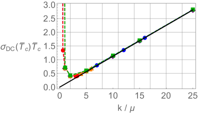
(a) $\sigma_{DC}T_{c}$ vs $k/\mu$

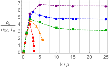
(b) Homes’ law

Figure 9: Left: $\sigma_{DC}T_{c}$ vs $k$. The black solid line is (48). Right: Checking Homes’ law with $\tau=(0,\,\frac{1}{\sqrt{3}}\frac{8}{10},\,\frac{1}{\sqrt{3}}\frac{9}{10},\,\frac{1}{\sqrt{3}}\frac{10}{10},\,\frac{1}{\sqrt{3}}\frac{12}{10})$ (red, orange, green, blue, purple).

As did in the scaling case ($\tau=1/\sqrt{3}$) in Fig. 7(a), Homes’ law at $\tau>\tau_{c}$ can be understood from the cancelation of the two linearities in $k/\mu$: one from $\rho_{s}$ (Fig. 8(a)) and the other from the linear-$T$ resistivity (Fig. 9(a)).

We also find that the saturating value of $C$ depends on the value of $\tau$. Thus, $\tau$ might be used to match the experiment data: $C=4.4$ for ab-plane high $T_{c}$ superconductors as well as clean BCS superconductors and $C=8.1$ for c-axis high $T_{c}$ superconductor and BCS superconductors in the dirty limit.

4 Conclusions

We have investigated Homes’ law (1) by computing the critical temperature $T_{c}$, the superfluid density $\rho_{s}$ at zero temperature, and the DC conductivity $\sigma_{DC}$ at $T_{c}$ in a holographic superconductor based on the Gubser-Rocha model (2) with the minimally chosen coupling term $B(\phi)$:

$$B(\phi)=M^{2}\,\cosh\left(\tau\phi\right)\,,$$ (49)

where it corresponds to the mass term of the complex scalar field, $M^{2}$, at $\tau=0$. The action (2) also contains the axion field to study the momentum relaxation where its strength is denoted as $k/\mu$. In this setup, Homes’ law means that $C:=\rho_{s}/(\sigma_{DC}T_{c})$ is independent of the momentum relaxation.

The Gubser-Rocha model, a normal phase, is appealing in that the linear-$T$ resistivity can be obtained at strong momentum relaxation limit ($k/\mu\gg 1$) above $T_{c}$. Considering the complex scalar field with the Gubser-Rocha model, we find that, in order to study the superconducting phase at $k/\mu\gg 1$, $\tau$ in the coupling (49) is important. We show that the conditions to study a holographic superconductor having the linear-$T$ resistivity above $T_{c}$ would be:

$$\text{i)}\,\,\tau>\tau_{c};\qquad\qquad\text{ii)}\,\,k/\mu\gg 1\,,$$ (50)

where $\tau_{c}\neq 0$ can be determined numerically from the instability analysis for $T_{c}$. The first condition i) in (50) means that if $\tau$ is smaller than $\tau_{c}$ the superconducting phase does not exist at large $k/\mu$. In particular, the trivial coupling term $B(\phi)=M^{2}$ ($\tau=0$ case), the mass term of the complex scalar field, used in previous literature can not capture a complete feature of the superconducting phase at $k/\mu\gg 1$.

With the condition (50), we find Homes’ law can hold in the strong momentum relaxation limit, i.e., $C$ becomes a constant at $k/\mu\gg 1$ limit. In Hartnoll:2014lpa , it is argued that if the momentum is relaxed quickly(strongly), which is an extrinsic so non-universal effect, transport can be governed by an intrinsic and universal effect such as diffusion of energy and charge. Thus, the universality of linear-$T$ resistivity may appear in the regime of strong momentum relaxation (so called the incoherent regime). Consequently, Homes’ law can appear also in the strong momentum relaxation limit.

Furthermore, we showed that Homes’ law at $k/\mu\gg 1$ can be understood from the cancelation of the two linearities in $k/\mu$: one from $\rho_{s}(T=0)$ (numerical result) and the other from the linear-$T$ resistivity (analytic result) (48). It will be interesting to show the linearity of $\rho_{s}(T=0)$ in $k/\mu$ also analytically. If one can develop the method to compute the optical conductivity with the IR geometry ($T=0$ analysis) in the superconducting phase, we suspect that the linearity of $\rho_{s}(T=0)$ in $k/\mu$ might be related with the IR scaling property of the coupling $B(\phi)$ (22).

We find that the value of $C$ at $k/\mu\gg 1$ depends on the value of $\tau$ so $\tau$ can be used to match the experiment data: $C=4.4$ for ab-plane high $T_{c}$ superconductors as well as clean BCS superconductors and $C=8.1$ for c-axis high $T_{c}$ superconductor and BCS superconductors in the dirty limit.

It may also be interesting to study Homes’ law with the holographic models having other IR geometries Gouteraux:2014hca ; Ahn:2017kvc ; Ahn:2019lrh together with linear $T$ resistivity. In Ahn:2019lrh , authors found that when the IR geometry is governed by a finite dynamical exponent $z$ and a hyperscaling violating exponent $\theta$ unlike the Gubser-Rocha model ($z\rightarrow\infty$, $\theta\rightarrow-\infty$), the linear-$T$ resistivity can also exhibit at high temperature if the momentum relaxation is strong. Therefore, one may investigate how much general our results in this paper are. One may also check if $\tau>\tau_{c}$ condition in (50) is necessary for Homes’ law in more generic setup. We leave these subjects as future work and hope to address them in the near future.

- (1) S. A. Hartnoll, A. Lucas and S. Sachdev, Holographic quantum matter, 1612.07324.
- (2) J. Zaanen, Y.-W. Sun, Y. Liu and K. Schalm, Holographic Duality in Condensed Matter Physics. Cambridge Univ. Press, 2015.
- (3) M. Ammon and J. Erdmenger, Gauge/gravity duality. Cambridge Univ. Pr., Cambridge, UK, 2015.
- (4) M. Baggioli, Applied Holography: A Practical Mini-Course. SpringerBriefs in Physics. Springer, 2019, 10.1007/978-3-030-35184-7.
- (5) S. A. Hartnoll, Lectures on holographic methods for condensed matter physics, Class.Quant.Grav. 26 (2009) 224002, [0903.3246].
- (6) C. P. Herzog, Lectures on Holographic Superfluidity and Superconductivity, J.Phys.A A42 (2009) 343001, [0904.1975].
- (7) C. C. Homes, S. V. Dordevic, T. Valla and M. Strongin, Scaling of the superfluid density in high-temperature superconductors, Phys. Rev. B 72, 134517 (2005) (8, [cond-mat/0410719].
- (8) C. Homes, S. Dordevic, M. Strongin, D. Bonn, R. Liang et al., Universal scaling relation in high-temperature superconductors, Nature 430 (2004) 539, [cond-mat/0404216].
- (9) S. A. Hartnoll, C. P. Herzog and G. T. Horowitz, Building a Holographic Superconductor, Phys.Rev.Lett. 101 (2008) 031601, [0803.3295].
- (10) S. A. Hartnoll, C. P. Herzog and G. T. Horowitz, Holographic Superconductors, JHEP 0812 (2008) 015, [0810.1563].
- (11) G. T. Horowitz, Introduction to Holographic Superconductors, 1002.1722.
- (12) R.-G. Cai, L. Li, L.-F. Li and R.-Q. Yang, Introduction to Holographic Superconductor Models, Sci. China Phys. Mech. Astron. 58 (2015) 060401, [1502.00437].
- (13) K. Y. Kim and M. Taylor, Holographic d-wave superconductors, JHEP 08 (2013) 112, [1304.6729].
- (14) B. Goutéraux and E. Mefford, Normal charge densities in quantum critical superfluids, Phys. Rev. Lett. 124 (2020) 161604, [1912.08849].
- (15) B. Goutéraux and E. Mefford, Non-vanishing zero-temperature normal density in holographic superfluids, JHEP 11 (2020) 091, [2008.02289].
- (16) D. Arean, M. Baggioli, S. Grieninger and K. Landsteiner, A Holographic Superfluid Symphony, 2107.08802.
- (17) A. Donos, P. Kailidis and C. Pantelidou, Dissipation in holographic superfluids, JHEP 09 (2021) 134, [2107.03680].
- (18) M. Ammon, D. Arean, M. Baggioli, S. Gray and S. Grieninger, Pseudo-spontaneous Symmetry Breaking in Hydrodynamics and Holography, 2111.10305.
- (19) G. T. Horowitz, J. E. Santos and D. Tong, Optical Conductivity with Holographic Lattices, JHEP 1207 (2012) 168, [1204.0519].
- (20) D. Vegh, Holography without translational symmetry, 1301.0537.
- (21) A. Donos and J. P. Gauntlett, Holographic Q-lattices, JHEP 1404 (2014) 040, [1311.3292].
- (22) T. Andrade and B. Withers, A simple holographic model of momentum relaxation, JHEP 1405 (2014) 101, [1311.5157].
- (23) A. Donos and S. A. Hartnoll, Interaction-driven localization in holography, Nature Phys. 9 (2013) 649–655, [1212.2998].
- (24) J. Erdmenger, B. Herwerth, S. Klug, R. Meyer and K. Schalm, S-Wave Superconductivity in Anisotropic Holographic Insulators, JHEP 05 (2015) 094, [1501.07615].
- (25) G. T. Horowitz and J. E. Santos, General Relativity and the Cuprates, 1302.6586.
- (26) H. B. Zeng and J.-P. Wu, Holographic superconductors from the massive gravity, Phys.Rev. D90 (2014) 046001, [1404.5321].
- (27) Y. Ling, P. Liu, C. Niu, J.-P. Wu and Z.-Y. Xian, Holographic Superconductor on Q-lattice, JHEP 02 (2015) 059, [1410.6761].
- (28) T. Andrade and S. A. Gentle, Relaxed superconductors, 1412.6521.
- (29) K.-Y. Kim, K. K. Kim and M. Park, A Simple Holographic Superconductor with Momentum Relaxation, JHEP 04 (2015) 152, [1501.00446].
- (30) M. Baggioli and M. Goykhman, Phases of holographic superconductors with broken translational symmetry, JHEP 07 (2015) 035, [1504.05561].
- (31) M. Baggioli and M. Goykhman, Under The Dome: Doped holographic superconductors with broken translational symmetry, JHEP 01 (2016) 011, [1510.06363].
- (32) K. K. Kim, M. Park and K.-Y. Kim, Ward identity and Homes’ law in a holographic superconductor with momentum relaxation, JHEP 10 (2016) 041, [1604.06205].
- (33) K.-Y. Kim and C. Niu, Homes’ law in Holographic Superconductor with Q-lattices, JHEP 10 (2016) 144, [1608.04653].
- (34) Y. Ling and X. Zheng, Holographic superconductor with momentum relaxation and Weyl correction, Nucl. Phys. B917 (2017) 1–18, [1609.09717].
- (35) H.-S. Jeong, K.-Y. Kim and C. Niu, Linear- resistivity at high temperature, JHEP 10 (2018) 191, [1806.07739].
- (36) J. Erdmenger, P. Kerner and S. Muller, Towards a Holographic Realization of Homes’ Law, JHEP 1210 (2012) 021, [1206.5305].
- (37) K.-Y. Kim, K. K. Kim, Y. Seo and S.-J. Sin, Coherent/incoherent metal transition in a holographic model, JHEP 12 (2014) 170, [1409.8346].
- (38) K.-Y. Kim, K. K. Kim, Y. Seo and S.-J. Sin, Gauge Invariance and Holographic Renormalization, Phys. Lett. B749 (2015) 108–114, [1502.02100].
- (39) K.-Y. Kim, K. K. Kim, Y. Seo and S.-J. Sin, Thermoelectric Conductivities at Finite Magnetic Field and the Nernst Effect, JHEP 07 (2015) 027, [1502.05386].
- (40) H.-S. Jeong, K.-Y. Kim, Y. Seo, S.-J. Sin and S.-Y. Wu, Holographic Spectral Functions with Momentum Relaxation, Phys. Rev. D 102 (2020) 026017, [1910.11034].
- (41) M. Baggioli, K.-Y. Kim, L. Li and W.-J. Li, Holographic Axion Model: a simple gravitational tool for quantum matter, Sci. China Phys. Mech. Astron. 64 (2021) 270001, [2101.01892].
- (42) S. S. Gubser and F. D. Rocha, Peculiar properties of a charged dilatonic black hole in , Phys.Rev. D81 (2010) 046001, [0911.2898].
- (43) R. A. Davison, K. Schalm and J. Zaanen, Holographic duality and the resistivity of strange metals, Phys. Rev. B89 (2014) 245116, [1311.2451].
- (44) Z. Zhou, Y. Ling and J.-P. Wu, Holographic incoherent transport in Einstein-Maxwell-dilaton Gravity, Phys. Rev. D94 (2016) 106015, [1512.01434].
- (45) K.-Y. Kim and C. Niu, Diffusion and Butterfly Velocity at Finite Density, JHEP 06 (2017) 030, [1704.00947].
- (46) Y. Liu and X.-M. Wu, Breakdown of hydrodynamics from holographic pole collision, 2111.07770.
- (47) J. Zaanen, Superconductivity: Why the temperature is high, Nature 430 (07, 2004) 512–513.
- (48) S. A. Hartnoll, Theory of universal incoherent metallic transport, Nature Phys. 11 (2015) 54, [1405.3651].
- (49) A. Lucas, S. Sachdev and K. Schalm, Scale-invariant hyperscaling-violating holographic theories and the resistivity of strange metals with random-field disorder, Phys. Rev. D 89 (2014) 066018, [1401.7993].
- (50) S. Cremonini and L. Li, Criteria For Superfluid Instabilities of Geometries with Hyperscaling Violation, JHEP 11 (2016) 137, [1606.02745].
- (51) R. A. Davison, Momentum relaxation in holographic massive gravity, Phys.Rev. D88 (2013) 086003, [1306.5792].
- (52) M. Blake and D. Tong, Universal Resistivity from Holographic Massive Gravity, Phys.Rev. D88 (2013) 106004, [1308.4970].
- (53) M. Blake, D. Tong and D. Vegh, Holographic Lattices Give the Graviton a Mass, Phys.Rev.Lett. 112 (2014) 071602, [1310.3832].
- (54) A. Donos and J. P. Gauntlett, Thermoelectric DC conductivities from black hole horizons, JHEP 11 (2014) 081, [1406.4742].
- (55) B. Goutéraux, Charge transport in holography with momentum dissipation, JHEP 1404 (2014) 181, [1401.5436].
- (56) Y. Ahn, H.-S. Jeong, D. Ahn and K.-Y. Kim, Linear- resistivity from low to high temperature: axion-dilaton theories, JHEP 04 (2020) 153, [1907.12168].
- (57) Y. Ling, C. Niu, J.-P. Wu and Z.-Y. Xian, Holographic Lattice in Einstein-Maxwell-Dilaton Gravity, JHEP 1311 (2013) 006, [1309.4580].
- (58) G. T. Horowitz and M. M. Roberts, Zero Temperature Limit of Holographic Superconductors, JHEP 0911 (2009) 015, [0908.3677].
- (59) P. Basu, Low temperature properties of holographic condensates, JHEP 03 (2011) 142, [1101.0215].
- (60) R.-Q. Yang, H.-S. Jeong, C. Niu and K.-Y. Kim, Complexity of Holographic Superconductors, JHEP 04 (2019) 146, [1902.07586].
- (61) H.-S. Jeong, Y. Ahn, D. Ahn, C. Niu, W.-J. Li and K.-Y. Kim, Thermal diffusivity and butterfly velocity in anisotropic Q-Lattice models, JHEP 01 (2018) 140, [1708.08822].