Inferring Prototypes for Multi-Label Few-Shot Image Classification
with Word Vector Guided Attention

Abstract

Multi-label few-shot image classification (ML-FSIC) is the task of assigning descriptive labels to previously unseen images, based on a small number of training examples. A key feature of the multi-label setting is that images often have multiple labels, which typically refer to different regions of the image. When estimating prototypes, in a metric-based setting, it is thus important to determine which regions are relevant for which labels, but the limited amount of training data makes this highly challenging. As a solution, in this paper, we propose to use word embeddings as a form of prior knowledge about the meaning of the labels. In particular, visual prototypes are obtained by aggregating the local feature maps of the support images, using an attention mechanism that relies on the label embeddings. As an important advantage, our model can infer prototypes for unseen labels without the need for fine-tuning any model parameters, which demonstrates its strong generalization abilities. Experiments on COCO and PASCAL VOC furthermore show that our model substantially improves the current state-of-the-art.

1 Introduction

Multi-label image classification (ML-IC) has received considerable attention in recent years (Wang et al. 2016; Chen et al. 2019; Wang et al. 2017; Yazici et al. 2020). The aim of this task is to assign descriptive labels to images, where each image is typically associated with multiple labels. Standard approaches for this task often focus on modelling label dependencies, e.g. taking advantage of the fact that the presence of one label makes the presence of another label more (or less) likely. In the few-shot setting, however, we only have a small number of images available for training, possibly only a single image for some labels. Clearly, relying on label co-occurrence statistics is not feasible in such a setting.

The problem of few-shot image classification (FSIC), i.e. image classification with limited training data in the single-label setting, has also received considerable attention. However, standard approaches for this task are not suitable for the multi-label setting. For instance, so-called metric-based approaches learn a prototype for each image category, and then assign images to the category whose prototype is closest to the image in some sense. These prototypes are typically obtained by averaging a representation of the training images. In the seminal ProtoNet model (Snell, Swersky, and Zemel 2017), for instance, prototypes are simply defined as the average of the global feature maps of the available training examples. This strategy crucially relies on the assumption that most of the image is somehow relevant to its category. In the multi-label setting, however, such an assumption is highly questionable, given that different labels tend to refer to different parts of the image. For instance, given an image depicting a car and a bike, using a representation of the entire image to obtain a prototype for bike would be misleading.

Our aim in this paper is to introduce a metric-based model for multi-label few-shot image classification (ML-FSIC). Given the aforementioned concerns, we need a strategy that is based on local image features, allowing us to focus on those parts of the training images that are most likely to be relevant. However, as we may only have a single training example for some labels, we cannot implement such a strategy without some kind of prior knowledge about the meaning of the labels. We will rely on word vectors (Pennington, Socher, and Manning 2014) for this purpose. Some previous works for the single-label setting have already relied on word vectors for inferring prototypes directly (Xing et al. 2019; Yan et al. 2021a), but as the resulting prototypes are inevitably noisy, such strategies are most useful in combination with prototypes that are derived from visual features. Therefore, taking a different approach, in this paper we only use word vectors to identify which regions of the training images are most likely to be relevant for a given label. As an example to explain the intuition of how word vectors can be useful for this purpose, assume that we have a number of labels that refer to animals. These labels will have similar word vectors, which tells the model that the predictive visual features for these different labels are likely to be similar. Now suppose we have an image which is labelled with cat. Based on training data for other labels, the model will select areas that are likely to contain an animal (although it would not necessarily be able to distinguish between cats and closely related animals). Note that word embeddings are thus used as prior knowledge about the similarity of different labels. An important practical advantage of our method is that we can apply the model to previously unseen labels, without the need for any fine-tuning of the model’s parameters on the novel label set. To the best of our knowledge, our model is also the first end-to-end method for ML-FSIC.

As another contribution, we propose a number of changes to the evaluation methodology for ML-FSIC systems. The most important change is concerned with how support sets are sampled, as part of an episode based strategy. The standard $N$-way $K$-shot framework for evaluating FSIC systems is based on the idea that exactly $K$ training images are available for each category of interest. While earlier work in ML-FSIC has aimed to mimic this $N$-way $K$-shot framework as closely as possible, we found this to have significant drawbacks when images can have multiple labels. We also propose some changes related to how the query set is sampled and the choice of evaluation metrics. Finally, we propose a new ML-FSIC dataset based on PASCAL VOC (Everingham et al. 2015), which is a standard ML-IC dataset that we adapt for the few-shot setting.

To summarize, the contributions of this work are as follows:

• To the best of our knowledge, we propose the first metric-based method for multi-label few-shot image classification.

• We propose a model that uses word vectors as prior knowledge about labels in a novel way.

• We propose a number of methodological changes, to obtain an evaluation framework that is better suited for ML-FSIC than existing strategies.

• We introduce a new benchmark based on PASCAL VOC.

2 Related Work

In this section, we review the related work on multi-label image classification, few-shot image classification, and the combined area of multi-label few-shot image classification.

Multi-label Image Classification

Early solutions for ML-IC simply learned a binary classifier for each label (Tsoumakas and Katakis 2007). More recently, various methods have been proposed to improve on this basic strategy by exploiting label dependencies in some way. For instance, the CNN-RNN architecture (Wang et al. 2016) learns a joint embedding space for representing both images and labels, which is used to predict image-label relevance. Because the labels are represented as vectors, semantic dependencies are implicitly taken into account. To avoid the need for a predefined label order, as in RNN based architectures, Yazici et al. (2020) proposed minimal loss alignment (MLA) and predicted label alignment (PLA) to dynamically order the ground truth labels with the predicted label sequence. Some studies (Wang et al. 2020; Chen et al. 2019; You et al. 2020) also exploit graph convolutional networks (GCN) (Kipf and Welling 2017) to model label dependencies more explicitly. Recently, Lanchantin et al. (2021) used transformers to better exploit the complex dependencies among visual features and labels. However, the above methods require a large amount of training data, and can thus not be directly applied in the few-shot setting.

As mentioned in the introduction, attention mechanisms play an important role in ML-IC, to associate labels with specific image regions. For instance, Wang et al. (2017) proposed a spatial transformer layer to locate attentional regions in convolutional feature maps, and applied an LSTM sub-network to sequentially predict labels from the resulting regions. Zhu et al. (2017) proposed the spatial regularization network to generate attention maps for all labels and captures the underlying relations via learnable convolutions. These existing strategies again require sufficient training data, and are thus not suitable for the few-shot setting.

Few-Shot Image Classification

Different strategies for single-label few-shot image classification have already been proposed, with metric-based (Sung et al. 2018; Kim et al. 2019; Satorras and Estrach 2018; Ye et al. 2020) and meta-learning based (Ravi and Larochelle 2017; Finn, Abbeel, and Levine 2017; Li et al. 2017) methods being the most prominent. Meta-learning based methods use a meta-learner to learn to adapt model parameters to new categories in the few-shot regime. Our method is more closely related to metric-based methods, which aim to learn a generalizable visual embedding space in which different image categories are spatially separated. ProtoNet (Snell, Swersky, and Zemel 2017) generates a visual prototype for each class by simply averaging the embeddings of the support images in this embedding space. The category of a query image is then determined by its Euclidean distance to these prototypes. Instead of using Euclidean distance, the Relation Network (Sung et al. 2018) learns to model the distance between query and support images. Other notable models include FEAT (Ye et al. 2020), which uses a transformer to contextualize the image features relative to the support set and PSST (Chen et al. 2021), which introduced a self-supervised learning strategy.

While most models rely on global features, methods exploiting local features have also been proposed (Li et al. 2019; Yan et al. 2021c), but these methods are designed for single-label classification. For instance, Li et al. (2019) calculate the similarity between all local features of the query image and all local features of the support images. As such, there is no attempt to focus on particular regions of the support images. The use of word vectors has also been considered, for instance for estimating visual prototypes (Xing et al. 2019; Yan et al. 2021a). However, due to the inevitably noisy nature of the predicted prototypes, such methods are best used in combination with prototypes obtained from visual features. Word vectors have also been used in margin-based models, to adaptively set margins based on the semantic similarity between categories (Li et al. 2020), and for grouping visual features into facets (Yan et al. 2021b).

Multi-Label Few-Shot Image Classification

The ML-FSIC problem has only received limited attention. LaSO (Alfassy et al. 2019) was the first model that was designed to address this problem. It relies on a data augmentation strategy which generates synthesized feature vectors via label-set operations. KGGR (Chen et al. 2020) uses a GCN to take label dependencies into account, where labels are modelled as nodes and two nodes are connected if the corresponding labels tend to co-occur. The strength of these label dependencies is normally estimated from co-occurrence statistics, but for labels with limited training data, dependency strength is instead estimated based on GloVe word vectors (Pennington, Socher, and Manning 2014). Li, Mozer, and Whitehill (2021) proposed an ML-FSIC method which learns compositional embeddings based on weak supervision. Due to its use of weak supervision, this method is not directly comparable with our method. LaSO and KGGR, on the other hand, focus on the same supervised setting that we consider in this paper. However, our approach has the advantage that model parameters do not need to be updated to predict previously unseen labels, which makes our model easier to use than LaSO and KGGR. Moreover, unlike these two existing methods, our model can be trained end-to-end.

3 Problem Setting

We consider the following multi-label few-shot image classification (ML-FSIC) setting. We are given a set of base labels $\mathcal{C}_{\textit{base}}$ and a set of novel labels $\mathcal{C}_{\textit{novel}}$, where $\mathcal{C}_{\textit{base}}\cap\mathcal{C}_{\textit{novel}}=\emptyset$. We also have two sets of labelled images: $\mathcal{E}_{\textit{base}}$, containing images with labels from $\mathcal{C}_{\textit{base}}$, and $\mathcal{E}_{\textit{novel}}$, containing images with labels from $\mathcal{C}_{\textit{novel}}$, where $\mathcal{E}_{\textit{base}}\cap\mathcal{E}_{\textit{novel}}=\emptyset$. The images from $\mathcal{E}_{\textit{base}}$ are used for training the model, while those in $\mathcal{E}_{\textit{novel}}$ are used for testing. The goal of ML-FSIC is to obtain a model that performs well for the labels in $\mathcal{C}_{\textit{novel}}$, when given only a few examples of images that have these labels. Models are trained and evaluated using so-called episodes. Each training episode involves a support set and a query set. The support set corresponds to the examples that are available for learning to predict the labels in $\mathcal{C}_{\textit{base}}$, while the query set is used to assess how well the system has accomplished this goal.

To construct the support set of a given episode, for every label in $\mathcal{C}_{\textit{base}}$, we sample one image from $\mathcal{E}_{\textit{base}}$ which has that label. These images are sampled without replacement, meaning that the total number of images in the support set is given by $|\mathcal{C}_{\textit{base}}|$. The query set is sampled in the same way, except that we sample a larger number of images per label. Testing episodes are constructed similarly, but with labels from $\mathcal{C}_{\textit{novel}}$ and images from $\mathcal{E}_{\textit{novel}}$ instead.

Note that our strategy for sampling episodes differs from the standard strategy from FSIC. In particular, FSIC models are usually evaluated using episodes that contain a sub-sample of $N$ classes, where the support set contains exactly $K$ examples of each class. In ML-FSIC, this strategy is difficult to adopt, since each image may have multiple labels. The idea of setting $N=|\mathcal{C}_{\textit{base}}|$ during training and $N=|\mathcal{C}_{\textit{novel}}|$ during testing conforms to the strategy that was used by Alfassy et al. (2019) and Chen et al. (2020). However, Alfassy et al. (2019) fix the number of training examples per label as $K$, with $K\in\{1,5\}$, which has two important shortcomings. First, there are typically only few combinations of images that can be selected to construct support sets, while adhering to the requirement that each label has to occur $K$ times (even when somewhat relaxing this requirement). This means that only a few episodes can be sampled, which makes it harder to train the model, and makes the test results less stable, as they are averaged over a small number of test episodes. Second, the total number of images in the support set can vary substantially. For example, if one image contains all labels, then we may have a support set that only contains that one image when $K=1$.

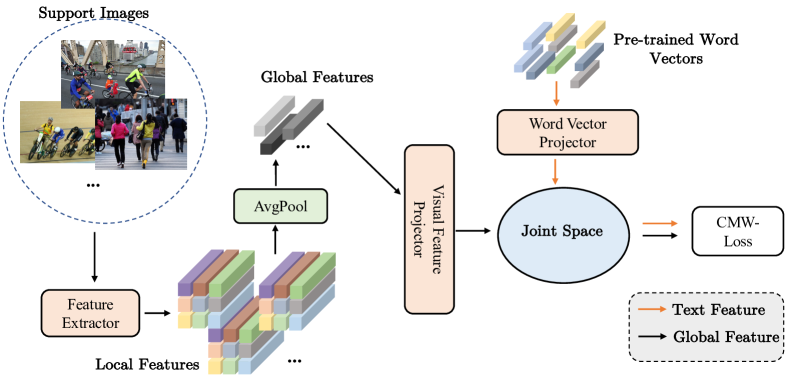
Figure 1: A joint embedding space is learned in which both labels and images are represented.

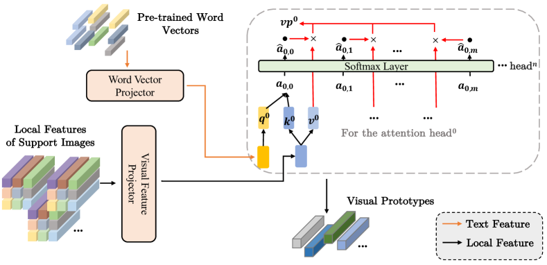
Figure 2: An attention mechanism is used to compute label prototypes from the local features of the relevant images from the support set. The embedding of the considered label plays the role of query in this attention mechanism.

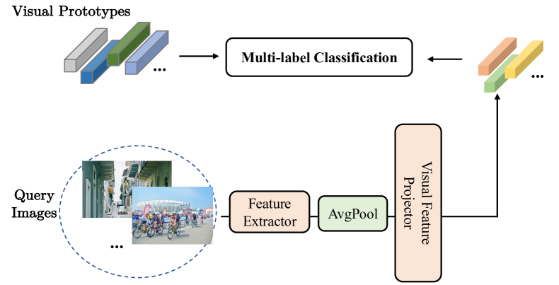
Figure 3: Query images are classified based on their distance to the visual prototypes.

4 Method

Our model consists of two main components. The first component is aimed at jointly representing label embeddings and visual features in the same vector space. Essentially, this component aims to predict visual prototypes from the label embeddings. Since such prototypes are noisy, we do not use them directly for making the final label predictions. This component is merely used to learn a joint representation of visual features and labels; it is illustrated in Figure 1. The second component is aimed at computing the final prototypes, by aggregating the local features of the corresponding support images based on an attention mechanism, which relies on the label representations that are obtained by the first component. This second component is illustrated in Figure 2. Finally, to classify a query image, we project it to the joint embedding space and then compare it with the learned prototypes, as illustrated in Figure 3. We now describe these different steps in more detail.

Joint Embedding of Visual Features and Labels

Given an input image $I$, we first use a feature extractor to obtain its local feature map $\mathbf{f}_{\textit{loc}}^{I}\in\mathbb{R}^{n\times h\times w}$, where $n$ is the number of channels, $h$ is the height and $w$ is the width. In this paper, we use a fully convolutional network such as ResNet (He et al. 2016) for this purpose. The global visual feature vector $\mathbf{f}_{\textit{glo}}^{I}$ for image $I$ is obtained by feeding the local feature map through an adaptive average pooling layer:

$$\mathbf{f}_{\textit{glo}}^{I}=\textit{AdaptiveAvgPool}(\mathbf{f}_{\textit{loc}}^{I})$$ (1)

We use pre-trained word embeddings to represent the labels in $\mathcal{C}_{\textit{base}}\cup\mathcal{C}_{\textit{novel}}$. Let us write $\mathbf{w}_{c}$ for the word vector representing label $c$, and let $d_{w}$ be the dimensionality of the word vectors. With the aim of representing images and labels in the same vector space, we learn two linear transformations:

$$\widehat{\mathbf{f}_{\textit{glo}}^{I}} =\mathbf{A}_{\textit{visual}}\,\mathbf{f}_{\textit{glo}}^{I} \widehat{\mathbf{w}_{c}} =\mathbf{A}_{\textit{text}}\,\mathbf{w}_{c}$$

where $\mathbf{A}_{\textit{visual}}\in\mathbb{R}^{d_{j}\times n}$ is used to project the global feature vector for $I$ onto a space of $d_{j}$ dimensions. Similarly, $\mathbf{A}_{\textit{text}}\in\mathbb{R}^{d_{j}\times d_{w}}$ is used to project the $d_{w}$-dimensional embedding of a label $c$ onto the same $d_{j}$-dimensional space. To ensure that the resulting image vectors $\widehat{\mathbf{f}_{\textit{glo}}^{I}}$ and label representations $\widehat{\mathbf{w}_{c}}$ are semantically compatible, we use the following loss:

$$\mathcal{L}_{\textit{cmw}} =\sum_{I\in\mathcal{S}}\sum_{i=1}^{|\mathcal{C}|}y_{i}^{I}\cdot\log\sigma(s_{i}^{I})+(1-y_{i}^{I}\cdot\log(1-\sigma(s_{i}^{I})))$$

where $\mathcal{S}$ represents the set of images from the support set of the current training episode, $\mathcal{C}=\{c_{1},...,c_{|\mathcal{C}|}\}$ is the set of labels, $\sigma(\cdot)$ is the sigmoid function and $y_{i}^{I}$ represents the ground truth, i.e. $y_{i}^{I}=1$ if image $I$ has label $c_{i}$ and $y_{i}^{I}=0$ otherwise. Finally, we have

$$s_{i}^{I}=\lambda\cos(\widehat{\mathbf{f}_{\textit{glo}}}^{I},\widehat{\mathbf{w}_{c_{i}}})$$ (2)

The scalar $\lambda$ is a hyper-parameter to address the fact that the cosine is bounded between -1 and 1. Since the aim of the loss $\mathcal{L}_{\textit{cmw}}$ is to align two different modalities (word vectors and visual features), we refer to it as the Cross-Modality Weights Loss (CMW-loss).

Constructing Attention Based Prototypes

We now explain how the label prototypes are constructed. Consider a label $c$ and suppose this label has been assigned to $m$ images from the support set. We can obtain a total of $l=h\cdot w\cdot m$ local feature vectors from these $m$ images. Let us write these local feature vectors as $\mathbf{u}_{1},...,\mathbf{u}_{l}$. We first map these feature vectors to the joint embedding space:

$$\widehat{\mathbf{u}_{i}}=\mathbf{A}_{\textit{visual}}\,\mathbf{u}_{i}$$

The prototype of $c$ will be obtained from these local feature vectors using an attention mechanism that is inspired by Vaswani et al. (2017), where the label embedding $\widehat{\mathbf{w}_{c}}$ is used as the query component. Specifically, we have

$$\mathbf{q}^{j}_{c} =\mathbf{Q}_{j}\widehat{\mathbf{w}_{c}}$$

$$\mathbf{k}^{j}_{i} =\mathbf{K}_{j}\widehat{\mathbf{u}_{i}}$$

$$\mathbf{v}^{j}_{i} =\mathbf{V}_{j}\widehat{\mathbf{u}_{i}}$$

$$(\mu^{j}_{1},...,\mu^{j}_{l}) =\textit{softmax}\left(\frac{\mathbf{q}^{j}_{c}\cdot\mathbf{k}^{j}_{1}}{\sqrt{d_{a}}},...,\frac{\mathbf{q}^{j}_{c}\cdot\mathbf{k}^{j}_{l}}{\sqrt{d_{a}}}\right)$$

$$\mathbf{p}_{c}^{j} =\sum_{i}\mu_{i}^{j}\mathbf{v}^{j}_{i}$$

where $d_{a}$ is the dimensionality of the vectors $\mathbf{q}^{j}_{c}$, $\mathbf{k}^{j}_{i}$, and $\mathbf{v}^{j}_{i}$. The vector $\mathbf{p}_{c}^{j}$ represents the contribution of the j^th attention head to the prototype of label $c$. We use a total of $n_{a}$ attention heads. The final prototype of label $c$ is given by:

$$\mathbf{p}_{c}=\textit{mlp}(\mathbf{p}_{c}^{1}\oplus...\oplus\mathbf{p}_{c}^{n_{a}})$$ (3)

where we write $\oplus$ for vector concatenation and mlp consists of two fully connected feedforward layers with GeLU activation and dropout. Since the prototype $\mathbf{p}_{c}$ should be $d_{j}$ dimensional, we have $d_{a}=\frac{d_{j}}{n_{a}}$.

To train the attention mechanism, we use the following loss function, which we refer to as the Query Loss:

$$\mathcal{L}_{\textit{query}} =\sum_{I\in\mathcal{Q}}\sum_{i=1}^{|\mathcal{C}|}y_{i}^{I}\cdot\log\sigma(q_{i}^{I})+(1-y_{i}^{I})\cdot\log(1-\sigma(q_{i}^{I}))$$

where $\mathcal{Q}$ represents the set of images from the query set of the current training episode. As before, $\mathcal{C}$ is the set of labels and $y_{i}^{I}$ represents the ground truth. The predictions $q_{i}$ are obtained as follows:

$$q_{i}^{I}=\lambda\cos(\widehat{\mathbf{f}_{\textit{glo}}}^{I},\mathbf{p}_{c_{i}})$$ (4)

with $\lambda$ the same scalar as in (2). Note that there are two key differences between $\mathcal{L}_{\textit{cmw}}$ and $\mathcal{L}_{\textit{query}}$: (i) $\mathcal{L}_{\textit{cmw}}$ is trained using the support images while $\mathcal{L}_{\textit{query}}$ is trained using the query images; and (ii) prototypes in $\mathcal{L}_{\textit{cmw}}$ are estimated from word vectors while prototypes in $\mathcal{L}_{\textit{query}}$ are those obtained by aggregating local visual features.

	Micro				Macro
	Prec	Recall	F1	AP	Prec	Recall	F1	AP
ResNet-50	9.96	17.62	12.51	11.31	10.25	17.69	13.27	19.67
ResNet-101	9.81	17.65	12.04	10.22	9.48	17.86	12.18	18.87
ViT	9.63	12.96	11.02	10.07	9.22	14.16	11.13	16.94
ResNet-50 + ViT	8.21	13.51	10.21	10.13	9.15	14.72	11.17	16.71
PLA	13.29	55.44	20.89	21.33	13.24	54.79	20.96	30.61
PLA (GloVe)	14.12	55.83	22.15	23.02	13.51	53.21	20.37	30.13
LaSO	12.31	19.77	15.09	16.83	13.64	20.03	16.11	25.41
MAML	15.42	53.21	23.11	25.42	15.63	51.63	23.82	35.30
Ours	49.72	26.60	34.21	35.30	34.50	25.07	28.91	42.84

Table 1: Experimental results for COCO.

Model Training and Evaluation

The model is trained by repeatedly sampling training episodes from $\mathcal{C}_{\textit{base}}$, as explained in Section 3. Given a training episode with support set $\mathcal{S}$ and query set $\mathcal{Q}$, the model parameters are updated using the following loss:

$$\mathcal{L}_{\textit{all}}=\mathcal{L}_{\textit{cmw}}+\gamma\mathcal{L}_{\textit{query}}$$

with $\gamma$ a hyperparameter to control the relative importance of both components. These components are defined as above, where $\mathcal{C}$ represents the the set $\mathcal{C}_{\textit{base}}$ during training.

After the model has been trained, it can be evaluated on test episodes as follows. For each episode, we first construct the prototypes using the support set, as in (3). Note that we can do this without fine-tuning any model parameters. For each query image $I$, the probability that it has label $c_{i}$ is computed as $\sigma(q_{i}^{I})$ with $q_{i}^{I}$ as defined in (4).

	Micro				Macro
	Prec	Recall	F1	AP	Prec	Recall	F1	AP
ResNet-50	14.11	39.60	20.77	16.57	12.96	39.69	21.92	27.24
ResNet-101	16.58	42.85	23.86	19.23	15.13	42.66	22.17	30.11
ViT	13.68	25.52	17.76	16.69	13.16	25.61	17.15	27.72
ResNet-50 + ViT	11.96	16.19	13.70	18.71	11.14	16.24	12.86	28.76
PLA	23.45	86.44	36.81	41.98	24.24	87.50	37.83	47.29
PLA (GloVe)	22.67	88.03	35.84	41.31	23.16	88.64	36.55	46.54
LaSO	18.71	48.48	27.02	22.12	17.11	48.12	25.20	32.50
Ours	26.78	83.97	40.19	46.28	29.64	85.44	43.35	53.26

Table 2: Experimental results for PASCAL VOC.

5 Experiments

Experimental Setup

Datasets

We have conducted experiments on two datasets. First, we used COCO (Lin et al. 2014). This dataset was already used by Alfassy et al. (2019), who proposed a split into 64 training labels and 16 test labels. However, as they did not include a validation split, we split their 64 training labels into 12 labels for validation (cow, dining table, zebra, sandwich, bear, toaster, person, laptop, bed, teddy bear, baseball bat, skis) and 52 labels for training, while keeping the same 16 labels for testing. We include images from the COCO 2014 training and validation sets. The images which do not contain any of the test and validation labels are used as the training set. Similarly, the validation set only contains images that do not contain any training or test labels. Second, we propose a new ML-FSIC dataset based on PASCAL VOC (Everingham et al. 2015), which has 20 labels. To use as many images as possible, we select the following six labels for the novel set $\mathcal{C}_{\textit{novel}}$: dog, sofa, cat, potted plant, tv monitor, sheep. The following six labels were selected for the validation split: boat, cow, train, aeroplane, bus, bird. The remaining eight labels are used for training. We use the images from the VOC 2007 training, validation and test splits, as well as the VOC 2012 training and validation splits (noting that the labels of the VOC 2012 test split are not publicly available). We again ensure that the training images do not contain any labels from the validation and test splits, and the validation images do not contain any test labels.

Methodology

Every model is trained for 200 epochs, with the first 10 epochs used as warm-up. We used the Adam optimizer with an initial learning rate of 0.001. In contrast to our model, existing methods require a fine-tuning step during the test phase. We set the number of epochs for this fine-tuning step to 40. During the test phase, we sample 200 test episodes. Different from Alfassy et al. (2019), in addition to macro-AP, we also report micro-AP. Moreover, following usual practice in ML-IC, we also report the (macro and micro) precision, recall and F1 metrics, where we assume that a label is predicted as positive if its estimated probability is greater than 0.5 (Zhu et al. 2017).

Implementation Details

We use ResNet-50 and ResNet-101 (He et al. 2016) as feature extractors. The dimensionality of the joint embedding space was set as $d_{j}=512$. When sampling episodes, we sample one image for each label to construct the support set and four images for each label to construct the query set. As word embeddings, we considered 300-dimensional GloVe (Pennington, Socher, and Manning 2014) vectors. We similarly used standard pre-trained fastText and word2vec embeddings from an online repository. Based on the validation split, for both datasets, the number of attention heads was set to 8, the 300-dimensional GloVe vectors were selected as the word embedding model, and the hyper-parameter $\gamma$ was set to 1.

Baselines

We compare with LaSO (Alfassy et al. 2019) and KGGR (Chen et al. 2020), which were designed for the ML-FSIC setting. To put the results in context, we also compare with some methods that were designed for ML-IC. First, following LaSO (Alfassy et al. 2019), we attach a standard multi-label classifier to a number of different feature extractors: ResNet-50, ResNet-101, ViT-Base (Dosovitskiy et al. 2020) and ResNet-50 + ViT-Base. We also report results for the recent state-of-the-art CNN-RNN based method PLA (Yazici et al. 2020), which to the best of our knowledge has not previously been evaluated in the ML-FSIC setting. With the exception of KGGR, we used the original source code of the different baselines to produce the results. Since we did not have access to the KGGR source code, we only compare our method against the published results from the original paper, which followed the experimental setting from LaSO. For PLA, LaSO and our method, we used ResNet-50 as the feature extractor in the main experiments. However, since the reported results of KGGR are based on ResNet-101 and GoogleNet-v3, we used the latter models as feature extractors in the comparison with KGGR.

Experimental Results

The experimental results for COCO are shown in Table 1, showing that our proposed method outperforms the other methods by a substantial margin. It is evident that large models are prone to overfitting, noting that in terms of model size, we have: ResNet-50 + ViT-Base >ViT-Base >ResNet-101 >ResNet-50. This is not unexpected given the small number of labeled examples in ML-FSIC. LaSO can improve the ResNet-50 baseline because of its data augmentation strategy. Somewhat surprisingly, PLA performs better than LaSO, which shows that its LSTM component is able to model label dependencies in a meaningful way. PLA also needs word embeddings, but in the original model these embeddings are learned from the training data itself. For comparison, we also report results for a variant where these word vectors are initialised using the 300-dimensional GloVe vectors instead; the results are shown as PLA (GloVe). As can be seen, using pre-trained word vectors does not lead to a meaningful improvement over the original PLA model. Finally, we also add results for MAML (Finn, Abbeel, and Levine 2017), which is a popular meta-learning method for FSIC, but which was not specifically designed for the ML-FSIC. To compare with KGGR, we use the 1-shot and 5-shot settings proposed by LaSO. As shown in Table 3, for ResNet-101, in the 1-shot setting we achieved a macro-AP of 55.73, compared to 52.3 for KGGR. In the 5-shot setting, we achieved a macro-AP of 68.12, compared to 63.5 for KGGR. Moreover our method can also consistently outperform both KGGR and LaSO in combination with GoogleNet-v3 (Szegedy et al. 2016). Experimental results for PASCAL VOC are shown in Table 2. We can again see that our proposed method achieves the best results.

Method	1-shot	5-shot
LaSO (GoogleNet-v3)	45.3	58.1
KGGR (GoogleNet-v3)	49.4	61.0
KGGR (ResNet-101)	52.3	63.5
Ours (GoogleNet-v3)	53.41	65.07
Ours (ResNet-101)	55.73	68.12

Table 3: Experimental results following the common data and evaluation setting from LaSO (Alfassy et al. 2019).

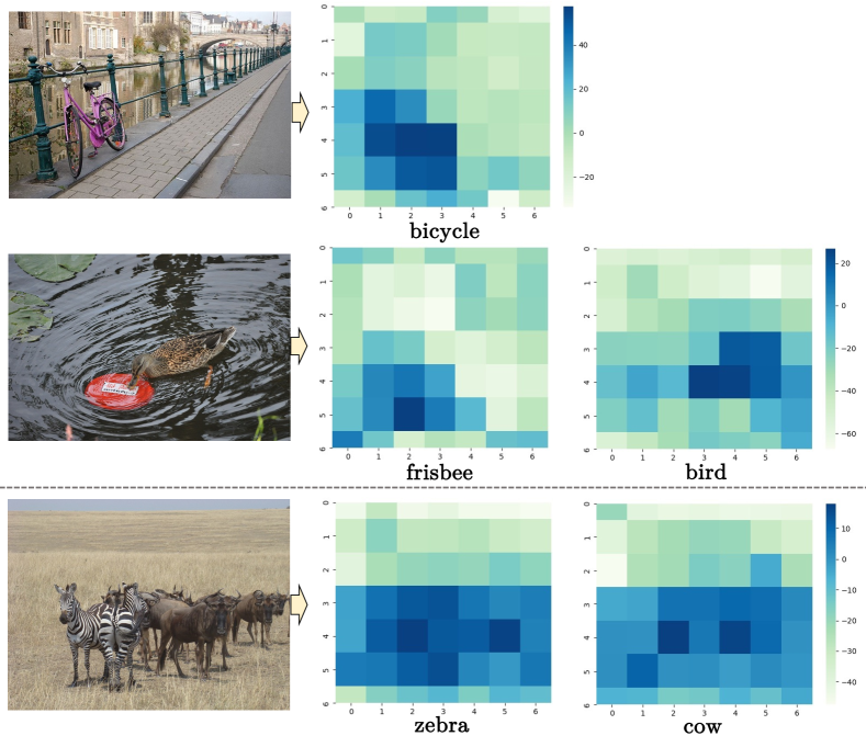
Figure 4: Visualization of the attention weights of local features for construction label prototypes. The first two examples are taken from the COCO test set, while last example is taken from the COCO validation set.

Method	Macro-AP	Micro-AP
Without CMW-loss	36.17	26.44
Simple attention	37.53	28.56
Attention with global features	35.82	27.39
Simple att. with loc. features	31.21	21.07
Low-rank bilinear pooling	33.41	24.69
Full model	42.84	35.30

Table 4: Results for different variations of the proposed model.

Word Embeddings	Macro-AP	Micro-AP
FastText	35.67	24.72
Skip-Gram	38.67	29.47
GloVe-50	27.99	17.73
GloVe-100	33.48	21.52
GloVe-200	39.13	28.86
GloVe-300	42.84	35.30
BERT	36.46	28.33

Table 5: Results for different word embeddings.

Method	Macro-AP	Micro-AP
Without Fine-tuning	42.84	35.30
With Fine-tuning	45.27	35.70

Table 6: Impact of fine-tuning during the test phase.

Ablation Study

Here we analyze the importance of the main components of our model. Some additional ablation analysis is provided in the appendix. All experiments in this section are conducted on the COCO dataset with the ResNet-50 feature extractor.

Importance of the CMW-Loss

To analyze the effect of the CMW-loss, in Table 4 we report the results that are obtained when this component of the loss function is removed. In particular, for this variant, we only use $\mathcal{L}_{\textit{query}}$ for training (using both the images from the support set and the query set in this case). Note that the alignment between the word vectors and visual features then has to be learned indirectly, together with the parameters of the overall model. As can be seen, removing the CMW-loss results in substantially lower macro-AP and micro-AP scores.

Importance of the Attention Mechanism

To evaluate the effect of the proposed attention mechanism, in Table 4 we also report results for a variant that relies on a simpler mechanism for generating prototypes (shown as Simple attention). In particular, in this variant, we generate the prototype of a label $c$ by taking a weighted average of the global features of the support images that have that label. The weights are obtained by computing the cosine similarity between the vectors $\widehat{\mathbf{w}_{c}}$ and the feature vectors $\widehat{\mathbf{f}^{I}_{\textit{glo}}}$, multiplying these cosine similarities with the scalar $\lambda$, and feeding the resulting values to a softmax layer. As shown in Table 4, in this simplified setting, there is a drop of 5.31 and 6.74 percentage points in macro-AP and micro-AP respectively. We furthermore report results of a variant where the (full) attention mechanism uses global features instead of local features (Attention with global features). We also report results when local features are used instead of global features in the simplified attention mechanism (Simplified attention with local features). Finally, we experimented with a variant that learns visual prototypes in the same way as in KGGR, where the weights of local features are generated by a low-rank bilinear pooling method followed by a fully-connected layer with softmax activation (Low-rank bilinear pooling). The results in Table 4 show that all of these variants result in lower performance.

Fine-Tuning

Although our method can be used without fine-tuning during the test phase, it is possible to fine-tune the parameters with the CMW-Loss. As shown in Table 6, fine-tuning results in an increase of 2.43 percentage points in macro-AP, but no obvious improvement in micro-AP.

Word Embeddings

Table 5 compares the results we obtained with different word embeddings: FastText (Bojanowski et al. 2017), Word2Vec (Mikolov, Yih, and Zweig 2013), GloVe (Pennington, Socher, and Manning 2014) and BERT (Devlin et al. 2019). We also experimented with GloVe vectors of 50, 100 and 200 dimensions obtained from the official GloVe project (Wikipedia 2014 + Gigaword 5). To obtain pre-trained label embeddings from BERT, we followed the setting from (Yan et al. 2021a), using BERT-base with masking. In this case, word vectors are obtained by taking the average of 1000 contextualized vectors. As can be seen in Table 5, the best results are obtained for GloVe-300.

Qualitative Analysis

Figure 4 illustrates which regions are selected by the proposed attention mechanism. For better visualization, we take the values before the softmax layer as the scores of the local features, and we take the sum of attention weights across all attention heads. As the example of the bicycle shows, the model is often successful in identifying the most relevant image region. The second example furthermore shows that the attention weights are indeed label-specific. In this example, the model correctly selects the frisbee or the duck depending on the selected label. This is despite the fact that no images with these labels were present in the training data. On the other hand, as the last example shows, for labels that are semantically closely related, such as zebra and cow in this case, word vectors are not sufficiently informative. For both labels, the model correctly selects the group of animals, but it fails to make a finer selection.

6 Conclusion

We introduced the first metric-based method for multi-label few-shot image classification. The main idea is to use word vectors to obtain noisy prototypes, which are then used to implement an attention mechanism. This attention mechanism aims to construct the final prototypes by aggregating the local features of the support images. Our model achieved substantially better results than existing models, both on COCO and a newly proposed split of PASCAL VOC. Moreover, an important advantage of our model is that it can be used without fine-tuning during the testing phase.

7 Acknowledgments

This research was supported in part by the National Key R&D Program of China (2020YFB1805400); National Natural Science Foundation of China (62072010); Capital Health Development Scientific Research Project (Grant 2020-1-4093); Clinical Medicine Plus X - Young Scholars Project, Peking University, the Fundamental Research Funds for the Central Universities; HPC resources from GENCI-IDRIS (Grant 2021-[AD011012273] and ANR CHAIRE IA BE4musIA. Shoaib Jameel is supported by NVIDIA Academic Hardware Grant;

Appendix A Additional Ablation Analysis

Number of Heads	Macro-AP	Micro-AP
1	30.06	20.39
2	35.42	27.24
4	36.68	27.02
6	35.61	27.33
8	42.84	35.30
10	42.00	34.35
12	42.70	35.96
14	40.18	35.75
16	41.53	35.66

Table 7: Impact of the number of attention heads.

Number of Attention Heads

In Table 7 we analyze the importance of using multiple attention heads. Note that when changing the number of attention heads, we keep the overall dimensionality of the prototypes fixed; e.g. when doubling the number of attention heads we halve the dimensionality of the query, key and value vectors. The results in Table 7 show that with fewer than 8 attention heads, the performance is notably lower, while there is no obvious benefit to increasing the number of attention heads beyond 8.

Scale effects

As our model uses local features with a fixed dimensionality, there is a risk that some objects are overlooked, when they are too small in the original image. To analyze this effect, we carried out a simple experiment based on ResNet-101, where we increased the image size from $224\times 224$ to $336\times 336$ and the corresponding feature map size from $2048\times 7\times 7$ to $2048\times 11\times 11$. As a result, the micro-AP and macro-AP on COCO increase from 35.30 to 36.41 and from 42.84 to 43.79 respectively. However, it should be noted that this improved performance comes at a higher computational cost.

Local Features for Query Images

In our method, we compare the global features of query images with the local features of prototypes. We also experimented with a variant in which the local features of the query image are compared with the local features of the prototypes, where the sum of the top-k values is then used as the similarity score. This variant achieves 35.59 micro-AP and 42.91 macro-AP. This represents a small improvement over our main model (35.30 micro-AP and 42.84 macro-AP), which again comes at the a significantly increased computational cost.

References

- Alfassy et al. (2019) Alfassy, A.; Karlinsky, L.; Aides, A.; Shtok, J.; Harary, S.; Feris, R.; Giryes, R.; and Bronstein, A. M. 2019. Laso: Label-set operations networks for multi-label few-shot learning. In Proceedings of the IEEE/CVF Conference on Computer Vision and Pattern Recognition, 6548–6557.
- Bojanowski et al. (2017) Bojanowski, P.; Grave, E.; Joulin, A.; and Mikolov, T. 2017. Enriching Word Vectors with Subword Information. Transactions of the Association for Computational Linguistics, 5: 135–146.
- Chen et al. (2020) Chen, T.; Lin, L.; Hui, X.; Chen, R.; and Wu, H. 2020. Knowledge-guided multi-label few-shot learning for general image recognition. IEEE Transactions on Pattern Analysis and Machine Intelligence.
- Chen et al. (2021) Chen, Z.; Ge, J.; Zhan, H.; Huang, S.; and Wang, D. 2021. Pareto Self-Supervised Training for Few-Shot Learning. In Proceedings of the IEEE/CVF Conference on Computer Vision and Pattern Recognition, 13663–13672.
- Chen et al. (2019) Chen, Z.-M.; Wei, X.-S.; Wang, P.; and Guo, Y. 2019. Multi-label image recognition with graph convolutional networks. In Proceedings of the IEEE/CVF Conference on Computer Vision and Pattern Recognition, 5177–5186.
- Devlin et al. (2019) Devlin, J.; Chang, M.; Lee, K.; and Toutanova, K. 2019. BERT: Pre-training of Deep Bidirectional Transformers for Language Understanding. In Proceedings NAACL-HLT.
- Dosovitskiy et al. (2020) Dosovitskiy, A.; Beyer, L.; Kolesnikov, A.; Weissenborn, D.; Zhai, X.; Unterthiner, T.; Dehghani, M.; Minderer, M.; Heigold, G.; Gelly, S.; et al. 2020. An image is worth 16x16 words: Transformers for image recognition at scale. arXiv preprint arXiv:2010.11929.
- Everingham et al. (2015) Everingham, M.; Eslami, S. A.; Van Gool, L.; Williams, C. K.; Winn, J.; and Zisserman, A. 2015. The pascal visual object classes challenge: A retrospective. International journal of computer vision, 111(1): 98–136.
- Finn, Abbeel, and Levine (2017) Finn, C.; Abbeel, P.; and Levine, S. 2017. Model-Agnostic Meta-Learning for Fast Adaptation of Deep Networks. In Proc. ICML, 1126–1135.
- He et al. (2016) He, K.; Zhang, X.; Ren, S.; and Sun, J. 2016. Deep residual learning for image recognition. In Proc. CVPR, 770–778.
- Kim et al. (2019) Kim, J.; Kim, T.; Kim, S.; and Yoo, C. D. 2019. Edge-labeling graph neural network for few-shot learning. In Proc. CVPR, 11–20.
- Kipf and Welling (2017) Kipf, T. N.; and Welling, M. 2017. Semi-Supervised Classification with Graph Convolutional Networks. In Proc. ICLR.
- Lanchantin et al. (2021) Lanchantin, J.; Wang, T.; Ordonez, V.; and Qi, Y. 2021. General Multi-label Image Classification with Transformers. In Proceedings of the IEEE/CVF Conference on Computer Vision and Pattern Recognition, 16478–16488.
- Li et al. (2020) Li, A.; Huang, W.; Lan, X.; Feng, J.; Li, Z.; and Wang, L. 2020. Boosting Few-Shot Learning With Adaptive Margin Loss. In Proc. CVPR, 12573–12581.
- Li et al. (2019) Li, W.; Wang, L.; Xu, J.; Huo, J.; Gao, Y.; and Luo, J. 2019. Revisiting Local Descriptor Based Image-To-Class Measure for Few-Shot Learning. In Proc. CVPR, 7260–7268.
- Li, Mozer, and Whitehill (2021) Li, Z.; Mozer, M.; and Whitehill, J. 2021. Compositional embeddings for multi-label one-shot learning. In Proceedings of the IEEE/CVF Winter Conference on Applications of Computer Vision, 296–304.
- Li et al. (2017) Li, Z.; Zhou, F.; Chen, F.; and Li, H. 2017. Meta-sgd: Learning to learn quickly for few-shot learning. arXiv preprint arXiv:1707.09835.
- Lin et al. (2014) Lin, T.-Y.; Maire, M.; Belongie, S.; Hays, J.; Perona, P.; Ramanan, D.; Dollár, P.; and Zitnick, C. L. 2014. Microsoft coco: Common objects in context. In European conference on computer vision, 740–755. Springer.
- Mikolov, Yih, and Zweig (2013) Mikolov, T.; Yih, W.-t.; and Zweig, G. 2013. Linguistic Regularities in Continuous Space Word Representations. In Proceedings NAACL-HLT, 746–751.
- Pennington, Socher, and Manning (2014) Pennington, J.; Socher, R.; and Manning, C. D. 2014. GloVe: Global Vectors for Word Representation. In Proc. EMNLP, 1532–1543.
- Ravi and Larochelle (2017) Ravi, S.; and Larochelle, H. 2017. Optimization as a Model for Few-Shot Learning. In Proc. ICLR.
- Satorras and Estrach (2018) Satorras, V. G.; and Estrach, J. B. 2018. Few-Shot Learning with Graph Neural Networks. In Proc. ICLR.
- Snell, Swersky, and Zemel (2017) Snell, J.; Swersky, K.; and Zemel, R. S. 2017. Prototypical Networks for Few-shot Learning. In Proc. NIPS, 4077–4087.
- Sung et al. (2018) Sung, F.; Yang, Y.; Zhang, L.; Xiang, T.; Torr, P. H.; and Hospedales, T. M. 2018. Learning to compare: Relation network for few-shot learning. In Proc. CVPR, 1199–1208.
- Szegedy et al. (2016) Szegedy, C.; Vanhoucke, V.; Ioffe, S.; Shlens, J.; and Wojna, Z. 2016. Rethinking the inception architecture for computer vision. In Proceedings of the IEEE conference on computer vision and pattern recognition, 2818–2826.
- Tsoumakas and Katakis (2007) Tsoumakas, G.; and Katakis, I. 2007. Multi-label classification: An overview. International Journal of Data Warehousing and Mining (IJDWM), 3(3): 1–13.
- Vaswani et al. (2017) Vaswani, A.; Shazeer, N.; Parmar, N.; Uszkoreit, J.; Jones, L.; Gomez, A. N.; Kaiser, Ł.; and Polosukhin, I. 2017. Attention is all you need. In Advances in neural information processing systems, 5998–6008.
- Wang et al. (2016) Wang, J.; Yang, Y.; Mao, J.; Huang, Z.; Huang, C.; and Xu, W. 2016. Cnn-rnn: A unified framework for multi-label image classification. In Proceedings of the IEEE conference on computer vision and pattern recognition, 2285–2294.
- Wang et al. (2020) Wang, Y.; He, D.; Li, F.; Long, X.; Zhou, Z.; Ma, J.; and Wen, S. 2020. Multi-label classification with label graph superimposing. In Proceedings of the AAAI Conference on Artificial Intelligence, volume 34, 12265–12272.
- Wang et al. (2017) Wang, Z.; Chen, T.; Li, G.; Xu, R.; and Lin, L. 2017. Multi-label image recognition by recurrently discovering attentional regions. In Proceedings of the IEEE international conference on computer vision, 464–472.
- Xing et al. (2019) Xing, C.; Rostamzadeh, N.; Oreshkin, B. N.; and Pinheiro, P. O. 2019. Adaptive Cross-Modal Few-shot Learning. In Proc. NIPS, 4848–4858.
- Yan et al. (2021a) Yan, K.; Bouraoui, Z.; Wang, P.; Jameel, S.; and Schockaert, S. 2021a. Aligning Visual Prototypes with BERT Embeddings for Few-Shot Learning. arXiv preprint arXiv:2105.10195.
- Yan et al. (2021b) Yan, K.; Bouraoui, Z.; Wang, P.; Jameel, S.; and Schockaert, S. 2021b. Few-shot image classification with multi-facet prototypes. In ICASSP 2021-2021 IEEE International Conference on Acoustics, Speech and Signal Processing (ICASSP), 1740–1744. IEEE.
- Yan et al. (2021c) Yan, K.; Liu, L.; Hou, J.; and Wang, P. 2021c. Representative Local Feature Mining for Few-Shot Learning. In ICASSP 2021-2021 IEEE International Conference on Acoustics, Speech and Signal Processing (ICASSP), 1730–1734. IEEE.
- Yazici et al. (2020) Yazici, V. O.; Gonzalez-Garcia, A.; Ramisa, A.; Twardowski, B.; and Weijer, J. v. d. 2020. Orderless recurrent models for multi-label classification. In Proceedings of the IEEE/CVF Conference on Computer Vision and Pattern Recognition, 13440–13449.
- Ye et al. (2020) Ye, H.-J.; Hu, H.; Zhan, D.-C.; and Sha, F. 2020. Few-Shot Learning via Embedding Adaptation with Set-to-Set Functions. In Proc. CVPR.
- You et al. (2020) You, R.; Guo, Z.; Cui, L.; Long, X.; Bao, Y.; and Wen, S. 2020. Cross-modality attention with semantic graph embedding for multi-label classification. In Proceedings of the AAAI Conference on Artificial Intelligence, volume 34, 12709–12716.
- Zhu et al. (2017) Zhu, F.; Li, H.; Ouyang, W.; Yu, N.; and Wang, X. 2017. Learning spatial regularization with image-level supervisions for multi-label image classification. In Proceedings of the IEEE Conference on Computer Vision and Pattern Recognition, 5513–5522.