Learning Optimal Predictive Checklists

Abstract

Checklists are simple decision aids that are often used to promote safety and reliability in clinical applications. In this paper, we present a method to learn checklists for clinical decision support. We represent predictive checklists as discrete linear classifiers with binary features and unit weights. We then learn globally optimal predictive checklists from data by solving an integer programming problem. Our method allows users to customize checklists to obey complex constraints, including constraints to enforce group fairness and to binarize real-valued features at training time. In addition, it pairs models with an optimality gap that can inform model development and determine the feasibility of learning sufficiently accurate checklists on a given dataset. We pair our method with specialized techniques that speed up its ability to train a predictive checklist that performs well and has a small optimality gap. We benchmark the performance of our method on seven clinical classification problems, and demonstrate its practical benefits by training a short-form checklist for PTSD screening. Our results show that our method can fit simple predictive checklists that perform well and that can easily be customized to obey a rich class of custom constraints.

1 Introduction

Checklists are simple tools that are widely used to assist humans when carrying out important tasks or making important decisions [13, 18, 50, 61, 64, 8, 35, 60, 44, 65, 66]. These tools are often used as predictive models in modern healthcare applications. In such settings, a checklist is a set of Boolean conditions that predicts a condition of interest – e.g., a list of symptoms flag a patient for a critical illness when $M$ out $N$ symptoms are checked. These kinds of “predictive checklists” are often used for clinical decision support because they are easy to use and easy to understand [33, 54]. In contrast to other kinds of predictive models, clinicians can easily scrutinize a checklist, and make an informed decision as to whether they will adopt it. Once they have decided to use a checklist, they can integrate the model into their clinical workflow without extensive training or technology (e.g., as a printed sheet [52]).

Considering these benefits, one of the key challenges in using predictive checklists in healthcare applications is finding a reliable way to create them [33]. Most predictive checklists in medicine are either hand-crafted by panels of experts [41, 30], or built by combining statistical techniques and heuristics [e.g., logistic regression, stepwise feature selection, and rounding 39]. These approaches make it difficult to develop checklists that are sufficiently accurate – as panel or pipeline will effectively need to specify a model that performs well under stringent assumptions on model form. Given the simplicity of the model class, it is entirely possible that some datasets may never admit a checklist that is sufficiently accurate to deploy in a clinical setting – as even checklists that are accurate at a population-level may perform poorly on a minority population [70, 57].

In this paper, we introduce a machine learning method to learn checklists from data. Our method is designed to streamline the creation of predictive checklists in a way that overcomes specific challenges of model development in modern healthcare applications. Our method solves an integer programming problem to return the most accurate checklist that obeys user-specified constraints on model form and/or model performance. This approach is computationally challenging, but provides specific functionality that simplifies and streamlines model development. First, it learns the most accurate checklist by optimizing exact measures of model performance (i.e., accuracy rather than a convex surrogate measure). Second, it seeks to improve the performance of checklists by adaptively binarizing features at training time. Third, it allows practitioners to train checklists that obey custom requirements on model form or on prediction, by allowing them to encode these requirements as constraints in the optimization problem. Finally, it provides practitioners with an optimality gap, which informs them when a sufficiently accurate checklist does not exist.

The main contributions of this paper are:

1. We present a machine learning method to learn checklists from data. Our method allows practitioners to customize models to obey a wide range of real-world constraints. In addition, it pairs checklists with an optimality gap that can inform practitioners in model development.

2. We develop specialized techniques that improve the ability of our approach to train a checklist that performs well, and to pair this model with a small optimally gap. One of these techniques can be used to train checklists heuristically.

3. We conduct a broad empirical study of predictive checklists on clinical classification datasets [51, 37, 58, 24, 32]. Our results show that predictive checklists can perform as well as state-of-the-art classifiers on some datasets, and that our method can provide practitioners with an optimality gap to flag when this is not the case. We highlight the ability of our method to handle real-world requirements through applications where we enforce group fairness constraints on a mortality prediction task, and where we build a short-form checklist to screen for PTSD.

4. We provide a Python package to train and customize predictive checklists with open-source and commercial solvers, including CBC [29] and CPLEX [20] (see https://github.com/MLforHealth/predictive_checklists).

2 Related Work

The use of checklist-style classifiers – e.g., classifiers that assign coefficients of $\pm 1$ to Boolean conditions – dates to the work of Burgess [9]. The practice is often referred to as “unit weighting," and is motivated by observations that it often performs surprisingly well [see e.g., 27, 23, 19, 7].

Our work is strongly related to methods that learn sparse linear classifiers with small integer coefficients [see e.g., 11, 31, 68, 4, 69, 38, 75]. We learn checklists from data by solving an integer program. Our problem can be viewed as a special case of an IP proposed by Ustun and Rudin [68], Zeng et al. [77] to learn sparse linear classifiers with small integer coefficients. The problem that we consider is considerably easier to solve from a computational standpoint because it restricts coefficients to binary values and does not include $\ell_{0}$-regularization. Here, we make use of this “slack" in computation to add functionality that improves the performance of checklists, namely: (1) constraints to binarize continuous and categorical features into items that can be included in a checklist [see also 10, 71, 12]; and (2) develop specialized techniques to reduce computation during the learning process.

Checklists are $M$-of-$N$ rules –- i.e., classifiers that predict $y=+1$ when $M$ out of $N$ conditions are true. Early work in machine learning used $M$-of-$N$ rules in an auxiliary capacity – e.g., to explain the predictions of neural networks [67], or to use as features in decision trees [78]. More recent work has focused on learning $M$-of-$N$ rules for standalone prediction – e.g. Chevaleyre et al. [16] describe a method to learn $M$-of-$N$ rules by rounding the coefficients of linear SVMs to $\{-1,0,1\}$ using a randomized rounding procedure [see also 79]. Methods to learn disjunctions and conjunctions are also relevant since they correspond to $1$-of-$N$ rules and $N$-of-$N$ rules, respectively. These methods learn models by solving a special case of the ERM problem in (1) where $M=1$ or $M=N$. Given that this problem is NP-hard, existing methods often reduce computation by using algorithms that return approximate solutions – e.g., simulated annealing [72], set cover [48, 49], or ERM with a convex surrogate loss [46, 21, 22, 47]. These approaches could be used to learn checklists by solving the ERM problem in (1). However, they would not be able to handle the discrete constraints needed for binarization and customization. More generally, they would not be guaranteed to recover the most accurate checklists for a given dataset, nor pair models with a certificate of optimality that can be used to inform model development.

3 Methodology

We start with a dataset of $n$ examples $(\bm{x}_{i},y_{i})_{i=1}^{n}$ where $\bm{x}_{i}=[x_{i1},\ldots,x_{id}]\in\{0,1\}^{d}$ is a vector of $d$ binary variables and $y_{i}\in\{0,1\}$ is a label. Here, $\bm{x}_{i}$ are Boolean variables that could be used as items in a checklist. We denote the indices of positive and negative examples as $I^{+}{}{}=\{i~{}|~{}y_{i}=+1\}$ and $I^{-}{}{}=\{i~{}|~{}y_{i}=-1\}$ respectively, and let $n^{+{}}{}=|I^{+}{}{}|$ and $n^{-{}}{}=|I^{-}{}{}|$. We denote the set of positive integers up to $k$ as $[{k}]=\{1,\ldots,k\}$.

We use the dataset to learn a predictive checklist – i.e., a Boolean threshold rule that predicts $\hat{y}{}=+1$ when at least $M$ of $N$ items are checked. We represent a checklist as a linear classifier with the form:

$$\hat{y}_{i}=\textrm{sign}(\bm{\lambda}^{\top}\bm{x}_{i}\geq M).$$

Here $\bm{\lambda}=[\lambda_{1},\ldots,\lambda_{d}]\in\{0,1\}^{d}$ is a coefficient vector and $\lambda_{j}=1$ iff the checklist contains item $j$. We denote the number of items in a checklist with coefficients $\bm{\lambda}$ as $N=\sum_{j=1}^{d}{\lambda_{j}}$, and denote the threshold number of items that must be checked to assign a positive prediction as $M$. We learn checklists from data by solving an empirical risk minimization problem with the form:

$$\footnotesize\begin{split}\min_{\bm{\lambda},M}\quad&l\left({\bm{\lambda},M}\right)+\epsilon_{N}N+\epsilon_{M}M\\ \textnormal{s.t.}\quad&N=\left\|\bm{\lambda}\right\|\\ \quad&M\in[{N}]\\ \quad&\bm{\lambda}\in\{0,1\}^{d}\end{split}$$ (1)

Here, $l\left({\bm{\lambda},M}\right)=\sum_{i=1}^{n}\mathds{1}\left[y_{i}\neq\hat{y}_{i}\right]$ counts the number of mistakes of a checklist with parameters $\bm{\lambda}$ and $M$. The parameters $\epsilon_{N}>0$ and $\epsilon_{M}>0$ are small penalties used to specify lexicographic preferences. We set $\epsilon_{N}<\frac{1}{nd}$ and $\epsilon_{M}<\frac{\epsilon_{N}}{d}$. These choices ensure that optimization will return the most accurate checklist, breaking ties between checklists that are equally accurate to favor smaller $N$, and breaking ties between checklists that are equally accurate and sparse to favor smaller $M$. Smaller values of $N$ and $M$ are preferable, as checklists with smaller $N$ users check fewer items, and checklists with smaller $M$ let users stop checking as soon as $M$ items are checked (see Figure 3).

We recover a globally optimal solution to (1) by solving the integer program (IP):

@c@r@ c@ l> l min_λ, z, M & l^+ + W^- l^- + ϵ_N N + ϵ_M M
s.t. B_i z_i ≥ M - ∑_j=1^d λ_j x_i, j i ∈I^+
B_i z_i ≥ ∑_j=1^d λ_j x_i, j - M +1 i ∈I^-
l^+ = ∑_i ∈I^+ z_i
l^- = ∑_i ∈I^- z_i
N = ∑_j=1^d λ_j
M ∈ [N]
z_i ∈ {0, 1} i ∈[n]
λ_j ∈{0, 1} j ∈[d]

Here, $l^{+}$ and $l^{-}$ are variables that count the number of mistakes on positive and negative examples. The values of $l^{+}$ and $l^{-}$ are computed using the mistake indicators $z_{i}=\mathds{1}\left[\hat{y}_{i}\neq y_{i}\right]$, which are set to $1$ through “Big-M" Constraints in (2) and (2).These constraints depend on the “Big-M" parameters $B_{i}$, which can be set to its tightest possible value $\max_{\lambda}{M-\lambda^{\top}\bm{x}_{i}}$. $W^{-}$ is a user-defined parameter that reflects the relative cost of misclassifying a negative example. By default, we set $W^{-}{}=1$, so that the objective minimizes training error.

Customization

The IP in (2) can be customized to fit checklists that obey a wide range of real-world requirements on performance and model form. We list examples of constraints in Table 1. Our method provides two ways of handling classification problems with different costs of False Negatives (FNs) and False Positives (FPs). First, the user can specify the relative misclassification costs for FPs and FNs in the objective function by setting $W^{-}$. Here, optimizing (2) corresponds directly to minimizing the weighted error. Second, the user can instead specify limits on FPR and FNR - e.g. minimize the training FPR (by setting $W^{-}=n^{-}$) subject to training FNR $\leq 20\%$.

Model Requirement	Example	Constraint
Model Size	Use $\leq N_{max}$ items	$N\leq N_{max}$
Procedural	If checklist includes item about coughing, then include item about fever	$\lambda_{fever}\geq\lambda_{cough}$
Prediction	Predict $\hat{y}_{i}=+1$ for all patients with both fever and coughing	$\lambda_{fever}x_{i,fever}+\lambda_{cough}x_{i,cough}\geq M\ \forall\ i\in[n]$
Class-Based Accuracy	Max FPR $\leq$ $\gamma$	$l^{-}\leq\lceil\gamma\cdot n^{-{}}{}\rceil$
Group Fairness	Max FPR disparity of $\gamma$% between males and females	$\left|\tfrac{l^{-}_{M}}{{n^{-}_{M}}}-\tfrac{l^{-}_{F}}{n^{-}_{F}}\right|\leq\gamma$
Minimax Fairness	No group with FNR worse than $\delta$	$l_{g}^{+}\leq\lceil\delta\cdot n_{g}^{+}\rceil\ \ \forall g\in G$

Table 1: Model requirements that can be addressed by our method. Each requirement can be directly encoded into IP (2). The IP can then be solved using the same MIP solver to obtain the most accurate checklist that obeys these constraints.

Adaptive Binarization

Practitioners often work with datasets that contain real-valued and categorical features. In such settings, rule-learning methods often require practitioners to binarize such features before training. Our approach allows practitioners to binarize features into items during training. This allows all items to be binarized in a way that maximizes accuracy. This approach requires practitioners to first define $T_{j}$ candidate items for each non-binary feature $u_{i,j}$. For example, given a real-valued feature $u_{i,j}\in\mathbb{R}$, the set of candidate items could take the form $\{x_{i,j,1},x_{i,j,2},\ldots,x_{i,j,T_{j}}\}$ where $x_{i,j,t}=\mathds{1}\left[u_{i,j}\geq v_{j,t}\right]$ and $v_{j,t}$ is a threshold. We would add the following constraint to IP (2) to ensure that the checklist only uses one of the $T_{j}$ items: $\sum_{t\in[{T_{j}}]}\lambda_{t_{j}}\leq 1$. In this way, the IP would then choose a binary item that is aligned with the goal of maximizing accuracy. In practice, the set of candidate items can be produced automatically [e.g., using binning or information gain 53] or specified on the basis of clinical standards (as real-valued features like blood pressure and BMI have established thresholds). This approach is general enough to allow practitioners to optimize over all possible thresholds, though this may lead to overfitting. Our experiments in Section 5.2 show that adaptive binarization produces a meaningful improvement in performance for our model class.

Optimality Gap

We solve IP (2) with a MIP solver, which finds a globally optimal solution through exhaustive search algorithms like branch-and-bound [73]. Given an instance of IP (2) and a time limit for when to stop the search, a solver returns: (i) the best feasible checklist found within the time limit – i.e., values of $\bm{\lambda}$ and $M$ that achieve the best objective value $V^{\textrm{max}}{}=l\left({\bm{\lambda},M}\right)$; and (ii) a lower bound on the objective value – i.e., $V^{\textrm{min}}{}$, the minimal objective value for any feasible solution. These quantities are used to compute the optimality gap $\varepsilon:=1-\tfrac{V^{\textrm{min}}{}}{V^{\textrm{max}}{}}.$ When the upper bound $V^{\textrm{max}}{}$ matches the lower bound $V^{\textrm{min}}{}$, the solver returns a checklist with an optimality gap of $\varepsilon=0$ – i.e., one that is certifiably optimal.

In our setting, the optimality gap reflects the worst-case difference in training error between the checklist that a solver returns and the most accurate checklist that we could hope to obtain by solving IP (2). Given a solution to IP (2) with an objective value of $L$ and an optimality gap of $\varepsilon$, any feasible checklist has a training error of at least $\lceil(1-\varepsilon)L\rceil.$ When $\varepsilon$ is small, the most accurate checklist has a training error $\approx L$. Thus, if we are not satisfied with the performance of our model, we know that no checklist can perform better than $L$, and can make an informed decision to relax constraints, fit a classifier from a more complex hypothesis class, or not fit a classifier at all. When $\varepsilon$ is large, our problem may admit a checklist with training error far smaller than $L$. If we are not satisfied with the performance of the checklist, we cannot determine whether this is because the dataset does not admit a sufficiently accurate model or because the solver has not been able to find it.

4 Algorithmic Improvements

In this section, we present specialized techniques to speed up the time required to find a feasible solution, and/or to produce a solution with a smaller optimality gap.

4.1 Submodular Heuristic

Our first technique is a submodular optimization technique that we use to generate initial feasible solutions for IP (2). We consider a knapsack cover problem. This problem can be solved to produce a checklist of $N_{\textrm{max}}$ or fewer items that: (1) maximizes coverage of positive examples; (2) has a “budget” of negative examples $B$; and (3) uses at most one item from each of the feature groups $R_{1},...,R_{T}$ where each $R_{t}$ denote a set of items derived from a particular real-valued feature and $\cup_{t=1}^{T}R_{t}=[d]$.

@c@r@ c@ l> l max_A   &    f_M^+(A)
s.t. |A| ≤ N_max
|A ∩R_t| ≤ 1 t ∈[T]
∑_j ∈A c(j) ≤ B

Here, $f_{M}^{+}:=\sum_{i\in I^{+}{}{}}\min(\sum_{j\in A}{x_{i,j}},M)$ counts the positive examples that are covered by at least $M$ items in $A$. Constraint (3) limits the number of items in the checklist. Constraint (3) requires the checklist to use at most one item from each feature group $R_{1},\ldots,R_{T}$. Constraint (3) controls the number of negative examples that are covered by at least $M$ items in $A$. This is a knapsack constraint that assigns a cost to each item as $c(j)=\sum_{i\in I^{-}{}{}}x_{i,j}$ and limits the overall cost of $A$ using the budget parameter $B>0$.

The optimization problem in (3) can be solved using a submodular minimization algorithm given that $f_{M}^{+}$ is monotone submodular (see Appendix A.1 for a proof), and that constraints (3) to (3) are special kinds of matroid constraints. We solve (3) with a submodular minimization algorithm adapted from Badanidiyuru and Vondrák [2] (Appendix A.2). The procedure takes as input $M$, $N_{max}$ and $B$ and outputs a set of checklists that use up to $N_{max}$ items. This procedure can run within 1 second. Given a problem where we would want to train a checklist that has at most $N_{\max}$ items, we would solve this problem $|\mathcal{B}|N_{\max}$ times, varying $M\in[{N_{max}}]$ and $B\in\mathcal{B}.$

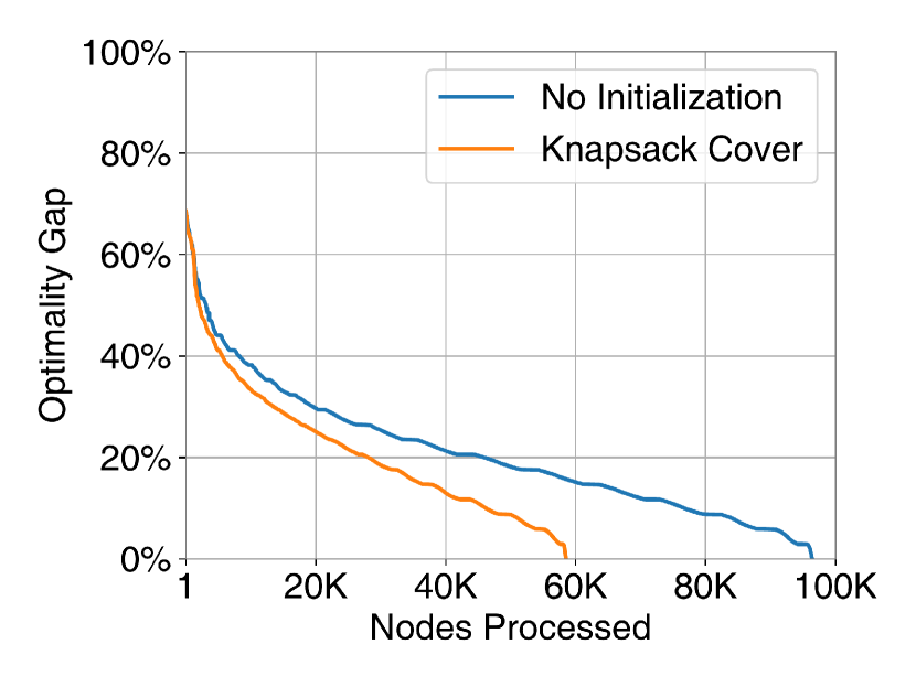
(a)

Input: maximum # of items $N_{max}$

Input: objective value function $V(\cdot)$

pool $\leftarrow\emptyset$

for $i\in[{N_{\textrm{max}}}]$, $j\in[{i}]$ do

       $S\leftarrow\{C|C\in\text{pool},N(C)\leq i,M(C)\leq j\}$

       $C_{init}\leftarrow\operatorname*{argmin}_{C\in S}f(C)$

       $C_{new}\leftarrow$ solve IP (2) with initial solution $C_{init}$ subject to $N\leq i$ and $M\leq j$

       Add $\{C_{new}\}$ to pool

end for

return pool

Algorithm 1 Sequential Training over $N$ and $M$

(b)

Figure 1: (a) Performance profile when solving IP (2) with and without initialization. We show the optimality gap vs. the # of branch-and-bound nodes when solving IP (2) for the heart dataset where $N\leq 6$ and $M\leq 2$. (b) algorithm for sequential training over $N$ and $M$.

In Figure 1a, we show the effect of initializing the IP with checklists produced using the submodular heuristic. As shown, these solutions allow us to initialize the search with a good upper bound, allowing us to ultimately recover a certifiably optimal solution faster. Our empirical results in Section 5.2 show that checklists from our submodular heuristic outperform checklists fit using existing baselines. This highlights the value of this approach as a heuristic to fit checklists (in that it can produce checklists that perform well), and as a technique for initialization (in that it can produce checklists that can be used to initialize IP (2) with a small upper bound).

4.2 Path Algorithms

Our second technique is a path algorithm for sequential training. Given an instance of the checklist IP (2), this algorithm sequentially solves smaller instances of IP (2). The algorithm exploits the fact that small instances can be solved to optimality quickly and thus “ruled out" of the feasible region of subsequent instances. The resulting approach can reduce the size of the branch-and-bound tree and improve the ability to recover a checklist with a small optimality gap. These algorithms can wrap around any procedure to solve IP (2).

In Algorithm 1, we present a path algorithm to train checklists over the full range of model sizes from $1$ to $N^{\textrm{max}}$. The algorithm recovers a solution to a problem with a hard model size limit by solving smaller instances with progressively larger limits of $N_{\textrm{max}}$ and $M_{\textrm{max}}$. We store the best feasible solution from each iteration in a pool, which is then used to initialize future iterations. If the best feasible solution is certifiably optimal, we add a constraint to constrict the search space for subsequent instances. This allows us to reduce the size of the branch-and-bound tree, resulting in a faster solution in each iteration.

5 Experimental Results

In this section, we benchmark the performance of our methods on seven clinical prediction tasks.

5.1 Setup

Dataset	$d_{T}$	$d_{pct}$	$n$	Prediction Task	Reference
adhd	5	20	594	Patient diagnosed with ADHD	[51]
cardio	40	52	8,815	Patient with cardiogenic shock died in hospital	[58]
kidney	17	80	1,722	Patient with kidney failure died after renal replacement therapy	[37]
mortality	50	484	21,139	Patient died in hospital	[37]
ptsd	20	80	873	Patient has a PCL-5 PTSD diagnosis	[51]
readmit	42	94	9,766	Patient re-admitted to hospital within 30 days	[32]
heart	13	82	303	Patient has heart disease	[24]

Table 2: Clinical prediction tasks used in Section 5. Here, $n$ is the number of samples prior to oversampling, $d_{T}$ is the number of feature groups, and $d_{pct}$ is the number of features after binarization using the adaptive method.

Data.

We consider seven clinical classification tasks shown in Table 2. For each task, we create a classification dataset by using each of the following techniques to binarize features:

• Fixed: We convert continuous and ordinal features into threshold indicator variables using the median, and convert categorical feature into an indicator for the most common category.

• Adaptive: We convert continuous and ordinal features into 4 threshold indicator variables using quintiles as thresholds, and convert each categorical feature with a one-hot encoding.

• Optbinning: We use the method proposed by Navas-Palencia [53] to binarize all features.

We process each dataset to oversample the minority class to equalize the number of positive and negative examples due to class imbalance.

Methods.

We compare the performance of the following methods for creating checklists:

• MIP: We fit a predictive checklist by solving an instance of IP (2) with the appropriate constraints. We solve this problem using CPLEX 12.10 [20] paired with the computational improvements in Section 4 on a 2.4 GHz CPU with 16 GB RAM for $\leq 60$ minutes.

• Cover: We fit a predictive checklist using the submodular heuristic in Section 4.1. We set $N_{max}=8$, and vary $M\in[{N_{max}}]$ and $B\in\{kn^{+}|k\in\{\tfrac{1}{3},\frac{1}{2},1,2,3\}\}$.

• Unit: We fit a predictive checklist using unit weighting [7]. We fit $L_{1}$-regularized logistic regression models for $L_{1}$ penalties $\in[10^{-5},10]$. We convert each model into an array of checklists by including items with positive coefficients and the complements of items with negative coefficients. We convert each logistic regression model into multiple checklists by setting $M\in[{N}]$.

Evaluation.

We use 5-fold cross validation and report the mean, minimum, and maximum test error across the five folds. We use the training set of each fold to fit a predictive checklist that contains at most $N\leq 8$ items, and that is required to select at most 1 item from a feature group. We report the training error of a final model trained on all available data.

We report results for MIP checklists where $M=1$, which we refer to as MIP_OR since it corresponds to an OR rule. Finally, we report performance for $L_{1}$-regularized logistic regression (LR) and XGBoost (XGB) as baselines to evaluate performance. We train these methods using all features in an adaptive-binarized dataset to produce informal “lower bounds” on the error rate.

For each method and each dataset, we report the performance of models that achieve the lowest training error with $N\leq 8$ items. We compare the performance of Fixed and Adaptive binarization here, and report performance of Optbinning in Appendix D.2.

5.2 Results

In Table 3, we report performance for each method on each dataset when using Fixed binarization and Adaptive binarization. We report the corresponding results for Optbinning in Appendix D.2 due to space limitations. In Figure 3, we show the performance effects of varying $N$. Lastly, we show predictive checklists trained using our method in Figure 3 and Appendix D.3. In what follows, we discuss these results.

Fixed Binarization Adaptive Binarization Lower Bounds Dataset Metric Unit Cover MIP_OR MIP Unit Cover MIP_OR MIP LR XGB adhd $n={632}$ $d_{pct}={20}$ test error (%) (min, max) train error (%) gap (%) 16.0 (11.9, 19.0) 11.4 - 17.1 (13.5, 20.6) 11.1 - 16.0 (11.9, 19.0) 11.4 0.0 17.1 (13.5, 20.6) 11.1 0.0 1.4 (0.8, 2.4) 1.1 - 6.3 (2.4, 11.7) 5.4 - 5.2 (4.0, 7.9) 5.4 0.0 0.5 (0.0, 0.8) 0.5 0.0 1.1 (0.8, 2.4) 0.5 - 1.6 (0.8, 2.4) 1.1 - cardio $n={15254}$ $d_{pct}={51}$ test error (%) (min, max) train error (%) gap (%) 23.8 (21.1, 26.5) 25.0 - 25.3 (21.4, 27.2) 26.2 - 29.6 (28.4, 31.0) 29.6 19.5 24.1 (22.5, 25.6) 24.1 82.8 23.0 (21.7, 24.9) 23.0 - 25.3 (23.7, 26.8) 25.5 - 29.2 (27.7, 30.9) 29.2 51.9 22.6 (21.5, 24.1) 22.5 83.2 21.6 (20.2, 23.3) 20.6 - 26.3 (25.0, 27.7) 6.4 - kidney $n={1760}$ $d_{pct}={80}$ test error (%) (min, max) train error (%) gap (%) 33.2 (33.2, 33.2) 32.4 - 35.6 (31.8, 38.9) 33.6 - 37.2 (34.7, 40.6) 36.7 45.7 33.3 (31.2, 36.1) 31.0 78.9 37.9 (36.1, 39.8) 34.1 - 37.2 (36.4, 38.6) 36.5 - 34.7 (33.2, 36.9) 34.0 43.3 33.8 (31.2, 37.5) 30.4 82.4 30.9 (28.7, 33.5) 27.2 - 25.3 (20.2, 28.7) 0.2 - mortality $n={36684}$ $d_{pct}={478}$ test error (%) (min, max) train error (%) gap (%) 34.3 (33.1, 36.1) 32.9 - 38.1 (37.4, 39.7) 36.9 - 37.2 (36.6, 38.4) 37.4 0.0 29.1 (27.8, 30.2) 29.0 81.0 33.8 (32.3, 35.5) 33.4 - 36.5 (35.5, 37.0) 36.5 - 37.8 (37.0, 39.4) 37.8 34.0 29.2 (29.0, 29.5) 29.6 80.4 25.0 (23.5, 26.4) 22.6 - 28.0 (27.2, 29.1) 4.6 - ptsd $n={1106}$ $d_{pct}={80}$ test error (%) (min, max) train error (%) gap (%) 10.9 (7.7, 14.9) 8.3 - 10.3 (9.1, 12.6) 9.5 - 13.8 (12.2, 15.8) 13.4 0.0 11.0 (6.8, 14.9) 8.2 0.0 10.2 (7.7, 12.7) 9.2 - 12.6 (7.7, 20.3) 10.8 - 16.2 (16.2, 16.2) 12.5 0.0 8.7 (5.9, 11.7) 5.6 66.5 8.0 (5.9, 10.4) 2.8 - 4.6 (1.8, 6.4) 0.0 - readmit $n={16732}$ $d_{pct}={90}$ test error (%) (min, max) train error (%) gap (%) 35.3 (33.8, 37.2) 35.2 - 37.5 (35.3, 40.0) 37.3 - 37.9 (36.4, 39.3) 36.5 49.3 36.2 (33.8, 37.1) 35.2 81.0 34.2 (32.6, 35.5) 34.4 - 34.6 (32.6, 36.2) 34.4 - 35.2 (34.8, 35.5) 33.2 49.9 33.9 (32.6, 35.7) 33.1 73.4 33.0 (32.2, 33.8) 32.0 - 36.6 (34.7, 38.1) 13.9 - heart $n={330}$ $d_{pct}={82}$ test error (%) (min, max) train error (%) gap (%) 16.3 (13.6, 24.2) 15.2 - 18.5 (12.1, 25.8) 16.4 - 29.1 (21.2, 39.4) 23.6 0.0 28.8 (28.8, 28.8) 13.9 0.0 16.1 (7.6, 31.8) 15.2 - 23.9 (15.2, 33.3) 18.2 - 29.1 (21.2, 39.4) 23.6 0.0 16.7 (13.6, 19.7) 13.6 54.5 17.6 (10.6, 27.3) 15.2 - 17.6 (12.1, 25.8) 9.7 -

Table 3: Performance results of all methods on all datasets. For checklist models, we report the training error, test error, and optimality gap for the checklist that minimizes training error and satisfies all constraints. The intervals under test error reflect the 5-CV minimum and maximum test error. We additionally report results for LR and XGB as performance baselines that represent an informal lower bound on the error of possible checklists.

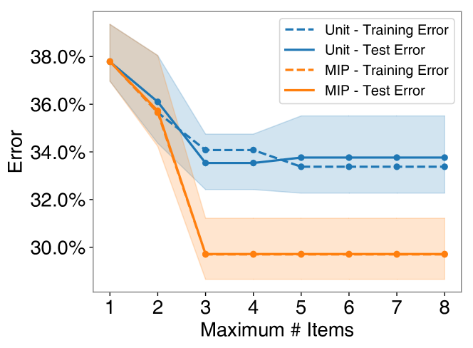
Figure 2: Performance of checklists with $\leq N$ items on mortality fit using our approach and unit weighting.

Predict 30-day readmission if 3+ items are checked # admissions past year $\geq$ 1 $\square$ bed days $\geq$ 14 $\square$ length of stay $\geq$ 8 days $\square$ chronic or uncontrolled pain $\square$ mood problems past 5 years $\square$ substance abuse past month $\square$

Figure 3: Predictive checklist fit for readmit using MIP. The checklist has a train error of 33.1%, and a test error of 33.9%. We show sample checklists for all other datasets in Appendix D.3.

On Performance

Our results in Table 3 show that our method MIP outperforms existing techniques to fit checklists (Unit) on 7/7 datasets in terms of training error, and on 5/7 datasets in terms of 5-fold CV test error. As shown in Figure 3, this improvement typically holds across all values of $N$.

In general, we find that relaxing the value of $M$ yield performance gains across all datasets (see e.g., results for ptsd where the difference in test error between MIP_OR and MIP is 7.8%), though smaller values of $M$ can produce checklists that are easier to use (see checklists in Appendix D.3).

The results in Table 3 also highlight the potential of adaptive binarization to improve performance by binarizing during training time, as MIP with adaptive binarization achieves a better training error than fixed binarization for 6/7 datasets and a better test error on 5/7 datasets.

The performance loss of checklists relative to more complex model classes (LR and XGB) varies greatly between datasets. Checklists trained on heart and readmit perform nearly as well as more complex classifiers. On mortality and kidney, however, the loss may exceed 5%.

On Generalization

Our results show that checklist performance on the training set tends to generalize well to the test set. This holds for checklists trained using all methods (i.e., Unit, Cover, MIP_OR, and MIP), which is expected given that checklists belong to a simple model class. Generalization can help us customize checklists in an informed way as we can assume that any changes to the training loss (e.g. with the addition of a constraint) lead to similar changes in the test set. In this regime, practitioners can evaluate the impact of model requirements on predictive performance – since they can measure differences in training error between checklists that obey different requirements, and expect these differences in training error as a reliable proxy for differences in test error.

On the Value of an Optimality Gap

One of the benefits of our approach is that it pairs each checklist with an optimality gap, which can inform model development by identifying settings where we cannot train a checklist that is sufficiently accurate (see Section 3). On heart, we train a checklist with a training error of 13.6% and an optimality gap of 54.5%, which suggests that there may exist a checklist with a training error of 6.2%. This optimality gap is not available for checklists trained with a heuristic (like unit weighting or domain expertise), so we would not be able to attribute poor model performance to a difficult problem, or to the heuristic being ineffective.

On Fairness

We analyze the fairness of MIP checklists trained on the kidney dataset. The task is to predict in-hospital mortality for ICU patients with kidney failure after receiving Continuous Renal Replacement Therapy (CRRT). In this setting, a false negative is often worse than a false positive, so we train checklists that minimize training FPR under a constraint to limit training FNR to 20%, using an 80%/20% train/test split.

We find that our checklist exhibit performance disparities across sex and race, which is consistent with the tendency of simpler models to exhibit performance disparities [40]. To address this issue, we train a new checklist by solving a version of IP (2) with constraints that limit disparities in training FPR and FNR over 6 intersectional groups $g\in G={\footnotesize\{\texttt{Male},\texttt{Female}\}\times\{\texttt{White},\texttt{Black},\texttt{Other}\}}$. Specifically, 30 constraints that limit the FPR disparity across groups to 15%, and 6 constraints to cap the max FNR for each intersectional group to 20%. This is unique compared to prior methods in fair classification work [76] because it enforces group fairness using exact measures[i.e., without convex relaxations 45] and over intersectional groups .

We find that we can limit performance disparities across all values of $N$ (see Figures 4 and 5, and Appendix D.4), observing that MIP with group fairness constraints has larger FPR overall but exhibits lower FPR disparities over groups (e.g., reducing the test set FPR gap between Black Females and White Males from 54.5% to 30.6%).

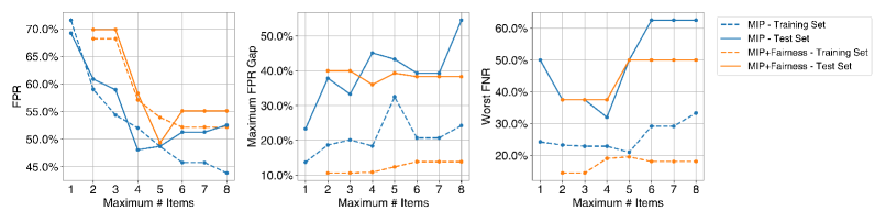
Figure 4: FPR (left), maximum FPR disparity (center) and worst-case FNR (right) versus number of items for checklists for mortality prediction given CRRT using kidney. Group fairness constraints effectively limit the FPR disparity and worst-case FNR during training, at the cost of overall performance.

Predict Mortality Given CRRT if 3+ Items are Checked Age $\geq$ 66.0 years $\square$ AST $\geq$ 162.6 IU/L $\square$ Blood pH $\leq$ 7.29 $\square$ MCV $\geq$ 99.0 fl $\square$ Norepinephrine $\geq$ 0.1 mcg/kg/min $\square$ Platelets $\leq$ 65.0 $\times 10^{3}/\mu L$ $\square$ RDW $\geq$ 19.2% $\square$ Time in ICU $\geq$ 14.1 hours $\square$	Predict Mortality Given CRRT if 2+ Items are Checked ALT $\geq$ 16.0 IU/L $\square$ Bicarbonate $\leq$ 17.0 mmol/L $\square$ Blood pH $\leq$ 7.22 $\square$ Norepinephrine $\geq$ 0.1 mcg/kg/min $\square$ RDW $\geq$ 19.2% $\square$ Time in ICU $\geq$ 117.3 hours $\square$
FNR FPR Worst FNR Max FPR Gap Training 20.0% 43.9% 33.3% 24.3% Test 22.2% 52.6% 62.5% 54.5%	FNR FPR Worst FNR Max FPR Gap Training 17.5% 52.2% 18.1% 13.9% Test 19.6% 55.1% 50.0% 38.3%
(a) MIP	(b) MIP + Fairness Constraints

Figure 5: Checklists trained to predict mortality given CRRT (a) without group fairness constraints and (b) with group fairness constraints. Checklist (a) has better overall FPR, but has worse FNR for the worst-case group, and exhibits disparities in FPR across groups. Checklist (b) obeys group fairness constraints that attenuate the training FPR gap to 15% and the worst-case FNR to 20%.

6 Learning a Short-Form Checklist for PTSD Screening

In this section, we demonstrate the practical benefits of our approach by learning a short-form checklist for Post-Traumatic Stress Disorder (PTSD) diagnosis.

Background

The PTSD Checklist for DSM-5 (PCL-5) is a self-report screening tool for PTSD [5, 74]. The PCL-5 consists of 20 questions that assess the severity of symptoms of PTSD DSM-5. Patients respond to each question with answers of Not at all, A little bit, Moderately, Quite a bit, or Extremely. Given these responses, the PCL assigns a provisional diagnosis of PTSD by counting the number of responses of Moderately or more frequent across four clusters of questions. Patients with a provisional diagnosis are then assessed for PTSD by a specialist. The PCL-5 can take over 10 minutes to complete, which limits its use in studies that include the PCL-5 in a battery of tests (i.e., using the provisional diagnosis to evaluate the prevalence of PTSD and its effect as a potential confounder), and has led to the development of short-form models [see e.g., 6, 43, 80].

Problem Formulation

Our goal is to create a short-form version of the PCL-5 – i.e., a checklist that assigns the same provisional diagnoses as PCL-5 using only a subset of the 20 questions. We train our model using data from the AURORA study [51], which contains PCL-5 responses of U.S. patients who have visited the emergency department following a traumatic event. Here, $y_{i}=+1$ if the patient is assigned a provisional PTSD diagnosis. We encode the response for each question into four binary variables $x_{i,k,l}=\mathds{1}\left[q_{k}\geq l\right]$ where $q_{k}$ is the response to each question and $l\in[{4}]$ is denotes its response. Our final dataset contains $d=80$ binary variables for $n=873$ patients, which we split into an 80% training set and 20% test set.

Since this checklist would be used to screen patients, a false negative diagnosis is less desirable than a false positive diagnosis. We train a checklist that minimizes FPR and that obeys the following operational constraints: (1) limit FNR to 5%; (2) pick one threshold for each PCL-5 question; (3) use at most 8 questions. We make use of the same methods and techniques as in Section 5.2.

Results

Our results show that short-form checklists fit using our method outperform other checklists (see Figure 7). In Figure 7, we display a sample $N=8,M=4$ checklist trained with our method which reproduces the PCL-5 diagnosis with high accuracy, offering an alternative to the PCL-5 with simpler binary items and less than half the number of questions.

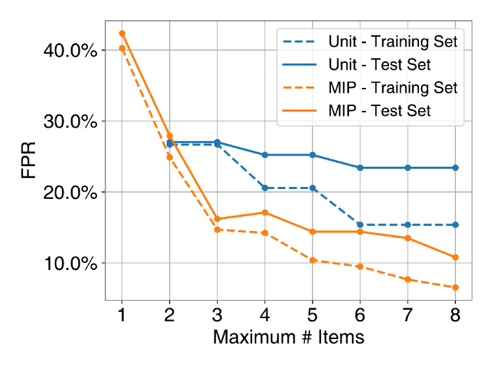
Figure 6: FPR versus number of items for short-forms of the PCL-5. MIP outperforms Unit across all values of $N$.

Predict PTSD if 4+ Items are Checked Avoiding thinking about experience $\geq$ moderately $\square$ Avoiding activities or situations $\geq$ moderately $\square$ Blame for stressful experience $\geq$ a little bit $\square$ Feeling distant or cut off $\geq$ quite a bit $\square$ Irritable or angry outbursts $\geq$ moderately $\square$ Loss of interest in activities $\geq$ moderately $\square$ Repeated disturbing dreams $\geq$ moderately $\square$ Trouble experiencing positive feelings $\geq$ moderately $\square$

Figure 7: Short-form of the PCL-5 trained with MIP. The checklist has a train/test FPR of 6.6%/10.8%, and a train/test FNR of 4.7%/6.3%. It reproduces the PCL-5 diagnosis on the training/test sets with 94.1/90.9% accuracy, and has a 70.8% optimality gap. We show condensed PCL-5 questions due to space constraint.

7 Concluding Remarks

In this work, we presented a machine learning method to learn predictive checklists from data by solving an integer program. Our method illustrates a promising approach to build models that obey constraints on qualities like safety [1] and fairness [3, 14]. Using our approach, practitioners can potentially co-design checklists alongside clinicians – by encoding their exact requirements into the optimization problem and evaluating their effects on predictive performance [17, 36].

We caution against the use of items in a checklist as causal factors of outcomes (i.e., questions in the short-form PCL are not “drivers” of PTSD), and against the use of our method solely due to its interpretability. Recent work has argued against the use of models simply because they are “interpretable" [25] and highlights the importance of validating claims on interpretability through user studies [42, 59].

We emphasize that effective deployment of the checklist models we create does not end at adoption. The proper integration of our models in a clinical setting will require careful negotiation at the personal and institutional level, and should be considered in the context of care delivery [28, 63, 62] and clinical workflows [55, 26].

Appendix A Submodular Optimization Algorithms

A.1 Proof of Monotonicity and Submodularity

In Equation (3), we stated the objective of the knapsack cover to be

$$f_{M}^{+}(A)=\sum_{i\in I^{+}{}{}}\min\left(\sum_{j\in A}{x_{i,j}},M\right)$$

defined over a ground set $\Omega$. Here, we prove that it is monotone submodular.

Remark 1.

$f_{M}^{+}$ is monotonically increasing.

Proof.

Let $e\in\Omega$ and $A^{\prime}:=A\cup\{e\}$. Since $x_{i,j}\in\{0,1\}$, $\displaystyle\sum_{j\in A^{\prime}}{x_{i,j}}\geq\displaystyle\sum_{j\in A}{x_{i,j}}\ \forall\ i\in I^{+}{}$, and thus $f_{M}^{+}(A^{\prime})\geq f_{M}^{+}(A)$. ∎

Remark 2.

$f_{M}^{+}$ is submodular. i.e.

$$\forall A\subseteq B\subseteq\Omega,\ \forall e\in\Omega,\ f_{M}^{+}(B\cup\{e\})-f_{M}^{+}(B)\leq f_{M}^{+}(A\cup\{e\})-f_{M}^{+}(A)$$

Proof.

$$\ f_{M}^{+}(B\cup\{e\})-f_{M}^{+}(B)$$

$$= \sum_{i\in I^{+}{}{}}\min\left(\sum_{j\in B\cup\{e\}}{x_{i,j}},M\right)-\min\left(\sum_{j\in B}{x_{i,j}},M\right)$$

$$= \sum_{i\in I^{+}{}{}}x_{i,e}\mathbb{I}\left(\sum_{j\in B}x_{i,j}<M\right) \text{Since }x_{i,e},x_{i,j}\in\{0,1\}\text{ and }M\in\mathbb{N}$$

$$\leq \sum_{i\in I^{+}{}{}}x_{i,e}\mathbb{I}\left(\sum_{j\in A}x_{i,j}<M\right) \text{Since }A\subseteq B\text{ and }x_{i,j}\in\{0,1\}$$

$$= f_{M}^{+}(A\cup\{e\})-f_{M}^{+}(A)$$

A.2 Knapsack Cover

To find a solution to problem 3, we use the greedy algorithm proposed by Badanidiyuru and Vondrák [2], which deals with submodular maximization subject to a system of $l$ knapsack constraints and with $p$ matroid constraints. We present an adapted version of the algorithm in Algorithm 2 where $l=1$. Here, $p=2$ if both the maximum item constraint (i.e. cardinality matroid) and the one item per feature group constraint (i.e. partition matroid) are enforced. The $\epsilon$ parameter allows us to trade-off solution time and solution quality. In this work, we set $\epsilon=0.2$. This algorithm yields a $1/(p+3+\epsilon)$ approximation ratio [2].

Input: feature set $A$, submodular function $f:2^{A}\rightarrow\mathbb{R}_{+}$, oracle for $p$-system $\mathcal{I}$, budget $B\in\mathbb{R}_{+}$, cost function $c:A\rightarrow[0,B]$, step size $\epsilon>0$

Output: A set of possible solutions $\mathcal{S}$, with each solution $S\in\mathcal{S}$, $S\subseteq A$, satisfying $S\in\mathcal{I}$ and $\sum_{j\in S}c(j)\leq B$

1

2$n\leftarrow|A|$

3 $m\leftarrow\max_{j\in A}f(j)$

4 $\mathcal{S}\leftarrow\emptyset$

5 for $\rho\leftarrow\frac{m}{p+1},(1+\epsilon)\frac{m}{p+1},...,\frac{2nm}{p+1}$ do

6       $\tau\leftarrow\max\{f(j):\frac{f(j)}{c(j)/B}\geq\rho\}$

7       $S\leftarrow\emptyset$

8       while $\tau\geq\frac{\epsilon m}{n}$ and $\sum_{j\in S}c(j)\leq B$ do

9             for $j\in A$ do

10                   $\delta\leftarrow f(S\cup\{j\})-f(S)$

11                   if $S\cup\{j\}\in\mathcal{I}$ and $\delta\geq\tau$ and $\frac{\delta}{\sum_{j\in S}{c_{j}/B}}\geq\rho$ then

12                         $S\leftarrow S\cup\{j\}$

13                         if $\sum_{j\in S}c(j)>B$ then

14                               $\mathcal{S}\leftarrow\mathcal{S}\cup(S\setminus\{j\})$

15                               $\mathcal{S}\leftarrow\mathcal{S}\cup\{j\}$

16                               goto 2

17                              

18                         end if

19                        

20                   end if

21                  

22             end for

23            $\tau\leftarrow\frac{1}{1+\epsilon}\tau$

24       end while

25      

26 end for

return $\mathcal{S}$

Algorithm 2 Greedy Knapsack Cover (one knapsack constraint and $p$ matroid constraints).

Appendix B Sequential Training Algorithms

Error Path

To learn optimal checklists for a problem subject to $FNR\leq FNR_{max}$ while minimizing FPR, we can sequentially train checklists with an increasingly larger $FNR$ constraint, using all previously trained checklists as initial solutions. This allows us to obtain an array of checklists across the ROC curve. We present this algorithm in Algorithm 3.

Input: $FNR_{max}$, grid width $\epsilon$, loss function $f$

pool $\leftarrow\emptyset$

for $i\leftarrow\epsilon,2\epsilon,...,FNR_{max}$ do

       $S\leftarrow\{C|C\in\text{pool},FNR(C)\leq i\}$

       $C_{init}\leftarrow\operatorname*{argmin}_{C\in S}f(C)$

       $C_{new}\leftarrow$ solve Formulation (2) with initial solution $C_{init}$ subject to $N\leq i$, potentially with Algorithm 1

       pool $\leftarrow$ pool $\cup\{C_{new}\}$

end for

return pool

Algorithm 3 Sequential Training with $FNR$ constraint

Appendix C Hyperparameter Grid for Baselines

Here, we describe the hyperparameter grids for the lower bound baselines shown in Table 3. For LR, we use L1 regularized logistic regression from the Scikit-Learn library [56], using the liblinear optimizer and varying $C\in\{10^{-4},10^{-3.5},...,10^{1}\}$. For XGB, we use the XGBoost library [15], varying the maximum depth $\in\{1,2,...,6\}$ and setting all other hyperparameters at default values.

Appendix D Supporting Material for Experimental Results

D.1 Datasets

All datasets used in this paper (i.e. in Table 2) are publicly available, with the exception of readmit. Datasets based on MIMIC-III [37] (kidney, mortality) and eICU [58] (cardio) are hosted on PhysioNet under the PhysioNet Credentialed Health Data License. The ADHD and PTSD datasets are from the AURORA study [51], which is hosted on the National Institute of Mental Health (NIMH) data archive, subject to the NIMH Data Use Agreement. The heart dataset is hosted on the UCI Machine Learning Repository under an Open Data license. In cases where data access requires consent or approval from the data holders, we have followed the proper procedure to obtain such consent. All datasets used in this study have been deidentified and contain no offensive content. We briefly describe each dataset and preprocessing steps taken below.

adhd

We use data from the attention deficit hyperactivity disorder (ADHD) questionnaire contained within the AURORA study [51], which consists of of U.S. patients who have visited the emergency department (ED) following a traumatic event. It consists of five questions selected from the Adult ADHD Self-Report Scale (ASRS-V1.1) Symptom Checklist (specifically, questions 1, 9, 12, 14, and 16), answered on a 0-4 ordinal scale (i.e. 0 = never, 1 = rarely, 2 = sometimes, 3 = often, 4 = very often). The target is the patient’s clinical ADHD status. This results in a dataset containing 594 patients with a prevalence of 46.8%.

cardio

Cardiogenic shock is a serious acute condition where the heart cannot provide sufficient blood to the vital organs. Using the eICU Collaborative Research Database V2.0 [58], we create a cohort of patients who have cardiogenic shock during the course of their intensive care unit (ICU) stay using an exhaustive set of clinical criteria based on the patient’s labs and vitals (i.e. presence of hypotension and organ hypoperfusion). The goal is to predict whether a patient with cardiogenic shock will die in hospital. As features, we summarize (minimums and maximums) relevant labs and vitals (e.g. systolic BP, heart rate, hemoglobin count) of each patient from the period of time prior to the onset of cardiogenic shock up to 24 hours. This results in a dataset containing 8,815 patients, 13.5% of whom die in hospital.

kidney

Using MIMIC-III and MIMIC-IV [37], we create a cohort of patients who were given Continuous Renal Replacement Therapy (CRRT) at any point during their ICU stay. For patients with multiple ICU stays, we select their first one. We define the target as whether the patient dies during the course of their selected hospital admission. As features, we select the most recent instances of relevant lab measurements (e.g. sodium, potassium, creatinine) prior to the CRRT start time, along with the patient’s age, the number of hours they have been in ICU when CRRT was administered, and their Sequential Organ Failure Assessment (SOFA) score at admission. We treat all variables as continuous with the exception of the SOFA score, which we treat as ordinal. This results in a dataset of 1,722 CRRT patients, 51.1% of which die in-hospital. We define protected groups based on the patient’s sex and self-reported race and ethnicity.

mortality

We follow the cohort creation steps outlined by Harutyunyan et al. [34] for their in-hospital mortality prediction task. We select the first ICU stay longer than 48 hours of patients in MIMIC-III [37], and aim to predict whether they will die in-hospital during their corresponding hospital admission. As features, we bin the time-series lab and vital measurements provided by Harutyunyan et al. [34] into four 12-hour time-bins, and compute the mean in each time-bin. We additionally include the patient’s age and sex as features. This results in a cohort of 21,139 patients, 13.2% of whom die in hospital.

ptsd

We use data from the PTSD questionnaire contained within the AURORA study [51], which consists of U.S. patients who have visited the emergency department following a traumatic event. It consists of responses to all items on the PTSD Checklist for DSM-5 (PCL-5), which are answered on a 0-4 ordinal scale (i.e. 0 = not at all, 1 = a little bit, 2 = moderately, 3 = quite a bit, 4 = extremely). To obtain the PCL-5 diagnosis, we use the DSM-5 diagnostic rule [5], which assigns a positive diagnosis to those with a moderately or higher on at least: 1 Criterion B item (questions 1-5), 1 Criterion C item (questions 6-7), 2 Criterion D items (questions 8-14), 2 Criterion E items (questions 15-20). This results in a dataset containing 873 patients with a prevalence of 36.7%.

heart

We use the Heart dataset from the UCI Machine Learning Repository, where the goal is to predict the presence of heart disease from clinical features. It consists of 303 patients, 54.5% of which have heart disease. We use all available features, treating cp, thal, ca, slope and restecg as categorical, and all remaining features as continuous.

readmit

The readmit dataset involves predicting 30-day hospital readmission using features derived from natural language processing on clinical records at the Massachusetts General Hospital in Boston, Massachusetts. Further details of the dataset can be found in Greenwald et al. [32], and we have obtained permission to use this dataset from the authors. Note that we only use data from Massachusetts General Hospital, which consists of 9,766 samples with a 14.3% prevalence. We treat the bed days, the number of prior admissions, and the length-of-stay as continuous, and all other variables as categorical.

D.2 Additional Experimental Results

We compare the performance of adaptive binarization versus Optbinning in Table 4 on a subset of the datasets. We find that neither procedure consistently outperforms the other.

	Training Error		Test Error		Optimality Gap
	Adaptive	Optbinning	Adaptive	Optbinning	Adaptive	Optbinning
kidney	30.4%	29.0%	33.5% (31.3%, 36.4%)	33.1% (31.5%, 36.4%)	82.4%	79.3%
mortality	29.7%	34.5%	29.7% (28.7%, 31.2%)	36.0% (34.1%, 38.2%)	75.1%	100.0%
readmit	33.1%	33.0%	34.3% (33.3%, 35.2%)	33.8% (33.2%, 34.5%)	73.4%	82.4%
heart	13.6%	11.5%	18.2% (16.7%, 19.7%)	15.2% (15.2%, 15.2%)	54.5%	45.4%

Table 4: Error rates and optimality gaps of checklists trained using MIP for a variety of checklists binarized using adaptive and optbinning. Confidence bounds for the test error correspond to minimum and maximum test errors from 5-fold CV.

D.3 Sample Checklists

For each dataset, we show sample checklists created from adaptive-binarized data using MIP_OR and MIP. For each method and dataset, we show the checklist with the lowest training error in Figure 9.

Predict ADHD if 1+ Items are Checked trouble wrapping up final details $\geq$ 4 $\square$ difficulty concentrating $\geq$ 2 $\square$ leave seat in meetings $\geq$ 2 $\square$ difficulty unwinding and relaxing $\geq$ 2 $\square$

(a) Checklist fit for adhd using MIP_OR, with train error = 5.4%, test error = 5.2% (4.0%, 7.9%), optimality gap = 0.0%.

Predict ADHD if 2+ Items are Checked trouble wrapping up final details $\geq$ 2 $\square$ difficulty concentrating $\geq$ 2 $\square$ leave seat in meetings $\geq$ 2 $\square$ difficulty unwinding and relaxing $\geq$ 2 $\square$ finishing sentences of other people $\geq$ 2 $\square$

(b) Checklist fit for adhd using MIP, with train error = 0.5%, test error = 0.5% (0.0%, 0.8%), optimality gap = 0.0%.

Predict Mortality if 1+ Items are Checked MET $\square$ Min heart rate $\geq$ 100 $\square$ Min respiratory rate $\geq$ 25 $\square$ Min SpO2 $\leq$ 88 $\square$

(c) Checklist fit for cardio using MIP_OR, with train error = 29.2%, test error = 29.2% (27.7%, 30.9%), optimality gap = 51.9%.

Predict Mortality if 3+ Items are Checked Mechanical Ventilation $\square$ Min heart rate $\geq$ 100 $\square$ Min systolic BP $\leq$ 80 $\square$ Max respiratory rate $\leq$ 12 $\square$ Min respiratory rate $\geq$ 20 $\square$ Min SpO2 $\leq$ 88 $\square$ Max anion gap $\geq$ 14 $\square$ Max BUN $\geq$ 25 $\square$

(d) Checklist fit for cardio using MIP, with train error = 22.5%, test error = 22.6% (21.5%, 24.1%), optimality gap = 83.2%.

Predict Mortality Given CRRT if 1+ Items are Checked Bicarbonate $\leq$ 14.0 $\square$ Platelets $\leq$ 65.0 $\square$ Norepinephrine $\geq$ 0.1003 $\square$

(e) Checklist fit for kidney using MIP_OR, with train error = 34.0%, test error = 34.7% (33.2%, 36.9%), optimality gap = 43.3%.

Predict Mortality Given CRRT if 3+ Items are Checked Bicarbonate $\leq$ 17.0 $\square$ AST $\geq$ 174.0 $\square$ RDW $\geq$ 19.2 $\square$ Norepinephrine $\geq$ 0.300 $\square$ Time in ICU $\geq$ 29.32 $\square$ Age $\geq$ 66.0 $\square$ MCV $\geq$ 99.0 $\square$

(f) Checklist fit for kidney using MIP, with train error = 30.4%, test error = 33.8% (31.2%, 37.5%), optimality gap = 82.4%.

Predict In-Hospital Mortality if 1+ Items are Checked 36h-48h: Glascow coma scale total mean $\leq$ 14.17 $\square$

(g) Checklist fit for mortality using MIP_OR, with train error = 37.8%, test error = 37.8% (37.0%, 39.4%), optimality gap = 34.0%.

Predict In-Hospital Mortality if 2+ Items are Checked 36h-48h: Fraction inspired oxygen mean measured $\square$ 12h-24h: Glascow coma scale total mean measured $\square$ 36h-48h: Glascow coma scale total mean $\leq$ 14.17 $\square$ 36h-48h: Mean blood pressure mean not measured $\square$

(h) Checklist fit for mortality using MIP, with train error = 29.6%, test error = 29.2% (29.0%, 29.5%), optimality gap = 80.4%.

Predict PTSD if 1+ Items are Checked avoiding thinking about experience $\geq$ 2 $\square$ trouble remembering stressful experience $\geq$ 4 $\square$ loss of interest in activities $\geq$ 4 $\square$ irritable or angry outbursts $\geq$ 4 $\square$ blame for stressful experience $\geq$ 4 $\square$

(i) Checklist fit for ptsd using MIP_OR, with train error = 12.5%, test error = 16.2% (16.2%, 16.2%), optimality gap = 0.0%.

Predict PTSD if 4+ Items are Checked repeated disturbing dreams $\geq$ 2 $\square$ avoiding thinking about experience $\geq$ 2 $\square$ avoiding activities or situations $\geq$ 2 $\square$ trouble remembering stressful experience $\geq$ 2 $\square$ loss of interest in activities $\geq$ 1 $\square$ feeling distant or cut off $\geq$ 2 $\square$ irritable or angry outbursts $\geq$ 3 $\square$ blame for stressful experience $\geq$ 2 $\square$

(j) Checklist fit for ptsd using MIP, with train error = 5.6%, test error = 8.7% (5.9%, 11.7%), optimality gap = 66.5%.

Predict 30-Day Readmission if 1+ Items are Checked Jail past 5 years $\square$ Maximum care past year $=$ 1 $\square$ Poor competency past 5 years $=$ 1 $\square$ State care past 5 years $=$ 1 $\square$ Bed days $\geq$ 3.0 $\square$ Length of stay $\geq$ 8.0 $\square$

(k) Checklist fit for readmit using MIP_OR, with train error = 33.2%, test error = 35.2% (34.8%, 35.5%), optimality gap = 49.9%.

Predict 30-Day Readmission if 3+ Items are Checked Mood problems past 5 years $=$ 1 $\square$ Substance abuse past month $=$ 0 $\square$ Bed days $\geq$ 14.0 $\square$ # admissions past year $\geq$ 1.0 $\square$ Length of stay $\geq$ 8.0 $\square$

(l) Checklist fit for readmit using MIP, with train error = 33.1%, test error = 33.9% (32.6%, 35.7%), optimality gap = 73.4%.

Predict Heart Disease if 1+ Items are Checked cp $!=$ 0 $\square$

(a) Checklist fit for heart using MIP_OR, with train error = 23.6%, test error = 29.1% (21.2%, 39.4%), optimality gap = 0.0%.

Predict Heart Disease if 4+ Items are Checked sex $=$ 0 $\square$ cp $!=$ 0 $\square$ chol $\leq$ 255.4 $\square$ oldpeak $\leq$ 1.92 $\square$ slope $!=$ 1 $\square$ ca $=$ 0 $\square$ thal $=$ 2 $\square$

(b) Checklist fit for heart using MIP, with train error = 13.6%, test error = 16.7% (13.6%, 19.7%), optimality gap = 54.5%.

Figure 9: Checklists with the lowest training error created from adaptive-binarized data using MIP_OR and MIP on each dataset. We show condensed items for adhd and ptsd due to space limitations.

D.4 Additional Fairness Results

In Table 5, we show the training and test FNR and FPR for each subgroup corresponding to the intersection of race and sex on kidney for the checklists shown in Figure 5.

		Train		Test
Protected Group	Method	FNR	FPR	FNR	FPR
White M	MIP	18.3%	50.2%	21.3%	45.5%
	MIP + Fairness	17.9%	54.5%	22.7%	52.7%
White F	MIP	18.7%	35.2%	16.2%	46.0%
	MIP + Fairness	18.0%	50.3%	16.2%	52.0%
Black M	MIP	33.3%	42.9%	62.5%	70.0%
	MIP + Fairness	12.5%	42.9%	37.5%	70.0%
Black F	MIP	15.2%	59.5%	25.0%	100.0%
	MIP + Fairness	12.1%	56.8%	50.0%	83.3%
Other M	MIP	21.0%	38.4%	16.7%	50.0%
	MIP + Fairness	18.1%	50.5%	8.3%	45.0%
Other F	MIP	23.2%	46.3%	28.0%	73.3%
	MIP + Fairness	17.9%	55.6%	16.0%	66.7%

Table 5: FNR and FPR for the intersections of race and sex on the kidney dataset, for our MIP method with and without group fairness constraints.

References

- Amodei et al. [2016] Dario Amodei, Chris Olah, Jacob Steinhardt, Paul Christiano, John Schulman, and Dan Mané. Concrete problems in ai safety. arXiv preprint arXiv:1606.06565, 2016.
- Badanidiyuru and Vondrák [2014] Ashwinkumar Badanidiyuru and Jan Vondrák. Fast algorithms for maximizing submodular functions. In Proceedings of the twenty-fifth annual ACM-SIAM symposium on Discrete algorithms, pages 1497–1514. SIAM, 2014.
- Barocas et al. [2018] Solon Barocas, Moritz Hardt, and Arvind Narayanan. Fairness and Machine Learning. fairmlbook.org, 2018. http://www.fairmlbook.org.
- Billiet et al. [2018] Lieven Billiet, Sabine Van Huffel, and Vanya Van Belle. Interval coded scoring: a toolbox for interpretable scoring systems. PeerJ Computer Science, 4:e150, 2018.
- Blevins et al. [2015] Christy A Blevins, Frank W Weathers, Margaret T Davis, Tracy K Witte, and Jessica L Domino. The posttraumatic stress disorder checklist for dsm-5 (pcl-5): Development and initial psychometric evaluation. Journal of traumatic stress, 28(6):489–498, 2015.
- Bliese et al. [2008] Paul D Bliese, Kathleen M Wright, Amy B Adler, Oscar Cabrera, Carl A Castro, and Charles W Hoge. Validating the primary care posttraumatic stress disorder screen and the posttraumatic stress disorder checklist with soldiers returning from combat. Journal of consulting and clinical psychology, 76(2):272, 2008.
- Bobko et al. [2007] Philip Bobko, Philip L Roth, and Maury A Buster. The usefulness of unit weights in creating composite scores: A literature review, application to content validity, and meta-analysis. Organizational Research Methods, 10(4):689–709, 2007.
- Brodie and Wells [1997] David Brodie and Richard Wells. An evaluation of the utility of three ergonomics checklists for predicting health outcomes in a car manufacturing environment. In Proc. of the 29th Annual Conference of the Human Factors Association of Canada. Citeseer, 1997.
- Burgess [1928] Ernest W Burgess. Factors determining success or failure on parole. The workings of the indeterminate sentence law and the parole system in Illinois, pages 221–234, 1928.
- Carrizosa et al. [2010] Emilio Carrizosa, Belen Martin-Barragan, and Dolores Romero Morales. Binarized support vector machines. INFORMS Journal on Computing, 22(1):154–167, 2010.
- Carrizosa et al. [2016] Emilio Carrizosa, Amaya Nogales-Gómez, and Dolores Romero Morales. Strongly agree or strongly disagree?: Rating features in support vector machines. Information Sciences, 329:256–273, 2016.
- Carrizosa et al. [2017] Emilio Carrizosa, Amaya Nogales-Gómez, and Dolores Romero Morales. Clustering categories in support vector machines. Omega, 66:28–37, 2017.
- Catchpole and Russ [2015] Ken Catchpole and Stephanie Russ. The problem with checklists. BMJ quality & safety, 24(9):545–549, 2015.
- Caton and Haas [2020] Simon Caton and Christian Haas. Fairness in machine learning: A survey. arXiv preprint arXiv:2010.04053, 2020.
- Chen and Guestrin [2016] Tianqi Chen and Carlos Guestrin. Xgboost: A scalable tree boosting system. In Proceedings of the 22nd acm sigkdd international conference on knowledge discovery and data mining, pages 785–794, 2016.
- Chevaleyre et al. [2013] Yann Chevaleyre, Frederic Koriche, and Jean-Daniel Zucker. Rounding methods for discrete linear classification. In Proceedings of the 30th International Conference on Machine Learning (ICML-13), pages 651–659, 2013.
- Christodoulou et al. [2019] Evangelia Christodoulou, Jie Ma, Gary S Collins, Ewout W Steyerberg, Jan Y Verbakel, and Ben Van Calster. A systematic review shows no performance benefit of machine learning over logistic regression for clinical prediction models. Journal of clinical epidemiology, 110:12–22, 2019.
- Clay-Williams and Colligan [2015] Robyn Clay-Williams and Lacey Colligan. Back to basics: checklists in aviation and healthcare. BMJ quality & safety, 24(7):428–431, 2015.
- Cohen [1992] Jacob Cohen. Things i have learned (so far). In Annual Convention of the American Psychological Association, 98th, Aug, 1990, Boston, MA, US; Presented at the aforementioned conference. American Psychological Association, 1992.
- Cplex [2009] IBM ILOG Cplex. V12. 1: User’s manual for cplex. International Business Machines Corporation, 46(53):157, 2009.
- Dash et al. [2014] Sanjeeb Dash, Dmitry M Malioutov, and Kush R Varshney. Screening for learning classification rules via boolean compressed sensing. In Acoustics, Speech and Signal Processing (ICASSP), 2014 IEEE International Conference on, pages 3360–3364. IEEE, 2014.
- Dash et al. [2015] Sanjeeb Dash, Dmitry M Malioutov, and Kush R Varshney. Learning interpretable classification rules using sequential rowsampling. In 2015 IEEE International Conference on Acoustics, Speech and Signal Processing (ICASSP), pages 3337–3341. IEEE, 2015.
- Dawes [1979] Robyn M Dawes. The robust beauty of improper linear models in decision making. American psychologist, 34(7):571–582, 1979.
- Detrano et al. [1989] Robert Detrano, Andras Janosi, Walter Steinbrunn, Matthias Pfisterer, Johann-Jakob Schmid, Sarbjit Sandhu, Kern H Guppy, Stella Lee, and Victor Froelicher. International application of a new probability algorithm for the diagnosis of coronary artery disease. The American journal of cardiology, 64(5):304–310, 1989.
- Doshi-Velez and Kim [2017] Finale Doshi-Velez and Been Kim. Towards a rigorous science of interpretable machine learning. arXiv preprint arXiv:1702.08608, 2017.
- Dummett et al. [2016] B Alex Dummett, Carmen Adams, Elizabeth Scruth, Vincent Liu, Margaret Guo, and Gabriel J Escobar. Incorporating an early detection system into routine clinical practice in two community hospitals. Journal of hospital medicine, 11:S25–S31, 2016.
- Einhorn and Hogarth [1975] Hillel J Einhorn and Robin M Hogarth. Unit weighting schemes for decision making. Organizational behavior and human performance, 13(2):171–192, 1975.
- Elish [2018] Madeleine Clare Elish. The stakes of uncertainty: developing and integrating machine learning in clinical care. In Ethnographic Praxis in Industry Conference Proceedings, volume 2018, pages 364–380. Wiley Online Library, 2018.
- Forrest et al. [2018] John Forrest, Ted Ralphs, Stefan Vigerske, Lou Hafer, Bjarni Kristjansson, JP Fasano, E Straver, M Lubin, HG Santos, R Lougee, et al. coin-or/cbc: Version 2.9. 9. URL http://dx. doi. org/10.5281/zenodo, 1317566, 2018.
- Gillespie and Marshall [2015] Brigid M Gillespie and Andrea Marshall. Implementation of safety checklists in surgery: a realist synthesis of evidence. Implementation Science, 10(1):137, 2015.
- Goel et al. [2016] Sharad Goel, Justin M Rao, Ravi Shroff, et al. Precinct or prejudice? understanding racial disparities in new york city’s stop-and-frisk policy. Annals of Applied Statistics, 10(1):365–394, 2016.
- Greenwald et al. [2017] Jeffrey L Greenwald, Patrick R Cronin, Victoria Carballo, Goodarz Danaei, and Garry Choy. A novel model for predicting rehospitalization risk incorporating physical function, cognitive status, and psychosocial support using natural language processing. Medical care, 55(3):261–266, 2017.
- Hales et al. [2008] Brigette Hales, Marius Terblanche, Robert Fowler, and William Sibbald. Development of medical checklists for improved quality of patient care. International Journal for Quality in Health Care, 20(1):22–30, 2008.
- Harutyunyan et al. [2019] Hrayr Harutyunyan, Hrant Khachatrian, David C. Kale, Greg Ver Steeg, and Aram Galstyan. Multitask learning and benchmarking with clinical time series data. Scientific Data, 6(1):96, 2019. ISSN 2052-4463. doi: 10.1038/s41597-019-0103-9. URL https://doi.org/10.1038/s41597-019-0103-9.
- Haynes et al. [2009] Alex B Haynes, Thomas G Weiser, William R Berry, Stuart R Lipsitz, Abdel-Hadi S Breizat, E Patchen Dellinger, Teodoro Herbosa, Sudhir Joseph, Pascience L Kibatala, Marie Carmela M Lapitan, et al. A surgical safety checklist to reduce morbidity and mortality in a global population. New England Journal of Medicine, 360(5):491–499, 2009.
- Hong et al. [2020] Sungsoo Ray Hong, Jessica Hullman, and Enrico Bertini. Human factors in model interpretability: Industry practices, challenges, and needs. Proceedings of the ACM on Human-Computer Interaction, 4(CSCW1):1–26, 2020.
- Johnson et al. [2016] Alistair EW Johnson, Tom J Pollard, Lu Shen, H Lehman Li-Wei, Mengling Feng, Mohammad Ghassemi, Benjamin Moody, Peter Szolovits, Leo Anthony Celi, and Roger G Mark. Mimic-iii, a freely accessible critical care database. Scientific data, 3(1):1–9, 2016.
- Jung et al. [2020] Jongbin Jung, Connor Concannon, Ravi Shroff, Sharad Goel, and Daniel G Goldstein. Simple rules to guide expert classifications. Journal of the Royal Statistical Society: Series A (Statistics in Society), 183(3):771–800, 2020.
- Kessler et al. [2005] Ronald C Kessler, Lenard Adler, Minnie Ames, Olga Demler, Steve Faraone, EVA Hiripi, Mary J Howes, Robert Jin, Kristina Secnik, Thomas Spencer, et al. The world health organization adult adhd self-report scale (asrs): a short screening scale for use in the general population. Psychological medicine, 35(2):245, 2005.
- Kleinberg and Mullainathan [2019] Jon Kleinberg and Sendhil Mullainathan. Simplicity creates inequity: implications for fairness, stereotypes, and interpretability. In Proceedings of the 2019 ACM Conference on Economics and Computation, pages 807–808, 2019.
- Kramer and Drews [2017] Heidi S Kramer and Frank A Drews. Checking the lists: A systematic review of electronic checklist use in health care. Journal of biomedical informatics, 71:S6–S12, 2017.
- Lage et al. [2019] Isaac Lage, Emily Chen, Jeffrey He, Menaka Narayanan, Been Kim, Samuel J Gershman, and Finale Doshi-Velez. Human evaluation of models built for interpretability. In Proceedings of the AAAI Conference on Human Computation and Crowdsourcing, volume 7, pages 59–67, 2019.
- Lang and Stein [2005] Ariel J Lang and Murray B Stein. An abbreviated ptsd checklist for use as a screening instrument in primary care. Behaviour research and therapy, 43(5):585–594, 2005.
- Lingard et al. [2008] Lorelei Lingard, Glenn Regehr, Beverley Orser, Richard Reznick, G Ross Baker, Diane Doran, Sherry Espin, John Bohnen, and Sarah Whyte. Evaluation of a preoperative checklist and team briefing among surgeons, nurses, and anesthesiologists to reduce failures in communication. Archives of surgery, 143(1):12–17, 2008.
- Lohaus et al. [2020] Michael Lohaus, Michael Perrot, and Ulrike Von Luxburg. Too relaxed to be fair. In International Conference on Machine Learning, pages 6360–6369. PMLR, 2020.
- Malioutov and Varshney [2013] Dmitry Malioutov and Kush Varshney. Exact rule learning via boolean compressed sensing. In Proceedings of The 30th International Conference on Machine Learning, pages 765–773, 2013.
- Malioutov et al. [2017] Dmitry M Malioutov, Kush R Varshney, Amin Emad, and Sanjeeb Dash. Learning interpretable classification rules with boolean compressed sensing. In Transparent Data Mining for Big and Small Data, pages 95–121. Springer, 2017.
- Marchand and Shawe-Taylor [2001] Mario Marchand and John Shawe-Taylor. Learning with the set covering machine. In ICML, pages 345–352, 2001.
- Marchand and Taylor [2003] Mario Marchand and John Shawe Taylor. The set covering machine. The Journal of Machine Learning Research, 3:723–746, 2003.
- Mauro et al. [2012] Robert Mauro, Asaf Degani, Loukia Loukopoulos, and Immanuel Barshi. The operational context of procedures and checklists in commercial aviation. In Proceedings of the Human Factors and Ergonomics Society Annual Meeting, volume 56, pages 758–762. SAGE Publications Sage CA: Los Angeles, CA, 2012.
- McLean et al. [2020] Samuel A McLean, Kerry Ressler, Karestan Chase Koenen, Thomas Neylan, Laura Germine, Tanja Jovanovic, Gari D Clifford, Donglin Zeng, Xinming An, Sarah Linnstaedt, et al. The aurora study: a longitudinal, multimodal library of brain biology and function after traumatic stress exposure. Molecular psychiatry, 25(2):283–296, 2020.
- Morse et al. [2020] Keith E Morse, Steven C Bagley, and Nigam H Shah. Estimate the hidden deployment cost of predictive models to improve patient care. Nature medicine, 26(1):18–19, 2020.
- Navas-Palencia [2020] Guillermo Navas-Palencia. Optimal binning: mathematical programming formulation. arXiv preprint arXiv:2001.08025, 2020.
- Patel et al. [2014] Janki Patel, Kamran Ahmed, Khurshid A Guru, Fahd Khan, Howard Marsh, Mohammed Shamim Khan, and Prokar Dasgupta. An overview of the use and implementation of checklists in surgical specialities–a systematic review. International Journal of Surgery, 12(12):1317–1323, 2014.
- Paulson et al. [2020] Shirley S Paulson, B Alex Dummett, Julia Green, Elizabeth Scruth, Vivian Reyes, and Gabriel J Escobar. What do we do after the pilot is done? implementation of a hospital early warning system at scale. The Joint Commission Journal on Quality and Patient Safety, 46(4):207–216, 2020.
- Pedregosa et al. [2011] F. Pedregosa, G. Varoquaux, A. Gramfort, V. Michel, B. Thirion, O. Grisel, M. Blondel, P. Prettenhofer, R. Weiss, V. Dubourg, J. Vanderplas, A. Passos, D. Cournapeau, M. Brucher, M. Perrot, and E. Duchesnay. Scikit-learn: Machine learning in Python. Journal of Machine Learning Research, 12:2825–2830, 2011.
- Pierson et al. [2021] Emma Pierson, David M Cutler, Jure Leskovec, Sendhil Mullainathan, and Ziad Obermeyer. An algorithmic approach to reducing unexplained pain disparities in underserved populations. Nature Medicine, 27(1):136–140, 2021.
- Pollard et al. [2018] Tom J Pollard, Alistair EW Johnson, Jesse D Raffa, Leo A Celi, Roger G Mark, and Omar Badawi. The eicu collaborative research database, a freely available multi-center database for critical care research. Scientific data, 5(1):1–13, 2018.
- Poursabzi-Sangdeh et al. [2021] Forough Poursabzi-Sangdeh, Daniel G Goldstein, Jake M Hofman, Jennifer Wortman Wortman Vaughan, and Hanna Wallach. Manipulating and measuring model interpretability. In Proceedings of the 2021 CHI Conference on Human Factors in Computing Systems, pages 1–52, 2021.
- Pronovost et al. [2006] Peter Pronovost, Dale Needham, Sean Berenholtz, David Sinopoli, Haitao Chu, Sara Cosgrove, Bryan Sexton, Robert Hyzy, Robert Welsh, Gary Roth, et al. An intervention to decrease catheter-related bloodstream infections in the icu. New England Journal of Medicine, 355(26):2725–2732, 2006.
- Reijers et al. [2017] Hajo Reijers, Henrik Leopold, and Jan Recker. Towards a science of checklists. In Proceedings of the 50th Hawaii International Conference on System Sciences, pages 5773–5782. University of Hawaii, 2017.
- Sendak et al. [2020] Mark P Sendak, Joshua D’Arcy, Sehj Kashyap, Michael Gao, Marshall Nichols, Kristin Corey, William Ratliff, and Suresh Balu. A path for translation of machine learning products into healthcare delivery. EMJ Innov, 10:19–172, 2020.
- Shah et al. [2019] Pratik Shah, Francis Kendall, Sean Khozin, Ryan Goosen, Jianying Hu, Jason Laramie, Michael Ringel, and Nicholas Schork. Artificial intelligence and machine learning in clinical development: a translational perspective. NPJ digital medicine, 2(1):1–5, 2019.
- Stufflebeam [2000] Daniel L Stufflebeam. Guidelines for developing evaluation checklists: the checklists development checklist (cdc). Kalamazoo, MI: The Evaluation Center Retrieved on January, 16:2008, 2000.
- Thomassen et al. [2010] Øyvind Thomassen, Guttorm Brattebø, Eirik Søfteland, HM Lossius, and J-K Heltne. The effect of a simple checklist on frequent pre-induction deficiencies. Acta anaesthesiologica scandinavica, 54(10):1179–1184, 2010.
- Thomassen et al. [2014] Øyvind Thomassen, Ansgar Storesund, Eirik Søfteland, and Guttorm Brattebø. The effects of safety checklists in medicine: a systematic review. Acta Anaesthesiologica Scandinavica, 58(1):5–18, 2014.
- Towell and Shavlik [1993] Geoffrey G Towell and Jude W Shavlik. Extracting refined rules from knowledge-based neural networks. Machine learning, 13(1):71–101, 1993.
- Ustun and Rudin [2016] Berk Ustun and Cynthia Rudin. Supersparse Linear Integer Models for Optimized Medical Scoring Systems. Machine Learning, 102(3):349–391, 2016.
- Ustun and Rudin [2019] Berk Ustun and Cynthia Rudin. Learning optimized risk scores. Journal of Machine Learning Research, 20(150):1–75, 2019.
- Vyas et al. [2020] Darshali A Vyas, Leo G Eisenstein, and David S Jones. Hidden in plain sight—reconsidering the use of race correction in clinical algorithms, 2020.
- Wang [2017] Tong Wang. Multi-value rule sets. arXiv preprint arXiv:1710.05257, 2017.
- Wang et al. [2015] Tong Wang, Cynthia Rudin, Finale Doshi-Velez, Yimin Liu, Erica Klampfl, and Perry MacNeille. Or’s of and’s for interpretable classification, with application to context-aware recommender systems. arXiv preprint arXiv:1504.07614, 2015.
- Wolsey [1998] Laurence A Wolsey. Integer Programming, volume 42. Wiley New York, 1998.
- Wortmann et al. [2016] Jennifer H Wortmann, Alexander H Jordan, Frank W Weathers, Patricia A Resick, Katherine A Dondanville, Brittany Hall-Clark, Edna B Foa, Stacey Young-McCaughan, Jeffrey S Yarvis, Elizabeth A Hembree, et al. Psychometric analysis of the ptsd checklist-5 (pcl-5) among treatment-seeking military service members. Psychological assessment, 28(11):1392, 2016.
- Wu et al. [2018] Mike Wu, Michael Hughes, Sonali Parbhoo, Maurizio Zazzi, Volker Roth, and Finale Doshi-Velez. Beyond sparsity: Tree regularization of deep models for interpretability. In Proceedings of the AAAI Conference on Artificial Intelligence, volume 32, 2018.
- Zafar et al. [2019] Muhammad Bilal Zafar, Isabel Valera, Manuel Gomez-Rodriguez, and Krishna P Gummadi. Fairness constraints: A flexible approach for fair classification. J. Mach. Learn. Res., 20(75):1–42, 2019.
- Zeng et al. [2017] Jiaming Zeng, Berk Ustun, and Cynthia Rudin. Interpretable classification models for recidivism prediction. Journal of the Royal Statistical Society: Series A (Statistics in Society), 180(3):689–722, 2017.
- Zheng [2000] Zijian Zheng. Constructing x-of-n attributes for decision tree learning. Machine learning, 40(1):35–75, 2000.
- Zucker et al. [2015] Jean-Daniel Zucker, Yann Chevaleyre, and Dao Van Sang. Experimental analysis of new algorithms for learning ternary classifiers. In 2015 IEEE RIVF International Conference on Computing & Communication Technologies, pages 19–24. IEEE, 2015.
- Zuromski et al. [2019] Kelly L Zuromski, Berk Ustun, Irving Hwang, Terence M Keane, Brian P Marx, Murray B Stein, Robert J Ursano, and Ronald C Kessler. Developing an optimal short-form of the ptsd checklist for dsm-5 (pcl-5). Depression and anxiety, 36(9):790–800, 2019.