Editing a classifier by rewriting its prediction rules

Abstract

We present a methodology for modifying the behavior of a classifier by directly rewriting its prediction rules. Our approach requires virtually no additional data collection and can be applied to a variety of settings, including adapting a model to new environments, and modifying it to ignore spurious features.

1 Introduction

At the core of machine learning is the ability to automatically discover prediction rules from raw data. However, there is mounting evidence that not all of these rules are reliable [TE11, BVP18, SSF19, ASF20, XEI+20, BVA20, GJM+20]. In particular, some rules could be based on biases in the training data: e.g., learning to associate cows with grass since they are typically depicted on pastures [BVP18]. While such prediction rules may be useful in some scenarios, they will be irrelevant or misleading in others. This raises the question:

How can we most effectively modify the way in which a given model makes its predictions?

The canonical approach for performing such post hoc modifications is to intervene at the data level. For example, by gathering additional data that better reflects the real world (e.g., images of cows on the beach) and then using it to further train the model. Unfortunately, collecting such data can be challenging: how do we get cows to pose for us in a variety of environments? Furthermore, data collection is ultimately a very indirect way of specifying the intended model behavior. After all, even when data has been carefully curated to reflect a given real-world task, models still end up learning unintended prediction rules from it [PBE+06, TE11, TSE+20, BHK+20].

Our contributions

The goal of our work is to develop a toolkit that enables users to directly modify the prediction rules learned by an (image) classifier, as opposed to doing so implicitly via the data. Concretely:

Editing prediction rules.

We build on the recent work of [BLW+20] to develop a method for modifying a classifier’s prediction rules with essentially no additional data collection (Section 2). At a high level, our method enables the user to modify the weight of a layer so that the latent representations of a specific concept (e.g., snow) map to the representations of another (e.g., road). Crucially, this allows us to change the behavior of the classifier on all occurrences of that concept, beyond the specific examples (and the corresponding classes) used in the editing process.

Real-world scenarios.

We demonstrate our approach in two scenarios motivated by real-world applications (Section 3). First, we focus on adapting an ImageNet classifier to a new environment: recognizing vehicles on snowy roads. Second, we consider the recent “typographic attack” of [GCV+21] on a zero-shot CLIP [RKH+21] classifier: attaching a piece of paper with “iPod” written on it to various household items causes them to be incorrectly classified as “iPod.” In both settings, we find that our approach enables us to significantly improve model performance, using only a single, synthetic example to perform the edit—cf. Figure 1.

Large-scale synthetic evaluation.

To evaluate our method at scale, we develop an automated pipeline to generate a suite of varied test cases (Section 4). Our pipeline revolves around identifying specific concepts (e.g., “road" or “pasture”) in an existing dataset using pre-trained instance segmentation models and then modifying them using style transfer [GEB16] (e.g., to create “snowy road”). We find that our editing methodology is able to consistently correct a significant fraction of model failures induced by these transformations. In contrast, standard fine-tuning approaches are unable to do so given the same data, often causing more errors than they are fixing.

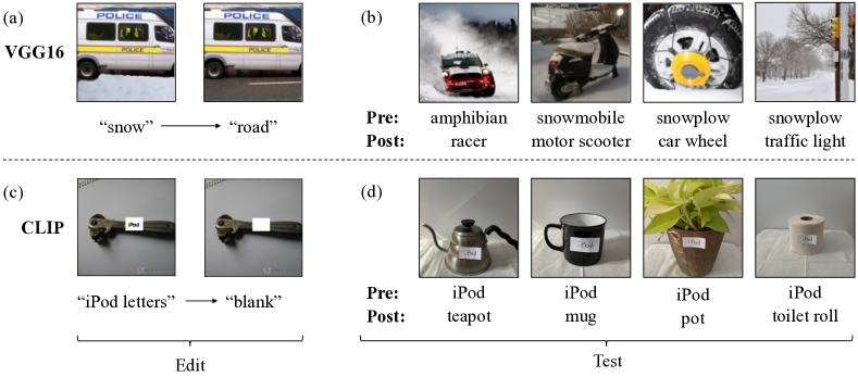
Figure 1: Editing prediction rules in pre-trained classifiers using a single exemplar. (a) We edit a VGG16 ImageNet classifier to map the representation of the concept “snow” to that of “asphalt road”. (b) This edit corrects classification errors on snowy scenes corresponding to various classes. (c) We edit a CLIP [RKH+21] model such that the text “iPod” maps to a blank area. (d) This change makes the model robust to the typographic attacks from [GCV+21].

Probing model behavior with counterfactuals.

Moving beyond model editing, we observe that the concept-transformation pipeline we developed can also be viewed as a scalable approach for generating image counterfactuals. In Section 5, we demonstrate how such counterfactuals can be useful to gain insights into how a given model makes its predictions and pinpoint certain spurious correlations that it has picked up.

2 A toolkit for editing prediction rules

It has been widely observed that models pick up various context-specific correlations in the data—e.g., using the presence of “road” or a “wheel” to predict “car” (cf. Section 5). Such unreliable prediction rules (dependencies of predictions on specific input concepts) could hinder models when they encounter novel environments (e.g., snow-covered roads), and confusing or adversarial test conditions (e.g., cars with wooden wheels). Thus, a model designer might want to modify these rules before deploying their model.

The canonical approach to modify a classifier post hoc is to collect additional data that captures the desired deployment scenario, and use it to retrain the model. However, even setting aside the challenges of data collection, it is not obvious a priori how much of an effect such retraining (e.g., via fine-tuning) will have. For instance, if we fine-tune our model on “cars” with wooden wheels, will it now recognize “scooters” or “trucks” with such wheels?

The goal of this work is to instead develop a more direct way to modify a model’s behavior: rewriting its prediction rules in a targeted manner. For instance, in our previous example, we would ideally be able to modify the classifier to correctly recognize all vehicles with wooden wheels by simply teaching it to treat any wooden wheel as it would a standard one. Our approach is able to do exactly this. However, before describing this approach (Section 2.2), we first provide a brief overview of recent work by [BLW+20] which forms its basis.

2.1 Background: Rewriting generative models

[BLW+20] developed an approach for rewriting a deep generative model: specifically, enabling a user to replace all occurrences of one selected object (say, “dome”) in the generated images with another (say, “tree”), without changing the model’s behavior in other contexts. Their approach is motivated by the observation that, using a handful of example images, we can identify a vector in the model’s representation space that encodes a specific high-level concept [KWG+18, BLW+20]. Building on this, [BLW+20] treat each layer of the model as an associative memory, which maps such a concept vector at each spatial location in its input (which we will refer to as the key) to another concept vector in its output (which we will call the value).

In the simplest case, one can think of a linear layer with weights $W\in\mathbb{R}^{mxn}$ transforming the key $k\in\mathbb{R}^{n}$ to the value $v\in\mathbb{R}^{m}$. In this setting, [BLW+20] formulate the rewrite operation as modifying the layer weights from $W$ to $W^{\prime}$ so that $v^{\ast}=W^{\prime}k^{\ast}$, where $k^{\ast}$ corresponds to the old concept that we want to replace, and $v^{\ast}$ to the new concept. For instance, to replace “domes” with “trees” in the generated images, we would modify the layer so that the key $k^{\ast}$ for “dome” maps to the value $v^{\ast}$ for “tree”. Consequently, when this value is fed into the downstream layers of the network it would result in a tree in the final image. Crucially, this update should change the model’s behavior for every instance of the concept encoded in $k^{\ast}$—i.e., all “domes” in the images should now be “trees”.

To extend this approach to typical deep generative models, two challenges remain: (1) handling non-linear layers, and (2) ensuring that the edit doesn’t significantly hurt model behavior on other concepts. With these considerations in mind, [BLW+20] propose making the following rank-one updates to the parameters $W$ of an arbitrary non-linear layer $f$:

$$\min_{\Lambda}\quad\sum_{(i,j)\in S}\left\|v^{\ast}_{ij}-f(k^{\ast}_{ij};W^{\prime})\right\|\qquad\text{s.t.}\quad W^{\prime}=W+\Lambda(C^{-1}d)^{\top}.$$ (1)

Here, $S$ denotes the set of spatial locations in representation space for a single image corresponding to the concept of interest, $d$ is the top eigenvector of the keys $k^{\ast}_{ij}$ at locations $(i,j)\in S$ and $C=\sum_{d}k_{d}{k_{d}}^{\top}$ captures the second-order statistics for other keys $k_{d}$. Intuitively, the goal of this update is to modify the layer parameters to rewrite the desired key-value mapping in the most minimal way. We refer the reader to [BLW+20] for further details.

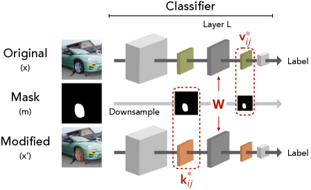
(a) Edit

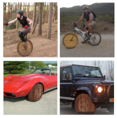
(b) Test

Figure 2: Overview of our pipeline for directly editing the prediction-rules of a classifier. The edit in (a) seeks to modify the network to perceive wooden wheels as standard ones, using a small set of exemplar images (say from class “car”). To achieve this, we first obtain the keys $k^{\ast}_{ij}$ corresponding to the new concept (here, “wooden wheel”), and the values $v^{\ast}_{ij}$ corresponding to the original concept (here, “standard wheel”) in the input and output representation space of a layer $L$ respectively. We then update the weights $W$ of the layer to enforce this new key-value association (1). (b) To test our method, we measure the improvement in model performance on test instances containing the new concept—here, images of other vehicles with “wooden wheels”.

2.2 Editing classifiers

We now shift our attention to the focus of this work: editing classifiers. To describe our approach, we use the task of enabling classifiers to detect vehicles with “wooden wheels” as a running example. At a high level, we would like to apply the approach described in Section 2.1 to modify a chosen (potentially non-linear) layer $L$ of the network to rewrite the relevant key-value association. But, we need to first determine what these relevant keys and values are.

Let us start with a single image $x$, say, from class “car”, that contains the concept “wheel”. Let the location of the “wheel” in the image be denoted by a binary mask $m$. Then, say we have access to a transformed version of $x$—namely, $x^{\prime}$—where the “car” has a “wooden wheel” (cf. Figure 2). This $x^{\prime}$ could be created by manually replacing the wheel, or by applying an automated procedure such as that in Section 4. In the rest of our study, we refer to a single ($x$, $x^{\prime}$) pair as an exemplar.

Intuitively, we want the classifier to perceive the “wooden wheel” in the transformed image $x^{\prime}$ as it does the standard wheel in the original image $x$. To achieve this, we must map the keys for wooden wheels to the value corresponding to their standard counterparts. In other words, the relevant keys ($k^{\ast}$) correspond to the network’s representation of the concept in the transformed image ($x^{\prime}$) directly before layer $L$. Similarly, the relevant values ($v^{\ast}$) that we want to map these keys to correspond to the network’s representation of the concept in the original images ($x$) directly after layer $L$. (The pertinent spatial regions in the representation space are simply determined by downsampling the mask to the appropriate dimensions.) Finally, the model edit is performed by feeding the resulting key-value pairs into the optimization problem (1) to determine the updated layer weights $W^{\prime}$—cf. Figure 2 for an illustration of the overall process. Note that this approach can be easily extended to use multiple exemplars $(x_{k},x^{\prime}_{k})$ by simply expanding $S$ to include the union of relevant spatial locations (corresponding the concept of interest) across these exemplars.

3 Does editing work in practice?

To test the effectiveness of our approach, we start by considering two scenarios motivated by real-world concerns: (i) adapting classifiers to handle novel weather conditions, and (ii) making models robust to typographic attacks [GCV+21]. In both cases, we edit the model using a single exemplar, i.e., a single image that we manually annotate and modify. For comparison, we also consider two variants of fine-tuning using the same exemplar: (i) local fine-tuning, where we only train the weights of a single layer $L$ (similar to our editing approach); and (ii) global fine-tuning, where we also train all other layers between layer $L$ and the output of the model. It is worth noting that unlike fine-tuning, our editing approach does not utilize class labels in any way. See Appendix A for experimental details.

3.1 Tackling new environments: Vehicles on snow

Our first use-case is adapting pre-trained classifiers to image subpopulations that are under-represented in the training data. Specifically, we focus on the task of recognizing vehicles under heavy snow conditions—a setting that could be pertinent to self-driving cars—using a VGG16 classifier trained on ImageNet-1k. To study this problem, we collect a set of real photographs from road-related ImageNet classes using Flickr (details in Appendix A.5). We then rewrite the model’s prediction rules to map “snowy roads” to “road”. To do so, we create an exemplar by manually annotating the concept “road” in an ImageNet image from a different class (here, “police van”), and the manually replace it with snow texture obtained from Flickr. We then apply our editing methodology (cf. Section 2), using this single synthetic snow-to-road exemplar—see Figure 1.

In Figure 3(a), we measure the error rate of the model on the new test set (vehicles in snow) before and after performing the rewrite. We find that our edits significantly improve the model’s error rate on these images, despite the fact that we only use a single synthetic exemplar (i.e., not a real “snowy road” photograph). Moreover, Figure 3(a) demonstrates that our method indeed changes the way that the model processes a concept (here “snow”) in a way that generalizes beyond the specific class used during editing (here, the exemplar was a “police van”) . In contrast, fine-tuning the model under the same setup does not improve its performance on these inputs.

One potential concern is the impact of this process on the model’s accuracy on other ImageNet classes that contain snow (e.g., “ski”). On the 246 (of 50k) ImageNet test images that contain snow (identified using an MS-COCO-trained instance segmentation model [CPK+17]), the model’s accuracy pre-edit is 92.27% and post-edit is 91.05%—i.e., only 3/246 images are rendered incorrect by the edit. This indicates that the classifier is not disproportionately affected by the edit.

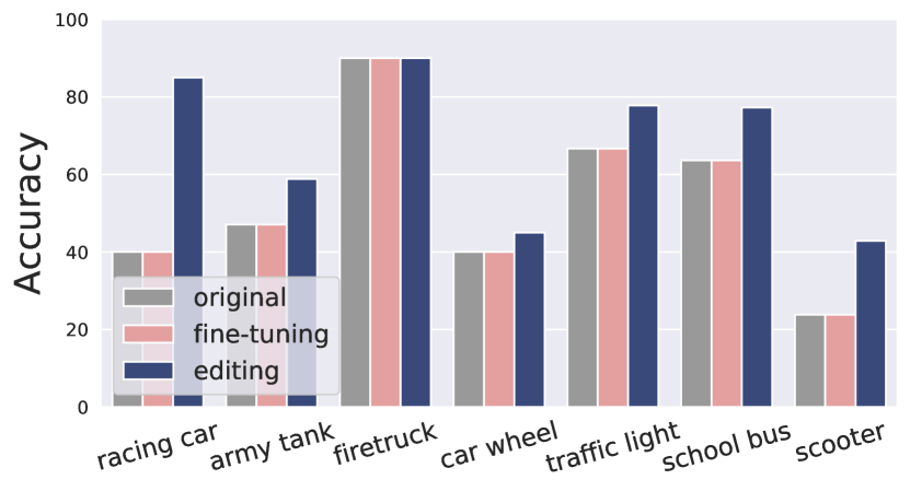
(a) Vehicles in snowy weather

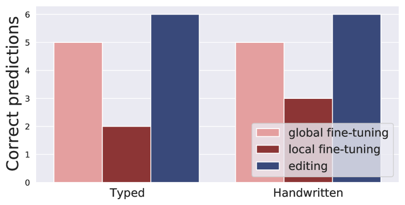
(b) Typographic attacks (6 images)

Figure 3: (a) Adapting a pre-trained ImageNet VGG16 classifier to images of vehicles on snowy roads with a single exemplar. Fine-tuning (both local and global) does not improve accuracy, while editing to map “snowy road”$\to$“road” leads to a consistent improvement across multiple classes. (b) Improving the robustness of CLIP-ResNet-50 [RKH+21] models to typographic attacks [GCV+21]. Editing the model to map the text “iPod”$\to$“blank” using a single exemplar—either based on hand-written text on a physical teapot or from pasting typed text on an image of a “can opener”—completely corrects this vulnerability. While global fine-tuning can also improve model performance in this setting, it requires more careful hyperparameter tuning and typically hurts model performance in other contexts (Appendix Figure 9). Here, hyperparameters (cf. Appendix Table 2) are chosen based on the large-scale synthetic study in Section 4.1.

3.2 Ignoring a spurious feature: Typographic attacks

Our second use-case is modifying a model to ignore a spurious feature. We focus on the recently-discovered typographic attacks from [GCV+21]: simply attaching a piece of paper with the text “iPod” on it is enough to make a zero-shot CLIP [RKH+21] classifier incorrectly classify an assortment of objects to be iPods. We reproduce these attacks on the ResNet-50 variant of the model—see Appendix Figure 7 for an illustration.

To correct this behavior, we rewrite the model’s prediction rules to map the text “iPod” to “blank”. For the choice of our transformed input $x^{\prime}$, we consider two variants: either a real photograph of a “teapot” with the typographic attack (Appendix Figure 7); or an ImageNet image of a “can opener” (randomly-chosen) with the typed text “iPod” pasted on it (Figure 1). The original image $x$ for our approach is obtained by replacing the handwritten/typed text with a white mask—cf. Figure 1. We then use this single training exemplar to perform the model edit.

In both cases, we find that editing is able to fix all the errors caused by the typographic attacks, see Figure 3(b). Interestingly, global fine-tuning also helps to correct many of these errors (potentially by adjusting class biases), albeit less reliably (for specific hyperparameters). However, unlike editing, fine-tuning also ends up damaging the model behavior in other scenarios—e.g., the model now spuriously associates the text “iPod” with the target class used for fine-tuning and/or has lower accuracy on normal “iPod” images from the test set (Appendix Figure 9).

4 Large-scale synthetic evaluation

The analysis of the previous section demonstrates that editing can improve model performance in realistic settings. However, due to the practical constraints of real-world data collection, this analysis was restricted to a relatively small test set. To corroborate the generality of our approach, we now develop a pipeline to automatically construct diverse rule-editing test cases. We then perform a large-scale evaluation and ablation of our editing method on this testbed.

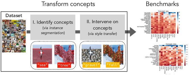
Figure 4: Creating large-scale test sets for model rewriting. Given a standard dataset, we first identify salient concepts within the corresponding images using instance segmentation, and then apply a realistic transformation to each of these concepts using style transfer [GEB16]. We can then evaluate the effectiveness of a model rewriting technique based on the extent to which it can alleviate the model’s sensitivity (i.e., drop in accuracy) to such concept-level transformations.

4.1 Synthesizing concept-level transformations

At a high level, our goal is to automatically create a test set(s) in which a specific concept—possibly relevant to the detection of multiple dataset classes—undergoes a realistic transformation. To achieve this without additional data collection, we transform all instances of the concept of interest within existing datasets. For example, the “vehicles-on-snow” scenario of Section 3.1 can be synthetically reproduced by identifying the images within a standard dataset (say ImageNet [DDS+09, RDS+15]) that contain segments of road and transforming these to make them resemble snow. Concretely, our pipeline (see Figure 4 for an illustration and Appendix A.6.1 for details), which takes as input an existing dataset, consists of the following two steps:

1. Concept identification: In order to identify concepts within the dataset images in a scalable manner, we leverage pre-trained instance segmentation models. In particular, using state-of-the-art segmentation models—trained on MS-COCO [LMB+14] and LVIS [GDG19]—we are able to automatically generate concept segmentations for a range of high-level concepts (e.g., “grass”, “sea”, “tree”).

2. Concept transformation: We then transform the detected concept (within dataset images) in a consistent manner using existing methods for style transfer [GEB16, GLK+17]. This allows us to preserve fine-grained image features and realism, while still exploring a range of potential transformations for a single concept. For our analysis, we manually curate a set of realistic transformations (e.g., “snow” and “graffiti”).

Note that this concept-transformation pipeline does not require any additional training or data annotation. Thus it can be directly applied to new datasets, as long as we have access to a pre-trained segmentation model for the concepts of interest.

4.2 Creating a suite of editing tasks

We now utilize the concept transformations described above to create a benchmark for evaluating model rewriting methods. Intuitively, these transformations can capture invariances that the model should ideally have—e.g., recognizing vehicles correctly even when they have wooden wheels. In practice however, model accuracy on one or more classes (e.g., “car”, “scooter”) may degrade under these transformations. The goal of rewriting the model would thus be to fix these failure modes in a data-efficient manner. In this section, we evaluate our editing methodology—as well as the fine-tuning approaches discussed in Section 3—along this axis.

Concretely, we focus on vision classifiers—specifically, VGG [SZ15] and ResNet [HZR+15] models trained on the ImageNet [DDS+09, RDS+15] and Places-365 [ZLK+17] datasets (cf. Appendix A.2). Each test set is constructed using the concept-transformation pipeline discussed above, based on a chosen concept-style pair (say “wheel”-“wooden”) . It consists of $N$ exemplars (pairs of original and transformed images, $(x,x^{\prime})$) that belong to a single (randomly-chosen) target class in the dataset. All other transformed images containing the concept, including those from classes other than the target one, are used for validation and testing (30-70 split). We create two variants of the test set: one using the same style image as the exemplars (i.e., same wooden texture) for the transformation; and another using held-out style images (i.e., other wooden textures).

To evaluate the impact of a method, we measure the change in model accuracy on the transformed examples (e.g., vehicles with “wooden wheel”s in Figure 2(b)). If the method is effective, then it should recover some of the incorrect predictions caused by the transformations. We only focus on the subset of examples $D$ that were correctly classified before the transformation, since we cannot expect to correct mistakes that do not stem from the transformation itself. Concretely, we measure the change in the number of mistakes made by the model on the transformed examples:

$$\text{\% errors corrected}:=\frac{N_{pre}(D)-N_{post}(D)}{N_{pre}(D)}$$ (2)

where $N_{pre/post}(D)$ denotes the number of transformed examples misclassified by the model before and after the rewrite, respectively. Note that this metric can range from 100% when rewriting leads to perfect classification on the transformed examples, to even a negative value when the rewriting process causes more mistakes that it fixes.

In each case, we select the best hyperparameters—including the choice of the layer to modify—based on the validation set performance (cf. Appendix A.6.3). To quantify the effect of the modification on overall model behavior, we also measure the change in its (standard) test set performance. Since we are interested in rewrites that do not significantly hurt the overall model performance, we only consider hyperparameters that do not cause a large accuracy drop ($\leq$0.25%). We found that the exact accuracy threshold did not have significant impact on the results—see Appendix Figures 15-18 for a demonstration of the full accuracy-effectiveness trade-off.

4.3 The effectiveness of editing

Recall that a key desideratum of our prediction-rule edits is that they should generalize. That is, if we modify the way that our model treats a specific concept, we want this modification to apply to every occurrence of that concept. For instance, if we edit a model to enforce that “wooden wheels” should be treated the same as regular “wheels” in the context of “car” images, we want the model to do the same when encountering other vehicles with “wooden wheels”. Thus, when analyzing performance in Figure 5, we consider inputs belonging to the class used to perform the edit separately.

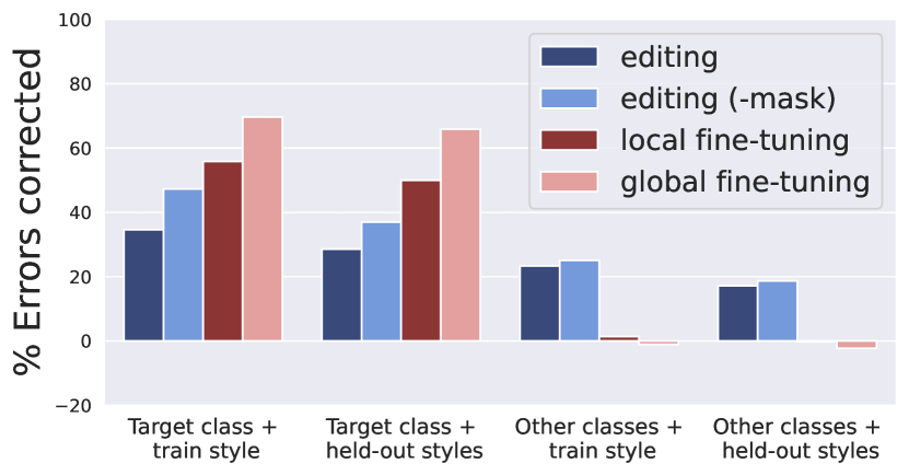
(a) ImageNet-trained VGG16 (concepts from COCO)

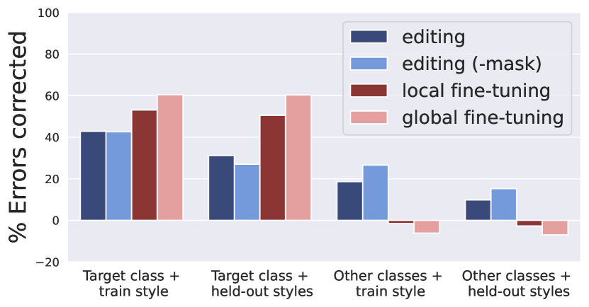
(b) Places-trained ResNet-18 (concepts from LVIS)

Figure 5: Editing vs. fine-tuning, averaged over concept-style pairs. We find that both methods (and their variants) are fairly successful at correcting misclassifications on the target class (examples of which are used to perform the rewrite). This holds even when the transformation applied during testing is different from the one present in the train exemplars (e.g., a different texture of “wood”). However, crucially, only the improvements induced by editing generalize to other classes where the transformed concept is present. Fine-tuning fails in this setting—typically, causing more errors than it fixes. See Appendix Figures 10-13 for other experimental settings.

Editing.

We find that editing is able to consistently correct mistakes in a manner that generalizes across classes. That is, editing is able to reduce errors in non-target classes, often by more than 20 percentage points, even when performed using only three exemplars from the target class. Moreover, this improvement extends to transformations using different variants of the style (e.g., textures of “wood”), other than those present in exemplars used to perform the modification.

In Appendix B.1.3, we conduct ablation studies to get a better sense of the key algorithmic factors driving performance. Notably, we find that imposing the editing constraints (1) on the entirety of the image—as opposed to only focusing on key-value pairs that correspond to the concept of interest as proposed in [BLW+20]—leads to even better performance (cf. ‘-mask’ in Figure 5). We hypothesize that this has a regularizing effect as it constrains the weights to preserve the original mapping between keys and values in regions that do not contain the concept.

Fine-tuning.

Our baseline is the canonical fine-tuning approach, i.e., directly minimizing the cross-entropy loss on the new data (in this case the transformed images) with respect to the target label. Similar to Section 3, we consider both the local and global variants of fine-tuning. We find that while these approaches are able to correct model errors on transformed inputs of the target class used to perform the modification, they typically decrease the model’s performance on other classes—i.e., they cause more errors than they fix. Moreover, even when we allow a larger drop in the model’s accuracy, or use more training exemplars, their performance often becomes worse on inputs from other classes (Appendix Figures 15-18).

We present examples of errors corrected (or not) by editing and fine-tuning in Appendix Figure 14, and provide a per-concept/style break down in Appendix Figures 19 and 20.

5 Beyond editing: Probing model behavior via counterfactuals

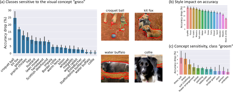
Figure 6: Model sensitivities diagnosed using our pipeline in a VGG16 classifier trained on ImageNet. (a) Classes for which the model relies on the concept “grass”: e.g., a “croquet ball” is not accurately recognized if “grass” is not present, while “collie”s are not affected. (We present the twenty classes for which the visual concept is most often.) (b) Applying different transformations (i.e., styles used for style transfer) to visual concepts reduces accuracy by varying amounts. (c) Visual concepts that cause accuracy losses for a given class can highlight prediction rules: e.g., the class “groom” is sensitive to the presence of “dress.”

In the previous section, we developed a scalable pipeline for creating concept-level transformations which we used to evaluate model rewriting methods. Here, we put forth another related use-case of that pipeline: debugging models to identify their (learned) prediction rules.

In particular, observe that the resulting transformed inputs (cf. Figure 4) can be viewed as counterfactuals—a primitive commonly used in causal inference [Pea10] and interpretability [GFS+19, GWE+19, BZS+20]. Counterfactuals can be used to identify the features that a model uses to make its prediction on a given input. For example, to understand whether the model relies on the presence of a “wheel” to recognize a “car” image, we can evaluate how the its prediction changes when just the wheel in the image is transformed. Based on this view, we now repurpose our concept transformations from Section 4 to discover a given classifier’s prediction rules.

The effect of specific concepts.

As a point of start, we study how sensitive the model’s prediction is to a given high-level concept—in terms of the accuracy drop caused by transformation of said concept. For instance, in Figure 6a, we find that the accuracy of a VGG16 ImageNet classifier drops by 25% on images of “croquet ball” when “grass” is transformed, whereas its accuracy on “collie” does not change. In line with previous studies [ZML+07, RSG16, RZT18, BMA+19, XEI+20], we also find that background concepts, such as “grass”, “sea” and “sand”, have a large effect on model performance. We can contrast this measure of influence across concepts for a single model (Appendix Figure 27), and across architectures for a single concept (Appendix B.2). Finally, we can also examine the effect of specific transformations to a single concept—cf. Figure 6b.

Per-class prediction rules.

If instead we restrict our attention to a single class, we can pinpoint the set of concepts that the model relies on to detect this class. It turns out that aside from the main image object, ImageNet classifiers also heavily depend on commonly co-occurring objects [SC18, TSE+20, BHK+20] in the image—e.g., “dress” for the class “groom”, “person” for the class “tench” (sic), and “road” for the class “race car” (cf. Figure 6c and Appendix Figure 29). We can also examine which transformations hurt model performance on the given class most substantially—e.g., we find that making “plants” “floral” hurts accuracy on the class “damselfly” 15% more than making them “snowy”.

Overall, this pipeline provides a scalable path for model designers to analyze the invariances (and sensitivities) of their models with respect to various natural transformations of interest. We thus believe that this primitive holds promise for future interpretability and robustness studies.

6 Related work

High-level concepts in latent representations. There has been increasing interest in explaining the inner workings of deep classifiers through high-level concepts: e.g., by identifying individual neurons [EBC+09, ZF14, OMS17, BZK+17, EIS+19] or activation vectors [KWG+18, ZSB+18, CBR20] that correspond to human-understandable features. The effect of these features on model predictions can be analyzed by either inspecting the downstream weights of the model [OSJ+18, WSM21] or through counterfactual tests: e.g., via synthetic data [GFS+19]; by swapping features between individual images [GWE+19]; or by silencing sets of neurons [BZS+20]. A parallel line of work aims to learn models that operate on data representations that explicitly encode high-level concepts: either by learning to predict a set of attributes [LNH09, KNT+20] or by learning to segment inputs [LFS19]. In our work, we identify concepts by manually selecting the relevant pixels in a handful of images and measure the impact of manipulating these features on model performance on a new test set.

Model interventions.

Direct manipulations of latent representations inside generative models have been used to create human-understandable changes in synthesized images [BZS+19, JCI19, GAO+19, SGT+20, HHL+20, WLS20]. Our work is inspired by that line of work as well as a recent finding that parameters of a generative model can be directly changed to alter generalized behavior [BLW+20]. Unlike previous work, we edit classification models, changing rules that govern predictions rather than image synthesis. Concurrently with our work, there has been a series of methods proposed for editing factual knowledge in language models [MLB+21, DAT21, DDH+21].

Ignoring spurious features.

Prior work on preventing models from relying on spurious correlations is based on constraining model predictions to satisfy certain invariances. Examples include: training on counterfactuals (either by adding or removing objects from scenes [SFS18, SSF19, ASF20] or having human annotators edit text input [KHL19]), learning representations that are simultaneously optimal across domains [ABG+19], ensuring comparable performance across subpopulations [SKH+20], or enforcing consistency across inputs that depict the same entity [HM17]. In this work, we focus on a setting where the model designer is aware of undesirable correlations learned by the model and we provide the tools to rewrite them directly.

Model robustness.

A long line of work has been devoted to discovering and correcting failure modes of models. These studies focus on simulating variations in testing conditions that can arise during deployment, including: adversarial or natural input corruptions [SZS+14, FF15, FMF16, ETT+19, FGC+19, HD19, KSH+19], changes in the data collection process [SKF+10, TE11, KZM+12, TT14, RRS+19], or variations in the data subpopulations present [BVP18, OSH+19, SKH+20, STM21, KSM+20]. Typical approaches for improving robustness in these contexts include robust optimization [MMS+18, YLS+19, SKH+20] and data augmentation schemes [LYP+19, HMC+19, ZDK+21]. Our rule-discovery and editing pipelines can be viewed as complementary to this work as they allows us to preemptively adjust the model’s prediction rules in anticipation of deployment conditions.

Domain adaptation.

The goal of domain adaptation is to adapt a model to a specific deployment environment using (potentially unlabeled) samples from it. This is typically achieved by either fine-tuning the model on the new domain [DJV+14, SAS+14, KML20], learning the correspondence between the source and target domain, often in a latent representation space [BBC+07, SKF+10, GL15, CFT+16, GZL+16], or updating the model’s batch normalization statistics [LWS+16, BS21]. These approaches all require a non-trivial amount of data from the target domain. The question of adaptation from a handful of samples has been explored [MJI+17], but in a setting that requires samples across all target classes. In contrast, our method allows for generalization to new (potentially unknown) classes with even a single example.

7 Conclusion

We developed a general toolkit for performing targeted post hoc modifications to vision classifiers. Crucially, instead of specifying the desired behavior implicitly via the training data, our method allows users to directly edit the model’s prediction rules. By doing so, our approach makes it easier for users to encode their prior knowledge and preferences during the model debugging process. Additionally, a key benefit of this technique is that it fundamentally changes how the model processes a given concept—thus making it possible to edit its behavior beyond the specific class(es) used for editing. Finally, our edits do not require any additional data collection: they can be guided by as few as a single (synthetically-created) exemplar. We believe that this primitive opens up new avenues to interact with and correct our models before or during deployment.

Limitations and broader impact.

Even though our methodology provides a general tool for model editing, performing such edits does require manual intervention and domain expertise. After all, the choice of what concept to edit—and its implications on the robustness of the model—lies with the model designer. For instance, in the vehicles-on-snow example, our objective was to have the model recognize any vehicle on snow the same way it would on a regular road—e.g., to adapt a system to different weather conditions. However, if our dataset contains classes for which the presence snow is absolutely essential for recognition, this might not be an appropriate edit to perform.

Moreover, direct model editing is a departure from the standard way in which models are trained, and may have broader implications. While we have shown how it can be used to cause beneficial changes in pre-trained models, direct control of prediction rules could also make it easier for adversaries to introduce vulnerabilities into the model (e.g., by manipulating model behavior on a specific population demographic). Overall, direct model editing makes it clearer than ever that our models are a reflection of the goals and biases of we who create them—not only through the training tasks we choose, but now also through the rules that we rewrite.

8 Acknowledgements

We thank the anonymous reviewers for their helpful comments and feedback.

Work supported in part by the NSF grants CCF-1553428 and CNS-1815221, the DARPA SAIL-ON HR0011-20-C-0022 grant, Open Philanthropy, a Google PhD fellowship, and a Facebook PhD fellowship. This material is based upon work supported by the Defense Advanced Research Projects Agency (DARPA) under Contract No. HR001120C0015.

Research was sponsored by the United States Air Force Research Laboratory and the United States Air Force Artificial Intelligence Accelerator and was accomplished under Cooperative Agreement Number FA8750-19-2-1000. The views and conclusions contained in this document are those of the authors and should not be interpreted as representing the official policies, either expressed or implied, of the United States Air Force or the U.S. Government. The U.S. Government is authorized to reproduce and distribute reprints for Government purposes notwithstanding any copyright notation herein.

Appendix A Experimental Setup

A.1 Datasets

For the bulk of our experimental analysis (Sections 4 and 5) we use the ImageNet-1k [DDS+09, RDS+15] and Places-365 [ZLK+17] datasets which contain images from 1,000 and 365 categories respectively. In particular, both prediction-rule discovery and editing are performed on samples from the standard test sets to avoid overlap with the training data used to develop the models.

Licenses.

Both datasets were collected by scraping online image hosting engines and, thus, the images themselves belong to their individuals who uploaded them. Nevertheless, as per the terms of agreement for each dataset , these images can be used for non-commercial research purposes.

A.2 Models

Here, we describe the exact architecture and training process for each model we use. For most of our analysis, we utilize two canonical, yet relatively diverse model architectures for our study: namely, VGG [SZ15] and ResNet [HZR+16]. We use the standard PyTorch implementation  and train the models from scratch on the ImageNet and Places365 datasets. The accuracy of each model on the corresponding test set is provided in Table 1.

ImageNet classifiers.

We study: (i) a VGG16 variant with batch normalization and (ii) a ResNet-50. Both models are trained using standard hyperparameters: SGD for 90 epochs with an initial learning rate of 0.1 that drops by a factor of 10 every 30 epochs. We use a momentum of 0.9, a weight decay of $10^{-4}$ and a batch size of 256 for the VGG16 and 512 for the ResNet-50.

Places365 classifiers.

We study: (i) a VGG16 and (ii) a ResNet-18. Both models are trained for 131072 iterations using SGD with a single-cycle learning rate schedule peaking at 2e-2 and descending to 0 at the end of training. We use a momentum 0.9, a weight decay 5e-4 and a batch size of 256 for both models.

CLIP.

For the typographic attacks of Section 3, we use the ResNet-50 models trained via CLIP [RKH+21], as provided in the original model repository.

	Test Accuracy (%)
Architecture $\backslash$ Dataset	ImageNet	Places
VGG	73.70	54.02
ResNet	75.77	54.24
CLIP-ResNet	59.84	-

Table 1: Accuracy of each model architecture on the datasets used in our analysis.

A.3 Compute

Our experiments were performed on our internal cluster, comprised mainly of NVIDIA 1080Ti GTX GPUs. For the rule-discovery pipeline, we only need to evaluate models on images where the corresponding object is present, which allows us to perform the evaluation on a single style in less than 8 hours on a single GPU (amortized over concepts and classes). For the model rewriting process, each instance of editing or fine-tuning takes a little more than a minute, since it only operates on a section of the model and using a handful of training examples.

A.4 Model rewriting

Here, we describe the training setup of our model editing process, as well as the fine-tuning baseline. Recall that these rewrites are performed with respect to a single concept-style pair.

Layers.

We consider a layer to be a block of convolution-BatchNorm-ReLU, similar to [BLW+20] and rewrite the weights of the convolution. For ResNets (which were not previously studied), we must also account for skip connections. In particular, note that the effect of a rewrite to a layer inside any residual block will be attenuated (or canceled) by the skip connection. To avoid this, we only rewrite the final layer within each residual block—i.e., focus on the convolution-BatchNorm-ReLU right before a skip connection, and include the skip connection in the output of the layer. Unless otherwise specified, we perform rewrites to layers $[8,10,11,12]$ for VGG models, $[4,6,7]$ for ResNet-18, and $[8,10,14]$ for ResNet-50 models. We tried earlier layers in our initial experiments, but found that both methods perform worse.

A.4.1 Editing

We use the ADAM optimizer with a fixed learning rate to perform the optimization in (1). We grid over different learning rate-number of step pairs: $[(10^{-3},10k)$, $(10^{-4},20k)$, $(10^{-5},40k)$, $(10^{-6},80k)$, $(10^{-7},80k)]$. The second order statistics (cf. Section 2) are computed based on the keys for the entire test set.

A.4.2 Fine-tuning

When fine-tuning a single layer (local fine-tuning), we optimize the weights of the convolution of that particular layer. Instead, when we fine-tune a suffix of the model (global fine-tuning), we optimize all the trainable parameters including and after the chosen layer. In both cases, we use SGD, griding over different learning rate-number of step pairs: $[(10^{-2},500)$, $(10^{-3},500)$, $(10^{-4},500)$, $(10^{-5},800)$, $(10^{-6},800)]$. We verified that in all cases the optimal performance of the method was achieved for hyperparameters strictly within that range and thus performing more steps would not provide any benefits.

A.5 Real-world test cases

In Section 3 we study two real-world applications of our model rewriting methodology. Below, we outline the data-collection process for each case as well as the hyperparameters used.

Vehicles on snow.

We manually chose a subset of Imagenet classes that frequently contain “roads”, identified using our prediction-rule discovery pipeline in Section 4. In particular, we focus on the classes: “racing car”, “army tank”, “fire truck”, “car wheel”, “traffic light”, “school bus”, and “motor scooter”. For each of these classes, we searched Flickr using the query “$<$class name$>$ on snow” and manually selected the images that clearly depicted the class and actually contained snowy roads. We were able to collect around 20 pictures for each class with the exception of “traffic light” where we only found 9.

Typographic attacks.

We picked six household objects corresponding to ImageNet classes, namely: “teapot”, “mug”, “flower pot”, “toilet tissue”, “vase”, and “wine bottle”. We used a smartphone camera to photograph each of these objects against a plain background. Then, we repeated this process but after affixing a piece of paper with the text “iPod” handwritten on it, as well as when affixing a blank piece of paper—see Figure 7.

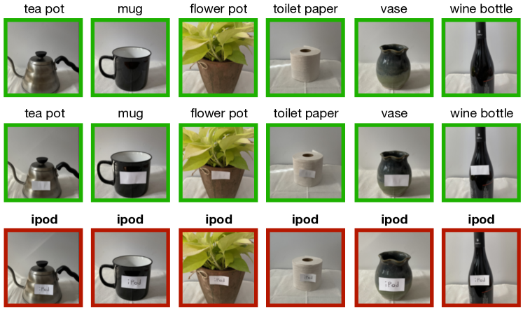
Figure 7: Typographic attacks on CLIP: We reproduce the results of [GCV+21] by taking photographs of household objects with a paper containing handwritten text “iPod” attached to them (third row). We see that these attacks consistently fool the zero-shot CLIP classifier (ResNet-50)—compare the predictions (shown in the title) for the first and third row. In contrast, if we instead use a blank piece of paper (second row), the model predicts correctly.

Hyperparameters.

Since our manually collected test sets are rather small, we decided to avoid tuning hyperparameters on them as this would require holding out a non-trivial number of data points. Instead, we inspected the results of the large-scale synthetic evaluation and manually picked values that performed consistently well which we list in Table 2. Nevertheless, we found that the results would be quite similar if we tuned hyperparameters directly on these test sets.

Model	Method	# steps	Step size	Layer	Mask
VGG16	Editing	20,000	1e-4	12 (last)	No
	Fine-tuning	400	1e-4	12 (last)	N/A
CLIP-ResNet-50	Editing	20,000	1e-4	14 (last)	No
	Fine-tuning	800	1e-5	14 (last)	N/A

Table 2: Hyperparameters chosen for evaluating on the real-world test cases.

A.6 Synthetic evaluation

We now describe the details of our evaluation methodology, namely, how we transform inputs, how we chose which concept-style pairs to use for testing and how we chose the hyperparameters for each method.

A.6.1 Creating concept-level transformations

Recall that our pipeline for transforming concepts consists of two steps: concept detection and concept transformation (Section 4). We describe each step below and provide examples in Figure 8.

We detect concepts using pre-trained object detectors trained on MS-COCO [LMB+14] and LVIS [GDG19]. For MS-COCO, we use a model with a ResNet-101 backbone which is trained on COCO-Stuff annotations and can detect 182 concepts [CPK+17]. For LVIS, we use a pre-trained model from the Detectron [GRG+18] model zoo, which can detect 1230 classes. We only consider a prediction as valid for a specific pixel if the model’s predicted probability is at least 0.80 for the COCO-based model and 0.15 for the LVIS-based model (chosen based on manual inspection). Moreover, we treat a concept as present in a specific image if it present in at least 100 pixels (image size is 224$\times$224 for ImageNet and 256$\times$256 for Places).

In order to transform concepts, we utilize the fast style transfer methodology of [GLK+17] using their pre-trained model. This allows us to quickly apply the same style to a large number of images which is ideal for our use-case. Specifically, we manually choose 14 styles (illustrated in Figure 8) and choose 3 images for each. This allows us to perform the concept-level transformation in several ways and evaluate how sensitive our model is to the exact style used.

All the pre-trained models used are open-sourced and available for non-commercial research.

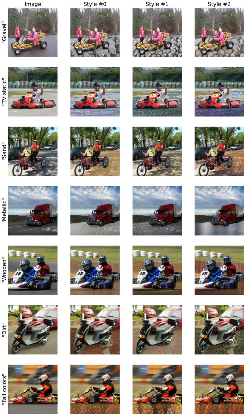
(a)

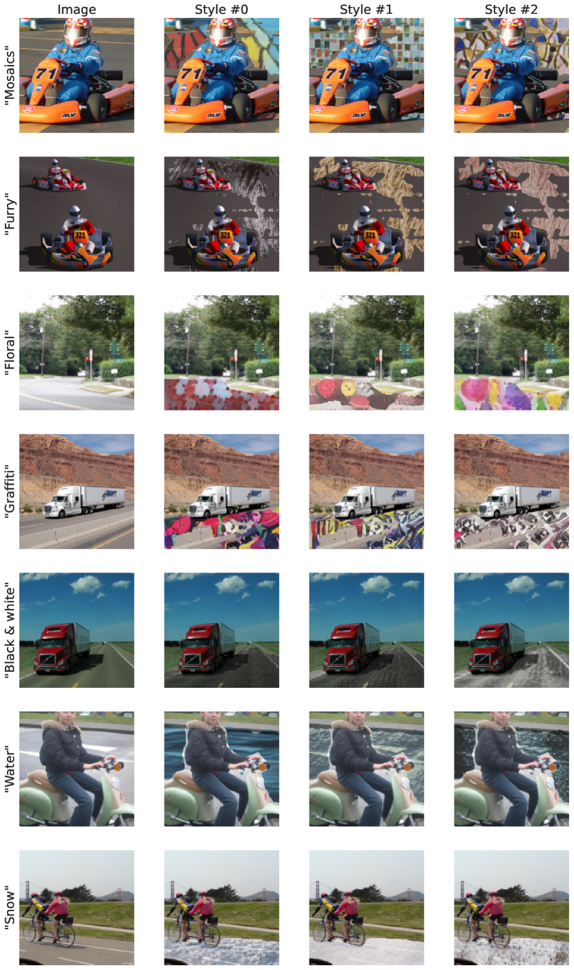
(b)

Figure 8: Illustration of concept-level transformations in ImageNet: We transform the concept “road” in images belonging to various classes via style transfer. Each row (within (a) and (b)) depicts the stylization of a single image with respect to the style described in the label (e.g., “gravel”). We collect three examples per style, which are then split across training and testing.

A.6.2 Selecting concept-style pairs

Concept selection.

Recall that our transformation pipeline from Section 4 identifies concepts which, when transformed in a certain manner hurts model accuracy on one or more classes. We first filter these concepts (automatically) to identify ones that are particularly salient in the model’s prediction-making process. In particular, we focus on concepts which simultaneously: (a) affect at least 3 classes; (b) are present in at least 20% percent of the test images of each class; and (c) cause a drop of at least 15% among these images. This selection results in a test bed where we can meaningfully observe differences in performance between approaches.

At the same time, we need to also ensure that the rewriting task we are solving is meaningful. For instance, if we replace all instances of “dog” with a stylized version, then distinguishing between a “terrier” and a “poodle” can become challenging (or even impossible). Moreover, we cannot expect the performance of the model to improve on other dog breeds if we modify it to treat a stylized dog as a “terrier”. To eliminate such test cases, we manually filter the concept-class pairs flagged by our prediction-rule discovery pipeline. In particular, we removed those where the detected concept overlapped significantly with the class object itself. In other words, if the concept detected is essential for correctly recognizing the class of the image, we exclude it from our analysis. Typical examples of excluded concept-class pairs on ImageNet include broad animal categories (e.g., “bird” or “dog”) for classes corresponding to specific breeds (e.g., “parrot”) or the concept “person” which overlaps with classes corresponding to articles of clothing (e.g., “suit”).

Style selection.

We consider a subset of 8 styles for our analysis: “black and white”, “floral”, “fall colors”, “furry”, “graffiti”, “gravel”, “snow” and “wooden”. While performing editing with respect to a single concept-style pair—say “wheel”-“wooden”—we randomly select one wooden texture to create train exemplars and hold out the other two for testing (described as held-out styles in the figures).

A.6.3 Hyperparameter selection

As discussed in Appendix A.4, for a particular concept-style pair, we grid over different hyperparameters pertaining to the rewrite (via editing or fine-tuning)—in particular the layer that is modified, as well as training parameters such as the learning rate. For our evaluation, we then choose a single set of hyperparameters (per concept-style pair). At a high level, our objective is to find hyperparameters that improve model performance on transformed examples, while also ensuring that the test accuracy of the model does not drop below a certain threshold. To this end, we create a validation set per concept-style pair with 30% of the examples containing this concept (and transformed using the same style as the train exemplars). We then use the performance on that subset (2) to choose the best set of hyperparameters. If all of the hyperparameters considered cause accuracy to drop below the specified threshold, we choose to not perform the edit at all. We then report the performance of the method on the test set (the other 70% of samples containing this concept).

A.7 Data ethics

Since we manually collected all the data necessary for our analysis in Section 3, we were able to filter them for offensive content. Moreover, we made sure to only collect images that are available under a Creative Commons license (hence allowing non-commercial use with proper attribution).

For the rest of our analysis, we relied on publicly available datasets that are commonly used for image classification. Unfortunately, due to their scale, these datasets have not been thoroughly filtered for offensive content or identifiable information. In fact, improving these datasets along this axis is an active area of work. Nevertheless, since our research did not involve redistributing these datasets or presenting them to human annotators, we did not perceive any additional risks that would result from our work.

Appendix B Additional Experiments

B.1 Fine-grained model behavior on typographic attacks

In Figure 9, we take a closer look at how effective different rewriting methods (with one train exemplar) are in mitigating typographic attacks. We find that:

• Local-finetuning: Corrects only a subset of the errors.

• Global-finetuning: Corrects most errors on the attacked images. However, on the flip side it: (i) causes the model to spuriously associate other images with the target class (“teapot”) used to perform fine-tuning and (ii) significantly reduces model accuracy on clean images of the class “iPod”.

• Editing: Corrects all errors without substantially hurting model accuracy on clean images.

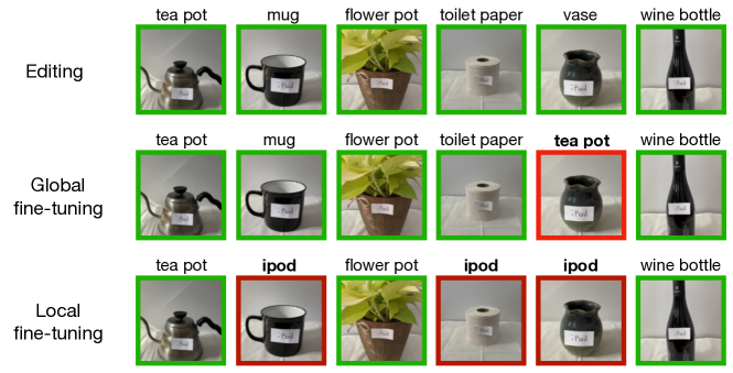
(a)

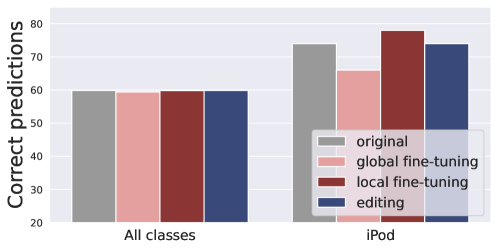
(b)

Figure 9: Effectiveness of different modification procedures in preventing typographic attacks. (a) Model predictions after the rewrite—local fine-tuning often fails to prevent such attacks, while global fine-tuning results in the model associating “iPod” with the target class used for fine-tuning (“teapot”). (b) Accuracy on the original test set and specifically on clean samples from class “ipod” before and after the rewrite. While global fine-tuning is fairly effective at mitigating typographic attacks, it disproportionately reduces model accuracy on clean images from the “iPod” class.

B.1.1 The effectiveness of editing

In Figures 10- 13, we compare the generalization performance of editing and fine-tuning (and their variants)—for different datasets (ImageNet and Places), architectures (VGG16 and ResNets) and number of exemplars (3 and 10). In performing these evaluations, we only consider hyperparameters (for each concept-style pair) that do not drop the overall (test set) accuracy of the model by over 0.25%. The complete accuracy-performance trade-offs of editing and fine-tuning (and their variants) are illustrated in Appendix Figures 15-18.

We observe that both methods successfully generalize to held-out samples from the target class (used to perform the modification)—even when the transformation is performed using held-out styles. However, while the performance improvements of editing also extend to other classes containing the same concept, this does not seem to be the case for fine-tuning. These trends hold even when we use more exemplars to perform the modification. In Appendix Figure 14, we illustrate sample error corrections (and failures to do so) due to editing and fine-tuning.

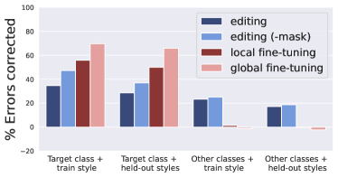
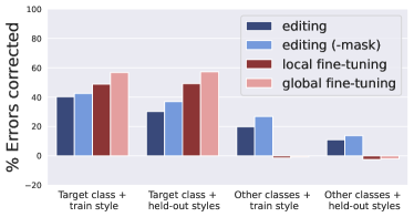
(a) $3$ training exemplars

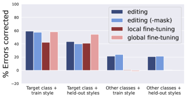
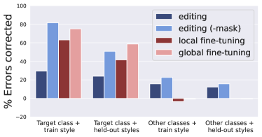
(b) $10$ training exemplars

Figure 10: Editing vs. fine-tuning: average number of misclassifications corrected by the method when applied to an ImageNet-trained VGG16 classifier. Here, the average is computed over different concept-transformation pairs—with concepts derived from instance segmentation modules trained on MS-COCO (left) and LVIS (right); and transformations described in Appendix A.4.1. For both editing and fine-tuning, the overall drop in model accuracy is less than $0.25\%$.

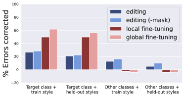
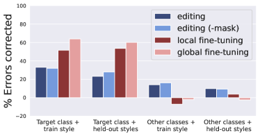
(a) $3$ training exemplars

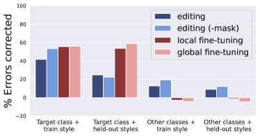
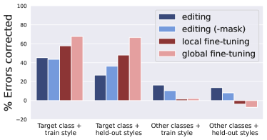
(b) $10$ training exemplars

Figure 11: Repeating the analysis in Appendix Fig. 10 on an ImageNet-trained ResNet-50 classifier.

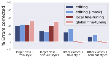
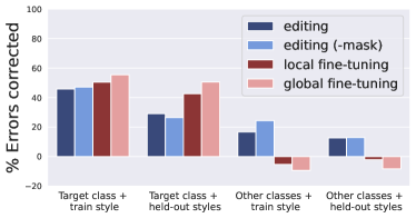
(a) $3$ training exemplars

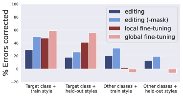
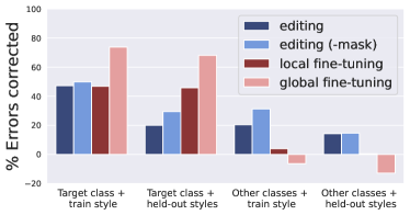
(b) $10$ training exemplars

Figure 12: Repeating the analysis in Appendix Fig. 10 on an Places365-trained VGG16 classifier.

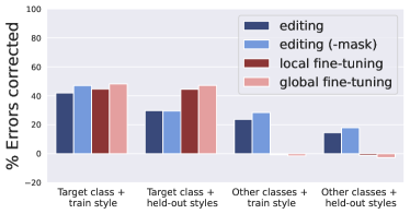
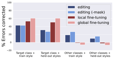
(a) $3$ training exemplars

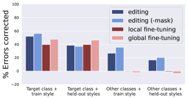
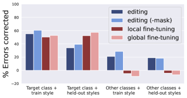
(b) $10$ training exemplars

Figure 13: Repeating the analysis in Appendix Fig. 10 on an Places365-trained ResNet-18 classifier.

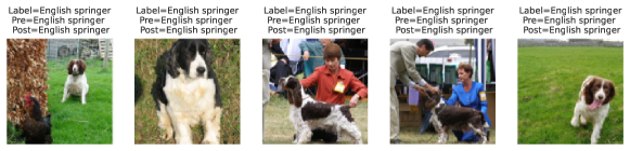
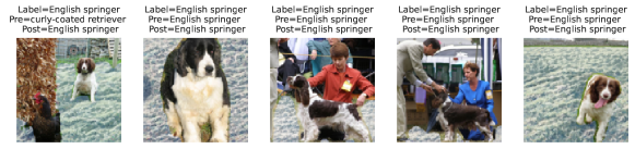
(a) Train exemplars: (top) Original and (bottom) transformed images.

Method: Fine-tuning

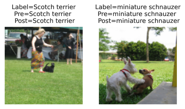
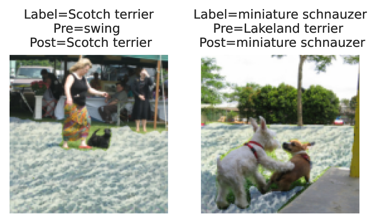
(b) Corrections (3.12%)

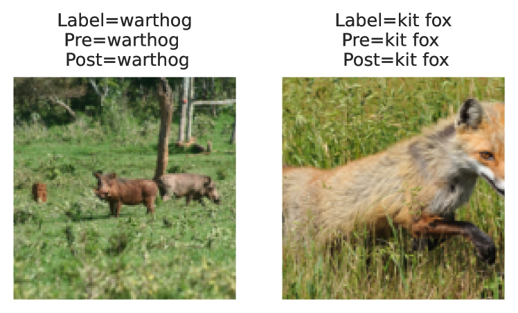
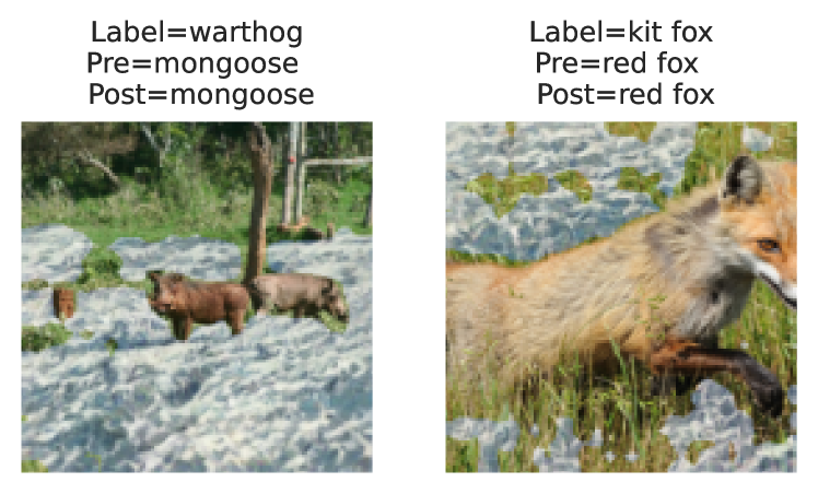
(c) No change (85.63%)

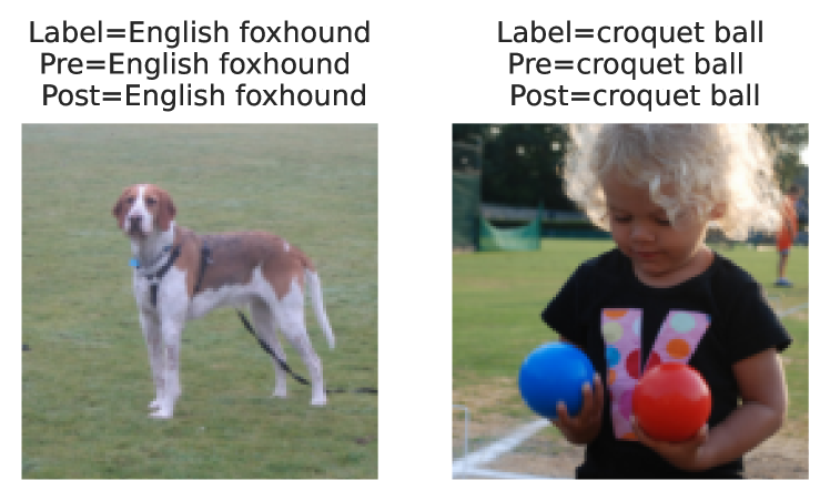
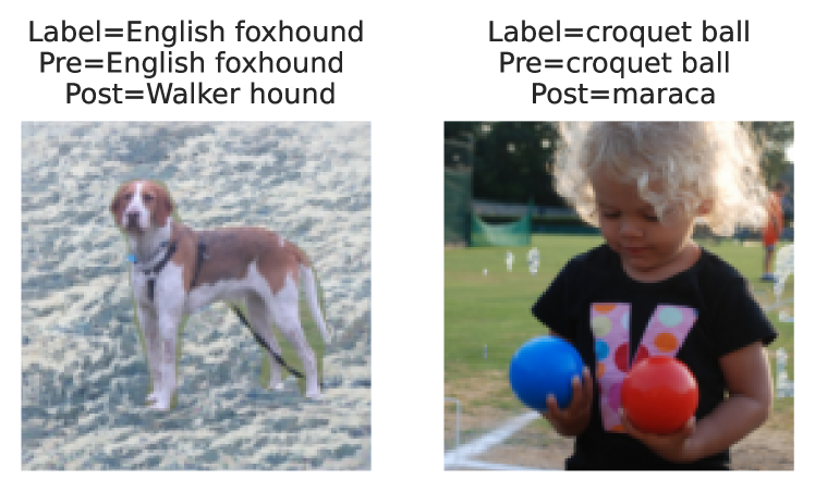
(d) New errors (11.25%)

Method: Editing

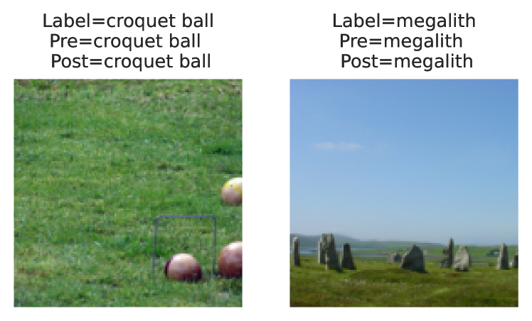
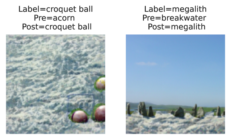
(e) Corrections (32.89%)

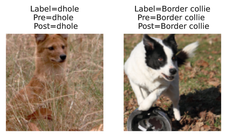
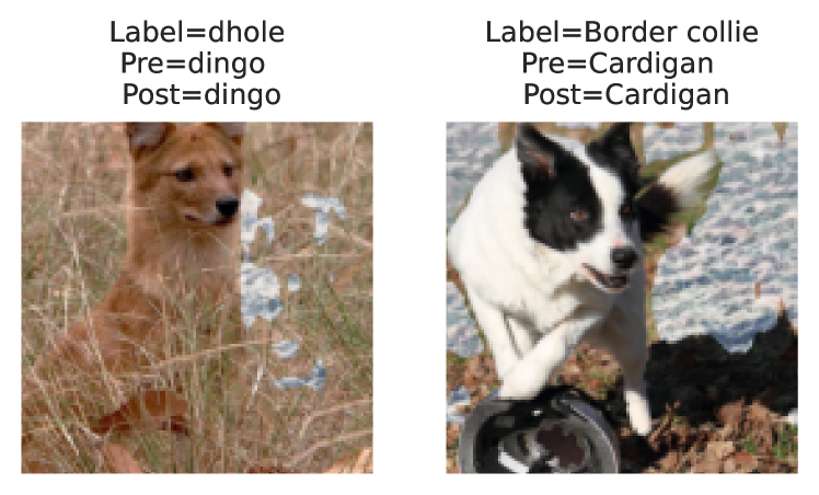
(f) No change (59.87%)

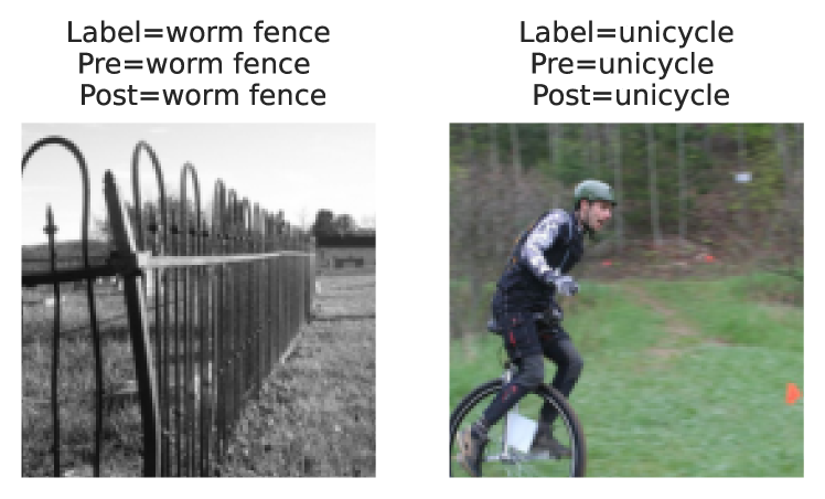
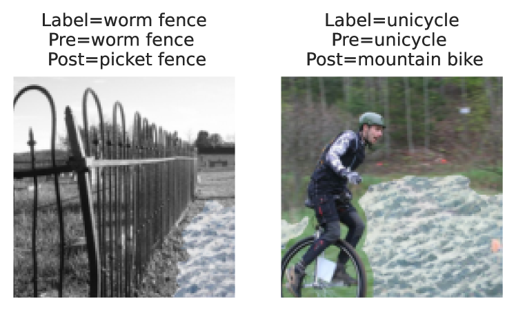
(g) New errors (7.24%)

Figure 14: Examples of errors (not) corrected by the rewrite: Here, the goal is to improve the accuracy of a VGG16 model when “grass” in ImageNet images is replaced with “snow”. The true label and the pre/post-edit predictions for each image are in the title. (a) Train exemplars for editing and fine-tuning. Test set examples where fine-tuning and editing correct the model error on the transformed example (b/e), do not cause any change (c/f) and induce an new error (d/g). The number in parenthesis indicates the fraction of the test set that falls into each of these subsets.

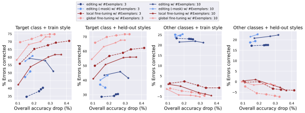
(a) Concepts derived from an instance segmentation model trained on MS-COCO.

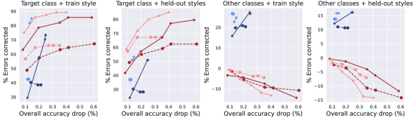
(b) Concepts derived from an instance segmentation model trained on LVIS.

Figure 15: Performance vs. drop in overall test set accuracy: Here, we visualize average number of misclassifications corrected by editing and fine-tuning when applied to an ImageNet-trained VGG16 classifier—where the average is computed over different concept-transformation pairs.

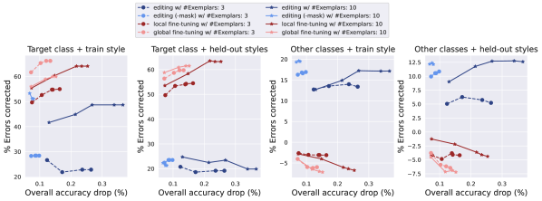
(a) Concepts derived from an instance segmentation model trained on MS-COCO.

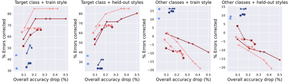
(b) Concepts derived from an instance segmentation model trained on LVIS.

Figure 16: Repeating the analysis in Appendix Fig. 15 on an ImageNet-trained ResNet-50 classifier.

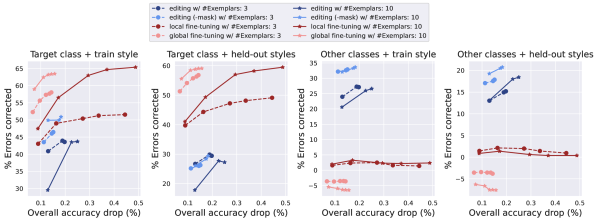
(a) Concepts derived from an instance segmentation model trained on MS-COCO.

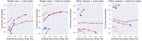
(b) Concepts derived from an instance segmentation model trained on LVIS.

Figure 17: Repeating the analysis in Appendix Fig. 15 on an Places365-trained VGG16 classifier.

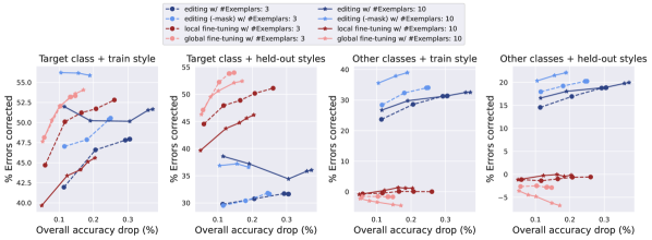
(a) Concepts derived from an instance segmentation model trained on MS-COCO.

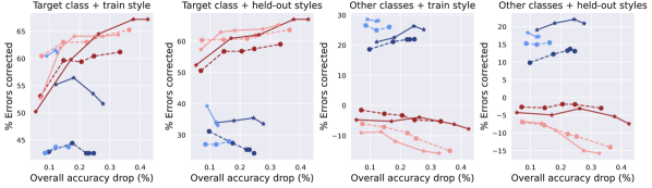
(b) Concepts derived from an instance segmentation model trained on LVIS.

Figure 18: Repeating the analysis in Appendix Fig. 15 on an Places365-trained ResNet-18 classifier.

B.1.2 A fine-grained look at performance improvements

In Appendix Figures 19 and 20 we take a closer look at the performance improvements caused by editing (-mask) and (local) fine-tuning (with 10 exemplars) on an ImageNet-trained VGG16 classifier. In particular, we break down the improvements on test examples from non-target classes with the same transformation as training, per-concept and per-style respectively. As before, we only consider hyperparameters that lead to an overall accuracy drop of less than $0.25\%$.

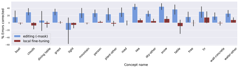
(a) Concepts derived from an instance segmentation model trained on MS-COCO.

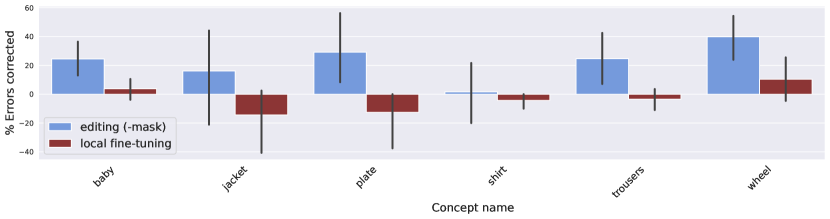
(b) Concepts derived from an instance segmentation model trained on LVIS.

Figure 19: Performance of editing and fine-tuning on test examples from non-target classes containing a given concept, averaged across transformations (cf. Appendix A.4.1).

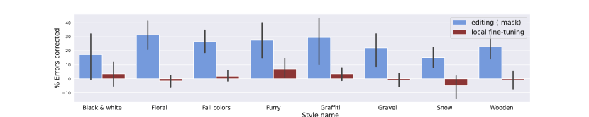
(a) Concepts derived from an instance segmentation model trained on MS-COCO.

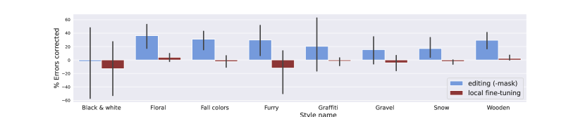
(b) Concepts derived from an instance segmentation model trained on LVIS.

Figure 20: Performance of editing and fine-tuning on test examples from non-target classes transformed using a given style, averaged across concepts.

B.1.3 Ablations

In order to get a better understanding of the core factors that affect performance in this setting, we conduct a set of ablation studies. Note that we can readily perform these ablations as, in contrast to the setting of [BLW+20] we have access to a quantitative performance metric that does not rely on human evaluation.

Layer. We compare both editing and local fine-tuning when they are applied to different layers of the model in Appendix Figure 21. For editing, we find a consistent increase in performance—on examples from both the target and other classes—as we edit deeper into the model. For (local) fine-tuning, a similar trend is observed with regards to performance on the target class, with the second last layer being optimal overall. However, at the same time, the fine-tuned model’s performance on examples from other classes containing the concept seems to get worse.

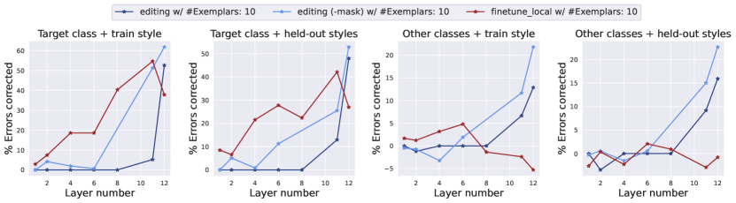
Figure 21: Editing vs. fine-tuning performance (with 10 exemplars) on an ImageNet-trained VGG16 classifier, as a function of the layer that is modified. Here, we visualize the average number of misclassifications corrected over different concept-transformation pairs, with concepts derived from instance segmentation modules trained on MS-COCO; and transformations “snow” and “graffiti”. For both editing and fine-tuning, the overall drop in model accuracy is less than $0.25\%$.

Number of exemplars. Increasing the number of exemplars used for each method typically leads to qualitatively the same impact, just more significant, cf. Appendix Figures 15-18. We also perform a more fine-grained ablation for a single model (ImageNet-trained VGG16 on COCO-concepts) in Figure 22. In general, for editing, using more exemplars tends to improve the number of mistakes corrected on both the target and non-target classes. For fine-tuning, this improves its effectiveness on the target class alone, albeit the trends are more noisy.

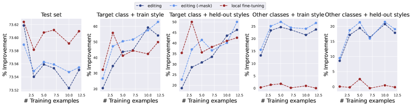
Figure 22: Editing vs. fine-tuning performance on an ImageNet-trained VGG16 classifier, as a function of the number of train exemplars. Here, we visualize the average number of misclassifications corrected over different concept-transformation pairs, with concepts derived from instance segmentation modules trained on MS-COCO; and transformations described in Appendix A.4.1. For both editing and fine-tuning, the overall drop in model accuracy is less than $0.25\%$.

Rank restriction. We evaluate the performance of editing when the weight update is not restricted to a rank-one modification. We find that this change significantly reduces the efficacy of editing on examples from both the target and non-target classes—cf. curves corresponding to ‘-proj’ in Appendix Figures 23-26. This suggests that the rank restriction is necessary to prevent the model from overfitting to the few exemplars used.

Mask. During editing, [BZS+20] focus on rewriting only the key-value pairs that correspond to the concept of interest. We find, however, that imposing the editing constraints on the entirety of the image leads to even better performance—cf. curves corresponding to ‘-mask’ in Appendix Figures 23-26. We hypothesize that this has a regularizing effect as it constrains the weights to preserve the original mapping between keys and values in regions that do not contain the concept.

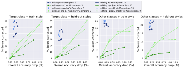
(a) Concepts derived from an instance segmentation model trained on MS-COCO.

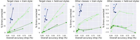
(b) Concepts derived from an instance segmentation model trained on LVIS.

Figure 23: Performance vs. drop in overall test set accuracy: Here, we visualize average number of misclassifications corrected by editing variants—based on whether or not we use a mask and perform a rank-one update—when applied to an ImageNet-trained VGG16 classifier.

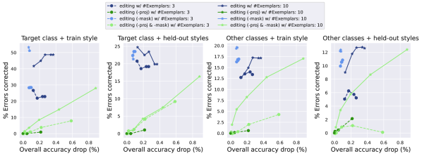
(a) Concepts derived from an instance segmentation model trained on MS-COCO.

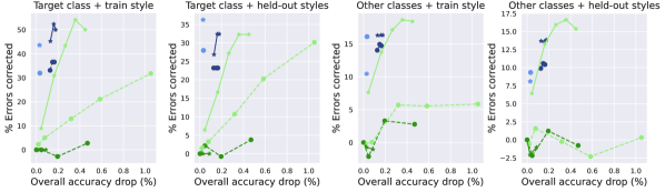
(b) Concepts derived from an instance segmentation model trained on LVIS.

Figure 24: Repeating the analysis in Appendix Fig. 23 on an ImageNet-trained ResNet-50 classifier.

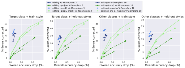
(a) Concepts derived from an instance segmentation model trained on MS-COCO.

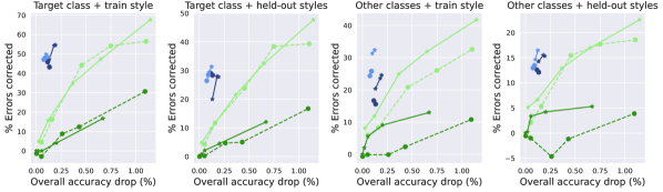
(b) Concepts derived from an instance segmentation model trained on LVIS.

Figure 25: Repeating the analysis in Appendix Fig. 23 on an Places365-trained VGG16 classifier.

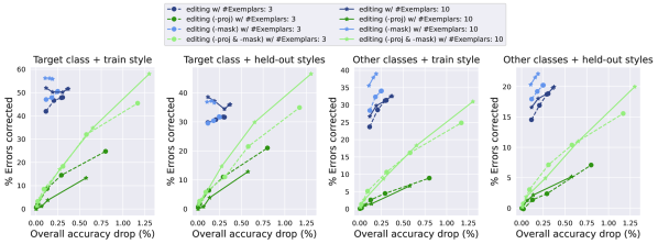
(a) Concepts derived from an instance segmentation model trained on MS-COCO.

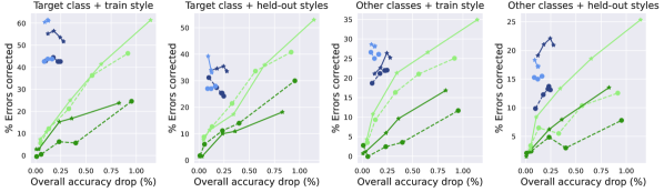
(b) Concepts derived from an instance segmentation model trained on LVIS.

Figure 26: Repeating the analysis in Appendix Fig. 23 on an Places365-trained ResNet-18 classifier.

B.2 Discovering Prediction-rules

Here, we expand on our analysis in Section 5 so as to characterize the effect of concept-level transformations on classifiers.

Per concept.

In Figure 27, we visualize the accuracy drop induced by transformations of a specific concept for classifiers trained on ImageNet and Places-365 (similar to Figure 6a). Here, the accuracy drop post-transformation is measured only on images that contain the concept of interest. We then present the average drop across transformations, along with 95% confidence intervals. We find that there is a large variance between: (i) a model’s reliance on different concepts, and (ii) different model’s reliance on a single concept. For instance, the accuracy of a ResNet-50 ImageNet classifier drops by more than 30% on the class “three-toed sloth” when “tree”s in the image are modified, while the accuracy of a VGG16 model drops by less than 5% under the same setup.

Per transformation.

In Figure 28, we illustrate how the model’s sensitivity to specific concepts varies depending on the applied transformation. Across concepts, we find that models are more sensitive to transformations to textures such as “grafitti” and “fall colors” than they are to “wooden” or “metallic”.

Per class (prediction-rules).

In Figure 29, we provide additional examples of class-level prediction rules identified using our methodology. Specifically, for each class, the highlighted concepts are those that hurt model accuracy when transformed.

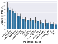
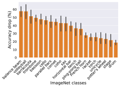
(a) Concept: “person”; Models: VGG16 (left) and ResNet-50 (right) trained on ImageNet-1k.

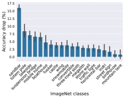
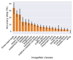
(b) Concept: “tree”; Models: VGG16 (left) and ResNet-50 (right) trained on ImageNet-1k.

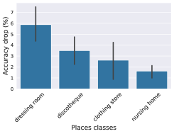
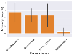
(c) Concept: “dress”; Models: VGG16 (left) and ResNet-18 (right) trained on Places-365.

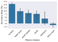
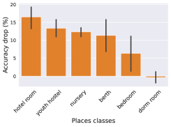
(d) Concept: “bed”; Models: VGG16 (left) and ResNet-18 (right) trained on Places-365.

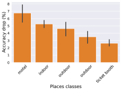
(e) Concept: “signboard”; Models: VGG16 (left) and ResNet-18 (right) trained on Places-365.

Figure 27: Dependence of a classifier on high-level concepts: average accuracy drop (along with 95% confidence intervals obtained via bootstrapping), over various styles, induced by the transformation of said concept. The classes for which the concept is most often present are shown.

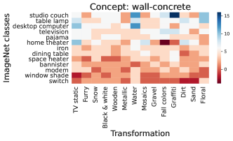
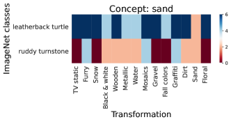
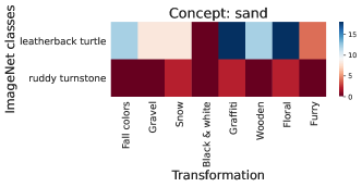
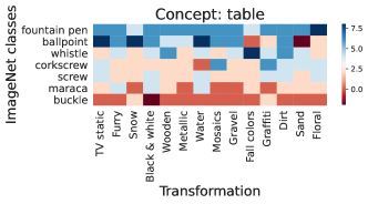
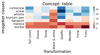
(a) VGG16 (left) and ResNet-50 (right) models trained on the ImageNet-1k dataset.

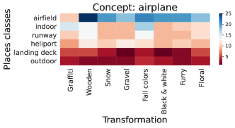
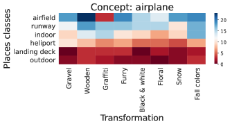
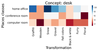
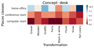
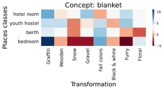
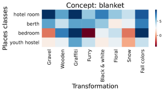
(b) VGG16 (left) and ResNet-18 (right) models trained on the Places-365 dataset.

Figure 28: Heatmaps illustrating classifier sensitivity to various concept-level transformations. Here, we measure model sensitivity in terms of the per class drop in model accuracy induced by the transformation on images of that class which contain the concept of interest.

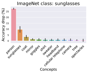
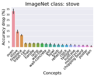
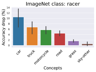
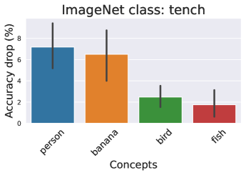
(a) VGG16 classifier trained on the ImageNet dataset.

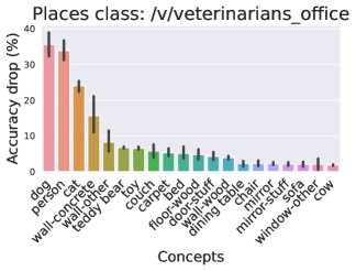
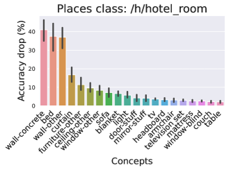
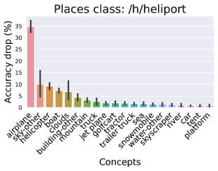
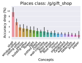
(b) ResNet-18 classifier trained on the Places-365 dataset.

Figure 29: Per-class prediction rules: high-level concepts, which when transformed, significantly hurt model performance on that class. Here, we visualize average accuracy drop (along with 95% confidence intervals obtained via bootstrapping) for a specific concept, over various styles.

References

- [ABG+19] Martin Arjovsky, Léon Bottou, Ishaan Gulrajani and David Lopez-Paz “Invariant risk minimization” In arXiv preprint arXiv:1907.02893, 2019
- [ASF20] Vedika Agarwal, Rakshith Shetty and Mario Fritz “Towards causal vqa: Revealing and reducing spurious correlations by invariant and covariant semantic editing” In Proceedings of the IEEE/CVF Conference on Computer Vision and Pattern Recognition, 2020, pp. 9690–9698
- [BBC+07] Shai Ben-David, John Blitzer, Koby Crammer and Fernando Pereira “Analysis of representations for domain adaptation” In Neural Information Processing Systems (NeurIPS), 2007
- [BHK+20] Lucas Beyer et al. “Are we done with ImageNet?” In arXiv preprint arXiv:2006.07159, 2020
- [BLW+20] David Bau et al. “Rewriting a deep generative model” In European Conference on Computer Vision (ECCV), 2020
- [BMA+19] Andrei Barbu et al. “ObjectNet: A large-scale bias-controlled dataset for pushing the limits of object recognition models” In Neural Information Processing Systems (NeurIPS), 2019
- [BS21] Collin Burns and Jacob Steinhardt “Limitations of Post-Hoc Feature Alignment for Robustness” In Computer Vision and Pattern Recognition (CVPR), 2021
- [BVA20] Alceu Bissoto, Eduardo Valle and Sandra Avila “Debiasing Skin Lesion Datasets and Models? Not So Fast” In Proceedings of the IEEE/CVF Conference on Computer Vision and Pattern Recognition Workshops, 2020, pp. 740–741
- [BVP18] Sara Beery, Grant Van Horn and Pietro Perona “Recognition in terra incognita” In European Conference on Computer Vision (ECCV), 2018
- [BZK+17] David Bau et al. “Network dissection: Quantifying interpretability of deep visual representations” In Computer Vision and Pattern Recognition (CVPR), 2017
- [BZS+19] David Bau et al. “GAN Dissection: Visualizing and Understanding Generative Adversarial Networks” In International Conference on Learning Representations (ICLR), 2019
- [BZS+20] David Bau et al. “Understanding the role of individual units in a deep neural network” In Proceedings of the National Academy of Sciences (PNAS), 2020
- [CBR20] Zhi Chen, Yijie Bei and Cynthia Rudin “Concept whitening for interpretable image recognition” In Nature Machine Intelligence, 2020
- [CFT+16] Nicolas Courty, Rémi Flamary, Devis Tuia and Alain Rakotomamonjy “Optimal transport for domain adaptation” In Transactions on Pattern Analysis and Machine Intelligence, 2016
- [CPK+17] Liang-Chieh Chen et al. “Deeplab: Semantic image segmentation with deep convolutional nets, atrous convolution, and fully connected crfs” In IEEE transactions on pattern analysis and machine intelligence, 2017
- [DAT21] Nicola De Cao, Wilker Aziz and Ivan Titov “Editing Factual Knowledge in Language Models” In arXiv preprint arXiv:2104.08164, 2021
- [DDH+21] Damai Dai et al. “Knowledge neurons in pretrained transformers” In arXiv preprint arXiv:2104.08696, 2021
- [DDS+09] Jia Deng et al. “Imagenet: A large-scale hierarchical image database” In Computer Vision and Pattern Recognition (CVPR), 2009
- [DJV+14] Jeff Donahue et al. “Decaf: A deep convolutional activation feature for generic visual recognition” In International conference on machine learning (ICML), 2014
- [EBC+09] Dumitru Erhan, Yoshua Bengio, Aaron Courville and Pascal Vincent “Visualizing higher-layer features of a deep network” In Technical Report, University of Montreal, 2009
- [EIS+19] Logan Engstrom et al. “Adversarial Robustness as a Prior for Learned Representations” In ArXiv preprint arXiv:1906.00945, 2019
- [ETT+19] Logan Engstrom et al. “Exploring the Landscape of Spatial Robustness” In International Conference on Machine Learning (ICML), 2019
- [FF15] Alhussein Fawzi and Pascal Frossard “Manitest: Are classifiers really invariant?” In British Machine Vision Conference (BMVC), 2015
- [FGC+19] Nic Ford, Justin Gilmer, Nicolas Carlini and Dogus Cubuk “Adversarial Examples Are a Natural Consequence of Test Error in Noise” In arXiv preprint arXiv:1901.10513, 2019
- [FMF16] Alhussein Fawzi, Seyed-Mohsen Moosavi-Dezfooli and Pascal Frossard “Robustness of classifiers: from adversarial to random noise” In Advances in Neural Information Processing Systems (NeurIPS), 2016
- [GAO+19] Lore Goetschalckx, Alex Andonian, Aude Oliva and Phillip Isola “Ganalyze: Toward visual definitions of cognitive image properties” In Proceedings of the IEEE/CVF International Conference on Computer Vision, 2019, pp. 5744–5753
- [GCV+21] Gabriel Goh et al. “Multimodal neurons in artificial neural networks” In Distill, 2021
- [GDG19] Agrim Gupta, Piotr Dollar and Ross Girshick “LVIS: A Dataset for Large Vocabulary Instance Segmentation” In Conference on Computer Vision and Pattern Recognition (CVPR), 2019
- [GEB16] Leon A Gatys, Alexander S Ecker and Matthias Bethge “Image style transfer using convolutional neural networks” In computer vision and pattern recognition (CVPR), 2016
- [GFS+19] Yash Goyal, Amir Feder, Uri Shalit and Been Kim “Explaining classifiers with causal concept effect (cace)” In arXiv preprint arXiv:1907.07165, 2019
- [GJM+20] Robert Geirhos et al. “Shortcut learning in deep neural networks” In Nature Machine Intelligence, 2020
- [GL15] Yaroslav Ganin and Victor Lempitsky “Unsupervised domain adaptation by backpropagation” In International Conference in Machine Learning (ICML), 2015
- [GLK+17] Golnaz Ghiasi et al. “Exploring the structure of a real-time, arbitrary neural artistic stylization network” In arXiv preprint arXiv:1705.06830, 2017
- [GRG+18] Ross Girshick et al. “Detectron”, https://github.com/facebookresearch/detectron, 2018
- [GWE+19] Yash Goyal et al. “Counterfactual visual explanations” In arXiv preprint arXiv:1904.07451, 2019
- [GZL+16] Mingming Gong et al. “Domain adaptation with conditional transferable components” In International conference on machine learning (ICML), 2016
- [HD19] Dan Hendrycks and Thomas G. Dietterich “Benchmarking Neural Network Robustness to Common Corruptions and Surface Variations” In International Conference on Learning Representations (ICLR), 2019
- [HHL+20] Erik Härkönen, Aaron Hertzmann, Jaakko Lehtinen and Sylvain Paris “GANSpace: Discovering Interpretable GAN Controls” In Advances in Neural Information Processing Systems 33, 2020
- [HM17] Christina Heinze-Deml and Nicolai Meinshausen “Conditional variance penalties and domain shift robustness” In arXiv preprint arXiv:1710.11469, 2017
- [HMC+19] Dan Hendrycks et al. “Augmix: A simple data processing method to improve robustness and uncertainty” In arXiv preprint arXiv:1912.02781, 2019
- [HZR+15] Kaiming He, Xiangyu Zhang, Shaoqing Ren and Jian Sun “Deep Residual Learning for Image Recognition” In Conference on Computer Vision and Pattern Recognition (CVPR), 2015
- [HZR+16] Kaiming He, Xiangyu Zhang, Shaoqing Ren and Jian Sun “Deep Residual Learning for Image Recognition” In Conference on Computer Vision and Pattern Recognition (CVPR), 2016
- [JCI19] Ali Jahanian, Lucy Chai and Phillip Isola “On the" steerability" of generative adversarial networks” In International Conference on Learning Representations, 2019
- [KHL19] Divyansh Kaushik, Eduard Hovy and Zachary Lipton “Learning The Difference That Makes A Difference With Counterfactually-Augmented Data” In International Conference on Learning Representations (ICLR), 2019
- [KML20] Ananya Kumar, Tengyu Ma and Percy Liang “Understanding Self-Training for Gradual Domain Adaptation” In International Conference on Machine Learning (ICML), 2020
- [KNT+20] Pang Wei Koh et al. “Concept bottleneck models” In International Conference on Machine Learning (ICML), 2020
- [KSH+19] Daniel Kang et al. “Testing Robustness Against Unforeseen Adversaries” In ArXiv preprint arxiv:1908.08016, 2019
- [KSM+20] Pang Wei Koh et al. “WILDS: A Benchmark of in-the-Wild Distribution Shifts” In arXiv preprint arXiv:2012.07421, 2020
- [KWG+18] Been Kim et al. “Interpretability beyond feature attribution: Quantitative testing with concept activation vectors (tcav)” In International conference on machine learning (ICML), 2018
- [KZM+12] Aditya Khosla et al. “Undoing the damage of dataset bias” In European Conference on Computer Vision (ECCV), 2012
- [LFS19] Max Losch, Mario Fritz and Bernt Schiele “Interpretability beyond classification output: Semantic bottleneck networks” In arXiv preprint arXiv:1907.10882, 2019
- [LMB+14] Tsung-Yi Lin et al. “Microsoft coco: Common objects in context” In European conference on computer vision (ECCV), 2014
- [LNH09] Christoph H Lampert, Hannes Nickisch and Stefan Harmeling “Learning to detect unseen object classes by between-class attribute transfer” In Computer Vision and Pattern Recognition (CVPR), 2009
- [LWS+16] Yanghao Li et al. “Revisiting batch normalization for practical domain adaptation” In arXiv preprint arXiv:1603.04779, 2016
- [LYP+19] Raphael Gontijo Lopes et al. “Improving robustness without sacrificing accuracy with patch gaussian augmentation” In arXiv preprint arXiv:1906.02611, 2019
- [MJI+17] Saeid Motiian, Quinn Jones, Seyed Mehdi Iranmanesh and Gianfranco Doretto “Few-Shot Adversarial Domain Adaptation” In NIPS, 2017
- [MLB+21] Eric Mitchell et al. “Fast Model Editing at Scale” In arXiv preprint arXiv:2110.11309, 2021
- [MMS+18] Aleksander Madry et al. “Towards deep learning models resistant to adversarial attacks” In International Conference on Learning Representations (ICLR), 2018
- [OMS17] Chris Olah, Alexander Mordvintsev and Ludwig Schubert “Feature Visualization” In Distill, 2017
- [OSH+19] Yonatan Oren, Shiori Sagawa, Tatsunori Hashimoto and Percy Liang “Distributionally Robust Language Modeling” In Empirical Methods in Natural Language Processing (EMNLP), 2019
- [OSJ+18] Chris Olah et al. “The Building Blocks of Interpretability” In Distill, 2018
- [PBE+06] Jean Ponce et al. “Dataset issues in object recognition” In Toward category-level object recognition, 2006
- [Pea10] Judea Pearl “Causal inference” In Causality: Objectives and Assessment PMLR, 2010
- [RDS+15] Olga Russakovsky et al. “ImageNet Large Scale Visual Recognition Challenge” In International Journal of Computer Vision (IJCV), 2015
- [RKH+21] Alec Radford et al. “Learning transferable visual models from natural language supervision” In arXiv preprint arXiv:2103.00020, 2021
- [RRS+19] Benjamin Recht, Rebecca Roelofs, Ludwig Schmidt and Vaishaal Shankar “Do ImageNet Classifiers Generalize to ImageNet?” In International Conference on Machine Learning (ICML), 2019
- [RSG16] Marco Tulio Ribeiro, Sameer Singh and Carlos Guestrin ““Why Should I Trust You?”: Explaining the Predictions of Any Classifier” In International Conference on Knowledge Discovery and Data Mining (KDD), 2016
- [RZT18] Amir Rosenfeld, Richard Zemel and John K. Tsotsos “The Elephant in the Room” In arXiv preprint arXiv:1808.03305, 2018
- [SAS+14] Ali Sharif Razavian, Hossein Azizpour, Josephine Sullivan and Stefan Carlsson “CNN features off-the-shelf: an astounding baseline for recognition” In conference on computer vision and pattern recognition (CVPR) workshops, 2014
- [SC18] Pierre Stock and Moustapha Cisse “Convnets and imagenet beyond accuracy: Understanding mistakes and uncovering biases” In European Conference on Computer Vision (ECCV), 2018
- [SFS18] Rakshith Shetty, Mario Fritz and Bernt Schiele “Adversarial Scene Editing: Automatic Object Removal from Weak Supervision” In NeurIPS, 2018
- [SGT+20] Yujun Shen, Jinjin Gu, Xiaoou Tang and Bolei Zhou “Interpreting the latent space of gans for semantic face editing” In Proceedings of the IEEE/CVF Conference on Computer Vision and Pattern Recognition, 2020, pp. 9243–9252
- [SKF+10] Kate Saenko, Brian Kulis, Mario Fritz and Trevor Darrell “Adapting visual category models to new domains” In European conference on computer vision (ECCV), 2010
- [SKH+20] Shiori Sagawa, Pang Wei Koh, Tatsunori B. Hashimoto and Percy Liang “Distributionally Robust Neural Networks for Group Shifts: On the Importance of Regularization for Worst-Case Generalization” In International Conference on Learning Representations, 2020
- [SSF19] Rakshith Shetty, Bernt Schiele and Mario Fritz “Not Using the Car to See the Sidewalk–Quantifying and Controlling the Effects of Context in Classification and Segmentation” In Proceedings of the IEEE/CVF Conference on Computer Vision and Pattern Recognition, 2019, pp. 8218–8226
- [STM21] Shibani Santurkar, Dimitris Tsipras and Aleksander Madry “Breeds: Benchmarks for subpopulation shift” In International Conference on Learning Representations (ICLR), 2021
- [SZ15] Karen Simonyan and Andrew Zisserman “Very Deep Convolutional Networks for Large-Scale Image Recognition” In International Conference on Learning Representations (ICLR), 2015
- [SZS+14] Christian Szegedy et al. “Intriguing properties of neural networks” In International Conference on Learning Representations (ICLR), 2014
- [TE11] Antonio Torralba and Alexei A Efros “Unbiased look at dataset bias” In CVPR 2011, 2011
- [TSE+20] Dimitris Tsipras et al. “From ImageNet to Image Classification: Contextualizing Progress on Benchmarks” In International Conference on Machine Learning (ICML), 2020
- [TT14] Tatiana Tommasi and Tinne Tuytelaars “A testbed for cross-dataset analysis” In European Conference on Computer Vision (ECCV), 2014
- [WLS20] Zongze Wu, Dani Lischinski and Eli Shechtman “StyleSpace Analysis: Disentangled Controls for StyleGAN Image Generation” In Computer Vision and Pattern Recognition (CVPR), 2020
- [WSM21] Eric Wong, Shibani Santurkar and Aleksander Madry “Leveraging Sparse Linear Layers for Debuggable Deep Networks” In International Conference on Machine Learning (ICML), 2021
- [XEI+20] Kai Xiao, Logan Engstrom, Andrew Ilyas and Aleksander Madry “Noise or signal: The role of image backgrounds in object recognition” In arXiv preprint arXiv:2006.09994, 2020
- [YLS+19] Dong Yin et al. “A fourier perspective on model robustness in computer vision” In Neural Information Processing Systems (NeurIPS), 2019
- [ZDK+21] Linjun Zhang et al. “How Does Mixup Help With Robustness and Generalization?” In International Conference on Learning Representations (ICLR), 2021
- [ZF14] Matthew D Zeiler and Rob Fergus “Visualizing and understanding convolutional networks”, 2014
- [ZLK+17] Bolei Zhou et al. “Places: A 10 million image database for scene recognition” In IEEE transactions on pattern analysis and machine intelligence, 2017
- [ZML+07] Jianguo Zhang, Marcin Marszałek, Svetlana Lazebnik and Cordelia Schmid “Local features and kernels for classification of texture and object categories: A comprehensive study” In International journal of computer vision, 2007
- [ZSB+18] Bolei Zhou, Yiyou Sun, David Bau and Antonio Torralba “Interpretable basis decomposition for visual explanation” In Proceedings of the European Conference on Computer Vision (ECCV), 2018, pp. 119–134