Gaussian Mixture Variational Autoencoder with Contrastive Learning
for Multi-Label Classification

Abstract

Multi-label classification (MLC) is a prediction task where each sample can have more than one label. We propose a novel contrastive learning boosted multi-label prediction model based on a Gaussian mixture variational autoencoder (C-GMVAE), which learns a multimodal prior space and employs a contrastive loss. Many existing methods introduce extra complex neural modules like graph neural networks to capture the label correlations, in addition to the prediction modules. We find that by using contrastive learning in the supervised setting, we can exploit label information effectively in a data-driven manner, and learn meaningful feature and label embeddings which capture the label correlations and enhance the predictive power. Our method also adopts the idea of learning and aligning latent spaces for both features and labels. In contrast to previous works based on a unimodal prior, C-GMVAE imposes a Gaussian mixture structure on the latent space, to alleviate the posterior collapse and over-regularization issues. C-GMVAE outperforms existing methods on multiple public datasets and can often match other models’ full performance with only 50% of the training data. Furthermore, we show that the learnt embeddings provide insights into the interpretation of label-label interactions.

1 Introduction

In many machine learning tasks, an instance can have several labels. The task of predicting multiple labels is known as multi-label classification (MLC). MLC is common in domains like computer vision (Wang et al., 2016), natural language processing (Chang et al., 2019) and biology (Yu et al., 2013). Unlike the single-label scenario, label correlations are more important in MLC. Early works capture the correlations through classifier chains (Read et al., 2009), Bayesian inference (Zhang & Zhou, 2007), and dimensionality reduction (Bhatia et al., 2015).

Thanks to the huge capacity of neural networks (NN), many previous methods can be improved by their neural extensions. For example, classifier chains can be naturally enhanced by recurrent neural networks (RNN) (Wang et al., 2016). The non-linearity of NN alleviates the complex design of feature mapping and many deep models can therefore focus on the loss function, feature-label and label-label correlation modeling.

One trending direction is to learn a deep latent space shared by features and labels. The encoded samples from the latent space are then decoded to targets. One typical example is C2AE (Yeh et al., 2017), which learns latent codes for both features and labels. The latent codes are passed to a decoder to derive the target labels. C2AE minimizes an $\ell_{2}$ distance between the feature and label codes, together with a relaxed orthogonality regularization. However, the learnt deterministic latent space lacks smoothness and structures. Small perturbations in this latent space can lead to totally different decoding results. Even if the corresponding feature and label codes are close, we cannot guarantee the decoded targets are similar. To address this concern, MPVAE (Bai et al., 2020) proposes to replace the deterministic latent space with a probabilistic space under a variational autoencoder (VAE) framework. The Gaussian latent spaces are aligned with KL-divergence, and the sampling process enforces smoothness. Similar ideas can be found in (Sundar et al., 2020). However, these methods assume a unimodal Gaussian latent space, which is known to cause over-regularization and posterior collapse (Dilokthanakul et al., 2016; Wu & Goodman, 2018). A better strategy would be to learn a multimodal latent space. It is more reasonable to assume the observed data are generated from a multimodal subspace rather than a unimodal one.

Another popular group of methods focuses on better label correlation modeling. Their idea is straightforward: some labels should be more correlated if they co-appear often while others should be less relevant. Existing methods adopt pairwise ranking loss, covariance matrices, conditional random fields (CRF) or graph neural nets (GNN) to this end (Zhang & Zhou, 2013; Bi & Kwok, 2014; Belanger & McCallum, 2016; Lanchantin et al., 2019; Chen et al., 2019b). These methods often either constrain the learning through a predefined structure (which requires a larger model size), or aren’t powerful enough to capture the correlations (such as pairwise ranking loss).

Our idea is simple: we learn embeddings for each label class and the inner products between embeddings should reflect the similarity. We further learn feature embeddings whose inner products with label embeddings correspond to feature-label similarity and can be used for prediction. We assume these embeddings are generated from a probabilistic multimodal latent space shared by features and labels, where we use KL-divergence to align the feature and label latent distributions. On the other hand, one might be concerned that embeddings alone won’t capture both label-label and label-feature correlations, which were usually modeled by extra GNN and covariance matrices in prior works (Lanchantin et al., 2019; Bai et al., 2020). To this end, we stress on the loss function terms rather than extra structure to capture these correlations. Intuitively, if two labels co-appear often, their embeddings should be close. Otherwise, if two labels seldom co-appear, their embeddings should be distant. A triplet-like loss could be naturally applied in this scenario. Nonetheless, its extension, contrastive loss, has shown to be even more effective than the triplet loss by introducing more samples rather than just one triplet. We show that contrastive loss can pull together correlated label embeddings, push away unrelated label embeddings (see Fig. 3), and even perform better than GNN-based or covariance-based methods.

Our new model for MLC, contrastive learning boosted Gaussian mixture variational autoencoder (C-GMVAE), alleviates the over-regularization and posterior collapse concerns, and also learns useful feature and label embeddings. C-GMVAE is applied to nine datasets and outperforms the existing methods on five metrics. Moreover, we show that using only 50% of the data, our results can match the full performance of other state-of-the-art methods. Ablation studies and interpretability of learnt embeddings will also be illustrated in the experiments. Our contributions can be summarized in three aspects: (i) We propose to use contrastive loss instead of triplet or ranking loss to strengthen the label embedding learning. We empirically show that by using a contrastive loss, one can get rid of heavy-duty label correlation modules (e.g., covariance matrices, GNNs) while achieving even better performances. (ii) Though contrastive learning is commonly applied in self-supervised learning, our work shows that by properly defining anchor, positive and negative samples, contrastive loss can leverage label information very effectively in the supervised MLC scenario as well. (iii) Unlike prior probabilistic models, C-GMVAE learns a multimodal latent space and integrates the probabilistic modeling (VAE module) with embedding learning (contrastive module) synergistically.

2 Methods

In MLC, given a dataset containing $N$ labeled samples $(x,y)$, where $x\in\mathbb{R}^{D}$ and $y\in\mathbb{\{}0,1\}^{L}$, our goal is to find a mapping from $x$ to $y$. $N,D,L$ are the number of samples, feature length and label set size respectively. The binary coding indicates the labels associated with the sample $x$. Labels are correlated with each other.

2.1 Preliminaries

2.1.1 Gaussian Mixture VAE

A standard VAE (Kingma & Welling, 2013) pulls together the posterior distribution and a parameter-free isotropic Gaussian prior. Two losses are optimized together in training: KL-divergence from the prior to the posterior, and the distance between the reconstructed targets and the real targets. One weakness of this formulation is the unimodality of its latent space, inhibiting the learning of more complex representations. Another concern is over-regularization: if the posterior is exactly the same as the prior, the learnt representations would be uninformative of the inputs. Numerous works extend the prior to be more complex (Chung et al., 2015; Eslami et al., 2016; Dilokthanakul et al., 2016). In our work, we adopt the Gausian mixture prior. The probability density can be depicted as $p(z)=\frac{1}{k}\sum_{i=1}^{k}\mathcal{N}(z|\mu_{i},\sigma_{i}^{2})$ where $i$ is the cluster index of $k$ Gaussian clusters with mean $\mu_{i}$ and covariance $\sigma_{i}^{2}$ (Shu, 2016; Shi et al., 2019). Our intuition is that each label embedding could correlate to a Gaussian subspace. Given a label set, the mixture of the positive Gaussian subspaces forms a unique multimodal prior distribution. The label embeddings also receive the gradients from the contrastive loss and thus the contrastive learning is combined with latent space construction. Our formulation is also related to MVAE (Wu & Goodman, 2018; Shi et al., 2020) which adopts the idea of product-of-experts.

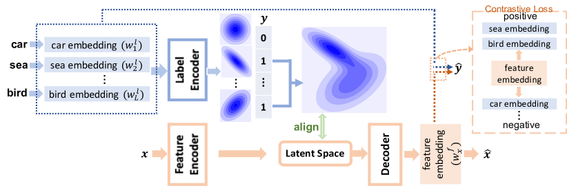
Figure 1: The full pipeline of C-GMVAE. Every label category is mapped to a learnable embedding first. The label encoder transforms each embedding $w_{i}^{l}$ to a multivariate Gaussian latent space. The sample’s associated label set selects the positive latent spaces and forms a Gaussian mixture prior. Each feature is also mapped to a latent space through a feature encoder. The posterior is aligned with the prior via KL-divergence. The decoder takes in a sample from the latent space and produces a feature embedding $w_{x}^{f}$. A contrastive loss is designed to pull together the feature embedding and the positive label embeddings, while separating the feature embedding from the negative label embeddings. Prediction $\hat{y}$ is generated by passing the inner products between the feature embedding $w_{x}^{f}$ and the label embeddings $w_{i}^{l}$ to the sigmoid functions. A sample with label set {sea, bird} is shown here.

2.1.2 Contrastive Learning

We propose to use contrastive learning to capture the correlations (i.e., feature-label and label-label correlations). Contrastive learning (Oord et al., 2018; Chen et al., 2020; Khosla et al., 2021) is a novel learning style. The core idea is simple: given an anchor sample, it should be close to similar samples (positive) and far from dissimilar samples (negative) in some learnt embedding space. It differs from triplet loss in the number of negative samples and the loss estimation method. Contrastive loss is largely motivated by noise contrastive estimation (NCE) (Gutmann & Hyvärinen, 2010) and its form is generalizable. The raw contrastive loss formulation only considers the instance-level invariance (multiple views of one instance), but with label information, we can learn category-level invariance (multiple instances per class/category) (Wang et al., 2021).

In the multi-label scenario, one can regard the feature embedding as the anchor sample, positive label embeddings as the positive samples and negative label embeddings as the negative samples. The formulation can fit the contrastive learning framework naturally and is one of our major contributions. Compared to the pairwise ranking loss which focuses on the final logits, contrastive loss is defined on the learnt embeddings and thus becomes more expressive. Contrastive loss also includes more samples in estimating the NCE and therefore outperforms the triplet loss. In the appendix, we show triplet loss is actually a special case of our contrastive loss.

2.2 C-GMVAE

C-GMVAE inherits the general VAE framework, but with a learnable Gaussian mixture (GM) prior. During training, each sample’s label set activates and mixes the positive Gaussian subspaces to derive the prior. Contrastive learning is applied to boost the embedding learning, using a contrastive loss between the feature and label embeddings. Fig. 1 provides a full illustration, and the following subsections will elaborate on the details.

2.2.1 Gaussian Mixture Latent Space

Given a sample $(x,y)$ where feature $x\in\mathbb{R}^{D}$ and label $y\in\{0,1\}^{L}$, many previous works take $y$ as the input and transform it to a dense representation through a fully-connected layer (Yeh et al., 2017; Bai et al., 2020). This layer essentially maps each label category to an embedding and sums up all the embeddings using label $y$ as weights (0 or 1). The summed embedding is fed into the label encoder to produce a probabilistic latent space.

In C-GMVAE, however, we directly map each label embedding $w_{i}^{l}\in\mathbb{R}^{E}$ of label class $i$ to an individual latent Gaussian distribution $\mathcal{N}(\mu_{i},diag(\sigma_{i}^{2}))$, where $\mu_{i}\in\mathbb{R}^{d},\sigma_{i}^{2}\in\mathbb{R}^{d}$, and $\mu_{i},\sigma_{i}^{2}$ are derived from $w_{i}^{l}$ through the NN-based label encoder. The randomly initialized embeddings $w_{i}^{l}$ are learnable during the training process, similar to (Mikolov et al., 2013), and they share the same label encoder. In Fig. 1, the label categories car, sea,…, bird are transformed to embeddings first. Embeddings are then passed directly to label encoder rather than summed up. Each label category (e.g., car) corresponds to a unimodal Gaussian in the latent space. $y$ activates “positive” Gaussians ($y_{i}=1$) and forms a Gaussian mixture subspace. Given a random variable $z\in\mathbb{R}^{d}$, the probability density function (PDF) in the subspace is defined as

$$p_{\psi}(z|y)=\frac{1}{\sum_{i}y_{i}}\sum_{i=1}^{L}\mathbbm{1}\{y_{i}=1\}\mathcal{N}(z|\mu_{i},diag(\sigma_{i}^{2}))$$ (1)

where $\mathbbm{1}(\cdot)$ is the indicator function and the label encoder is parameterized by $\psi$ (NN). In Fig. 1, $y$ activates sea and bird, then we have

$$p_{\psi}(z|y)=\frac{1}{2}( \mathcal{N}(z|\mu_{sea},diag(\sigma_{sea}^{2}))+$$ (2)

$$\mathcal{N}(z|\mu_{bird},diag(\sigma_{bird}^{2})))$$

Most VAE-based frameworks optimize over an evidence lower bound (ELBO) (Doersch, 2016):

$$\text{ELBO}=\mathbb{E}_{q_{\phi}(z|x)}[ \log p_{\theta}(x|z)]-$$ (3)

$$D_{KL}[q_{\phi}(z|x)||p(z)]$$

The feature encoder is parameterized by $\phi$ (NN). One pitfall of this objective is owing to the minimization of the KL-divergence. If the divergence between the posterior $q_{\phi}(z|x)$ and the prior $p_{\psi}(z)$ vanishes, the learnt latent codes would become non-informative. This is called posterior collapse. Many recent works suggest learnable priors (Tomczak & Welling, 2018) or more sophisticated priors (Wang & Wang, 2019) to avoid this issue, and we adopt these ideas in our design of the prior. Compared to a standard VAE, our prior is informative, learnable and multimodal.

We form a standard posterior in our model and match it with the prior. However, unlike vanilla VAE, we cannot analytically compute the KL term. Instead, we use the following estimation:

$$\mathcal{L}_{KL}\approx \log q_{\phi}(z_{0}|x)-\log p_{\psi}(z_{0}|y)$$ (4)

$$= \log\mathcal{N}(z_{0}|\mu_{\phi}(x),diag(\sigma_{\phi}^{2}(x)))-$$

$$\log\frac{1}{\sum_{i}y_{i}}\sum_{i=1}^{L}\mathbbm{1}\{y_{i}=1\}\mathcal{N}(z_{0}|\mu_{i},diag(\sigma_{i}^{2}))$$

where $z_{0}\sim q_{\phi}(z|x)$ denotes a single latent sample. Our formulation follows the design of (Shu, 2016), which has been shown to outperform the formulation in (Dilokthanakul et al., 2016).

The reconstruction loss is a standard negative log-likelihood with decoder parameters $\theta$,

$$\mathcal{L}_{recon}= -E_{q_{\phi}(z|x)}[\log p_{\theta}(x|z)]$$ (5)

2.2.2 Contrastive Learning Module

The decoder function $f_{\theta}^{d}(\cdot)$ decodes the sample from the latent space to a feature embedding $w^{f}_{x}\in\mathbb{R}^{E}$. We learn $w^{f}_{x}$ together with label embeddings $\{w_{i}^{l}\}_{i=1}^{L}$. The objective function includes both contrastive loss and cross-entropy loss terms.

Prior works explicitly capture the label-label interactions with GNNs or covariance matrices, which impose the structure a priori and might not be the best modeling approach. Our contrastive module instead captures the correlations in a data-driven manner. For example, if in most of the samples, “beach” and “sunshine” appear together, the contrastive learning will implicitly pull their embeddings together (see the derivation in the appendix). In other words, if two labels do co-appear often, their label embeddings would become similar (Fig. 3). On the other hand, if they never co-occur or only co-appear occasionally, their connections are not significant and our model will not optimize for their similarity.

Original contrastive learning (Oord et al., 2018) augments inputs and learns the instance-level invariance, but it may not generalize to the category-level invariance. In the supervised setting, however, the learning can benefit from the labels and discover the category-level invariance (Khosla et al., 2021). Let $A\equiv\{1...L\}$. We define $P(y)\equiv\{i\in A:y_{i}=1\}$ for sample $(x,y)$. Suppose we have a batch of samples, $\mathcal{B}$, the contrastive loss can be written as

$$\mathcal{L}_{CL}=\frac{1}{|\mathcal{B}|}\sum_{(x,y)\in\mathcal{B}}\frac{1}{|P(y)|}\sum_{p\in P(y)}-\log\frac{\text{sim}(w^{f}_{x},w_{p}^{l})}{\sum_{t\in A}\text{sim}(w^{f}_{x},w_{t}^{l})}$$ (6)

Here, $\text{sim}(\cdot)$ is a function measuring the similarity between two embeddings, and $w_{x}^{f}$, $w_{i}^{l}$ denote the feature and label embeddings respectively. Eq. 6 is built on top of NCE (Gutmann & Hyvärinen, 2010), and the equation is equivalent to a categorical cross-entropy of correctly predicting positive labels. The choice of $\text{sim}(\cdot)$ can be a log-bilinear function (Oord et al., 2018), or a more complicated neural metric function (Chen et al., 2020). In our experiments, we find it is simple and effective to take $\text{sim}(w_{1},w_{2})=\exp(w_{1}\cdot w_{2}/\tau)$ where $\cdot$ means inner product and $\tau$ is a temperature parameter controlling the scale of the inner product.

In the single-label scenarios like SupCon (Khosla et al., 2021), if one class is positive, all other classes are contrastive to it. However, in MLC, if “beach” is positive in the label set while “sea” is not for one particular sample, we cannot say these two classes are contrastive. Their correlations should be captured implicitly by all the samples. Therefore, we do not enforce contrastive relations between labels and thus preserve the label correlations. Instead, we choose the feature embedding to be the anchor and label embeddings to be the positive and negative samples. If two label embeddings co-appear often as positive samples, they would implicitly become similar (see Fig. 3). Eq. 6 saves the effort of manually configuring the positive and negative samples, and is totally data-driven. The number of positive or negative samples could be greater than one, depending on the label set. Though $L$ limits the max samples we can have, this formulation has already used many more samples compared to triplet loss, and we will show in experiments that this formulation is very effective.

The triplet loss often used in multi-label learning (Seymour & Zhang, 2018) can be seen as a special case of Eq. 6 with only one positive and one negative. We illustrate this connection in the appendix. Furthermore, one desired property of embedding learning is that when a good positive embedding is already close enough to our anchor embedding, it contributes less to the gradients, while poorly learnt embeddings contribute more to improve the model performance. In the appendix, we also show that the contrastive loss can implicitly achieve this goal and a full derivation of the gradients is provided.

Our objective function also includes a supervised cross-entropy loss term to further facilitate the training. With the label embeddings $w_{i}^{l}$ and the feature embedding $w_{x}^{f}$, the cross entropy loss for each $(x,y)$ is given by

$$\mathcal{L}_{CE}=\sum_{i=1}^{L}y_{i}\log s(w_{x}^{f}w_{i}^{l})+(1-y_{i})\log(1-s(w_{x}^{f}w_{i}^{l}))$$ (7)

where $s(\cdot)$ is the sigmoid function. In self-supervised learning, the contrastive loss typically helps the pretraining stage and the learnt representations are applied to downstream tasks. In the supervised setting, though some models (Khosla et al., 2021) stick to the two-stage training process where the model is trained with contrastive loss in the first stage and with cross-entropy loss in the second stage, we did not observe its superiority over the one-stage scheme in our MLC scenario. This is partly because we also learn a latent space that is closely connected to label embeddings. We train the model with an objective function incorporating all the losses. A joint training strategy reconciles different modules. We show in the experiments that the learnt embeddings are semantically meaningful and can reveal the label correlations.

2.2.3 Objective Function

The final objective function to minimize is simply the summation of different losses,

$$\mathcal{L}=\mathcal{L}_{KL}+\mathcal{L}_{recon}+\alpha\mathcal{L}_{CL}-\beta\mathcal{L}_{CE}$$ (8)

where $\alpha,\beta$ are trade-off weights. The model is trained with Adam (Kingma & Ba, 2014). Our model is optimized with $\mathcal{L}$ and will be tested on five different metrics. This is different from the methods that only optimize and test for specific metrics (Koyejo et al., 2015; Decubber et al., 2018).

2.3 Prediction

During the testing phase, the input sample $x$ will be passed to the feature encoder and decoder to obtain its embedding $w_{x}^{f}$. Label embeddings $w_{i}^{l}$ are fixed in testing. The inner products between $w_{x}^{f}$ and $w_{i}^{l}$ will be passed through a sigmoid function to obtain the prediction probability for each class $i$.

2.4 Insights behind C-GMVAE

C2AE and MPVAE have shown the importance of learning a shared latent space for both features and labels. These methods share the same high-level insight similar to a teacher-student regime: we map labels (teacher) to a latent space with some certain structure, which preserves the label information and is easier to decode back to labels. Then the features (student) are expected to be mapped to this latent space to facilitate the label prediction. Two general concerns exist for these methods: 1) the unimodal Gaussian space previously used is too restrictive to impose sophisticated structures on prior, and 2) they do not properly capture label correlations with embeddings. To address the first, we learn a modality for each label class to form a mixture latent space. For the second, we replace the commonly used ranking and triplet losses with contrastive loss since contrastive loss involves more samples than triplet loss and has a larger capacity than ranking loss.

Metric	example-F1									micro-F1
Dataset	eBird	mirflickr	nus-vec	yeast	scene	sider	reuters	bkms	delicious	eBird	mirflickr	nus-vec	yeast	scene	sider	reuters	bkms	delicious
BR	0.365	0.325	0.343	0.630	0.606	0.766	0.733	0.171	0.174	0.384	0.371	0.371	0.655	0.706	0.796	0.767	0.125	0.197
MLKNN	0.510	0.383	0.342	0.618	0.691	0.738	0.703	0.213	0.259	0.557	0.415	0.368	0.625	0.667	0.772	0.680	0.181	0.264
HARAM	0.510	0.432	0.396	0.629	0.717	0.722	0.711	0.216	0.267	0.573	0.447	0.415	0.635	0.693	0.754	0.695	0.230	0.273
SLEEC	0.258	0.416	0.431	0.643	0.718	0.581	0.885	0.363	0.308	0.412	0.413	0.428	0.653	0.699	0.697	0.845	0.300	0.333
C2AE	0.501	0.501	0.435	0.614	0.698	0.768	0.818	0.309	0.326	0.546	0.545	0.472	0.626	0.713	0.798	0.799	0.316	0.348
LaMP	0.477	0.492	0.376	0.624	0.728	0.766	0.906	0.389	0.372	0.517	0.535	0.472	0.641	0.716	0.797	0.886	0.373	0.386
MPVAE	0.551	0.514	0.468	0.648	0.751	0.769	0.893	0.382	0.373	0.593	0.552	0.492	0.655	0.742	0.800	0.881	0.375	0.393
ASL	0.528	0.477	0.468	0.613	0.770	0.752	0.880	0.373	0.359	0.580	0.525	0.495	0.637	0.753	0.795	0.869	0.354	0.387
RBCC	0.503	0.468	0.466	0.605	0.758	0.733	0.857	-	-	0.558	0.513	0.490	0.623	0.749	0.784	0.825	-	-
C-GMVAE	0.576	0.534	0.481	0.656	0.777	0.771	0.917	0.392	0.381	0.633	0.575	0.510	0.665	0.762	0.803	0.890	0.377	0.403
std ($\pm$)	0.001	0.002	0.000	0.001	0.002	0.001	0.001	0.001	0.002	0.001	0.001	0.000	0.002	0.002	0.000	0.001	0.001	0.002

Table 1: The example-F1 (ex-F1) and micro-F1 (mi-F1) scores of different methods on all datasets. C-GMVAE’s numbers are averaged over 3 seeds. The standard deviation (std) is also shown. 0.000 means an std$<0.0005$.

Metric	macro-F1									Hamming Accuracy
Dataset	eBird	mirflickr	nus-vec	yeast	scene	sider	reuters	bkms	delicious	eBird	mirflickr	nus-vec	yeast	scene	sider	reuters	bkms	delicious
BR	0.116	0.182	0.083	0.373	0.704	0.588	0.137	0.038	0.066	0.816	0.886	0.971	0.782	0.901	0.747	0.994	0.990	0.982
MLKNN	0.338	0.266	0.086	0.472	0.693	0.667	0.066	0.041	0.053	0.827	0.877	0.971	0.784	0.863	0.715	0.992	0.991	0.981
HARAM	0.474	0.284	0.157	0.448	0.713	0.649	0.100	0.140	0.074	0.819	0.634	0.971	0.744	0.902	0.650	0.905	0.990	0.981
SLEEC	0.363	0.364	0.135	0.425	0.699	0.592	0.403	0.195	0.142	0.816	0.870	0.971	0.782	0.894	0.675	0.996	0.989	0.982
C2AE	0.426	0.393	0.174	0.427	0.728	0.667	0.363	0.232	0.102	0.771	0.897	0.973	0.764	0.893	0.749	0.995	0.991	0.981
LaMP	0.381	0.387	0.203	0.480	0.745	0.668	0.520	0.286	0.196	0.811	0.897	0.980	0.786	0.903	0.751	0.997	0.992	0.982
MPVAE	0.494	0.422	0.211	0.482	0.750	0.690	0.545	0.285	0.181	0.829	0.898	0.980	0.792	0.909	0.755	0.997	0.991	0.982
ASL	0.467	0.410	0.208	0.484	0.765	0.668	0.563	0.264	0.183	0.831	0.893	0.975	0.796	0.912	0.759	0.997	0.991	0.982
RBCC	0.443	0.409	0.202	0.480	0.753	0.654	0.503	-	-	0.815	0.888	0.975	0.793	0.904	0.753	0.997	-	-
C-GMVAE	0.538	0.440	0.226	0.487	0.769	0.691	0.582	0.291	0.197	0.847	0.903	0.984	0.796	0.915	0.767	0.997	0.992	0.983
std ($\pm$)	0.000	0.001	0.001	0.002	0.002	0.002	0.001	0.001	0.001	0.001	0.000	0.000	0.002	0.001	0.003	0.000	0.000	0.000

Table 2: The macro-F1 (ma-F1) and Hamming accuracy (HA) scores of different methods on all datasets. C-GMVAE’s numbers are averaged over 3 seeds.

Dataset	eBird	mir.	nus-vec	yeast	scene	sider	reuters	bkms	del.
BR	0.598	0.582	0.443	0.745	0.700	0.573	0.752	0.301	0.485
MLKNN	0.772	0.491	0.456	0.730	0.675	0.916	0.753	0.310	0.460
MLARAM	0.768	0.350	0.404	0.682	0.722	0.930	0.679	0.312	0.419
SLEEC	0.656	0.623	0.531	0.745	0.730	0.882	0.908	0.415	0.676
C2AE	0.753	0.705	0.569	0.749	0.703	0.923	0.845	0.407	0.609
LaMP	0.737	0.685	0.456	0.740	0.746	0.937	0.927	0.420	0.663
MPVAE	0.820	0.726	0.587	0.743	0.777	0.958	0.930	0.437	0.696
ASL	0.818	0.681	0.586	0.752	0.770	0.954	0.929	0.418	0.692
RBCC	0.805	0.682	0.582	0.745	0.777	0.942	0.913	-	-
C-GMVAE	0.825	0.732	0.595	0.751	0.788	0.962	0.939	0.465	0.707

Table 3: The precision@1 scores of different methods on all datasets. “mir.” stands for mirflickr and “del.” means delicious dataset.

3 Related Work

Learning a shared latent space for features and labels is a common and useful idea. For single-label prediction tasks, CADA-VAE (Schönfeld et al., 2019) learns and aligns latent label and feature spaces through distribution alignment losses. Similar ideas can be seen in out-of-distribution detection as well (Sundar et al., 2020). In multi-label scenarios, methods adopting this idea typically have a similar module that directly maps the multi-hot labels to embeddings (Yeh et al., 2017; Chen et al., 2019a; Bai et al., 2020). This is a rather difficult learning task. Suppose we have 30 label categories. There could be up to $2^{30}$ label sets. For probabilistic models like MPVAE, that means one latent label space has to represent up to $2^{30}$ label combinations. In contrast, C-GMVAE learns per-category subspaces and forms a mixture prior distribution based on the observed samples’ label sets.

Contrastive learning has become one of the most popular self-supervised learning techniques. It has also been applied to supervised learning tasks. SupCon (Khosla et al., 2021) first demonstrated the effectiveness of supervised contrastive loss in image classification tasks. It was soon generalized to other domains like visual reasoning (Małkiński & Mańdziuk, 2020; Dao et al., 2021). Nevertheless, these methods depend on vision-specific augmentation techniques and attention mechanisms. Another related work is multi-label contrastive learning (Song & Ermon, 2020). But the work does not deal with MLC. Instead, it extends contrastive learning to the identification of more than one positive sample, which resembles a multi-label scenario.

Some earlier works also attempted metric learning or triplet loss in MLC (Annarumma & Montana, 2017). Triplet loss typically only takes one pair of positive and negative samples for one anchor, while contrastive loss uses many more negative and positive samples. Recent papers found that more samples can greatly boost performance (Chen et al., 2020; Wang et al., 2021). Though our contrastive module is constrained by the maximum number of label classes, the number of used samples has already surpassed other losses (e.g., triplet loss), and our observations reinforce that more samples help with the performance.

4 Experiments

Dataset	# Samples	# Labels	Mean Labels /Sample	Median Labels /Sample	Max Labels /Sample	Mean Samples /Label
eBird	41778	100	20.69	18	96	8322.95
bookmarks	87856	208	2.03	1	44	584.67
nus-vec	269648	85	1.86	1	12	3721.7
mirflickr	25000	38	4.80	5	17	1247.34
reuters	10789	90	1.23	1	15	106.50
scene	2407	6	1.07	1	3	170.83
sider	1427	27	15.3	16	26	731.07
yeast	2417	14	4.24	4	11	363.14
delicious	16105	983	19.06	20	25	250.15

Table 4: Dataset Statistics.

	variations	eb-F1	mi-F1	ma-F1
ebird	uni-Gaussian	0.545	0.583	0.490
	GM only	0.561	0.603	0.511
	contrastive only	0.558	0.594	0.515
	GM+contrastive	0.576	0.633	0.538
mirflickr	uni-Gaussian	0.510	0.541	0.413
	GM only	0.521	0.561	0.429
	contrastive only	0.526	0.565	0.428
	GM+contrastive	0.534	0.575	0.440
nus-vec	uni-Gaussian	0.461	0.479	0.203
	GM only	0.472	0.505	0.218
	contrastive only	0.470	0.501	0.213
	GM+contrastive	0.481	0.510	0.226

Table 5: Ablation study on the contrastive learning module and the Gaussian mixture module. Note that both modules are contributions of this work. As shown in the table, GM consistently improves performance. The contrastive module can also further boost the performance.

	method (data %)	HA	ex-F1	mi-F1	ma-F1
ebird	MPVAE (100%)	0.829	0.551	0.593	0.494
	C-GMVAE (50%)	0.842	0.557	0.615	0.521
mirflickr	MPVAE (100%)	0.898	0.514	0.552	0.422
	C-GMVAE (50%)	0.899	0.512	0.553	0.412
nus-vec	MPVAE (100%)	0.980	0.468	0.492	0.211
	C-GMVAE (50%)	0.975	0.465	0.494	0.201

Table 6: Comparisons between MPVAE and C-GMVAE using 100% and 50% respectively.

module in C-GMVAE	eBird	mirflickr	nus-vec	yeast	scene	sider
Covariance	0.601	0.556	0.488	0.650	0.751	0.787
GNN	0.599	0.560	0.491	0.655	0.749	0.801
contrastive	0.633	0.575	0.510	0.665	0.762	0.803

Table 7: mi-F1 performance after replacing our contrastive module with a GNN or a covariance matrix.

We have various setups to validate the performance of C-GMVAE. First, we compare the example-F1, micro-F1 and macro-F1 scores, Hamming accuracies and precision@1 of different methods. Second, we compare their performance when fewer training data are available. Third, an ablation study shows the importance of the proposed modules. Finally, we demonstrate the interpretability of the label embeddings on the eBird dataset. Our code is publicly available.

4.1 Setup

For the main evaluation experiments, we use nine datasets, including image datasets mirflickr, nuswide, scene (Huiskes & Lew, 2008; Chua et al., 2009; Boutell et al., 2004), biology datasets sider, yeast (Kuhn et al., 2016; Nakai & Kanehisa, 1992), ecology dataset eBird (Fink et al., 2017), and text datasets reuters, bookmarks, delicious (Debole & Sebastiani, 2005; Katakis et al., 2008; Tsoumakas et al., 2008) (see Tab. 4 for dataset statistics). All features are collected in vector format (Lanchantin et al., 2019; Bai et al., 2020). The feature pre-processing is standard following previous works (Lanchantin et al., 2019; Bai et al., 2020) and the datasets are public. Each dataset is separated into training (80%), validation (10%) and testing (10%) splits. The datasets are also preprocessed to fit the input formats of different methods. We use mini-batch training with batch size 128. Each batch is randomly sampled from the dataset.

The evaluation metrics are three F1 scores, Hamming accuracy and precision@1. The evaluation process, model selection and preprocessing strictly follow previous works (Tu & Gimpel, 2018; Lanchantin et al., 2019; Bai et al., 2020). Most numbers are also directly quoted from the corresponding papers for comparison. Our method is compared against ASL (Ridnik et al., 2021), RBCC (Gerych et al., 2021), MPVAE (Bai et al., 2020), LaMP (Lanchantin et al., 2019), C2AE (Yeh et al., 2017), SLEEC (Bhatia et al., 2015), HARAM (Benites & Sapozhnikova, 2015), MLKNN (Zhang & Zhou, 2007), and BR (Zhang et al., 2018).

ASL introduces asymmetric loss, a variant of BCE and focal loss for MLC, and requires tuning of focusing parameters. RBCC is based on a Bayesian network, which requires structure learning to derive a directed acyclic graph (DAG) first. MPVAE is a novel method which learns and aligns the probabilistic feature and label subspaces. Label correlations are captured by a multivariate probit module. LaMP adopts attention-based neural message passing to handle the label correlations, which is a neural extension of previous CRF-based methods. C2AE was one of the first papers to use NNs to learn and align latent spaces. C2AE imposes a canonical correlation analysis (CCA) constraint on the latent space. SLEEC explores the low-rank assumption in MLC, to reduce the effective number of labels. Other deep methods make similar low-rank assumptions. HARAM was one of the first methods to introduced NNs to MLC. MLKNN is a classic MLC method using k-nearest neighbors (KNN). It finds nearest examples to a test sample and adopts Bayesian inference to select assigned labels. Lastly, binary relevance (BR) is one of the most intuitive solutions for MLC, which decomposes the multi-label scenario into independent binary prediction tasks.

4.2 Metrics

We evaluate our method trained with objective Eq. 8 on several commonly used multi-label metrics. Suppose the ground-truth label is $y$ and the predicted label is $\hat{y}$. We denote true positives, false positives, false negatives by $tp_{j},fp_{j},fn_{j}$ respectively for the $j$-th of $L$ label categories. (i) HA: $\frac{1}{L}\sum_{j=1}^{L}\mathbbm{1}[y_{j}=\hat{y}_{j}]$ (ii) example-F1: $\frac{2\sum_{j=1}^{L}y_{i}\hat{y}_{i}}{\sum_{j=1}^{L}y_{i}+\sum_{j=1}^{L}\hat{y}_{i}}$ (iii) micro-F1: $\frac{\sum_{j=1}^{L}tp_{j}}{\sum_{j=1}^{L}2tp_{j}+fp_{j}+fn_{j}}$ (iv) macro-F1: $\frac{1}{L}\sum_{j=1}^{L}\frac{2tp_{j}}{2tp_{j}+fp_{j}+fn_{j}}$

Furthermore, precision@1 is the proportion of correctly predicted labels in the top-1 predictions.

4.3 Architecture and Hyperparameters

As we state in the introduction, we do not require very sophisticated neural architectures in C-GMVAE. All the neural layers are fully connected. The feature encoder is a fully connected NN with 3 hidden layers and the activation function is ReLU. The label encoder is also fully connected comprising two hidden layers and the decoder has two hidden layers as well. More details of the model can be found in the appendix. We set $\alpha=1,\beta=0.5,E=2048$ by default. Grid search is applied to find the best learning rate, dropout ratio, and weight decay ratio for each dataset. We use one Nvidia V100 GPU for all experiments. More architecture, hyper-parameter tuning, and implementation details can be found in the appendix.

4.4 Evaluations

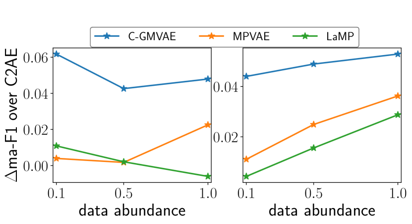
Figure 2: Relative improvements of C-GMVAE, MPVAE and LaMP on ma-F1 compared to C2AE. Left and right plots correspond to mirflickr and nus-vec datasets respectively. Every method (including C2AE) is trained on the same amount of data (10%, 50% or 100%) for comparison.

Full supervision

In the full supervision scenario, which is commonly adopted by the methods we compare against, we evaluate five metrics: example-F1 (ex-F1), micro-F1 (mi-F1), macro-F1 (ma-F1), Hamming accuracy (HA) and precision@1. The ex-F1 score is the averaged F1-score over all the samples. The mi-F1 score measures the aggregated contributions of all classes. The ma-F1 treats each class equally and takes the class-wise average. HA counts the correctly predicted labels regardless of samples or classes. The full definitions of these metrics can be found in the appendix.

Tab. 1, 2 and 3 present the performance of all the methods w.r.t. the metrics. We abbreviate nuswide-vector to nus-vec, and bookmarks to bkms. C-GMVAE outperforms the existing state-of-the-art methods on all the datasets. The best numbers are marked in bold. All the numbers for C-GMVAE are averaged over 3 seeds for stability and the standard deviations are included in the table. On ex-F1, C-GMVAE improves over ASL by 5.3%, RBCC by 7.7%, MPVAE by 2.5%, and LaMP by 8.8% on average across all the datasets. Similarly, on mi-F1, C-GMVAE improves over ASL by 4.4%, RBCC by 6.7%, MPVAE by 2.4% and LaMP 6.1% on average. On ma-F1, the improvements are as large as 6.1%, 9.4%, 4.1% and 11%, respectively. C-GMVAE outperforms other methods consistently.

Ablation study

To demonstrate the strength of C-GMVAE, we compare it with a unimodal Gaussian latent model, a Gaussian mixture only latent model (without contrastive module), and a contrastive learning only model (without the KL divergence term) in Tab. 5. Our C-GMVAE (GM+contrastive) consistently outperforms other models by a large margin. For instance, on ma-F1, C-GMVAE improves over the unimodal Gaussian model by 7%. In Tab. 7, we show that the contrastive module outperforms both the GNN and covariance matrix modules.

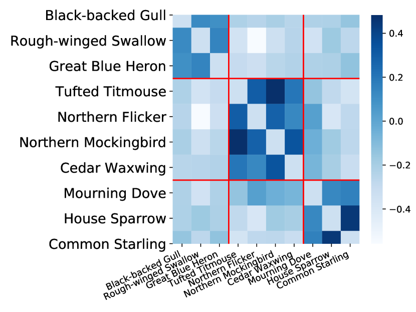
Figure 3: Label-label inner-products from C-GMVAE. One can compare it with Fig. 4 from MPVAE in the appendix. C-GMVAE demonstrates sharper and more meaningful inner-products.

Training on fewer data

Contrastive learning learns contrastive views and thus requires less information compared to generative learning, which demands a more complete representation for reconstruction. Contrastive learning has the potential to discover the intrinsic structure present in the data, and therefore is widely used in self-supervised learning because it generalizes well. We observe this with C-GMVAE as well. To demonstrate this, we shrink the size of training data by 50% or 90% and train methods on them. Surprisingly, we find C-GMVAE can often match the performance of other methods with only 50% of the training data. Tab. 6 compares MPVAE trained on all data and C-GMVAE trained on 50% of the data. Their performance is approximately the same. We further compare several major state-of-the-art methods including ours, all trained on the same randomly selected 10%, 50% and 100% of the data, and show their performance over C2AE. Fig. 2 shows the improvements over C2AE on ma-F1. Ours clearly outperforms the others with fewer data. More plots for other datasets and metrics are in the appendix.

Interpretability

Our work is also motivated by ecological applications (Gomes et al., 2019), where it is important to understand species interactions. Fig. 3 shows a map of inner-product weights of label embeddings on the eBird dataset. The bird species on the x-axis and the y-axis are the same. The first 3 bird species are water birds. The following 4 bird species are forest birds. The last 3 bird species are residential birds. Darker colors indicate more similar birds. We subtract the diagonal to exclude the self correlation. The heatmap matrix clearly forms three blocks on the diagonal. The first block contains Black-backed Gull, Rough-winged Swallow and Great Blue Heron. These three birds are water birds living near sea or lake. The second block has Tufted Titmouse, Northern Flicker, Northern Mockingbird, and Cedar Waxwing. These birds typically live in the forest with a lot of trees. The remaining birds are commonly seen residential birds, Mourning Dove, House Sparrow and Common Starling. They live inside or near human residences. Since human activities are wide-spread, the distribution of these birds is therefore quite broad. For example, the Mourning Dove is also correlated with forest birds in Fig. 3. But one can observe that for each group of birds, their intra-group correlations are always stronger than inter-group correlations. Therefore, the learnt embeddings do encompass semantic meanings. The derived correlations could also help the study of wildlife protection (Johnston et al., 2019).

5 Conclusion

In this work, we propose the contrastive learning boosted Gaussian mixture variational autoencoder (C-GMVAE), a novel method for multi-label prediction tasks. C-GMVAE combines the learning of Gaussian mixture latent spaces and the contrastive learning of feature and label embeddings. Not only does C-GMVAE achieve the state-of-the-art performance, it also provides insights into semi-supervised learning and model interpretability. Interesting future directions include the exploration of various contrastive learning mechanisms, model architecture improvements, and other latent space structures.

Appendix A Contrastive Learning Module

A.1 Connection with Triplet Loss

Triplet loss (Wang et al., 2014) is one of the popular ranking losses used in multi-label learning (Seymour & Zhang, 2018).

Given an anchor embedding $v_{x}^{f}$, a positive embedding $v_{+}$ and a negative embedding $v_{-}$, they form a triplet $(v_{x}^{f},v_{+},v_{-})$. A triplet loss is defined as

$$\mathcal{L}_{trip}(v_{x}^{f},v_{+},v_{-})$$ (9)

$$= max\{0,g+dist(v_{x}^{f},v_{+})-dist(v_{x}^{f},v_{-})\}$$

where $g$ is a gap parameter measuring the distance between $(v_{x}^{f},v_{+})$ and $(v_{x}^{f},v_{-})$, and $dist(\cdot,\cdot)$ is a distance function. This hinge loss $\mathcal{L}_{trip}$ encourages fewer violations to “positive$>$negative” ranking order. Let $\tau=1/2$. With the same triplet, we can write down a contrastive loss

$$\mathcal{L}_{CL}(v_{x}^{f},v_{+},v_{-})$$ (10)

$$= -\log\frac{\exp(2\cdot v^{f}_{x}\cdot v_{+})}{\sum_{t\in\{+,-\}}\exp(2\cdot v^{f}_{x}\cdot v_{t})}$$

$$= \log(1+\frac{\exp(2\cdot v^{f}_{x}\cdot v_{-})}{\exp(2\cdot v^{f}_{x}\cdot v_{+})})$$

$$\approx 1+(2\cdot v^{f}_{x}\cdot v_{-}-2\cdot v^{f}_{x}\cdot v_{+})$$

$$= 1+(-v_{x}^{f}\cdot v_{x}^{f}+2v^{f}_{x}\cdot v_{-}-v_{-}\cdot v_{-}$$

$$+v_{x}^{f}\cdot v_{x}^{f}-2\cdot v^{f}_{x}\cdot v_{+}+v_{+}\cdot v_{+})$$

$$= ||v_{x}^{f}-v_{+}||^{2}+||v_{x}^{f}-v_{-}||^{2}+1$$

Note that in the second to the last equation, $v_{+}$ and $v_{-}$ have the same norm due to the normalization in our contrastive learning module.

By setting $dist(\cdot,\cdot)$ to commonly used $\ell_{2}$ distance and $g=1$, Eq. 10 is a fair approximation of Eq. 9. Therefore, triplet loss can be viewed as a special case of contrastive loss. In contrastive loss, embeddings are normalized and more positives/negatives are available. As shown in (Chen et al., 2020), contrastive loss generally outperforms triplet loss.

A.2 Gradients of Contrastive Loss

Recall our contrastive loss:

$$\mathcal{L}_{CL}=\sum_{(x,y)\in\mathcal{B}}\frac{1}{|P(y)|}\sum_{p\in P(y)}-\log\frac{\exp(v^{f}_{x}\cdot v_{p}^{l}/\tau)}{\sum_{t\in A}\exp(v^{f}_{x}\cdot v_{t}^{l}/\tau)}$$ (11)

For the illustration purpose, we only consider one sample $(x,y)$ instead of one batch:

$$\mathcal{L}_{CL}=\frac{1}{|P(y)|}\sum_{p\in P(y)}-\log\frac{\exp(v^{f}_{x}\cdot v_{p}^{l}/\tau)}{\sum_{t\in A}\exp(v^{f}_{x}\cdot v_{t}^{l}/\tau)}$$ (12)

Define $N(y)\equiv A\setminus P(y)$. We now derive the gradients w.r.t. $v_{x}^{f}$.

$$\frac{\partial\mathcal{L}_{CL}}{\partial v_{x}^{f}}= \frac{1}{\tau|P(y)|}\sum_{p\in P(y)}(\frac{\sum_{t\in A}v_{t}^{l}\exp(v^{f}_{x}\cdot v_{t}^{l}/\tau)}{\sum_{t\in A}\exp(v^{f}_{x}\cdot v_{t}^{l}/\tau)}-v_{p}^{l})$$ (13)

$$= \frac{1}{\tau|P(y)|}\sum_{p\in P(y)}(\frac{\sum_{t\in P(y)}v_{t}^{l}\exp(v^{f}_{x}\cdot v_{t}^{l}/\tau)}{\sum_{t\in A}\exp(v^{f}_{x}\cdot v_{t}^{l}/\tau)}+$$

$$\frac{\sum_{t\in N(y)}v_{t}^{l}\exp(v^{f}_{x}\cdot v_{t}^{l}/\tau)}{\sum_{t\in A}\exp(v^{f}_{x}\cdot v_{t}^{l}/\tau)}-v_{p}^{l})$$

$$= \frac{1}{\tau}\frac{\sum_{t\in P(y)}v_{t}^{l}\exp(v^{f}_{x}\cdot v_{t}^{l}/\tau)}{\sum_{t\in A}\exp(v^{f}_{x}\cdot v_{t}^{l}/\tau)}+$$

$$\frac{1}{\tau}\frac{\sum_{t\in N(y)}v_{t}^{l}\exp(v^{f}_{x}\cdot v_{t}^{l}/\tau)}{\sum_{t\in A}\exp(v^{f}_{x}\cdot v_{t}^{l}/\tau)}-$$

$$\frac{1}{\tau|P(y)|}\sum_{p\in P(y)}v_{p}^{l}$$

$$= \frac{1}{\tau}[\sum_{t\in P(y)}v_{t}^{l}(\frac{\exp(v^{f}_{x}\cdot v_{t}^{l}/\tau)}{\sum_{a\in A}\exp(v^{f}_{x}\cdot v_{a}^{l}/\tau)}-\frac{1}{|P(y)|})+$$

$$\sum_{t\in N(y)}v_{t}^{l}\frac{\exp(v^{f}_{x}\cdot v_{t}^{l}/\tau)}{\sum_{a\in A}\exp(v^{f}_{x}\cdot v_{a}^{l}/\tau)}]$$

Further, we have the unnormalized feature embedding $w_{x}^{f}$, $v_{x}^{f}=\frac{w_{x}^{f}}{||w_{x}^{f}||}$.

$$\frac{\partial v_{x}^{f}}{\partial w_{x}^{f}}= \frac{1}{||w_{x}^{f}||}(I-\frac{w_{x}^{f}{w_{x}^{f}}^{T}}{||w_{x}^{f}||^{2}})=\frac{1}{||w_{x}^{f}||}(I-v_{x}^{f}{v_{x}^{f}}^{T})$$ (14)

where $I$ is an $E\times E$ identity matrix. The gradient of $\mathcal{L}_{CL}$ w.r.t. $w_{x}^{f}$ can be derived with chain rule,

$$\frac{\partial\mathcal{L}_{CL}}{\partial w_{x}^{f}}=\frac{\partial v_{x}^{f}}{\partial w_{x}^{f}}\frac{\partial\mathcal{L}_{CL}}{\partial v_{x}^{f}}$$ (15)

$$= \frac{1}{||w_{x}^{f}||}(I-v_{x}^{f}{v_{x}^{f}}^{T})\frac{1}{\tau}[\sum_{t\in P(y)}v_{t}^{l}(\frac{\exp(v^{f}_{x}\cdot v_{t}^{l}/\tau)}{\sum_{a\in A}\exp(v^{f}_{x}\cdot v_{a}^{l}/\tau)}$$

$$-\frac{1}{|P(y)|})+\sum_{t\in N(y)}v_{t}^{l}\frac{\exp(v^{f}_{x}\cdot v_{t}^{l}/\tau)}{\sum_{a\in A}\exp(v^{f}_{x}\cdot v_{a}^{l}/\tau)}]$$

$$= \frac{1}{\tau||w_{x}^{f}||}[\sum_{t\in P(y)}(v_{t}^{l}-(v_{x}^{f}v_{t}^{l})v_{x}^{f})(\frac{\exp(v^{f}_{x}\cdot v_{t}^{l}/\tau)}{\sum_{a\in A}\exp(v^{f}_{x}\cdot v_{a}^{l}/\tau)}$$

$$-\frac{1}{|P(y)|})+$$

$$\sum_{t\in N(y)}(v_{t}^{l}-(v_{x}^{f}v_{t}^{l})v_{x}^{f})\frac{\exp(v^{f}_{x}\cdot v_{t}^{l}/\tau)}{\sum_{a\in A}\exp(v^{f}_{x}\cdot v_{a}^{l}/\tau)}]$$

We can then observe that if $v_{x}^{f}$ and $v_{t}^{l}$ are orthogonal ($v_{x}^{f}v_{t}^{l}\to 0$), $||v_{t}^{l}-(v_{x}^{f}v_{t}^{l})v_{x}^{f}||$ will be close to 1 and the gradients would be large. Otherwise, for weak positives or negatives ($|v_{x}^{f}v_{t}^{l}|\to 1$), the gradients would be small.

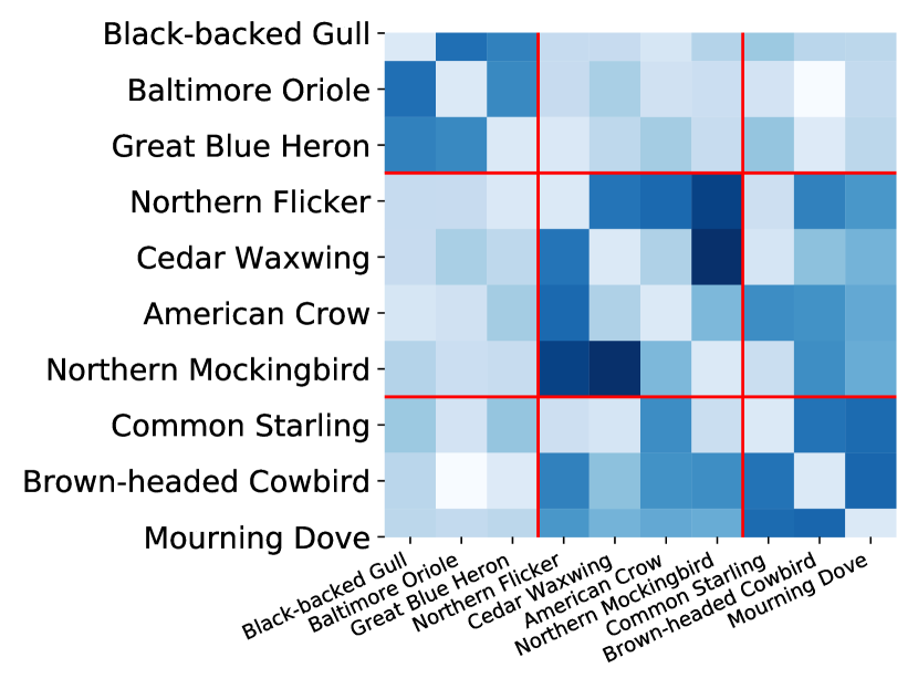
Figure 4: Label-label inner-products by MPVAE.

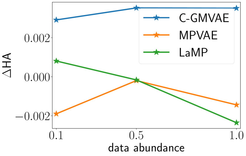
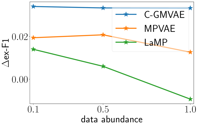
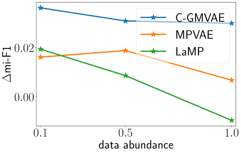
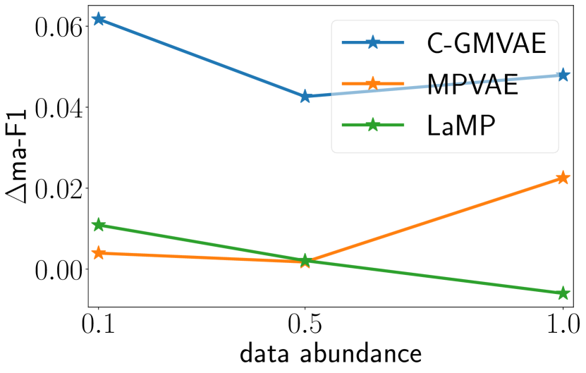
Figure 5: Relative performances w.r.t. HA, ex-F1, mi-F1 and ma-F1 on mirflickr dataset.

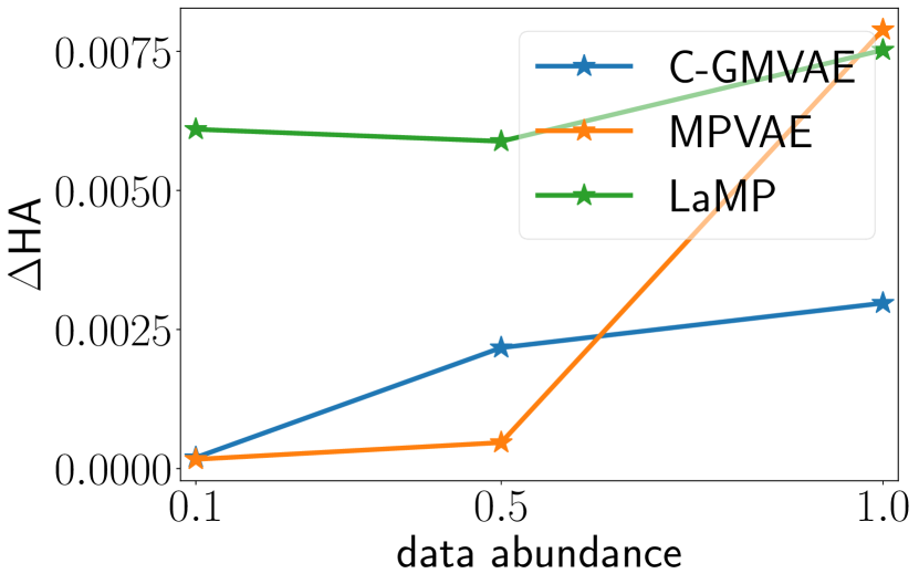
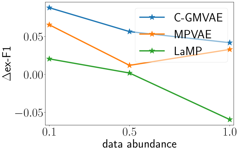
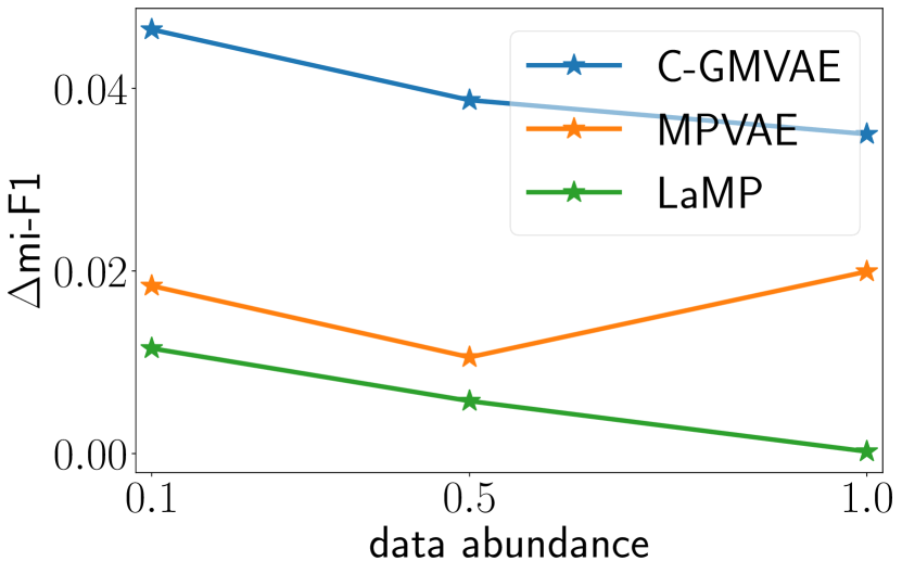
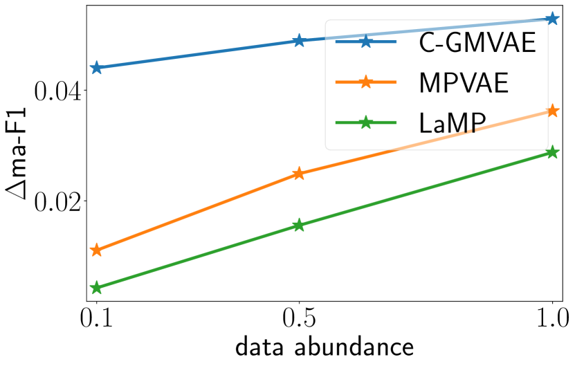
Figure 6: Relative performances w.r.t. HA, ex-F1, mi-F1 and ma-F1 on nus-vec dataset.

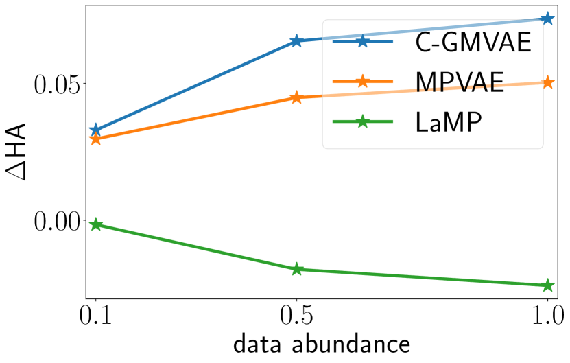
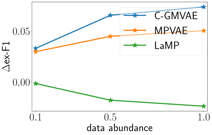
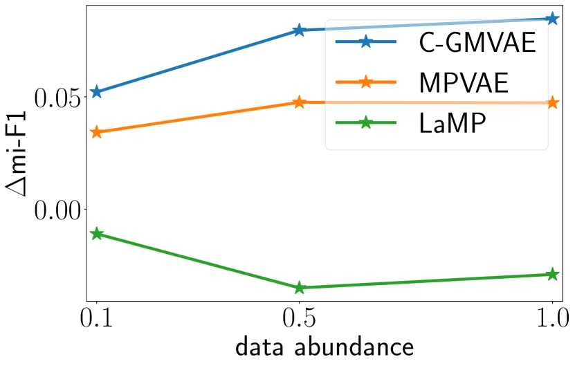
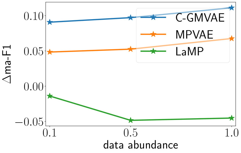
Figure 7: Relative performances w.r.t. HA, ex-F1, mi-F1 and ma-F1 on ebird dataset.

Appendix B Supplementary Experimental Results

B.1 Implementation Details

We use one Tesla V100 GPU on CentOS for every experiment. The batch size is set to 128. The latent dimensionality is 64. The feature encoder is an MLP with 3 hidden layers of sizes [256, 512, 256]. The label encoder has 2 hidden layers of sizes [512, 256]. The decoder contains 2 hidden layers of sizes [512, 512]. On reuters and bookmarks, we add one more hidden layer with 512 units to the decoder. The embedding size $E$ is 2048 (tuned within the range [512, 1024, 2048, 3072]). We set $\alpha=1$ (tuned within [0.1, 0.5, 1, 1.5, 2]), $\beta=0.5$ (tuned within [0.1, 0.5, 1, 1.5, 2.0]) for most runs. We tune learning rates from 0.0001 to 0.004 with interval 0.0002, dropout ratio from [0.3, 0.5, 0.7], and weight decay from [0, 0.01, 0.0001]. Grid search is adopted for tuning. Every batch in our experiments requires less than 16GB memory. The number of epochs is 100 by default.

model	eBird (s)		mirflickr (s)
	Train (per epoch)	Test (total)	Train (per epoch)	Test (total)
C2AE	27	29	18	24
LaMP	32	33	22	31
MPVAE	43	97	25	57
ASL	24	25	20	26
RBCC	3840	275	1320	337
C-GMVAE	22	24	14	16

Table 8: Comparison of different models’ time costs.

In Tab. 8, we show the per-epoch runtime for training, and the total time cost for testing. Our C-GMVAE is very competitive w.r.t. both training and testing time costs.

B.2 Training on Fewer Data

We provide relative performances of several major state-of-the-art methods including ours to C2AE, on HA, ex-F1, mi-F1, ma-F1 scores. All methods are trained on 10% or 50% of the data, including C2AE. The compared results have the same amount of data for training and thus the comparison is fair.

Fig. 5, Fig. 6, Fig. 7 show the relative performance of various state-of-the-art methods over C2AE, on mirflickr, nus-vec, eBird respectively.

References

- Annarumma & Montana (2017) Annarumma, M. and Montana, G. Deep metric learning for multi-labelled radiographs. arXiv preprint arXiv:1712.07682, 2017.
- Bai et al. (2020) Bai, J., Kong, S., and Gomes, C. Disentangled variational autoencoder based multi-label classification with covariance-aware multivariate probit model. IJCAI, 2020.
- Belanger & McCallum (2016) Belanger, D. and McCallum, A. Structured prediction energy networks. In International Conference on Machine Learning, 2016.
- Benites & Sapozhnikova (2015) Benites, F. and Sapozhnikova, E. Haram: a hierarchical aram neural network for large-scale text classification. In 2015 IEEE international conference on data mining workshop (ICDMW). IEEE, 2015.
- Bhatia et al. (2015) Bhatia, K., Jain, H., Kar, P., Varma, M., and Jain, P. Sparse local embeddings for extreme multi-label classification. Advances in neural information processing systems, 28:730–738, 2015.
- Bi & Kwok (2014) Bi, W. and Kwok, J. Multilabel classification with label correlations and missing labels. In Proceedings of the AAAI Conference on Artificial Intelligence, 2014.
- Boutell et al. (2004) Boutell, M. R., Luo, J., Shen, X., and Brown, C. M. Learning multi-label scene classification. Pattern recognition, 37(9):1757–1771, 2004.
- Chang et al. (2019) Chang, W.-C., Yu, H.-F., Zhong, K., Yang, Y., and Dhillon, I. X-bert: extreme multi-label text classification with using bidirectional encoder representations from transformers. arXiv preprint arXiv:1905.02331, 2019.
- Chen et al. (2019a) Chen, C., Wang, H., Liu, W., Zhao, X., Hu, T., and Chen, G. Two-stage label embedding via neural factorization machine for multi-label classification. In AAAI, 2019a.
- Chen et al. (2020) Chen, T., Kornblith, S., Norouzi, M., and Hinton, G. A simple framework for contrastive learning of visual representations. arXiv preprint arXiv:2002.05709, 2020.
- Chen et al. (2019b) Chen, Z.-M., Wei, X.-S., Wang, P., and Guo, Y. Multi-label image recognition with graph convolutional networks. In Proceedings of the IEEE/CVF Conference on Computer Vision and Pattern Recognition, pp. 5177–5186, 2019b.
- Chua et al. (2009) Chua, T.-S., Tang, J., Hong, R., Li, H., Luo, Z., and Zheng, Y. Nus-wide: a real-world web image database from national university of singapore. In Proceedings of the ACM international conference on image and video retrieval, pp. 1–9, 2009.
- Chung et al. (2015) Chung, J., Kastner, K., Dinh, L., Goel, K., Courville, A. C., and Bengio, Y. A recurrent latent variable model for sequential data. Advances in neural information processing systems, 28:2980–2988, 2015.
- Dao et al. (2021) Dao, S. D., Ethan, Z., Dinh, P., and Jianfei, C. Contrast learning visual attention for multi label classification. arXiv preprint arXiv:2107.11626, 2021.
- Debole & Sebastiani (2005) Debole, F. and Sebastiani, F. An analysis of the relative hardness of reuters-21578 subsets. Journal of the American Society for Information Science and technology, 56(6):584–596, 2005.
- Decubber et al. (2018) Decubber, S., Mortier, T., Dembczyński, K., and Waegeman, W. Deep f-measure maximization in multi-label classification: A comparative study. In Joint European Conference on Machine Learning and Knowledge Discovery in Databases, pp. 290–305. Springer, 2018.
- Dilokthanakul et al. (2016) Dilokthanakul, N., Mediano, P. A., Garnelo, M., Lee, M. C., Salimbeni, H., Arulkumaran, K., and Shanahan, M. Deep unsupervised clustering with gaussian mixture variational autoencoders. arXiv preprint arXiv:1611.02648, 2016.
- Doersch (2016) Doersch, C. Tutorial on variational autoencoders. arXiv preprint arXiv:1606.05908, 2016.
- Eslami et al. (2016) Eslami, S., Heess, N., Weber, T., Tassa, Y., Szepesvari, D., Kavukcuoglu, K., and Hinton, G. E. Attend, infer, repeat: Fast scene understanding with generative models. arXiv preprint arXiv:1603.08575, 2016.
- Fink et al. (2017) Fink, D., Auer, T., Obregon, F., Hochachka, W., Iliff, M., Sullivan, B., Wood, C., Davies, I., and Kelling, S. The ebird reference dataset version 2016 (erd2016), 2017.
- Gerych et al. (2021) Gerych, W., Hartvigsen, T., Buquicchio, L., Agu, E., and Rundensteiner, E. A. Recurrent bayesian classifier chains for exact multi-label classification. Advances in Neural Information Processing Systems, 34:15981–15992, 2021.
- Gomes et al. (2019) Gomes, C., Dietterich, T., et al. Computational sustainability: Computing for a better world and a sustainable future. Communications of the ACM, 62(9):56–65, 2019.
- Gutmann & Hyvärinen (2010) Gutmann, M. and Hyvärinen, A. Noise-contrastive estimation: A new estimation principle for unnormalized statistical models. In AISTATS, 2010.
- Huiskes & Lew (2008) Huiskes, M. J. and Lew, M. S. The mir flickr retrieval evaluation. In Proceedings of the 1st ACM international conference on Multimedia information retrieval, pp. 39–43, 2008.
- Johnston et al. (2019) Johnston, A., Hochachka, W., Strimas-Mackey, M., Gutierrez, V. R., Robinson, O., Miller, E., Auer, T., Kelling, S., and Fink, D. Best practices for making reliable inferences from citizen science data: case study using ebird to estimate species distributions. BioRxiv, pp. 574392, 2019.
- Katakis et al. (2008) Katakis, I., Tsoumakas, G., and Vlahavas, I. Multilabel text classification for automated tag suggestion. ECML PKDD Discovery Challenge, pp. 75, 2008.
- Khosla et al. (2021) Khosla, P., Teterwak, P., Wang, C., Sarna, A., Tian, Y., Isola, P., Maschinot, A., Liu, C., and Krishnan, D. Supervised contrastive learning. arXiv preprint arXiv:2004.11362, 2021.
- Kingma & Ba (2014) Kingma, D. P. and Ba, J. Adam: A method for stochastic optimization. arXiv:1412.6980, 2014.
- Kingma & Welling (2013) Kingma, D. P. and Welling, M. Auto-encoding variational bayes. arXiv:1312.6114, 2013.
- Koyejo et al. (2015) Koyejo, O., Natarajan, N., Ravikumar, P., and Dhillon, I. S. Consistent multilabel classification. In NIPS, volume 29, pp. 3321–3329, 2015.
- Kuhn et al. (2016) Kuhn, M., Letunic, I., Jensen, L. J., and Bork, P. The sider database of drugs and side effects. Nucleic acids research, 44(D1):D1075–D1079, 2016.
- Lanchantin et al. (2019) Lanchantin, J., Sekhon, A., and Qi, Y. Neural message passing for multi-label classification. arXiv preprint arXiv:1904.08049, 2019.
- Małkiński & Mańdziuk (2020) Małkiński, M. and Mańdziuk, J. Multi-label contrastive learning for abstract visual reasoning. arXiv preprint arXiv:2012.01944, 2020.
- Mikolov et al. (2013) Mikolov, T., Chen, K., Corrado, G., and Dean, J. Efficient estimation of word representations in vector space. arXiv preprint arXiv:1301.3781, 2013.
- Nakai & Kanehisa (1992) Nakai, K. and Kanehisa, M. A knowledge base for predicting protein localization sites in eukaryotic cells. Genomics, 14(4):897–911, 1992.
- Oord et al. (2018) Oord, A. v. d., Li, Y., and Vinyals, O. Representation learning with contrastive predictive coding. arXiv preprint arXiv:1807.03748, 2018.
- Read et al. (2009) Read, J., Pfahringer, B., Holmes, G., and Frank, E. Classifier chains for multi-label classification. In Joint European Conference on Machine Learning and Knowledge Discovery in Databases. Springer, 2009.
- Ridnik et al. (2021) Ridnik, T., Ben-Baruch, E., Zamir, N., Noy, A., Friedman, I., Protter, M., and Zelnik-Manor, L. Asymmetric loss for multi-label classification. In Proceedings of the IEEE/CVF International Conference on Computer Vision, pp. 82–91, 2021.
- Schönfeld et al. (2019) Schönfeld, E., Ebrahimi, S., Sinha, S., Darrell, T., and Akata, Z. Generalized zero-and few-shot learning via aligned variational autoencoders. In CVPR. IEEE, 2019.
- Seymour & Zhang (2018) Seymour, Z. and Zhang, Z. Multi-label triplet embeddings for image annotation from user-generated tags. In Proceedings of the 2018 ACM on International Conference on Multimedia Retrieval, pp. 249–256, 2018.
- Shi et al. (2019) Shi, Y., Siddharth, N., Paige, B., and Torr, P. H. Variational mixture-of-experts autoencoders for multi-modal deep generative models. arXiv preprint arXiv:1911.03393, 2019.
- Shi et al. (2020) Shi, Y., Paige, B., Torr, P. H., and Siddharth, N. Relating by contrasting: A data-efficient framework for multimodal generative models. arXiv preprint arXiv:2007.01179, 2020.
- Shu (2016) Shu, R. Gaussian mixture vae: Lessons in variational inference, generative models, and deep nets. 2016.
- Song & Ermon (2020) Song, J. and Ermon, S. Multi-label contrastive predictive coding. Advances in Neural Information Processing Systems, 33, 2020.
- Sundar et al. (2020) Sundar, V. K., Ramakrishna, S., Rahiminasab, Z., Easwaran, A., and Dubey, A. Out-of-distribution detection in multi-label datasets using latent space of -vae. arXiv preprint arXiv:2003.08740, 2020.
- Tomczak & Welling (2018) Tomczak, J. and Welling, M. Vae with a vampprior. In International Conference on Artificial Intelligence and Statistics, pp. 1214–1223. PMLR, 2018.
- Tsoumakas et al. (2008) Tsoumakas, G., Katakis, I., and Vlahavas, I. Effective and efficient multilabel classification in domains with large number of labels. In Proc. ECML/PKDD 2008 Workshop on Mining Multidimensional Data (MMD’08), volume 21, pp. 53–59, 2008.
- Tu & Gimpel (2018) Tu, L. and Gimpel, K. Learning approximate inference networks for structured prediction. arXiv preprint arXiv:1803.03376, 2018.
- Wang et al. (2021) Wang, F., Liu, H., Guo, D., and Sun, F. Unsupervised representation learning by invariancepropagation. arXiv preprint arXiv:2010.11694, 2021.
- Wang et al. (2014) Wang, J., Song, Y., Leung, T., Rosenberg, C., Wang, J., Philbin, J., Chen, B., and Wu, Y. Learning fine-grained image similarity with deep ranking. In Proceedings of the IEEE Conference on Computer Vision and Pattern Recognition, pp. 1386–1393, 2014.
- Wang et al. (2016) Wang, J., Yang, Y., Mao, J., Huang, Z., Huang, C., and Xu, W. Cnn-rnn: A unified framework for multi-label image classification. In CVPR, 2016.
- Wang & Wang (2019) Wang, P. Z. and Wang, W. Y. Neural gaussian copula for variational autoencoder. arXiv preprint arXiv:1909.03569, 2019.
- Wu & Goodman (2018) Wu, M. and Goodman, N. Multimodal generative models for scalable weakly-supervised learning. In Advances in Neural Information Processing Systems, 2018.
- Yeh et al. (2017) Yeh, C.-K., Wu, W.-C., Ko, W.-J., and Wang, Y.-C. F. Learning deep latent space for multi-label classification. In AAAI, 2017.
- Yu et al. (2013) Yu, G., Rangwala, H., Domeniconi, C., Zhang, G., and Yu, Z. Protein function prediction using multilabel ensemble classification. IEEE/ACM Transactions on Computational Biology and Bioinformatics, 2013.
- Zhang & Zhou (2007) Zhang, M.-L. and Zhou, Z.-H. Ml-knn: A lazy learning approach to multi-label learning. Pattern recognition, 40(7):2038–2048, 2007.
- Zhang & Zhou (2013) Zhang, M.-L. and Zhou, Z.-H. A review on multi-label learning algorithms. IEEE transactions on knowledge and data engineering, 2013.
- Zhang et al. (2018) Zhang, M.-L., Li, Y.-K., Liu, X.-Y., and Geng, X. Binary relevance for multi-label learning: an overview. Frontiers of Computer Science, 12(2):191–202, 2018.