On the enumeration of integer tetrahedra

Abstract

We consider the problem of enumerating integer tetrahedra of fixed perimeter (sum of side-lengths) and/or diameter (maximum side-length), up to congruence. As we will see, this problem is considerably more difficult than the corresponding problem for triangles, which has long been solved. We expect there are no closed-form solutions to the tetrahedron enumeration problems, but we explore the extent to which they can be approached via classical methods, such as orbit enumeration. We also discuss algorithms for computing the numbers, and present several tables and figures that can be used to visualise the data. Several intriguing patterns seem to emerge, leading to a number of natural conjectures. The central conjecture is that the number of integer tetrahedra of perimeter $n$, up to congruence, is asymptotic to $n^{5}/C$ for some constant $C\approx 229000$.

Keywords: Enumeration, integer tetrahedra, perimeter, orbit enumeration.

MSC: 52B05, 05A17, 05E18, 05A10.

James East, Michael Hendriksen, Laurence Park¹

1 Introduction

Geometry and combinatorics have many natural meeting points. Arguably the most ancient known example is the application of right-angled integer triangles in Babylonian architecture and agriculture. The classification of all such right triangles is recorded in Book X of Euclid’s Elements. Enumeration of arbitrary integer triangles goes back at least to the 1979 paper of Jordan, Walch and Wisner [11], and we have the following elegant result of Honsberger [8], which has been proved in a variety of ways [8, 10, 6, 7, 4, 5]:

Theorem.

The number of integer triangles with perimeter $n$, up to congruence, is the nearest integer to $\frac{n^{2}}{48}$ if $n$ is even, or to $\frac{(n+3)^{2}}{48}$ if $n$ is odd.

Two of the most natural extensions of this triangle enumeration problem are to consider integer polygons (increasing the number of sides), or integer tetrahedra (moving up a dimension). The former was treated in [4], and the current article considers the latter. Our main guiding problem is the following. By an integer tetrahedron we mean a (non-degenerate) tetrahedron whose sides are all of integer length, as in Figure 1. The perimeter of a tetrahedron is the sum of its six side-lengths.

Problem 1.

Calculate the number $t_{n}$ of integer tetrahedra with perimeter $n$, up to congruence: i.e., combinations of rotations, translations and reflections.

One might hope that $t_{n}$ is given by a similar formula to the triangle sequence in Honsberger’s Theorem above. As we will see, however, this is very far from the truth.

Philip Benjamin has computed $t_{n}$ for $n\leq 30$, but as far as we know has not published his methods; see [1, Sequence A208454]. Sascha Kurz [12] has considered the related problem of enumeration by diameter, defined to be the maximum of the six side-lengths:

Problem 2.

Calculate the number ${}^{d}t$ of integer tetrahedra with diameter $d$, up to congruence.

Kurz has computed ${}^{d}t$ for $d\leq 1000$ in [12]; see also [1, Sequence A097125]. The article [12] gives a lot of detail about Kurz’s methods and algorithms. No formula is given or conjectured, though an exact expression is given for a related set of (orbits of) matrices; this leads to a conjectural asymptotic formula, as we discuss in Sections 4.1 and 4.5.

It is not hard to show that the number of integer triangles with diameter $d$, up to congruence, is equal to $\big{\lfloor}\frac{(d+1)^{2}}{4}\big{\rfloor}$; see [1, Sequence A002620].

There is also of course the following natural problem, combining perimeter and diameter:

Problem 3.

Calculate the number ${}^{d}t_{n}$ of integer tetrahedra with perimeter $n$ and diameter $d$, up to congruence.

Clearly a solution to Problem 3 would yield solutions to Problems 1 and 2, since

$$t_{n}=\sum_{d}{}^{d}t_{n}\qquad\text{and}\qquad{}^{d}t=\sum_{n}{}^{d}t_{n}.$$

The non-zero terms in these sums occur for $\lceil\frac{n}{6}\rceil\leq d\leq\lfloor\frac{n-3}{3}\rfloor$ and $3d+3\leq n\leq 6d$, as we will show in Lemma 3.2.

Apart from this introduction, and a brief conclusion, the paper contains three further sections. In Section 2 we set up some ideas that (in principle) allow the calculation of $t_{n}$, ${}^{d}t$ and ${}^{d}t_{n}$ via Burnside’s Lemma, and we make some partial progress by giving explicit formulas for some of the relevant parameters. In Section 3 we discuss algorithms for computing the numbers $t_{n}$, ${}^{d}t$ and ${}^{d}t_{n}$, and give several tables and graphs of computed values; more data can be found at [3]. In Section 4 we explore some intriguing patterns that seem to emerge from an examination of the data. A number of conjectures/open problems are stated. We hope that these provide inspiration for future studies.

Figure 1: Two integer tetrahedra. The one on the left is tri-rectangular. The one on the right is invariant under a $120^{\circ}$ rotation about a vertical axis.

2 Enumeration via Burnside’s Lemma

In this section we focus on the numbers $t_{n}$, though all we say can easily be adapted to work for the numbers ${}^{d}t$ or ${}^{d}t_{n}$ instead. In Remark 2.13 we indicate the modifications needed for these.

Let $\mathcal{G}$ be the set of all edge-labelled graphs whose underlying unlabelled graph is the complete graph on vertex set $\{1,2,3,4\}$, and whose labels all belong to $\mathbb{N}=\{1,2,3,\ldots\}$. For $G\in\mathcal{G}$, we denote the label of the edge $\{i,j\}$ by $G(i,j)=G(j,i)$. The symmetric group $\mathcal{S}_{4}$ has a natural action on $\mathcal{G}$, denoted $(\sigma,G)\mapsto\sigma\cdot G$, and induced by permuting the vertices. For $G\in\mathcal{G}$ and $\sigma\in\mathcal{S}_{4}$, and for distinct $i,j\in\{1,2,3,4\}$, we have

$$(\sigma\cdot G)(i,j)=G(\sigma^{-1}(i),\sigma^{-1}(j)).$$ (2.1)

For example, Figure 2 illustrates the action of the permutations $(2,3)$, $(1,2,3)$, $(1,2,4,3)$ and $(1,4)(2,3)$, written in standard cycle notation.

Figure 2: The graph $G\in\mathcal{G}$ (centre), as well as $\sigma\cdot G$ for various permutations $\sigma$ from $\mathcal{S}_{4}$.

An integer tetrahedron $T$ may be represented by a graph $G$ from $\mathcal{G}$ as follows. Choose an ordering $1,2,3,4$ on the corners of $T$, and let the label of the edge $\{i,j\}$ from $G$ be the corresponding side-length from $T$. Different orderings on the vertices typically lead to different graphs, so that $T$ may be represented by up to $24$ such graphs. In fact, these graphs representing $T$ are precisely those belonging to the orbit of $G$ under the action of $\mathcal{S}_{4}$ given in (2.1). For example, the tetrahedra from Figure 1 may be represented by the graphs in Figure 3; the orbits of these graphs have size $24$ and $4$, respectively. It is clear that two tetrahedra are congruent if and only if they are represented by the same set of graphs from $\mathcal{G}$.

Figure 3: Graphs from $\mathcal{G}$ representing the tetrahedra pictured in Figure 1.

Not every graph from $\mathcal{G}$ corresponds to a tetrahedron in the above manner. For example, we claim that this is the case for the two graphs pictured in Figure 4. This is clear for the left-hand graph, as there is no triangle with edges $(1,1,2)$. However, the right-hand graph cannot be ruled out so easily, as the triples $(7,7,7)$ and $(7,4,4)$ do indeed correspond to triangles. Rather, the problem here is that if one tries to fold the “net” shown in Figure 5 (left) into a tetrahedron, then the tips of the three $(7,4,4)$ triangles do not meet.

Figure 4: Graphs from $\mathcal{G}$ not corresponding to tetrahedra.

Figure 5: Attempting to construct a tetrahedron from the graph in Figure 4 (right).

For $n\in\mathbb{N}$, let $\mathcal{T}_{n}$ be the set of graphs from $\mathcal{G}$ corresponding to some tetrahedron of perimeter $n$. The number of integer tetrahedra of perimeter $n$, up to congruence, is then given by the number $t_{n}=|\mathcal{T}_{n}/\mathcal{S}_{4}|$ of orbits of $\mathcal{T}_{n}$ under the action of $\mathcal{S}_{4}$ given in (2.1). Burnside’s Lemma (cf. [2, p. 246]) then gives

$$t_{n}=|\mathcal{T}_{n}/\mathcal{S}_{4}|=\frac{1}{24}\sum_{\sigma\in\mathcal{S}_{4}}\operatorname{fix}(\sigma).$$ (2.2)

Here, for $\sigma\in\mathcal{S}_{4}$, $\operatorname{fix}(\sigma)$ is the cardinality of the set

$$\operatorname{Fix}(\sigma)=\{G\in\mathcal{T}_{n}:\sigma\cdot G=G\}.$$ (2.3)

To enumerate tetrahedra up to rotations and translations only, we would be looking at orbits under the restricted action of the alternating group $\mathcal{A}_{4}\subseteq\mathcal{S}_{4}$, since even and odd permutations correspond to rotations and reflections, respectively. The number $t_{n}^{\prime}$ of integer tetrahedra of perimeter $n$, up to this kind of restricted congruence, is given by

$$t_{n}^{\prime}=|\mathcal{T}_{n}/\mathcal{A}_{4}|=\frac{1}{12}\sum_{\sigma\in\mathcal{A}_{4}}\operatorname{fix}(\sigma).$$ (2.4)

Thus, to calculate the numbers $t_{n}$ and $t_{n}^{\prime}$, it is enough to identify the set $\mathcal{T}_{n}$, and calculate the parameters $\operatorname{fix}(\sigma)$ for each $\sigma\in\mathcal{S}_{4}$. For the former, we have the following:

Proposition 2.5.

The set $\mathcal{T}_{n}$ consists of all graphs $G$ from $\mathcal{G}$ whose edge-labels, as shown in Figure 2 (centre), satisfy:

2. $A+B+C+a+b+c=n$,

3. $A+B+C>2\max(A,B,C)$,

4. $A+b+c>2\max(A,b,c)$,

5. $a+B+c>2\max(a,B,c)$,

6. $a+b+C>2\max(a,b,C)$,

7. $(a^{2}-B^{2}-c^{2}+2x_{1}x_{2})^{2}<4Y_{1}Y_{2}$, where

   • $x_{1}=\tfrac{A^{2}+B^{2}-C^{2}}{2A}$,

   • $x_{2}=\tfrac{A^{2}+c^{2}-b^{2}}{2A}$.

   • $Y_{1}=B^{2}-x_{1}^{2}$,

   • $Y_{2}=c^{2}-x_{2}^{2}$.

Proof.

First note that three positive real numbers $x,y,z$ can be the sides of a triangle if and only if the sum of the smaller two is greater than the largest; this is equivalent to $x+y+z>2\max(x,y,z)$. Thus, consulting Figure 2, it is clear that $\mathcal{T}_{n}$ is a subset of

$$\mathcal{T}_{n}^{\prime}=\big{\{}G\in\mathcal{G}:\text{\ref{T1}--\ref{T5} hold}\big{\}}.$$

Now consider a graph $G$ from $\mathcal{T}_{n}^{\prime}$, with edges labelled as in Figure 2. Then $G$ corresponds to a tetrahedron if and only if the following procedure can be carried out:

• Begin with the quadrilateral shown in Figure 6 (left).

• Keeping the $(A,B,C)$-triangle fixed in place, fold along the $x$-axis by some angle $0<\theta<\pi$ until the free tips of the two triangles are $a$ units apart, as shown in Figure 6 (middle). (We have strict inequalities for $\theta$ to ensure that the tetrahedron is not degenerate.)

Figure 6 (right) displays the two original triangles, as well as the result of folding by the angle $\theta=\pi$, and defines three points, $P,Q,R\in\mathbb{R}^{2}$. Let the coordinates of these points be $P=(x_{1},y_{1})$, $Q=(x_{2},y_{2})$ and $R=(x_{2},-y_{2})$. Also, put $Y_{1}=y_{1}^{2}$ and $Y_{2}=y_{2}^{2}$. It is easy to check that $x_{1},x_{2},Y_{1},Y_{2}$ are as given in (T6): e.g., consider $P$ as the intersection of the circles $x^{2}+y^{2}=B^{2}$ and $(x-A)^{2}+y^{2}=C^{2}$.

We claim that the above folding procedure can be carried out if and only if ${|PQ|<a<|PR|}$. Indeed, if we denote by $R_{\theta}\in\mathbb{R}^{3}$ the tip of the moving triangle after folding by the angle $0\leq\theta\leq\pi$, then $R_{\theta}=(x_{2},-y_{2}\cos\theta,y_{2}\sin\theta)$. It follows that $|PR_{\theta}|^{2}=(x_{1}-x_{2})^{2}+y_{1}^{2}+y_{2}^{2}+2y_{1}y_{2}\cos\theta$ is a smooth, decreasing function of $0\leq\theta\leq\pi$.

With the claim established, it remains to observe that the inequality $|PQ|<a<|PR|$ is equivalent to that in (T6), as

$$|PQ|<a<|PR| \ \Leftrightarrow\ |PQ|^{2}<a^{2}<|PR|^{2}$$

$$\ \Leftrightarrow\ (x_{1}-x_{2})^{2}+(y_{1}-y_{2})^{2}<a^{2}<(x_{1}-x_{2})^{2}+(y_{1}+y_{2})^{2}$$

$$\ \Leftrightarrow\ y_{1}^{2}+y_{2}^{2}-2y_{1}y_{2}<a^{2}-(x_{1}-x_{2})^{2}<y_{1}^{2}+y_{2}^{2}+2y_{1}y_{2}$$

$$\ \Leftrightarrow\ -2y_{1}y_{2}<a^{2}-(x_{1}-x_{2})^{2}-y_{1}^{2}-y_{2}^{2}<2y_{1}y_{2}$$

$$\ \Leftrightarrow\ (a^{2}-(x_{1}-x_{2})^{2}-y_{1}^{2}-y_{2}^{2})^{2}<4y_{1}^{2}y_{2}^{2}$$

$$\ \Leftrightarrow\ (a^{2}-B^{2}-c^{2}+2x_{1}x_{2})^{2}<4y_{1}^{2}y_{2}^{2}.\qed$$

Figure 6: Creating an integer tetrahedron; see the proof of Proposition 2.5 for further details.

Remark 2.6.

Items (T4) and (T5) from Proposition 2.5 are actually unnecessary. Indeed, given (T1)–(T3), and in the notation of the above proof (cf. Figure 6), (T6) is equivalent to the inequality $|PQ|<a<|PR|$. This ensures that the triples $(a,B,c)$ and $(a,b,C)$ correspond to triangles, which implies (T4) and (T5).

Alternative formulations of (T6) also exist. On [12, p. 3], Kurz attributes to Menger [13] the equivalent inequality involving a determinant:

$$\left|\begin{matrix}0&A^{2}&C^{2}&b^{2}&1\\ A^{2}&0&B^{2}&c^{2}&1\\ C^{2}&B^{2}&0&a^{2}&1\\ b^{2}&c^{2}&a^{2}&0&1\\ 1&1&1&1&0\end{matrix}\right|>0.$$

See also [14] for an elementary proof of this inequality, and a discussion of its history. Although the inequalities in Proposition 2.5 are less elegant (and symmetrical) than the above determinant inequality, they seem to be quicker to check computationally.

Now that we have characterised the set $\mathcal{T}_{n}$, it remains to calculate the values of $\operatorname{fix}(\sigma)$ for each ${\sigma\in\mathcal{S}_{4}}$. By symmetry we only have to do this for $\sigma$ being one of the following:

2. $\operatorname{id}_{4}$,

3. $(1,2,3)$,

4. $(1,4)(2,3)$,

5. $(2,3)$,

6. $(1,2,4,3)$.

In these cases, the number of elements of $\mathcal{S}_{4}$ with the same values of $\operatorname{fix}(\sigma)$ are, respectively, (i) 1, (ii) 8, (iii) 3, (iv) 6, (v) 6. Moreover, $\operatorname{Fix}(\sigma)$ may be characterised as the graphs $G$ from $\mathcal{T}_{n}$ whose labels (as in Figure 2) satisfy the following constraints, respectively:

2. NA,

3. $A=B=C$ and $a=b=c$,

4. $B=b$ and $C=c$,

5. $B=C$ and $b=c$,

6. $A=a$ and $B=C=b=c$.

In case (i) we have $\operatorname{fix}(\operatorname{id}_{4})=|\mathcal{T}_{n}|$. The next two results give exact formulas for $\operatorname{fix}(\sigma)$ when $\sigma$ has type (ii) or (v). We do not currently have formulas for types (i), (iii) or (iv); nor do we know if “neat” such formulas exist.

Lemma 2.7.

If $\sigma=(1,2,3)$, then

$$\operatorname{fix}(\sigma)=\begin{cases}0&\text{if $n\not\equiv 0\ (\operatorname{mod}3)$}\\ \big{\lfloor}\frac{n}{3+\sqrt{3}}\big{\rfloor}&\text{if $n\equiv 0\ (\operatorname{mod}3)$.}\end{cases}$$

Proof.

As noted above, $\operatorname{Fix}(\sigma)$ consists of the graphs from $\mathcal{T}_{n}$ whose edge-labels (as in Figure 2) satisfy $A=B=C$ and $a=b=c$. Such a graph corresponds to a tetrahedron of the form shown in Figure 7 (left). If such a tetrahedron exists, then from $n=3A+3a$ we must have $n\equiv 0\ (\operatorname{mod}3)$, and $a=\frac{n}{3}-A$. Then we note that (T2) is trivial, while (T3) is equivalent to the assertion that there is an $(A,a,a)$-triangle; the latter is equivalent to $A<2a$, and hence by integrality to $A+1\leq 2a=\frac{2n}{3}-2A$. Keeping in mind that $A$ is an integer, the latter gives

$$A \leq\left\lfloor\frac{2n-3}{9}\right\rfloor.$$ (2.8)

For (T6), we have $$x_{1}=x_{2}=\frac{A}{2} Y_{1}=\frac{3A^{2}}{4} Y_{2}=a^{2}-\frac{A^{2}}{4} {\frac{A^{4}}{4}<3A^{2}(a^{2}-\frac{A^{2}}{4})} A,a>0 A<\sqrt{3}a=\sqrt{3}(\frac{n}{3}-A) A<\frac{n}{3+\sqrt{3}} A \frac{n}{3+\sqrt{3}}$$, and , and the inequality in (T6) becomes . Rearranging, and remembering that , this gives , and so . Since is an integer, and since is irrational, it follows that

$$A \leq\left\lfloor\frac{n}{3+\sqrt{3}}\right\rfloor.$$ (2.9)

One may show that $\frac{2n-3}{9}\geq\frac{n}{3+\sqrt{3}}\ \Leftrightarrow\ n\geq 31$, and also that $\left\lfloor\frac{2n-3}{9}\right\rfloor=\big{\lfloor}\frac{n}{3+\sqrt{3}}\big{\rfloor}$ if $n\leq 30$ is a multiple of $3$. The result then follows from (2.8) and (2.9). ∎

Lemma 2.10.

If $\sigma=(1,2,4,3)$, then

$$\operatorname{fix}(\sigma)=\begin{cases}0&\text{if $n\not\equiv 0\ (\operatorname{mod}2)$}\\ \big{\lfloor}\frac{n}{4+4\sqrt{2}}\big{\rfloor}&\text{if $n\equiv 0\ (\operatorname{mod}4)$}\\ \big{\lfloor}\frac{n+2+2\sqrt{2}}{4+4\sqrt{2}}\big{\rfloor}&\text{if $n\equiv 2\ (\operatorname{mod}4)$.}\end{cases}$$

Proof.

This time $\operatorname{Fix}(\sigma)$ consists of the graphs from $\mathcal{T}_{n}$ whose edge-labels (as in Figure 2) satisfy $A=a$ and $B=C=b=c$. Such a graph corresponds to a tetrahedron of the form shown in Figure 7 (right). If such a tetrahedron exists, then from $n=2A+4B$ we must have $n\equiv 0\ (\operatorname{mod}2)$, $A\equiv\frac{n}{2}\ (\operatorname{mod}2)$ and $B=\frac{n-2A}{4}$. Then we note that (T2) and (T3) are both equivalent to $A<2B$, and hence to $A+1\leq 2B=\frac{n}{2}-A$. The latter gives

$$A \leq\left\lfloor\frac{n-2}{4}\right\rfloor.$$ (2.11)

Rather than (T6), it is more convenient to work with the equivalent $$|PQ|^{2}<a^{2}<|PR|^{2} P=Q A=a A^{2}<4B^{2}-A^{2} A<\sqrt{2}B=\frac{n-2A}{2\sqrt{2}}$$ from the proof of Proposition 2.5; cf. Figure 6. Since (and remembering that , etc.), this is equivalent to , which gives , and ultimately

$$A \leq\left\lfloor\frac{n}{2+2\sqrt{2}}\right\rfloor.$$ (2.12)

This time, $\frac{n-2}{4}\geq\frac{n}{2+2\sqrt{2}}\ \Leftrightarrow\ n\geq 12$, and also $\left\lfloor\frac{n-2}{4}\right\rfloor=\big{\lfloor}\frac{n}{2+2\sqrt{2}}\big{\rfloor}$ if $n\leq 10$ is even. Thus, if we write $K=\big{\lfloor}\frac{n}{2+2\sqrt{2}}\big{\rfloor}$, then it follows from (2.11) and (2.12) that $\operatorname{fix}(\sigma)$ is equal to the cardinality of the set

$$X=\big{\{}A\in\mathbb{N}:A\leq K,\ A\equiv\tfrac{n}{2}\ (\operatorname{mod}2)\big{\}}.$$

Now,

$$|X|=\begin{cases}\lfloor\frac{K}{2}\rfloor&\text{if $\tfrac{n}{2}\equiv 0\ (\operatorname{mod}2)$: i.e., if $n\equiv 0\ (\operatorname{mod}4)$}\\ \lfloor\frac{K+1}{2}\rfloor&\text{if $\tfrac{n}{2}\equiv 1\ (\operatorname{mod}2)$: i.e., if $n\equiv 2\ (\operatorname{mod}4)$.}\end{cases}$$

The result then follows from the definition of $K$, and the fact that $\big{\lfloor}\frac{\lfloor x\rfloor}{2}\big{\rfloor}=\left\lfloor\frac{x}{2}\right\rfloor$ for real $x$. ∎

Figure 7: Tetrahedra from the proofs of Lemmas 2.7 and 2.10.

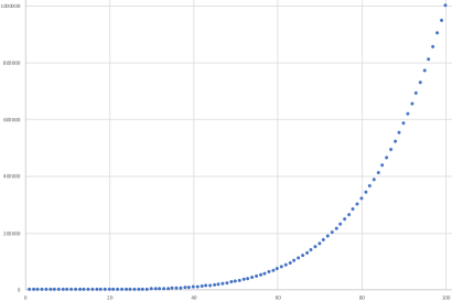
Figure 17: Calculated values of $\operatorname{fix}(\sigma)$, for $\sigma$ of type (i), $1\leq n\leq 100$.

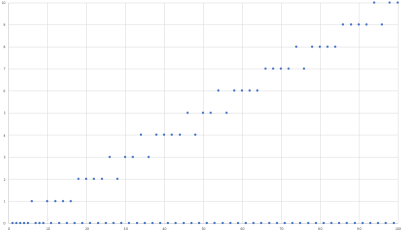
Figure 18: Left and right: calculated values of $\operatorname{fix}(\sigma)$, for $\sigma$ of type (ii) and (v), $1\leq n\leq 100$; cf. Lemmas 2.7 and 2.10.

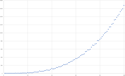
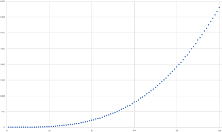
Figure 19: Left and right: calculated values of $\operatorname{fix}(\sigma)$, for $\sigma$ of type (iii) and (iv), $1\leq n\leq 100$.

As noted above, we are currently unable to calculate $\operatorname{fix}(\sigma)$ for $\sigma$ of types (i), (iii) and (iv). It is possible that types (iii) and (iv) could be treated by more elaborate versions of the arguments given in Lemmas 2.7 and 2.10. Calculated values of all $\operatorname{fix}(\sigma)$ parameters for $1\leq n\leq 100$ are given in Table 5; see also Figures 17–19. If one could calculate $\operatorname{fix}(\operatorname{id}_{4})=|\mathcal{T}_{n}|$, this would have important consequences for the asymptotics of $t_{n}$ itself; see Section 4.1.

Remark 2.13.

The arguments of this section can be modified to calculate the numbers ${}^{d}t$ or ${}^{d}t_{n}$. Consider the following condition on a graph $G$ from $\mathcal{G}$, as shown in Figure 2 (centre):

1. $\max\{A,B,C,a,b,c\}=d$.

Then the set ${}^{d}\mathcal{T}$ of graphs from $\mathcal{G}$ corresponding to integer tetrahedra of diameter $d$ are precisely those satisfying (T1)^′ and (T2)–(T6); cf. Proposition 2.5. The set ${}^{d}\mathcal{T}_{n}=\mathcal{T}_{n}\cap{}^{d}\mathcal{T}$ of graphs from $\mathcal{G}$ corresponding to integer tetrahedra of perimeter $n$ and diameter $d$ are precisely those satisfying (T1)^′ and (T1)–(T6). Then

$${}^{d}t=|{}^{d}\mathcal{T}/\mathcal{S}_{4}|\qquad\text{and}\qquad{}^{d}t_{n}=|{}^{d}\mathcal{T}_{n}/\mathcal{S}_{4}|$$

are given by counting orbits of the action of $\mathcal{S}_{4}$ given in (2.1). We also have the numbers ${}^{d}t^{\prime}$ and ${}^{d}t_{n}^{\prime}$, counting tetrahedra (of relevant parameters) up to rotations only, and these are given in terms of the restricted action of $\mathcal{A}_{4}$.

3 Computation and data

In the previous section we gave a method for (in principle) computing the numbers $t_{n}$, ${}^{d}t$ and ${}^{d}t_{n}$. Given that we are currently unable to give explicit formulas for the $\operatorname{fix}(\sigma)$ parameters in certain cases, and hence for the $t_{n}$, ${}^{d}t$ and ${}^{d}t_{n}$ sequences themselves, we now turn to some computations to make further progress. In this section we discuss algorithms/code, and give several tables and graphs of calculated values. In the next section we make some observations and conjectures based on the computational data.

3.1 Enumeration algorithms

To compute or enumerate all tetrahedra of a given perimeter $n$, we identify the graph $G$ from Figure 2 with the 6-tuple $\big{[}(A,a),(B,b),(C,c)\big{]}$. This is clearly a tuple over $\{1,\ldots,n\}$, though we will see in Lemma 3.2 that the entries of the tuple belong to a much smaller range; at this point, it is obvious at least that no entry could be bigger than $n-5$. The orbits of $G$ (as in Figure 2) under the action of $\mathcal{S}_{4}$ given in (2.1) correspond to the following tuples:

$$\big{[}(A,a),(B,b),(C,c)\big{]}, \big{[}(A,a),(b,B),(c,C)\big{]}, \big{[}(a,A),(B,b),(c,C)\big{]}, \big{[}(a,A),(b,B),(C,c)\big{]},$$

$$\big{[}(C,c),(A,a),(B,b)\big{]}, \big{[}(c,C),(A,a),(b,B)\big{]}, \big{[}(c,C),(a,A),(B,b)\big{]}, \big{[}(C,c),(a,A),(b,B)\big{]},$$

$$\big{[}(B,b),(C,c),(A,a)\big{]}, \big{[}(b,B),(c,C),(A,a)\big{]}, \big{[}(B,b),(c,C),(a,A)\big{]}, \big{[}(b,B),(C,c),(a,A)\big{]},$$

$$\big{[}(A,a),(C,c),(B,b)\big{]}, \big{[}(A,a),(c,C),(b,B)\big{]}, \big{[}(a,A),(c,C),(B,b)\big{]}, \big{[}(a,A),(C,c),(b,B)\big{]},$$

$$\big{[}(B,b),(A,a),(C,c)\big{]}, \big{[}(b,B),(A,a),(c,C)\big{]}, \big{[}(B,b),(a,A),(c,C)\big{]}, \big{[}(b,B),(a,A),(C,c)\big{]},$$

$$\big{[}(C,c),(B,b),(A,a)\big{]}, \big{[}(c,C),(b,B),(A,a)\big{]}, \big{[}(c,C),(B,b),(a,A)\big{]}, \big{[}(C,c),(b,B),(a,A)\big{]}.$$

Each of these can be alternatively obtained from $\big{[}(A,a),(B,b),(C,c)\big{]}$ by the action of a signed permutation $\tau$ of the set $\{1,2,3\}$. Roughly speaking, the non-signed part of $\tau$ tells us how to move the pairs $(A,a)$, $(B,b)$ and $(C,c)$, and the signed part tells us whether $(X,x)$ is listed in the final arrangement as $(X,x)$ or is flipped to $(x,X)$. Moreover, examining (LABEL:e:tuples), only those signed permutations with an even number of flips occur. This means that we are dealing with an action of the Coxeter group of type $D_{3}$, which is well-known to be isomorphic to the symmetric group $\mathcal{S}_{4}$ (type $A_{3}$). For more on Coxeter groups, see [9].

The most obvious algorithm for creating the set $\mathcal{T}_{n}$ would be to take all 6-tuples $\big{[}(A,a),(B,b),(C,c)\big{]}$ over $\{1,\ldots,n-5\}$, and keep those satisfying conditions (T1)–(T6) from Proposition 2.5. Once we have the set $\mathcal{T}_{n}$, we can quickly compute the tuples fixed under the action of permutations $\sigma$ from $\mathcal{S}_{4}$ of types (i)–(v), and thereby compute $t_{n}=\frac{1}{24}\sum_{\sigma}\operatorname{fix}(\sigma)$.

On the other hand, since we are ultimately concerned with counting orbits, we do not need to store all tuples from $\mathcal{T}_{n}$; we only need to store a single representative: e.g., the lex-greatest such tuple.

Some simple geometrical considerations allow us to reduce the search space, and also lead to other shortcuts.

Lemma 3.2.

If an integer tetrahedron has perimeter $n$ and diameter $d$, then

$$\Big{\lceil}\frac{n}{6}\Big{\rceil}\leq d\leq\Big{\lfloor}\frac{n-3}{3}\Big{\rfloor}\qquad\text{or equivalently}\qquad 3d+3\leq n\leq 6d.$$

Proof.

It suffices to prove the second system of inequalities, and we note that $n\leq 6d$ is clear.

Consider the graph $G$ pictured in Figure 2, and assume by symmetry that $d=A$. From the $(A,B,C)$- and $(A,b,c)$-triangles we obtain $B+C\geq A+1$ and $b+c\geq A+1$, and so

$$n=A+(B+C)+a+(b+c)\geq A+(A+1)+1+(A+1)=3d+3.\qed$$

Remark 3.3.

For fixed $d$, the maximum value of $n=6d$ occurs uniquely, of course, for the equilateral tetrahedron $\big{[}(d,d),(d,d),(d,d)\big{]}$. The minimum value of $n=3d+3$ corresponds to $\big{[}(1,d),(1,d),(1,d)\big{]}$, for example, a very “thin” tetrahedron of the form shown in Figure 7 (left). In general, other tetrahedra have $n=3d+3$: e.g., $\big{[}(1,d),(2,d-1),(2,d-1)\big{]}$ for $d\geq 3$.

Remark 3.4.

Although every edge of an integer teterahedron of perimeter $n$ is bounded above by $\lfloor\frac{n-3}{3}\rfloor$, it is not true that $\lceil\frac{n}{6}\rceil$ is a lower bound for all edges. Indeed, we have the very “thin” tetrahedra $\big{[}(1,d),(1,d),(1,d)\big{]}$ and $\big{[}(d,d),(d,d),(1,1)\big{]}$, as in Figure 7.

Similar considerations apply to the triangular faces:

Lemma 3.5.

If an integer tetrahedron has perimeter $n$ and maximum face-perimeter $M$, then

$$\Big{\lceil}\frac{n}{2}\Big{\rceil}\leq M\leq\Big{\lfloor}\frac{2n-3}{3}\Big{\rfloor}\qquad\text{or equivalently}\qquad\Big{\lceil}\frac{3M+3}{2}\Big{\rceil}\leq n\leq 2M.$$

Proof.

It suffices to show that $\frac{3M+3}{2}\leq n\leq 2M$. To do so, consider the graph $G$ pictured in Figure 2, assuming by symmetry that $M=A+B+C$. Adding the perimeters of all four faces gives twice the perimeter of the tetrahedron. The first consequence of this is that $2n\leq 4M$: i.e., $n\leq 2M$. The second consequence (also using $b+c\geq A+1$, etc., from the other triangular faces) is that

$$2n =(A+B+C)+(A+b+c)+(B+a+c)+(C+a+b)$$

$$\geq(A+B+C)+(A+A+1)+(B+B+1)+(C+C+1)=3(A+B+C)+3=3M+3,$$

which gives $n\geq\frac{3M+3}{3}$. ∎

With the above considerations in mind, a simple algorithm for calculating a set of representatives of ${}^{d}\mathcal{T}_{n}$ is as follows. Here we write $d=A$ to keep the notation as in Figure 2. Roughly speaking, we create tetrahedra as in Figure 6, with the diameter on the $x$-axis.

1. Define the set $S=\varnothing$.

2. Create the set of all triangles with maximum side $A({}=d)$ and with perimeter at most $\left\lfloor\tfrac{2n-3}{3}\right\rfloor$. (This is fairly routine, so the details are omitted.)

3. Then for each pair $(A,B,C)$ and $(A,b,c)$ of such triangles, we set $a={n-(A+B+C+b+c)}$.

4. If $a\leq A$ and if the tuple $T=\big{[}(A,a),(B,b),(C,c)\big{]}$ satisfies condition (T6) from Proposition 2.5, we add to the set $S$ the lex-greatest representative of $T$ from the list (LABEL:e:tuples).

The number ${}^{d}t_{n}={}^{A}t_{n}$ is then the size of the set $S$ created. Summing over all $d$ (or $n$) gives $t_{n}$ (or ${}^{d}t$), respectively. There are many easy ways to simplify the above. For example, the sixth entry of the tuple $\big{[}(A,a),(B,b),(C,c)\big{]}$ does not need to be stored, as it can be inferred from the others; neither do we need to store the first entry as this is always $d$ (this is why we chose to store the lex-greatest representative).

We carried out the above algorithm in a variety of languages. We were able to calculate $t_{n}$ up to $n=1100$ before running out of memory on standard laptops (even for single values of $d$). It was around this stage in our investigations that we discovered Kurz’s article [12]. We regret to say that the “integral” rather than “integer” in his title defeated our searching abilities. Additionally, since we were initially interested only in the $t_{n}$ sequence, we initially found only Sequence A208454 on the OEIS [1], but not A097125, which contains many terms in the ${}^{d}t$ sequence.

The most significant advantage of Kurz’s algorithm for enumeration by diameter is that it does not require the creation and storage of vast numbers of tuples. Rather, it moves through “tuple space” in such an orderly fashion that each canonical tuple is visited once, meaning that these only have to be counted rather than stored. Our current algorithms are modifications of Kurz’s, implemented in C, and with a number of optimisations, including parallelisation and use of the GNU Multiple Precision Arithmetic Library to store and manipulate large integers. All of our calculations of the numbers ${}^{d}t$ match those given by Kurz, though we have gone somewhat further; see Table 8.

3.2 Values

So far we have calculated $t_{n}$ for every $1\leq n\leq 3000$, and for several other values up to $n=20000$. Various tables and figures in this section summarise some of these calculations, but more complete lists are available at [3]. Some of the tables below also include values of ${}^{d}t$, ${}^{d}t_{n}$ and $t_{n}^{\prime}$ (tetrahedra up to rotations and translations only), and also $\operatorname{fix}(\sigma)$ for certain permutations $\sigma\in\mathcal{S}_{4}$. (More extensive tables containing values of ${}^{d}t$ are given by Kurz [12].) For convenience of reference, here is a summary of the content of the tables and figures given in this section (more are given in Section 4, and we note that some of the tables in the current section also include additional parameters defined in Section 4):

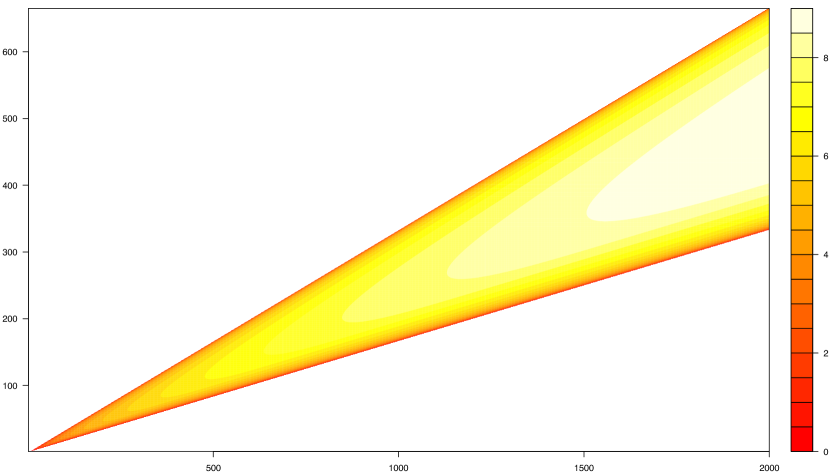
Figure 12: Heat map of the numbers $\log_{10}({}^{d}t_{n})$, with $1\leq n\leq 2000$ and $1\leq d\leq 666$ on the horizontal and vertical axes, respectively.

Location	Numbers	Range	Comments
Table 1	$t_{n}$	$1\leq n\leq 200$
Table 2	$t_{n}$	$1\leq n\leq 10000$	by hundreds
Table 3	${}^{d}t_{n}$	$1\leq n\leq 50$
Table 4	${}^{d}t_{n}$	$1\leq n\leq 200$
Table 5	$\operatorname{fix}(\sigma)$, $t_{n}$, $t_{n}^{\prime}$	$1\leq n\leq 100$
Table 7	$t_{n}$	$1\leq n\leq 20000$	by thousands
Table 8	${}^{d}t$	$1\leq d\leq 2000$	by hundreds
Figure 8	$t_{n}$	$1\leq n\leq 30$
Figure 9	$t_{n}$	$1\leq n\leq 200$
Figure 10	$t_{n}$	$1\leq n\leq 200$	log-log plot
Figure 11	$t_{n}$	$1\leq n\leq 10000$	by hundreds
Figure 12	${}^{d}t_{n}$	$1\leq n\leq 2000$	heat map
Figure 13	${}^{d}t_{n}$	$n=100$ and $200$
Figure 14	${}^{d}t_{n}$	$n=10000$	and discrete derivative
Figure 15	${}^{d}t_{n}$	$d=50$ and $100$
Figure 16	${}^{d}t_{n}$	$d=1000$	and discrete derivative
Figures 17–19	$\operatorname{fix}(\sigma)$	$1\leq n\leq 100$	$\sigma\in\mathcal{S}_{4}$

$n$	$t_{n}$
$1$	$0$
$2$	$0$
$3$	$0$
$4$	$0$
$5$	$0$
$6$	$1$
$7$	$0$
$8$	$0$
$9$	$1$
$10$	$1$
$11$	$1$
$12$	$3$
$13$	$2$
$14$	$3$
$15$	$6$
$16$	$6$
$17$	$7$
$18$	$12$
$19$	$11$
$20$	$18$
$21$	$21$
$22$	$25$
$23$	$31$
$24$	$38$
$25$	$46$
$26$	$56$
$27$	$66$
$28$	$76$
$29$	$90$
$30$	$117$
$31$	$123$
$32$	$151$
$33$	$175$
$34$	$196$
$35$	$234$
$36$	$264$
$37$	$297$
$38$	$346$
$39$	$391$
$40$	$448$

$n$	$t_{n}$
$41$	$492$
$42$	$568$
$43$	$630$
$44$	$702$
$45$	$797$
$46$	$884$
$47$	$977$
$48$	$1089$
$49$	$1217$
$50$	$1338$
$51$	$1469$
$52$	$1624$
$53$	$1771$
$54$	$1970$
$55$	$2146$
$56$	$2343$
$57$	$2579$
$58$	$2782$
$59$	$3042$
$60$	$3322$
$61$	$3586$
$62$	$3912$
$63$	$4221$
$64$	$4568$
$65$	$4953$
$66$	$5339$
$67$	$5731$
$68$	$6204$
$69$	$6657$
$70$	$7169$
$71$	$7683$
$72$	$8230$
$73$	$8857$
$74$	$9446$
$75$	$10095$
$76$	$10846$
$77$	$11513$
$78$	$12345$
$79$	$13125$
$80$	$13969$

$n$	$t_{n}$
$81$	$14903$
$82$	$15790$
$83$	$16811$
$84$	$17854$
$85$	$18940$
$86$	$20107$
$87$	$21261$
$88$	$22511$
$89$	$23831$
$90$	$25251$
$91$	$26631$
$92$	$28173$
$93$	$29744$
$94$	$31341$
$95$	$33116$
$96$	$34849$
$97$	$36696$
$98$	$38695$
$99$	$40619$
$100$	$42817$
$101$	$44951$
$102$	$47257$
$103$	$49641$
$104$	$52008$
$105$	$54685$
$106$	$57310$
$107$	$60046$
$108$	$62944$
$109$	$65896$
$110$	$69029$
$111$	$72152$
$112$	$75549$
$113$	$78976$
$114$	$82574$
$115$	$86199$
$116$	$90052$
$117$	$94053$
$118$	$98089$
$119$	$102371$
$120$	$106711$

$n$	$t_{n}$
$121$	$111246$
$122$	$116006$
$123$	$120768$
$124$	$125837$
$125$	$130985$
$126$	$136402$
$127$	$141853$
$128$	$147575$
$129$	$153500$
$130$	$159470$
$131$	$165757$
$132$	$172253$
$133$	$178772$
$134$	$185682$
$135$	$192674$
$136$	$200070$
$137$	$207440$
$138$	$215111$
$139$	$223151$
$140$	$231179$
$141$	$239687$
$142$	$248292$
$143$	$257130$
$144$	$266522$
$145$	$275691$
$146$	$285536$
$147$	$295385$
$148$	$305605$
$149$	$316146$
$150$	$326952$
$151$	$337891$
$152$	$349316$
$153$	$361051$
$154$	$372976$
$155$	$385325$
$156$	$398032$
$157$	$410750$
$158$	$424249$
$159$	$437744$
$160$	$451759$

$n$	$t_{n}$
$161$	$466128$
$162$	$480898$
$163$	$495924$
$164$	$511275$
$165$	$527179$
$166$	$543486$
$167$	$559950$
$168$	$576987$
$169$	$594453$
$170$	$612306$
$171$	$630619$
$172$	$649344$
$173$	$668273$
$174$	$688082$
$175$	$708017$
$176$	$728557$
$177$	$749759$
$178$	$770893$
$179$	$792983$
$180$	$815666$
$181$	$838151$
$182$	$862084$
$183$	$885874$
$184$	$910270$
$185$	$935691$
$186$	$960959$
$187$	$987344$
$188$	$1014149$
$189$	$1041441$
$190$	$1069393$
$191$	$1097727$
$192$	$1127002$
$193$	$1156747$
$194$	$1186965$
$195$	$1217963$
$196$	$1249657$
$197$	$1281804$
$198$	$1314840$
$199$	$1348514$
$200$	$1382630$

Table 1: Calculated values of $t_{n}$.

$n$	$t_{n}$
$100$	$42817$
$200$	$1382630$
$300$	$10542791$
$400$	$44512930$
$500$	$135995968$
$600$	$338647149$
$700$	$732301457$
$800$	$1428244253$
$900$	$2574424362$
$1000$	$4360687860$
$1100$	$7024066455$
$1200$	$10853927088$
$1300$	$16197354205$
$1400$	$23464200340$
$1500$	$33132516713$
$1600$	$45753651322$
$1700$	$61957547844$
$1800$	$82458026396$
$1900$	$108057877719$
$2000$	$139654346301$

$n$	$t_{n}$
$2100$	$178244109766$
$2200$	$224928623704$
$2300$	$280919515766$
$2400$	$347543441363$
$2500$	$426247856357$
$2600$	$518605683615$
$2700$	$626321040933$
$2800$	$751234199645$
$2900$	$895326815879$
$3000$	$1060727392377$
$3100$	$1249716260424$
$3200$	$1464730980692$
$3300$	$1708371608956$
$3400$	$1983405792552$
$3500$	$2292773954230$
$3600$	$2639594896693$
$3700$	$3027170849616$
$3800$	$3458992238494$
$3900$	$3938743901688$
$4000$	$4470309160343$

$n$	$t_{n}$
$4100$	$5057776483155$
$4200$	$5705443122022$
$4300$	$6417821623924$
$4400$	$7199644279518$
$4500$	$8055868989730$
$4600$	$8991684402358$
$4700$	$10012513881131$
$4800$	$11124023171269$
$4900$	$12332123259033$
$5000$	$13642977397892$
$5100$	$15063004902111$
$5200$	$16598887173873$
$5300$	$18257573582602$
$5400$	$20046284952842$
$5500$	$21972520100932$
$5600$	$24044061595649$
$5700$	$26268978527115$
$5800$	$28655635295636$
$5900$	$31212693377826$
$6000$	$33949118928429$

$n$	$t_{n}$
$6100$	$36874187631384$
$6200$	$39997488181501$
$6300$	$43328930438429$
$6400$	$46878747743940$
$6500$	$50657504819100$
$6600$	$54676100750626$
$6700$	$58945775513454$
$6800$	$63478115036529$
$6900$	$68285056161851$
$7000$	$73378891579018$
$7100$	$78772276600831$
$7200$	$84478231957643$
$7300$	$90510152207309$
$7400$	$96881807240927$
$7500$	$103607350139966$
$7600$	$110701321888040$
$7700$	$118178657158659$
$7800$	$126054687371188$
$7900$	$134345147515787$
$8000$	$143066182224551$

$n$	$t_{n}$
$8100$	$152234350689174$
$8200$	$161866628410449$
$8300$	$171980417994570$
$8400$	$182593551239230$
$8500$	$193724293506541$
$8600$	$205391352861569$
$8700$	$217613878464370$
$8800$	$230411473926234$
$8900$	$243804197732022$
$9000$	$257812568218126$
$9100$	$272457573348976$
$9200$	$287760666512263$
$9300$	$303743784383639$
$9400$	$320429342544289$
$9500$	$337840242823660$
$9600$	$355999882739690$
$9700$	$374932153990010$
$9800$	$394661455344190$
$9900$	$415212690326932$
$10000$	$436611276762080$

Table 2: Calculated values of $t_{n}$.

$n/d$	$1$	$2$	$3$	$4$	$5$	$6$	$7$	$8$	$9$	$10$	$11$	$12$	$13$	$14$	$15$
$6$	${\color[rgb]{1,0,0}1}$	.	.	.	.	.	.	.	.	.	.	.	.	.	.
$7$	.	.	.	.	.	.	.	.	.	.	.	.	.	.	.
$8$	.	.	.	.	.	.	.	.	.	.	.	.	.	.	.
$9$	.	${\color[rgb]{0,0,1}1}$	.	.	.	.	.	.	.	.	.	.	.	.	.
$10$	.	${\color[rgb]{.75,.5,.25}1}$	.	.	.	.	.	.	.	.	.	.	.	.	.
$11$	.	${\color[rgb]{1,0,0}1}$	.	.	.	.	.	.	.	.	.	.	.	.	.
$12$	.	${\color[rgb]{1,0,0}1}$	${\color[rgb]{0,0,1}2}$	.	.	.	.	.	.	.	.	.	.	.	.
$13$	.	.	${\color[rgb]{.75,.5,.25}2}$	.	.	.	.	.	.	.	.	.	.	.	.
$14$	.	.	${\color[rgb]{0,1,0}3}$	.	.	.	.	.	.	.	.	.	.	.	.
$15$	.	.	$4$	${\color[rgb]{0,0,1}2}$	.	.	.	.	.	.	.	.	.	.	.
$16$	.	.	${\color[rgb]{1,0,0}3}$	${\color[rgb]{.75,.5,.25}3}$	.	.	.	.	.	.	.	.	.	.	.
$17$	.	.	${\color[rgb]{1,0,0}1}$	${\color[rgb]{0,1,0}6}$	.	.	.	.	.	.	.	.	.	.	.
$18$	.	.	${\color[rgb]{1,0,0}1}$	$8$	${\color[rgb]{0,0,1}3}$	.	.	.	.	.	.	.	.	.	.
$19$	.	.	.	$7$	${\color[rgb]{.75,.5,.25}4}$	.	.	.	.	.	.	.	.	.	.
$20$	.	.	.	$8$	${\color[rgb]{0,1,0}10}$	.	.	.	.	.	.	.	.	.	.
$21$	.	.	.	${\color[rgb]{1,0,0}6}$	$12$	${\color[rgb]{0,0,1}3}$	.	.	.	.	.	.	.	.	.
$22$	.	.	.	${\color[rgb]{1,0,0}3}$	$17$	${\color[rgb]{.75,.5,.25}5}$	.	.	.	.	.	.	.	.	.
$23$	.	.	.	${\color[rgb]{1,0,0}1}$	$17$	${\color[rgb]{0,1,0}13}$	.	.	.	.	.	.	.	.	.
$24$	.	.	.	${\color[rgb]{1,0,0}1}$	$16$	$17$	${\color[rgb]{0,0,1}4}$	.	.	.	.	.	.	.	.
$25$	.	.	.	.	$15$	$25$	${\color[rgb]{.75,.5,.25}6}$	.	.	.	.	.	.	.	.
$26$	.	.	.	.	${\color[rgb]{1,0,0}11}$	$29$	${\color[rgb]{0,1,0}16}$	.	.	.	.	.	.	.	.
$27$	.	.	.	.	${\color[rgb]{1,0,0}6}$	$34$	$22$	${\color[rgb]{0,0,1}4}$	.	.	.	.	.	.	.
$28$	.	.	.	.	${\color[rgb]{1,0,0}3}$	$32$	$34$	${\color[rgb]{.75,.5,.25}7}$	.	.	.	.	.	.	.
$29$	.	.	.	.	${\color[rgb]{1,0,0}1}$	$29$	$41$	${\color[rgb]{0,1,0}19}$	.	.	.	.	.	.	.
$30$	.	.	.	.	${\color[rgb]{1,0,0}1}$	$27$	$55$	$29$	${\color[rgb]{0,0,1}5}$	.	.	.	.	.	.
$31$	.	.	.	.	.	${\color[rgb]{1,0,0}18}$	$55$	$42$	${\color[rgb]{.75,.5,.25}8}$	.	.	.	.	.	.
$32$	.	.	.	.	.	${\color[rgb]{1,0,0}11}$	$61$	$57$	${\color[rgb]{0,1,0}22}$	.	.	.	.	.	.
$33$	.	.	.	.	.	${\color[rgb]{1,0,0}6}$	$57$	$72$	$35$	${\color[rgb]{0,0,1}5}$	.	.	.	.	.
$34$	.	.	.	.	.	${\color[rgb]{1,0,0}3}$	$51$	$81$	$52$	${\color[rgb]{.75,.5,.25}9}$	.	.	.	.	.
$35$	.	.	.	.	.	${\color[rgb]{1,0,0}1}$	$43$	$94$	$71$	${\color[rgb]{0,1,0}25}$	.	.	.	.	.
$36$	.	.	.	.	.	${\color[rgb]{1,0,0}1}$	${\color[rgb]{1,0,0}31}$	$95$	$91$	$40$	${\color[rgb]{0,0,1}6}$	.	.	.	.
$37$	.	.	.	.	.	.	${\color[rgb]{1,0,0}18}$	$100$	$109$	$60$	${\color[rgb]{.75,.5,.25}10}$	.	.	.	.
$38$	.	.	.	.	.	.	${\color[rgb]{1,0,0}11}$	$90$	$130$	$87$	${\color[rgb]{0,1,0}28}$	.	.	.	.
$39$	.	.	.	.	.	.	${\color[rgb]{1,0,0}6}$	$81$	$140$	$111$	$47$	${\color[rgb]{0,0,1}6}$	.	.	.
$40$	.	.	.	.	.	.	${\color[rgb]{1,0,0}3}$	$67$	$155$	$141$	$71$	${\color[rgb]{.75,.5,.25}11}$	.	.	.
$41$	.	.	.	.	.	.	${\color[rgb]{1,0,0}1}$	${\color[rgb]{1,0,0}47}$	$149$	$163$	$101$	${\color[rgb]{0,1,0}31}$	.	.	.
$42$	.	.	.	.	.	.	${\color[rgb]{1,0,0}1}$	${\color[rgb]{1,0,0}31}$	$153$	$192$	$132$	$52$	${\color[rgb]{0,0,1}7}$	.	.
$43$	.	.	.	.	.	.	.	${\color[rgb]{1,0,0}18}$	$138$	$209$	$172$	$81$	${\color[rgb]{.75,.5,.25}12}$	.	.
$44$	.	.	.	.	.	.	.	${\color[rgb]{1,0,0}11}$	$121$	$221$	$200$	$115$	${\color[rgb]{0,1,0}34}$	.	.
$45$	.	.	.	.	.	.	.	${\color[rgb]{1,0,0}6}$	$100$	$231$	$239$	$158$	$56$	${\color[rgb]{0,0,1}7}$	.
$46$	.	.	.	.	.	.	.	${\color[rgb]{1,0,0}3}$	${\color[rgb]{1,0,0}72}$	$229$	$271$	$202$	$94$	${\color[rgb]{.75,.5,.25}13}$	.
$47$	.	.	.	.	.	.	.	${\color[rgb]{1,0,0}1}$	${\color[rgb]{1,0,0}47}$	$224$	$296$	$242$	$130$	${\color[rgb]{0,1,0}37}$	.
$48$	.	.	.	.	.	.	.	${\color[rgb]{1,0,0}1}$	${\color[rgb]{1,0,0}31}$	$200$	$320$	$289$	$180$	$60$	${\color[rgb]{0,0,1}8}$
$49$	.	.	.	.	.	.	.	.	${\color[rgb]{1,0,0}18}$	$175$	$331$	$342$	$233$	$104$	${\color[rgb]{.75,.5,.25}14}$
$50$	.	.	.	.	.	.	.	.	${\color[rgb]{1,0,0}11}$	$143$	$337$	$374$	$288$	$145$	${\color[rgb]{0,1,0}40}$

Table 3: Calculated values of ${}^{d}t_{n}$.

Table 4: Calculated values of ${}^{d}t_{n}$. The pdf can be zoomed for greater detail.

$n$	(i)	(ii)	(iii)	(iv)	(v)	$t_{n}$	$t_{n}^{\prime}$
$1$	$0$	$0$	$0$	$0$	$0$	$0$	$0$
$2$	$0$	$0$	$0$	$0$	$0$	$0$	$0$
$3$	$0$	$0$	$0$	$0$	$0$	$0$	$0$
$4$	$0$	$0$	$0$	$0$	$0$	$0$	$0$
$5$	$0$	$0$	$0$	$0$	$0$	$0$	$0$
$6$	$1$	$1$	$1$	$1$	$1$	$1$	$1$
$7$	$0$	$0$	$0$	$0$	$0$	$0$	$0$
$8$	$0$	$0$	$0$	$0$	$0$	$0$	$0$
$9$	$4$	$1$	$0$	$2$	$0$	$1$	$1$
$10$	$3$	$0$	$3$	$1$	$1$	$1$	$1$
$11$	$6$	$0$	$2$	$2$	$0$	$1$	$1$
$12$	$11$	$2$	$3$	$5$	$1$	$3$	$3$
$13$	$18$	$0$	$2$	$4$	$0$	$2$	$2$
$14$	$27$	$0$	$3$	$5$	$1$	$3$	$3$
$15$	$42$	$3$	$6$	$10$	$0$	$6$	$7$
$16$	$57$	$0$	$9$	$9$	$1$	$6$	$7$
$17$	$84$	$0$	$8$	$10$	$0$	$7$	$9$
$18$	$120$	$3$	$8$	$18$	$2$	$12$	$14$
$19$	$138$	$0$	$6$	$18$	$0$	$11$	$13$
$20$	$234$	$0$	$18$	$22$	$2$	$18$	$24$
$21$	$268$	$4$	$12$	$28$	$0$	$21$	$28$
$22$	$354$	$0$	$18$	$30$	$2$	$25$	$34$
$23$	$480$	$0$	$16$	$36$	$0$	$31$	$44$
$24$	$560$	$5$	$16$	$42$	$2$	$38$	$54$
$25$	$750$	$0$	$26$	$46$	$0$	$46$	$69$
$26$	$897$	$0$	$33$	$55$	$3$	$56$	$83$
$27$	$1082$	$5$	$30$	$62$	$0$	$66$	$101$
$28$	$1326$	$0$	$30$	$66$	$2$	$76$	$118$
$29$	$1584$	$0$	$36$	$78$	$0$	$90$	$141$
$30$	$2013$	$6$	$57$	$93$	$3$	$117$	$186$
$31$	$2256$	$0$	$48$	$92$	$0$	$123$	$200$
$32$	$2811$	$0$	$51$	$107$	$3$	$151$	$247$
$33$	$3258$	$6$	$50$	$124$	$0$	$175$	$288$
$34$	$3738$	$0$	$66$	$124$	$4$	$196$	$328$
$35$	$4554$	$0$	$70$	$142$	$0$	$234$	$397$
$36$	$5047$	$7$	$83$	$161$	$3$	$264$	$446$
$37$	$5886$	$0$	$78$	$168$	$0$	$297$	$510$
$38$	$6942$	$0$	$78$	$184$	$4$	$346$	$598$
$39$	$7778$	$8$	$98$	$208$	$0$	$391$	$678$
$40$	$9048$	$0$	$120$	$220$	$4$	$448$	$784$
$41$	$10104$	$0$	$108$	$230$	$0$	$492$	$869$
$42$	$11648$	$8$	$112$	$260$	$4$	$568$	$1004$
$43$	$13086$	$0$	$122$	$278$	$0$	$630$	$1121$
$44$	$14652$	$0$	$144$	$290$	$4$	$702$	$1257$
$45$	$16698$	$9$	$146$	$320$	$0$	$797$	$1434$
$46$	$18609$	$0$	$165$	$347$	$5$	$884$	$1592$
$47$	$20778$	$0$	$162$	$364$	$0$	$977$	$1772$
$48$	$23170$	$10$	$174$	$390$	$4$	$1089$	$1981$
$49$	$26118$	$0$	$190$	$420$	$0$	$1217$	$2224$
$50$	$28755$	$0$	$219$	$445$	$5$	$1338$	$2451$

$n$	(i)	(ii)	(iii)	(iv)	(v)	$t_{n}$	$t_{n}^{\prime}$
$51$	$31696$	$10$	$216$	$472$	$0$	$1469$	$2702$
$52$	$35265$	$0$	$225$	$501$	$5$	$1624$	$2995$
$53$	$38616$	$0$	$232$	$532$	$0$	$1771$	$3276$
$54$	$42950$	$11$	$266$	$568$	$6$	$1970$	$3653$
$55$	$47136$	$0$	$272$	$592$	$0$	$2146$	$3996$
$56$	$51519$	$0$	$291$	$635$	$5$	$2343$	$4366$
$57$	$56838$	$12$	$302$	$676$	$0$	$2579$	$4820$
$58$	$61590$	$0$	$330$	$692$	$6$	$2782$	$5215$
$59$	$67524$	$0$	$340$	$744$	$0$	$3042$	$5712$
$60$	$73716$	$12$	$364$	$798$	$6$	$3322$	$6242$
$61$	$80058$	$0$	$366$	$818$	$0$	$3586$	$6763$
$62$	$87486$	$0$	$390$	$866$	$6$	$3912$	$7388$
$63$	$94438$	$13$	$406$	$924$	$0$	$4221$	$7980$
$64$	$102546$	$0$	$438$	$956$	$6$	$4568$	$8655$
$65$	$111510$	$0$	$454$	$1000$	$0$	$4953$	$9406$
$66$	$120217$	$13$	$465$	$1063$	$7$	$5339$	$10143$
$67$	$129474$	$0$	$478$	$1106$	$0$	$5731$	$10909$
$68$	$140337$	$0$	$537$	$1151$	$7$	$6204$	$11829$
$69$	$150746$	$14$	$542$	$1214$	$0$	$6657$	$12707$
$70$	$162687$	$0$	$579$	$1265$	$7$	$7169$	$13702$
$71$	$174732$	$0$	$580$	$1320$	$0$	$7683$	$14706$
$72$	$187293$	$15$	$593$	$1381$	$7$	$8230$	$15766$
$73$	$201954$	$0$	$646$	$1446$	$0$	$8857$	$16991$
$74$	$215556$	$0$	$696$	$1502$	$8$	$9446$	$18137$
$75$	$230754$	$15$	$690$	$1556$	$0$	$10095$	$19412$
$76$	$248271$	$0$	$723$	$1637$	$7$	$10846$	$20870$
$77$	$263898$	$0$	$734$	$1702$	$0$	$11513$	$22175$
$78$	$283060$	$16$	$808$	$1770$	$8$	$12345$	$23801$
$79$	$301542$	$0$	$806$	$1840$	$0$	$13125$	$25330$
$80$	$321228$	$0$	$840$	$1910$	$8$	$13969$	$26979$
$81$	$342986$	$17$	$870$	$1990$	$0$	$14903$	$28811$
$82$	$363870$	$0$	$906$	$2054$	$8$	$15790$	$30549$
$83$	$387786$	$0$	$946$	$2140$	$0$	$16811$	$32552$
$84$	$411902$	$17$	$990$	$2240$	$8$	$17854$	$34584$
$85$	$437766$	$0$	$1010$	$2294$	$0$	$18940$	$36733$
$86$	$465111$	$0$	$1035$	$2383$	$9$	$20107$	$39018$
$87$	$491910$	$18$	$1086$	$2492$	$0$	$21261$	$41276$
$88$	$521439$	$0$	$1143$	$2557$	$9$	$22511$	$43739$
$89$	$552630$	$0$	$1146$	$2646$	$0$	$23831$	$46339$
$90$	$585595$	$19$	$1211$	$2765$	$9$	$25251$	$49115$
$91$	$618420$	$0$	$1232$	$2838$	$0$	$26631$	$51843$
$92$	$654549$	$0$	$1317$	$2933$	$9$	$28173$	$54875$
$93$	$691444$	$19$	$1328$	$3046$	$0$	$29744$	$57965$
$94$	$729144$	$0$	$1380$	$3140$	$10$	$31341$	$61107$
$95$	$771042$	$0$	$1422$	$3246$	$0$	$33116$	$64609$
$96$	$811697$	$20$	$1453$	$3351$	$9$	$34849$	$68018$
$97$	$855402$	$0$	$1522$	$3456$	$0$	$36696$	$71664$
$98$	$902544$	$0$	$1560$	$3566$	$10$	$38695$	$75602$
$99$	$947912$	$20$	$1592$	$3668$	$0$	$40619$	$79404$
$100$	$999738$	$0$	$1674$	$3798$	$10$	$42817$	$83730$

Table 5: Calculated values of $\operatorname{fix}(\sigma)$, for $\sigma$ of types (i)–(v), as well as $t_{n}$ and $t_{n}^{\prime}$.

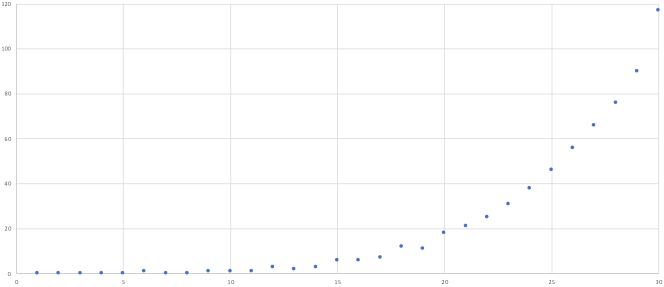
Figure 8: Calculated values of $t_{n}$, $1\leq n\leq 30$.

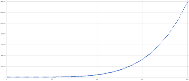
Figure 9: Calculated values of $t_{n}$, $1\leq n\leq 200$.

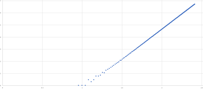
Figure 10: Log-log plot of calculated values of $t_{n}$, $1\leq n\leq 200$.

Figure 11: Calculated values of $t_{n}$, $1\leq n\leq 10000$ (by hundreds).

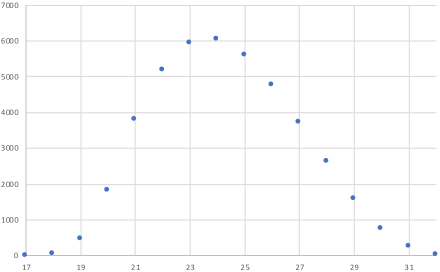
Figure 13: Calculated values of ${}^{d}t_{100}$ (left) and ${}^{d}t_{200}$ (right).

Figure 14: Calculated values of ${}^{d}t_{10000}$ (dark blue) and the discrete derivative (orange). The light blue curve is explained in Section 4.4.

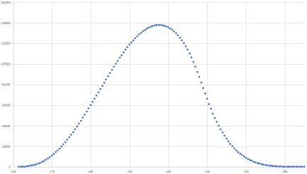
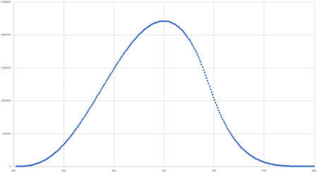
Figure 15: Calculated values of ${}^{50}t_{n}$ (left) and ${}^{100}t_{n}$ (right).

Figure 16: Calculated values of ${}^{1000}t_{n}$ (dark blue) and the discrete derivative (orange). The light blue curve is explained in Section 4.4.

4 Observations from the data

The computational data presented in Section 3 has allowed us to discover some interesting patterns, and has led to a number of natural conjectures, which we discuss in the current section. We do not mean to imply that the following discussion is exhaustive. We hope that other researchers may be able to shed light on some of our conjectures, and make further discoveries.

4.1 Asymptotics

First and foremost, we had hoped that the computed values of $t_{n}$ might have suggested an obvious formula, perhaps after consultation with the OEIS [1]. However, this regrettably was not the case. The “bumpy” nature of the $t_{n}$ sequence, which can be seen in Figure 8, suggests there is no simple formula. However, the sequence does appear to become smoother at a larger scale, as can be seen in Figure 9. This is (apparently) confirmed further in Figure 10, which gives a log-log plot, and suggests a possible power law.

By analogy with the case of triangles, where the answer is asymptotic to $\frac{n^{2}}{48}$ (cf. Honsberger’s Theorem), we might wonder if $t_{n}\sim\frac{n^{k}}{C}$ for some integers $k$ and $C$. If this were so, then

$$\frac{t_{n+1}}{t_{n}}\sim\frac{(n+1)^{k}}{n^{k}}=\frac{n^{k}+kn^{k-1}+\cdots}{n^{k}}\sim 1+\frac{k}{n}.$$

Computed values of $\left(\frac{t_{n+1}}{t_{n}}-1\right)\times n$ strongly suggest a likely value of $k=5$. Computed values of $C_{n}=\frac{n^{5}}{t_{n}}$ suggest a possible value in the order of $C\approx 229000$. Table 6 gives calculated values of $C_{n}$ for $n$ up to $10000$ (by hundreds); Table 7 goes up to $n=20000$ (by thousands). The third column of Table 6 gives the difference $d_{n}=C_{n}-C_{n-100}$, which shows that the fall of $C_{n}$ becomes slower as $n$ increases. The values $d_{n}$ are themselves decreasing, as governed by the ratio $r_{n}=d_{n}/d_{n-100}$. This ratio seems to be tending towards $0.98$ or $0.99$, or thereabouts. If so, then continuing the trend, $C_{n}$ seems to approach $229028$ or $229024$, respectively. So we have the following tentative conjecture; we have made an explicit choice for the denominator so as to have a concrete statement, but there is some level of uncertainty, as just discussed.

Conjecture 4.1.

The number $t_{n}$ of integer tetrahedra of perimeter $n$, up to congruence, satisfies

$$t_{n}\sim\frac{n^{5}}{229024}\qquad\text{as $n\to\infty$.}$$

Taking Conjecture 4.1 as given, one could then aim to analyse the sequence $s_{n}=t_{n}-\frac{n^{5}}{229024}$. For example, one might hope that this is a quartic polynomial. As above, evidence for this could be gathered by calculating values of $\left(\frac{s_{n+1}}{s_{n}}-1\right)\times n$. However, these values appear to be quite chaotic, even when we look at different values of $C$ around the conjectured value of 229024. However, we have more success by splitting up the $s_{n}$ sequence, and looking at subsequences $s_{i},s_{i+k},s_{i+2k},\dots$, for various integers $k\geq 2$ and for each $0\leq i\leq k-1$, especially when $k$ is a multiple of $12$. Here the relevant value to calculate is $\left(\frac{s_{n+k}}{s_{n}}-1\right)\times\frac{n}{k}$, and this does seem to approach $4$ as $n\to\infty$ (for $k\equiv 0\ (\operatorname{mod}12)$), for various $C$. Might there be a multi-case formula for $t_{n}$? Attempts to fit polynomials to subsequences (of the kind described above), using various statistical packages, have not led to any success. In any case, the uncertainty as to the value of $C\approx 229024$ leads to even greater uncertainty here.

Here is an additional note about Conjecture 4.1 (we will return to it again in Section 4.5). Recall that $t_{n}=\frac{1}{24}\sum_{\sigma\in\mathcal{S}_{4}}\operatorname{fix}(\sigma)$; cf. (2.2). For $\sigma\in\mathcal{S}_{4}\setminus\{\operatorname{id}_{4}\}$, it is easy to see that $\operatorname{fix}(\sigma)$ is bounded above by $n^{4}$; this can be seen by examining the constraints on the labels of a graph $G$ fixed by $\sigma$ in cases (ii)–(v), as listed in Section 2. Thus, if $t_{n}$ is indeed (asymptotically) a quintic, then so too is $\operatorname{fix}(\operatorname{id}_{4})=|\mathcal{T}_{n}|$, and so

$$t_{n}\sim\frac{|\mathcal{T}_{n}|}{24}\qquad\text{as $n\to\infty$.}$$

This can be interpreted as saying that virtually all tetrahedra have no symmetry at all. It also leads to an equivalent formulation of Conjecture 4.1, again subject to some uncertainty in the value of the stated numerical coefficient:

Conjecture 4.2.

The set $\mathcal{T}_{n}$ of graphs corresponding to integer tetrahedra of perimeter $n$ satisfies

$$|\mathcal{T}_{n}|\sim\frac{3n^{5}}{28628}\qquad\text{as $n\to\infty$.}$$

Remark 4.3.

Asymptotics of the numbers ${}^{d}t$ were not discussed explicitly by Kurz [12]. However, it was observed on [12, p. 7] that ${}^{d}t$ seems to be approximately $0.103$ times the number of graphs from $\mathcal{G}$ satisfying (T1)^′ and (T2)–(T5); see Proposition 2.5 and Remark 2.13. The language used in [12] was different, and instead spoke of symmetric matrices, but it follows from [12, Lemma 4] that the number of such graphs/matrices is asymptotic to $\frac{d^{5}}{4}$. Thus, a tentative conjecture for an asymptotic expression for ${}^{d}t$ is

$${}^{d}t\sim 0.103\times\frac{d^{5}}{4}\approx\frac{d^{5}}{38.835}\qquad\text{as $d\to\infty$.}$$ (4.4)

This fares quite well with computed values; see Table 8. The non-integrality of the denominator $38.835$ in (4.4) suggests that the denominator in Conjecture 4.1 for the $t_{n}$ sequence might not be an integer either. Again, we will say more about this in Section 4.5.

$n$	$C_{n}$	$d_{n}$	$r_{n}$
$100$	$233552.094$
$200$	$231442.975$	$-2109.119$
$300$	$230489.251$	$-953.724$	$0.452$
$400$	$230045.517$	$-443.734$	$0.465$
$500$	$229786.224$	$-259.293$	$0.584$
$600$	$229619.532$	$-166.692$	$0.643$
$700$	$229509.307$	$-110.225$	$0.661$
$800$	$229428.544$	$-80.763$	$0.733$
$900$	$229367.780$	$-60.765$	$0.752$
$1000$	$229321.619$	$-46.161$	$0.760$
$1100$	$229284.562$	$-37.057$	$0.803$
$1200$	$229255.271$	$-29.291$	$0.790$
$1300$	$229230.648$	$-24.623$	$0.841$
$1400$	$229210.453$	$-20.195$	$0.820$
$1500$	$229193.275$	$-17.179$	$0.851$
$1600$	$229178.649$	$-14.625$	$0.851$
$1700$	$229166.106$	$-12.543$	$0.858$
$1800$	$229155.133$	$-10.973$	$0.875$
$1900$	$229145.626$	$-9.507$	$0.866$
$2000$	$229137.158$	$-8.468$	$0.891$
$2100$	$229129.647$	$-7.511$	$0.887$
$2200$	$229122.995$	$-6.652$	$0.886$
$2300$	$229116.976$	$-6.019$	$0.905$
$2400$	$229111.617$	$-5.359$	$0.890$
$2500$	$229106.724$	$-4.893$	$0.913$
$2600$	$229102.310$	$-4.414$	$0.902$
$2700$	$229098.275$	$-4.035$	$0.914$
$2800$	$229094.575$	$-3.699$	$0.917$
$2900$	$229091.195$	$-3.381$	$0.914$
$3000$	$229088.078$	$-3.116$	$0.922$
$3100$	$229085.208$	$-2.870$	$0.921$
$3200$	$229082.558$	$-2.650$	$0.923$
$3300$	$229080.095$	$-2.463$	$0.929$
$3400$	$229077.802$	$-2.292$	$0.931$
$3500$	$229075.679$	$-2.123$	$0.926$
$3600$	$229073.696$	$-1.982$	$0.934$
$3700$	$229071.831$	$-1.865$	$0.941$
$3800$	$229070.095$	$-1.736$	$0.931$
$3900$	$229068.457$	$-1.637$	$0.943$
$4000$	$229066.931$	$-1.526$	$0.932$
$4100$	$229065.482$	$-1.449$	$0.949$
$4200$	$229064.122$	$-1.360$	$0.939$
$4300$	$229062.837$	$-1.285$	$0.945$
$4400$	$229061.628$	$-1.209$	$0.941$
$4500$	$229060.484$	$-1.144$	$0.946$
$4600$	$229059.392$	$-1.092$	$0.955$
$4700$	$229058.366$	$-1.026$	$0.939$
$4800$	$229057.387$	$-0.979$	$0.955$
$4900$	$229056.459$	$-0.928$	$0.947$
$5000$	$229055.573$	$-0.887$	$0.956$

$n$	$C_{n}$	$d_{n}$	$r_{n}$
$5100$	$229054.729$	$-0.843$	$0.951$
$5200$	$229053.929$	$-0.801$	$0.949$
$5300$	$229053.160$	$-0.768$	$0.960$
$5400$	$229052.428$	$-0.732$	$0.953$
$5500$	$229051.730$	$-0.698$	$0.952$
$5600$	$229051.059$	$-0.672$	$0.963$
$5700$	$229050.420$	$-0.638$	$0.950$
$5800$	$229049.805$	$-0.615$	$0.964$
$5900$	$229049.217$	$-0.588$	$0.956$
$6000$	$229048.654$	$-0.563$	$0.958$
$6100$	$229048.111$	$-0.543$	$0.965$
$6200$	$229047.591$	$-0.520$	$0.956$
$6300$	$229047.090$	$-0.501$	$0.965$
$6400$	$229046.610$	$-0.480$	$0.958$
$6500$	$229046.146$	$-0.464$	$0.965$
$6600$	$229045.700$	$-0.446$	$0.963$
$6700$	$229045.270$	$-0.430$	$0.963$
$6800$	$229044.855$	$-0.415$	$0.965$
$6900$	$229044.455$	$-0.400$	$0.965$
$7000$	$229044.070$	$-0.385$	$0.962$
$7100$	$229043.698$	$-0.373$	$0.968$
$7200$	$229043.339$	$-0.359$	$0.963$
$7300$	$229042.990$	$-0.349$	$0.972$
$7400$	$229042.654$	$-0.337$	$0.966$
$7500$	$229042.329$	$-0.325$	$0.966$
$7600$	$229042.014$	$-0.314$	$0.967$
$7700$	$229041.709$	$-0.306$	$0.972$
$7800$	$229041.413$	$-0.296$	$0.968$
$7900$	$229041.127$	$-0.286$	$0.966$
$8000$	$229040.850$	$-0.277$	$0.969$
$8100$	$229040.580$	$-0.270$	$0.975$
$8200$	$229040.320$	$-0.261$	$0.965$
$8300$	$229040.067$	$-0.253$	$0.971$
$8400$	$229039.821$	$-0.246$	$0.973$
$8500$	$229039.582$	$-0.239$	$0.969$
$8600$	$229039.349$	$-0.233$	$0.978$
$8700$	$229039.124$	$-0.225$	$0.966$
$8800$	$229038.905$	$-0.219$	$0.972$
$8900$	$229038.692$	$-0.213$	$0.974$
$9000$	$229038.485$	$-0.207$	$0.970$
$9100$	$229038.282$	$-0.203$	$0.981$
$9200$	$229038.086$	$-0.196$	$0.965$
$9300$	$229037.895$	$-0.191$	$0.977$
$9400$	$229037.708$	$-0.187$	$0.975$
$9500$	$229037.527$	$-0.181$	$0.970$
$9600$	$229037.350$	$-0.177$	$0.977$
$9700$	$229037.178$	$-0.172$	$0.971$
$9800$	$229037.010$	$-0.168$	$0.979$
$9900$	$229036.846$	$-0.164$	$0.975$
$10000$	$229036.686$	$-0.160$	$0.974$

Table 6: Calculated values of $C_{n}=n^{5}/t_{n}$, and associated differences $d_{n}=C_{n}-C_{n-100}$ and ratios $r_{n}=d_{n}/d_{n-100}$; see Section 4.1 for more details.

4.2 Distributions

Looking at Figures 13 and 14, which graph the numbers ${}^{d}t_{100}$, ${}^{d}t_{200}$ and ${}^{d}t_{10000}$ (for all allowable values of $d$), one sees a general shape emerging. In fact, by plotting scaled graphs of ${}^{d}t_{n}$, one sees that the shapes are essentially identical, up to scale; several such graphs can be seen at [3], including some animations. This means that in principle one might be able to estimate the value of (say) $t_{30000}$ by interpolating the shape of the ${}^{d}t_{30000}$ curve from the ${}^{d}t_{10000}$ or ${}^{d}t_{20000}$ curve (for which we have full data), and calculating a few of the maximum values of ${}^{d}t_{30000}$ to obtain the scaling factor. Table 7 gives the maximum values of ${}^{d}t_{30000}$ and ${}^{d}t_{40000}$, which occur at $d=7140$ and $d=9520$, respectively. The maximum value of ${}^{d}t_{n}$ seems to regularly occur when $d\approx 0.238n\approx\frac{n}{4.2}$. We do not currently know the significance of this number. We will come back to this point in Section 4.5.

Since there are so many points, Figure 14 appears to show a number of continuous curves. The dark blue “curve” plots the sequence ${}^{d}t_{10000}$ ($1667\leq d\leq 3332$), while the orange “curve” is the discrete derivative of this sequence: i.e., the values of ${}^{d}t_{10000}-{}^{d-1}t_{10000}$. (The meaning of the light blue curve will be explained in Section 4.4.) Thus, the orange curve is (an approximation to) the derivative of the blue curve. One may see that although the orange curve appears to be continuous, there is a sharp corner just after the maximum slope (which occurs at around $d=2073$).

Similarly, Figures 15 and 16 graph the numbers ${}^{50}t_{n}$, ${}^{100}t_{n}$ and ${}^{1000}t_{n}$ (for all allowable values of $n$), and again one sees a general shape emerging. Again Figure 16 shows the discrete derivative of the ${}^{1000}t_{n}$ sequence (in orange); although it is not as easy to see, the orange curve also has a sharp corner, this time just before the minimum slope (which occurs at around $n\approx 4830$).

The data used to create Figure 16 also allows one to calculate

$${}^{1000}t=\sum_{n=3003}^{6000}{}^{1000}t_{n}=25728695195597,$$

which agrees with the largest computed value given by Kurz in [12, Table 2]. Some further values of ${}^{d}t$ (up to $d=2000$) are given in Table 8.

4.3 Scratching the surface: maximal diameter

Tables 3 and 4 give values of ${}^{d}t_{n}$, and a couple of simple patterns seem to emerge when looking at the right-most entry of each row, corresponding to the maximum $d$ for a fixed $n$. Specifically, we see the three sequences

$${\color[rgb]{0,0,1}1},{\color[rgb]{0,0,1}1},{\color[rgb]{0,0,1}2},{\color[rgb]{0,0,1}2},{\color[rgb]{0,0,1}3},{\color[rgb]{0,0,1}3},\ldots, {\color[rgb]{.75,.5,.25}0},{\color[rgb]{.75,.5,.25}1},{\color[rgb]{.75,.5,.25}2},{\color[rgb]{.75,.5,.25}3},{\color[rgb]{.75,.5,.25}4},{\color[rgb]{.75,.5,.25}5},\ldots, {\color[rgb]{0,1,0}0},{\color[rgb]{0,1,0}1},{\color[rgb]{0,1,0}3},{\color[rgb]{0,1,0}6},{\color[rgb]{0,1,0}10},{\color[rgb]{0,1,0}13},{\color[rgb]{0,1,0}16},{\color[rgb]{0,1,0}19},{\color[rgb]{0,1,0}22},{\color[rgb]{0,1,0}25},{\color[rgb]{0,1,0}28},{\color[rgb]{0,1,0}31},{\color[rgb]{0,1,0}34},\ldots,$$ (4.5)

corresponding to $$n\equiv 0 n\equiv 1 n\equiv 2\ (\operatorname{mod}3)$$, and , respectively. These are the numbers

$${}^{d}t_{3d+3}\ (d=1,2,3,\ldots), {}^{d}t_{3d+4}\ (d=1,2,3,\ldots), {}^{d}t_{3d+5}\ (d=1,2,3,\ldots),$$

respectively. The apparent patterns in the first two sequences are obvious; it appears that

$${}^{d}t_{3d+3}=\lceil\tfrac{d}{2}\rceil\qquad\text{and}\qquad{}^{d}t_{3d+4}=d-1\qquad\text{for $d\geq 1$.}$$

There are simple explanations for these. We give the details for the first, and sketch them for the second. (We will consider the third sequence later.) We begin with a simple observation:

Lemma 4.6.

Any altitude of an integer triangle is greater than $1/\sqrt{2}$.

Proof.

Let the side-lengths of the triangle be $a\leq b\leq d$, and let $x$ be any of $a,b,d$. Let $h$ be the altitude measured from a side of length $x$, and denote the area of the triangle by $A=xh/2$. By Heron’s formula, and keeping $a\leq b\leq d$ and $a+b\geq d+1$ in mind, we have

$$h^{2}=\frac{4A^{2}}{x^{2}}\geq\frac{4A^{2}}{d^{2}} =\frac{4}{d^{2}}\cdot\frac{1}{16}\cdot(a+b+d)\cdot(a+b-d)\cdot(a-b+d)\cdot(-a+b+d)$$

$$\geq\frac{1}{4d^{2}}\cdot(2d+1)\cdot 1\cdot a\cdot d>\frac{2ad^{2}}{4d^{2}}=\frac{a}{2}\geq\frac{1}{2}.$$

The result follows. ∎

Remark 4.7.

If the shortest side of an integer triangle is at least $2$, then it follows from the above proof that any altitude is greater than $1$. Of course this is not true if the shortest side has length $1$, and if the altitude is measured from one of the two sides of length $d$; in fact it is easy to show that $h^{2}=1-1/4d^{2}$ in this case. Since the latter is decreasing in $d$, and equal to $3/4$ when $d=1$, the lower bound of $1/\sqrt{2}\approx 0.707$ in Lemma 4.6 could be replaced by $\sqrt{3}/2\approx 0.866$, though the latter is not a strict lower bound.

Lemma 4.8.

For any $d\geq 1$ we have ${}^{d}t_{3d+3}=\lceil\tfrac{d}{2}\rceil$.

Proof.

First consider an integer triangle with side-lengths $B\leq C\leq d$ satisfying ${B+C=d+1}$, and join two copies of this triangle together in the way shown in Figure 20. By Lemma 4.6, we can fold these towards each other (as in Figure 6) until the tips are $1$ unit apart, thus obtaining an integer tetrahedron of diameter $d$ and perimeter $3d+3$. There are $\lceil\tfrac{d}{2}\rceil$ such triangles, and they give rise to pairwise-noncongruent tetrahedra.

Conversely, let $T$ be an arbitrary tetrahedron with diameter $d$ and perimeter $n=3d+3$. We can construct $T$ by folding, as in Figure 6, assuming that $A=d$ and $B\leq C$. To ensure that $n=3d+3$ we must of course have $B+C=b+c=d+1$ and $a=1$. To complete the proof, we must show that $B=c$, as then also $C=b$. Aiming for a contradiction, suppose instead that $B\not=c$, and consider the points $P$ and $Q$ as shown in Figure 6. These are on the circles $x^{2}+y^{2}=B^{2}$ and $x^{2}+y^{2}=c^{2}$, respectively. Since $B$ and $c$ differ by at least $1$ (as they are distinct positive integers), it follows that $|PQ|\geq 1=a$. But this contradicts $|PQ|<a<|PR|$ from the proof of Proposition 2.5. ∎

Figure 20: Creating an integer tetrahedron of diameter $d$ and perimeter $n=3d+3$ by folding congruent triangles (with $B+C=d+1$); see the proof of Lemma 4.8 for more details, and cf. Figure 6.

Lemma 4.9.

For any $d\geq 1$ we have ${}^{d}t_{3d+4}=d-1$.

Sketch of proof..

Again we must analyse the pairs of triangles $(B,C,d)$ and $(b,c,d)$ that can be folded to create appropriate tetrahedra, as in Figure 6 (with $A=d$). Up to symmetry, this time we have either

1. $B+C=b+c=d+1$ and $a=2$, or else

2. $B+C=d+1$, $b+c=d+2$ and $a=1$.

We first note that case (b) never actually occurs. Indeed, here, since $B+C\not=b+c$, we must either have $B\not=c$ or $C\not=b$ (or both). Considering circles, as in the proof of Lemma 4.8, we see that $|PQ|\geq 1=a$, so the folding procedure cannot be carried out.

This leaves us to consider case (a), and we assume without loss of generality that $B\leq c$. Again considering circles, $B$ and $c$ cannot differ by more than $1$, so we must have either

1. $c=B$ (and $b=C$), or else

2. $c=B+1$ (and $b=C-1$).

We consider these in turn, and show that there are $\lceil\tfrac{d}{2}\rceil-1$ and $\lfloor\tfrac{d}{2}\rfloor$ tetrahedra in each case. Since these sum to $d-1$, this will complete the proof.

(a1). By symmetry, we may also assume that $B\leq C(=d+1-B)$. So $1\leq B\leq\lceil\tfrac{d}{2}\rceil$. Using Remark 4.7, we see that the folding procedure can be carried out in every case except for $B=1$.

(a2). We again have $1\leq B\leq\lceil\tfrac{d}{2}\rceil$, and this time the folding procedure can be carried out in each case. However, when $d$ is odd, the $B=\lceil\tfrac{d}{2}\rceil-1$ and $B=\lceil\tfrac{d}{2}\rceil$ cases produce congruent tetrahedra. So we obtain $\tfrac{d}{2}$ tetrahedra when $d$ is even, and $\lceil\tfrac{d}{2}\rceil-1$ when $d$ is odd. In both cases, this is equal to $\lfloor\tfrac{d}{2}\rfloor$. ∎

The behaviour of the third sequence in (4.5) appears to be rather more complex. For convenience in the following discussion, we will write ${u_{d}={}^{d}t_{3d+5}}$ for $d\geq 1$. While these numbers seem to quickly stabilise into an arithmetic progression, $u_{d}=3d-5$ ($d\geq 5$), this only persists until $d=41$, where we see an interesting change in the sequence:

$$\ldots,{\color[rgb]{0,1,0}100},{\color[rgb]{0,1,0}103},{\color[rgb]{0,1,0}106},{\color[rgb]{0,1,0}109},{\color[rgb]{0,1,0}112},{\color[rgb]{0,1,0}115},{\color[rgb]{0,1,0}118},{\color[rgb]{1,0,0}\bf 115},{\color[rgb]{1,0,0}\bf 115},{\color[rgb]{1,0,0}\bf 116},{\color[rgb]{1,0,0}\bf 117},{\color[rgb]{1,0,0}\bf 118},{\color[rgb]{1,0,0}\bf 119},{\color[rgb]{1,0,0}\bf 121},{\color[rgb]{1,0,0}\bf 122},{\color[rgb]{1,0,0}\bf 124},{\color[rgb]{1,0,0}\bf 126},{\color[rgb]{1,0,0}\bf 127},{\color[rgb]{1,0,0}\bf 129},\ldots$$

The colours in the above lists are reflected in Tables 3 and 4, and we note that $u_{41}={\color[rgb]{0,1,0}118}$ and $u_{42}={\color[rgb]{1,0,0}\bf 115}$. The sequence of differences $u_{d+1}-u_{d}$ ($d\geq 42$) begins

$$0,1,1,1,1,2,1,2,2,1,2,2,1,2,2,2,1,2,2,2,2,2,2,1,2,2,2,2,2,2,2,2,1,\ldots.$$

Although this appears somewhat chaotic, further calculations show that the last difference of $1$ seems to occur at $d=1110$, with all subsequent differences being $2$. See Figure 21, which plots the differences $u_{d+1}-u_{d}$ (right), and also the ratios $u_{d}/d$ (left). The above discussion suggests the possible formula

$$u_{d}={}^{d}t_{3d+5}=2d+15\qquad\text{for $d\geq 1111$.}$$ (4.10)

We have verified this computationally up to $d=50,000,000$. Interestingly, we obtained much better performance using the “naïve” algorithm described in Section 3.1 (see steps (I)–(IV)), as compared to our modification of Kurz’s algorithm from [12]. (For example, the latter calculated $u_{3000}=6015$ in around 2 hours, while the former took a fraction of a second; it calculated the $50,000,000$th term in around 80 minutes.) The reason for this appears to be that our original algorithm directly creates and stores all tetrahedra with given dimensions, and then counts them; this led to serious memory issues in general, but for parameters $n,d$ for which ${}^{d}t_{n}$ is relatively small (such as $n=3d+5$) this is actually an advantage. As discussed in Section 3.1, the Kurz-based algorithm moves through tuple space, counting or rejecting tuples as appropriate; it seems that when $n$ is small relative to $d$, many more tuples are rejected than counted, leading to longer running times.

We have not attempted to prove (4.10), but we expect this could be done (if it is true) in a similar way to Lemmas 4.8 and 4.9 above. Computations suggest that for $d\geq 1111$, there are:

• $\lfloor\tfrac{d}{2}\rfloor-1$ tetrahedra with $a=1$,

• $\lceil\tfrac{3d}{2}\rceil-3$ tetrahedra with $a=3$, and

• $19$ “sporadic” tetrahedra with $a=2$,

and these sum to $2d+15$. For smaller $d$ the number of sporadic tetrahedra is different; for example, it is $20$ for $205\leq d\leq 1110$. Figure 22 plots the number of such sporadic tetrahedra for $1\leq d\leq 2000$.

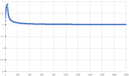
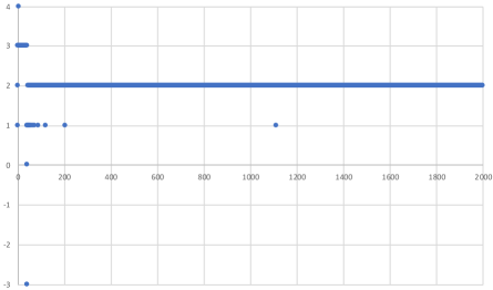
Figure 21: Left and right: calculated values of $u_{d}/d$ and $u_{d+1}-u_{d}$, $1\leq d\leq 2000$, where $u_{d}={}^{d}t_{3d+5}$.

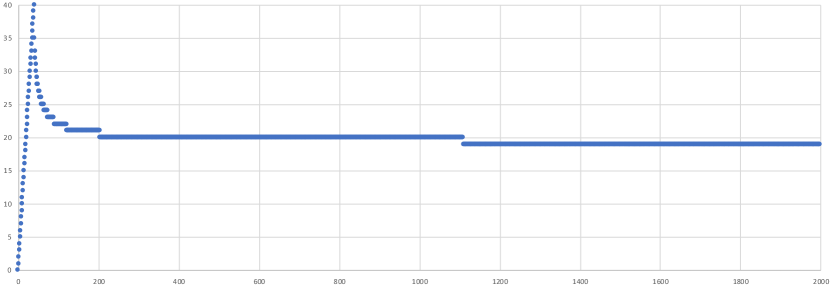
Figure 22: The number of “sporadic” tetrahedra with diameter $d$ and perimeter $3d+5$, $1\leq d\leq 2000$; see Section 4.3 for more details.

We have not attempted to systematically study the numbers ${}^{d}t_{3d+k}$ for (fixed) $k\geq 6$, but Figure 23 gives some graphs of computed values for $k=3,4,\ldots,10$. It appears that for fixed $k$, the sequence ${}^{d}t_{3d+k}$ ($d=1,2,3,\ldots$) is eventually linear in $d$, but the “pre-linear” behaviour becomes more complex, and lasts longer as $k$ increases. Taking $k=10$, for example, and writing $v_{d}={}^{d}t_{3d+10}$, Figure 24 shows the ratios $v_{d}/d$ and differences $v_{d+1}-v_{d}$ (cf. Figure 21, which does the same for $k=5$). Both appear to approach a limit of $10$, strongly suggesting that eventually $v_{d}=10d+l$ for some $l$. Calculations suggest that $l=2470$; this value of $l$ holds for $2,000,000\leq d\leq 20,000,000$. But we note that $l=2471$ for $d=1,000,000$, so that the “pre-linear” behaviour persists beyond the $1,000,000$th term.

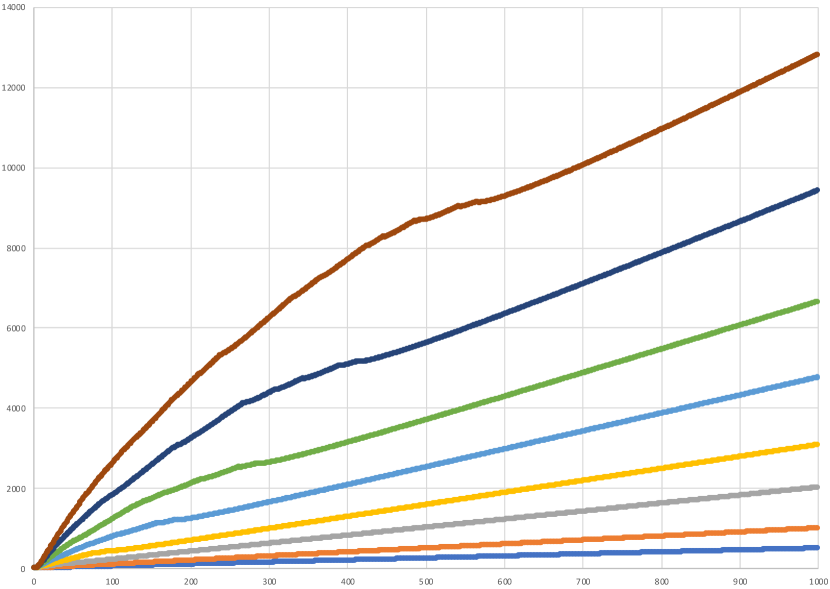
Figure 23: Calculated values of ${}^{d}t_{3d+k}$, $1\leq d\leq 1000$, for $k=3,4,\ldots,10$ (bottom to top).

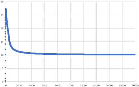
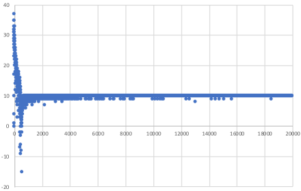
Figure 24: Left and right: calculated values of $v_{d}/d$ and $v_{d+1}-v_{d}$, $1\leq d\leq 20000$, where $v_{d}={}^{d}t_{3d+10}$.

4.4 Initial segments: a glimpse of order and hope?

In the previous section we looked at the very top parts of the columns in the ${}^{d}t_{n}$ data, as shown in Tables 3 and 4. One of the most interesting/promising observations arises when one looks at the bottom parts of these columns.

Examining consecutive columns, one sees that the first few values at the bottom of one column are present in the next. These are the red entries in the lower parts of Tables 3 and 4, specifically the values ${}^{d}t_{n}$ with $n$ approximately ranging from $5d$ to $6d$. Note that each column seems to add an extra number to the “Stable Column Sequence” (as we will call it), but that no extra number is added from column $d=28$ to $d=29$; this is indicated by green in Table 4. Although we do not have a complete explanation for why this happens, it appears that for fixed $d$, the last value of $n$ for which ${}^{d}t_{n}$ is not this “stable” value is $\lceil 5.035d\rceil$; note that

$$\lceil 5.035\cdot 28\rceil=\lceil 140.98\rceil=141\qquad\text{and}\qquad\lceil 5.035\cdot 29\rceil=\lceil 146.015\rceil=147,$$

so that column $d=29$ adds an additional $6$ “unstable” ${}^{d}t_{n}$ values from column $d=28$.

In any case, the resulting Stable Column Sequence begins:

$$1,1,3,6,11,18,31,47,72,105,149,206,281,372,487,627,796,997,1237,1516,1843,2220,2653,3147,\ldots$$ (4.11)

This sequence does not appear on the OEIS. The first few values are easy to understand:

• for $d\geq 1$, ${}^{d}t_{6d}=1$ counts only $\big{[}(d,d),(d,d),(d,d)\big{]}$, the equilateral tetrahedron,

• for $d\geq 2$, ${}^{d}t_{6d-1}=1$ counts only $\big{[}(d,d),(d,d),(d,d-1)\big{]}$,

• for $d\geq 3$, ${}^{d}t_{6d-2}=3$ counts only $\big{[}(d,d),(d,d),(d,d-2)\big{]}$, $\big{[}(d,d),(d,d),(d-1,d-1)\big{]}$ and $\big{[}(d,d),(d,d-1),(d,d-1)\big{]}$.

One could similarly explain other values, with ad hoc arguments: e.g., ${}^{d}t_{6d-3}=6$ for $d\geq 4$.

If we denote the sequence (4.11) by $a_{k}$ ($k=0,1,2,\ldots$), then calculating $\left(\frac{a_{k+1}}{a_{k}}-1\right)\times k$ suggests that $a_{k}$ is quartic in $k$. Further experimentation quickly suggests the leading coefficient is $\frac{1}{96}$. Additional analysis suggests that $a_{k}-\frac{k^{2}}{96}$ is quadratic with leading coefficient $\frac{7}{16}=\frac{42}{96}$. After examining $a_{k}-\frac{k^{4}}{96}-\frac{7k^{2}}{16}$, it eventually appears that we have the exact formula

$$a_{k}=\frac{k^{4}+42k^{2}+b_{k}}{96}\qquad\text{where $b_{0}=96$, and for $k\geq 1$:}\qquad b_{k}=\begin{cases}192&\text{if $k\equiv 0\ (\operatorname{mod}12)$}\\ 53&\text{if $k\equiv 1,5,7,11\ (\operatorname{mod}12)$}\\ 104&\text{if $k\equiv 2,10\ (\operatorname{mod}12)$}\\ 117&\text{if $k\equiv 3,9\ (\operatorname{mod}12)$}\\ 128&\text{if $k\equiv 4,8\ (\operatorname{mod}12)$}\\ 168&\text{if $k\equiv 6\ (\operatorname{mod}12)$.}\end{cases}$$ (4.12)

Equivalently, for $k\geq 1$, $a_{k}$ is the nearest integer to

$$\frac{k^{4}+42k^{2}+148}{96}\qquad\text{or}\qquad\frac{k^{4}+42k^{2}+85}{96},$$

for even and odd $k$, respectively. (The values of $148$ and $85$ are simply the average of the maximum and minimum values of $b_{k}$ for even and odd $k$, respectively. A single “nearest integer formula” cannot be given, unfortunately, because the distance between the maximum and minimum values of $b_{k}$ for arbitrary $k$ (i.e., $192-53=139$) is greater than the denominator, $96$.) We do not currently know if there is any significance in the exact values of the numbers $b_{k}\in\{53,104,117,128,168,192\}$.

Conjecture 4.13.

For suitably small $k$ (approximately $0\leq k<d$), we have ${}^{d}t_{6d-k}=a_{k}$, where $a_{k}$ is defined in (4.12). (Note then that for such $k$, ${}^{d}t_{6d-k}$ would depend only on $k$, and not on $d$.)

The formula (4.12) can be used to calculate many more values of $a_{k}$. Figure 25 plots these, together with the associated values of $b_{k}$; the periodic nature of the latter can be readily seen in the graph.

The existence of the Stable Column Sequence implies that there are six “Stable Row Sequences”, one for each residue of $n$, modulo $6$. So the $n$th row of the ${}^{d}t_{n}$ table, for suitably large $n$, begins:

• $18,206,997,3147,7736,16168,30171,51797,83422,\ldots$ when $n\equiv 0\ (\operatorname{mod}6)$,

• $11,149,796,2653,6747,14427,27368,47567,77347,\ldots$ when $n\equiv 1\ (\operatorname{mod}6)$,

• $6,105,627,2220,5856,12831,24765,43602,71610,\ldots$ when $n\equiv 2\ (\operatorname{mod}6)$,

• $3,72,487,1843,5057,11372,22353,39891,66199,\ldots$ when $n\equiv 3\ (\operatorname{mod}6)$,

• $1,47,372,1516,4343,10041,20122,36422,61101,\ldots$ when $n\equiv 4\ (\operatorname{mod}6)$,

• $1,31,281,1237,3710,8833,18065,33187,56306,\ldots$ when $n\equiv 5\ (\operatorname{mod}6)$.

These can all be seen in Table 4, and they are all of course subsequences of the Stable Column Sequence. None of these six (sub)sequences appear on the OEIS. Note that the (initial segments of the) Stable Row Sequences account for the left-most part of the graphs in Figures 13 and 14; see especially Figure 14, which shows values of $a_{k}$ in light blue. Similarly, the Stable Column Sequence accounts for the right-most part of the graphs in Figures 15 and 16; see especially Figure 16, which shows values of $a_{k}$ in light blue.

So we have seen that the first portion of a row, and the last portion of a column, in the ${}^{d}t_{n}$ table appears to be governed by a certain quartic (indeed, biquadratic) polynomial. Unfortunately, similar experimentation shows that the remainder of these rows/columns do not look at all like any polynomial. Indeed, even considering small portions at the opposite end of each row/column does not seem to yield a polynomial pattern.

A possible approach to Conjecture 4.13 might be to show that any tuple $\big{[}(A,a),(B,b),(C,c)\big{]}$ with $d=A=\max\{A,B,C,a,b,c\}$, and with perimeter greater than (around) $5.035d$, automatically satisfies conditions (T2)–(T6) from Proposition 2.5. The hope is that such a tuple is “close enough” to the equilateral $\big{[}(d,d),(d,d),(d,d)\big{]}$ that it corresponds to a tetrahedron by default. This would not immediately give the desired formula for $a_{k}$, but it would at least show that some kind of Stable Column Sequence does exist.

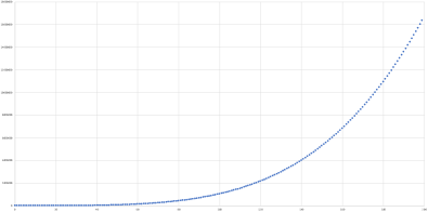
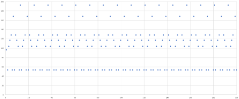
Figure 25: Calculated values of $a_{k}$ (left) and $b_{k}$ (right), $1\leq k\leq 200$, as defined in (4.12).

4.5 Sums vs. maximums: more on asymptotics

We noted in Section 4.2 that one might hope to approximate values of $t_{n}$ (for large $n$) by interpolating the ${}^{d}t_{m}$ curve (for smaller $m$), and using the value of $\max_{d}{}^{d}t_{n}$ as the scaling factor. In this section we discuss a simpler attempt to estimate $t_{n}$ (and ${}^{d}t$) using single values of ${}^{d}t_{n}$.

To keep the following discussion manageable, it will be convenient to define a number of additional parameters:

• For fixed $n$ we define $\mu_{n}=\max_{d}{}^{d}t_{n}$, and the ratio $\rho_{n}=t_{n}/\mu_{n}$.
  Further, let $d^{*}(n)$ be the diameter corresponding to the maximum value of ${}^{d}t_{n}$: i.e., $\mu_{n}={}^{d^{*}(n)}t_{n}$.

• For fixed $d$ we define ${}^{d}\!\mu=\max_{n}{}^{d}t_{n}$, and the ratio ${}^{d}\!\rho={}^{d}t/{}^{d}\!\mu$.
  Further, let $n^{*}(d)$ be the perimeter corresponding to the maximum value of ${}^{d}t_{n}$: i.e., ${}^{d}\!\mu={}^{d}t_{n^{*}(d)}$.

Computationally, it seems that

$$d^{*}(n)\approx 0.238n\approx\frac{n}{4.2}\qquad\text{and}\qquad n^{*}(d)\approx 4.5d.$$ (4.14)

We do not currently understand the significance of the number $0.238\approx\frac{1}{4.2}$. However, $4.5d$ is of course almost exactly mid-way between the extreme values of $3d+3\leq n\leq 6d$; cf. Lemma 3.2. These values of $d^{*}(n)$ and $n^{*}(d)$ can be seen by locating the peaks in Figures 13–16.

Figure 26 shows graphs of calculated values of $\rho_{n}$ ($n\leq 2000$) and ${}^{d}\!\rho$ ($d\leq 300$). These graphs strongly suggest that (at least approximately) $\rho_{n}$ is linear in $n$, and ${}^{d}\!\rho$ is linear in $d$, so it seems worthwhile to look at the values of $\rho_{n}/n$ and ${}^{d}\!\rho/d$. Accordingly,

• Table 7 shows calculated values of $t_{n}$, $\mu_{n}$, $\rho_{n}$ and $\rho_{n}/n$ (as well as $d^{*}(n)$), and

• Table 8 shows calculated values of ${}^{d}t$, ${}^{d}\!\mu$, ${}^{d}\!\rho$ and ${}^{d}\!\rho/d$ (as well as $n^{*}(d)$).

Note that we have been able to calculate $\mu_{n}$ and ${}^{d}\!\mu$ for higher values of $n$ and $d$ than for $t_{n}$ and ${}^{d}t$. To obtain these we used the approximations for $d^{*}(n)$ and $n^{*}(d)$ from (4.14), and calculated enough values of ${}^{d}t_{n}$ around the critical values, to ensure that we had found the peak of the curve. For the round values of $n$ and $d$ we used, the approximations in (4.14) were in fact exact, with a single exception: $n^{*}(1900)=8551$, whereas $4.5\cdot 1900=8550$. But here we note that

• ${}^{1900}t_{8549}=287666266084$,

• ${}^{1900}t_{8550}=287666506644={}^{1900}t_{8549}+240560$,

• ${}^{1900}t_{8551}=287666521356={}^{1900}t_{8550}+14712$,

• ${}^{1900}t_{8552}=287666235410={}^{1900}t_{8551}+271234$,

meaning that ${}^{1900}t_{8550}$ is comparatively very close to the maximum value of ${}^{1900}\mu={}^{1900}t_{8551}$.

The values displayed in Tables 7 and 8 strongly suggest that $\rho_{n}/n$ and ${}^{d}\!\rho/d$ tend to limits of around $0.07122$ and $1.1657$, respectively, leading to asymptotic expressions:

$$\rho_{n}\sim 0.07122n\text{ \ as $n\to\infty$}\qquad\text{and}\qquad{}^{d}\!\rho\sim 1.1657d\text{ \ as $d\to\infty$.}$$ (4.15)

(Interestingly, $0.07122$ is quite close to $\frac{1}{14}$, although computational evidence suggests that the limit $\lim_{n\to\infty}\frac{\rho_{n}}{n}$ is around $\frac{1}{14.041}$, and this can make quite a big difference in the calculations that follow.)

By definition, we have $t_{n}=\rho_{n}\times\mu_{n}$ and ${}^{d}t={}^{d}\!\rho\times{}^{d}\!\mu$. Thus, if we could also obtain asymptotic expressions for $\mu_{n}$ and ${}^{d}\!\mu$, then these could be combined with (4.15) to yield asymptotic expressions for $t_{n}$ and ${}^{d}t$ themselves (cf. Conjecture 4.1 and Remark 4.3).

Calculations show that the ratios $\left(\frac{\mu_{n+1}}{\mu_{n}}-1\right)\times n$ and $\left(\frac{{}^{d+1}\mu}{{}^{d}\!\mu}-1\right)\times d$ both seem to approach $4$, suggesting that $\mu_{n}\sim\frac{n^{4}}{D}$ and ${}^{d}\!\mu\sim\frac{d^{4}}{E}$ for some constants $D$ and $E$. Tables 7 and 8 also show values of $D_{n}=\frac{n^{4}}{\mu_{n}}$ and ${}^{d}D=\frac{d^{4}}{{}^{d}\!\mu}$, respectively. (These tables also give values of $C_{n}=\frac{n^{5}}{t_{n}}$ and ${}^{d}C=\frac{d^{5}}{{}^{d}t}$.) These seem to approach limits of around $D_{n}\to 16310.5$ and ${}^{d}D\to 45.301$, respectively.

Putting all of the above together, we have (very approximate) candidates for asymptotic formulas:

$$t_{n} =\rho_{n}\times\mu_{n}\sim 0.07122n\times\frac{n^{4}}{16310.5}\approx\frac{n^{5}}{229016} n\to\infty$$ as (4.16)

$$\text{and}\qquad\qquad{}^{d}t ={}^{d}\!\rho\times{}^{d}\!\mu\sim 1.1657d\times\frac{d^{4}}{45.301}\approx\frac{d^{5}}{38.86} d\to\infty$$ as . (4.17)

Note that (4.16) and (4.17) are reasonably close to Conjecture 4.1 and (4.4). We should stress, however, that in the above discussion we often rounded off certain numbers to seemingly-arbitrary precision. Thus, the asymptotic expressions in (4.16) and (4.17) are very speculative, and are not meant to be exact predictions.

Figure 26: Calculated values of $\rho_{n}$ (left), $1\leq n\leq 2000$, and ${}^{d}\!\rho$ (right), $1\leq d\leq 300$; see Section 4.5 for more details.

$n$	$d^{*}(n)$	$t_{n}$	$\mu_{n}$	$\rho_{n}$	$\rho_{n}/n$	$D_{n}$	$C_{n}$
$1000$	$238$	$4360687860$	$61261647$	$71.181368$	$0.071181368$	$16323.42663$	$229321.6190$
$2000$	$476$	$139654346301$	$980662960$	$142.408097$	$0.071204049$	$16315.49335$	$229137.1579$
$3000$	$714$	$1060727392377$	$4965253737$	$213.630048$	$0.071210016$	$16313.36570$	$229088.0784$
$4000$	$952$	$4470309160343$	$15693529026$	$284.850473$	$0.071212618$	$16312.45589$	$229066.9310$
$5000$	$1190$	$13642977397892$	$38315438250$	$356.069982$	$0.071213996$	$16311.96271$	$229055.5726$
$6000$	$1428$	$33949118928429$	$79452345303$	$427.289072$	$0.071214845$	$16311.66450$	$229048.6541$
$7000$	$1666$	$73378891579018$	$147197080983$	$498.507790$	$0.071215399$	$16311.46477$	$229044.0703$
$8000$	$1904$	$143066182224551$	$251113882084$	$569.726297$	$0.071215787$	$16311.32443$	$229040.8501$
$9000$	$2142$	$257812568218126$	$402238432945$	$640.944641$	$0.071216071$	$16311.22106$	$229038.4849$
$10000$	$2380$	$436611276762080$	$613077830990$	$712.162885$	$0.071216288$	$16311.14272$	$229036.6862$
$11000$	$2618$	$703171140799375$	$897610575535$	$783.381079$	$0.071216462$	$16311.08233$	$229035.2813$
$12000$	$2856$	$1086440561201385$	$1271286727639$	$854.599153$	$0.071216596$	$16311.03318$	$229034.1588$
$13000$	$3094$	$1621131464654093$	$1751027590016$	$925.817202$	$0.071216708$	$16310.99371$	$229033.2450$
$14000$	$3332$	$2348243259709892$	$2355226146934$	$997.035152$	$0.071216797$	$16310.96022$	$229032.4896$
$15000$	$3570$	$3315586803814407$	$3103746427345$	$1068.253120$	$0.071216875$	$16310.93299$	$229031.8562$
$16000$	$3808$	$4578308347767338$	$4017924323570$	$1139.471025$	$0.071216939$	$16310.90950$	$229031.3191$
$17000$	$4046$	$6199413506818430$	$5120566904917$	$1210.688899$	$0.071216994$	$16310.88931$	$229030.8589$
$18000$	$4284$	$8250291212969114$	$6435952631653$	$1281.906764$	$0.071217042$	$16310.87207$	$229030.4610$
$19000$	$4522$	$10811237680756863$	$7989831502801$	$1353.124616$	$0.071217085$	$16310.85711$	$229030.1141$
$20000$	$4760$	$13971980347794463$	$9809425098449$	$1424.342427$	$0.071217121$	$16310.84374$	$229029.8097$
$30000$	$7140$		$49660446083302$			$16310.76770$
$40000$	$9520$		$156951842767924$			$16310.78743$

Table 7: Calculated values of $t_{n}$ and associated numbers defined in Section 4.5.

$d$	$n^{*}(d)$	${}^{d}t$	${}^{d}\!\mu$	${}^{d}\!\rho$	${}^{d}\!\rho/d$	${}^{d}D$	${}^{d}C$
$100$	$450$	$256866619$	$2205518$	$116.465438$	$1.164654376$	$45.34082243$	$38.93071057$
$200$	$900$	$8227353208$	$35302466$	$233.053215$	$1.165266076$	$45.32261287$	$38.89464715$
$300$	$1350$	$62496428392$	$178753878$	$349.622784$	$1.165409278$	$45.31370223$	$38.88222195$
$400$	$1800$	$263399396125$	$564995595$	$466.197256$	$1.165493140$	$45.31008777$	$38.87632299$
$500$	$2250$	$803900006590$	$1379446698$	$582.769894$	$1.165539789$	$45.30802103$	$38.87299383$
$600$	$2700$	$2000468396580$	$2860504080$	$699.341214$	$1.165568690$	$45.30669993$	$38.87089650$
$700$	$3150$	$4323958989350$	$5299548768$	$815.910784$	$1.165586834$	$45.30574404$	$38.86947134$
$800$	$3600$	$8430487428682$	$9040920238$	$932.481120$	$1.165601400$	$45.30512262$	$38.86845248$
$900$	$4050$	$15192308794063$	$14481975268$	$1049.049492$	$1.165610546$	$45.30459332$	$38.86769338$
$1000$	$4500$	$25728695195597$	$22072986511$	$1165.619124$	$1.165619124$	$45.30424551$	$38.86710898$
$1100$	$4950$	$41436812404716$	$32317280628$	$1282.187474$	$1.165624976$	$45.30393559$	$38.86664795$
$1200$	$5400$	$64022597756042$	$45771110797$	$1398.755605$	$1.165629670$	$45.30368531$	$38.86627671$
$1300$	$5850$	$95531638650235$	$63043701776$	$1515.324068$	$1.165633899$	$45.30349455$	$38.86597207$
$1400$	$6300$	$138380047521949$	$84797295248$	$1631.892233$	$1.165637310$	$45.30333177$	$38.86571870$
$1500$	$6750$	$195385341804382$	$111747102464$	$1748.460027$	$1.165640018$	$45.30318808$	$38.86550511$
$1600$	$7200$	$269797320709960$	$144661271196$	$1865.027996$	$1.165642497$	$45.30307211$	$38.86532295$
$1700$	$7650$	$365328940733369$	$184360988174$	$1981.595696$	$1.165644527$	$45.30296828$	$38.86516620$
$1800$	$8100$	$486187194335920$	$231720360895$	$2098.163461$	$1.165646367$	$45.30288128$	$38.86503022$
$1900$	$8551$	$637103991780086$	$287666521356$	$2214.731102$	$1.165647948$	$45.30280388$	$38.86491110$
$2000$	$9000$	$823367026746276$	$353179561833$	$2331.298625$	$1.165649312$	$45.30273472$	$38.86480629$
$3000$	$13501$		$1787987440725$			$45.30233164$
$4000$	$18001$		$5650944679691$			$45.30215999$
$5000$	$22501$		$13796279726716$			$45.30206783$
$6000$	$27001$		$28608001167605$			$45.30201157$
$7000$	$31502$		$52999897734423$			$45.30197420$

Table 8: Calculated values of ${}^{d}t$ and associated numbers defined in Section 4.5.

5 Conclusion

Enumeration of integer triangles of given perimeter is a classical problem [11, 8], and polygons have recently been treated as well [4]. The current article considered the corresponding problem for tetrahedra, which is considerably more difficult. The central theme is the calculation of the numbers $t_{n}$, ${}^{d}t$ and ${}^{d}t_{n}$ of integer tetrahedra with perimeter $n$ and/or diameter $d$ (as appropriate), up to congruence. In Section 2 we set up a framework in which these numbers could (in principle) be calculated via an application of Burnside’s Lemma, and made some partial progress by finding explicit formulas for some of the relevant fix-set parameters. The complexity of the other parameters—and of the numbers $t_{n}$, ${}^{d}t$ and ${}^{d}t_{n}$ themselves—is highlighted by the computations discussed in Section 3, and is visible in many of the figures therein. Nevertheless, a number of apparent patterns emerged from an exploration of the data. Several of these were discussed in Section 4, which contains a number of conjectures and avenues for future exploration; we hope that future studies will shed further light on the situation.

References

- [1] The on-line encyclopedia of integer sequences. Published electronically at http://oeis.org/.
- [2] P. J. Cameron. Combinatorics: topics, techniques, algorithms. Cambridge University Press, Cambridge, 1994.
- [3] J. East, M. Hendriksen, and L. Park. On the enumeration of integer tetrahedra: supplemental data, 2021, https://staff.cdms.westernsydney.edu.au/~lapark/integer_tetrahedra/.
- [4] J. East and R. Niles. Integer polygons of given perimeter. Bull. Aust. Math. Soc., 100(1):131–147, 2019.
- [5] J. East and R. Niles. Integer triangles of given perimeter: a new approach via group theory. Amer. Math. Monthly, 126(8):735–739, 2019.
- [6] M. D. Hirschhorn. Triangles with integer sides, revisited. Math. Mag., 73(1):53–56, 2000.
- [7] M. D. Hirschhorn. Triangles with integer sides. Math. Mag., 76(4):306–308, 2003.
- [8] R. Honsberger. Mathematical gems. III, volume 9 of The Dolciani Mathematical Expositions. Mathematical Association of America, Washington, DC, 1985.
- [9] J. E. Humphreys. Reflection groups and Coxeter groups, volume 29 of Cambridge Studies in Advanced Mathematics. Cambridge University Press, Cambridge, 1990.
- [10] T. Jenkyns and E. Muller. Triangular triples from ceilings to floors. Amer. Math. Monthly, 107(7):634–639, 2000.
- [11] J. H. Jordan, R. Walch, and R. J. Wisner. Triangles with integer sides. Amer. Math. Monthly, 86(8):686–689, 1979.
- [12] S. Kurz. Enumeration of integral tetrahedra. J. Integer Seq., 10(9):Article 07.9.3, 12, 2007.
- [13] K. Menger. Untersuchungen über allgemeine Metrik. Math. Ann., 100(1):75–163, 1928.
- [14] K. Wirth and A. S. Dreiding. Edge lengths determining tetrahedrons. Elem. Math., 64(4):160–170, 2009.