On disc-with-hole and disc-with-handle partition functions in bosonic string theory

Abstract

Higher genus partition functions of string world sheets with boundaries are relevant, e.g. for computation of quantum corrections to Wilson loop expectation values. As a preparation for a possible study of strings in curved space like AdS here we consider examples of genus one partition functions of string world-sheets ending on a circle in the bosonic string theory in flat space. We begin with the partition function for annular topology, writing it as an integral over the modulus of the annulus. In the process, we compute the determinant of the Laplacian on the annulus for Dirichlet-Dirichlet and Dirichlet-Neumann boundary conditions. We then consider the case of the disc-with-handle topology using the gluing method. We first write the partition function using a Schottky parameterisation of the moduli space and then as an integral over the period matrix.

Presented here is joint work done by the authors towards theses submitted in partial fulfillment of the requirements for the MSci degree in Physics with Theoretical Physics of Imperial College London.

1 Introduction

The correspondence between Wilson loops (WLs) in large $N$ $\mathcal{N}=4$ SYM gauge theory and partition functions of $AdS_{5}\times S^{5}$ string world-sheets ending on a fixed curve has been heavily studied since PhysRevLett.80.4859 ; PhysRevD.60.125006 . A systematic discussion of leading string inverse tension quantum corrections on disc topology appeared in Drukker:2000ep (following Kallosh:1998ji ; Forste:1999qn ). Some recent papers discussing matching between string and strong-coupling gauge theory results for circular WL include Medina-Rincon:2018wjs ; Giombi:2020mhz .

The next step is matching non-planar $1/N$ corrections to Wilson loops with higher genus string partition functions. The former are known to all orders for the circular WL case Drukker:2000rr and a discussion of possible matching was initiated in Giombi:2020mhz . Before trying to address the $AdS_{5}\times S^{5}$ string case it is useful to review what can be said explicitly about the corresponding corrections in the bosonic string theory in flat target space. The $1/N$ correction to the circular WL expectation value corresponds to the string partition function on the annulus, i.e. to adding a hole (with Neumann b.c.) to the disc (with Dirichlet b.c.) and integrating over the size of the hole. Similarly, the $1/N^{2}$ correction to the WL corresponds to the string partition function on a surface with topology of a disc with a handle.

We begin in Section 2 by considering the case of the partition function of the world-sheet of annular topology with Dirichlet condition on one circle and Neumann on the other. We first compute the determinant of the Laplacian on the annulus for the case of Dirichlet-Dirichlet boundary conditions, which is a simple modification of the determinant of the Laplacian on the torus, and then for the case of the Dirichlet-Neumann conditions. The result in the latter case agrees with that found in Graham:2018ibr by a different method.

In Section 3 we tackle the case of the partition function on the disc with a handle. This is done following the approach of BLAU1988285 , by a gluing a disc with a handle to itself, obtaining a double torus, and then parameterising the moduli of the disc-with-handle using the moduli of the double torus. We compute the corresponding partition function using two different parametrisations of the moduli space: first using the Schottky parameters and then using the period matrix.

2 The Annulus

We work with the Polyakov action as given in Alvarez:1982zi :

$$I^{\prime}[X,g]=\frac{1}{2}T\int_{\Sigma}d^{2}\xi\sqrt{g}g^{ab}\delta_{\mu\nu}\partial_{a}X^{\mu}\partial_{b}X^{\nu}+\phi_{0}\chi+\mu^{2}\int_{\Sigma}d^{2}\xi\sqrt{g}+I_{\mathrm{b}}.$$ (1)

Here $\Sigma$ is a two-dimensional compact Riemannian manifold (in this section with the topology of an annulus), the $X^{\mu}$ represent 26 real scalar fields on $\Sigma$ which determine its embedding into $\mathbb{R}^{26}$, $g$ is the Riemannian metric on $\Sigma$ and $\chi$ is the Euler number of $\Sigma$. $T=\frac{1}{2\pi\alpha^{\prime}}$ is string tension.

We shall assume that the constants $\mu$ and the counter terms $I_{b}$ are chosen so that the conformal anomaly cancels in 26 dimensions Alvarez:1982zi , and we drop these terms. The Euler number term provides the weighting of the string partition function with string coupling that we shall suppress. Thus in what follows we shall use

$$I[X,g]=\frac{1}{2}T\int_{\Sigma}d^{2}\xi\sqrt{g}g^{ab}\delta_{\mu\nu}\partial_{a}X^{\mu}\partial_{b}X^{\nu}.$$ (2)

The string world-sheet partition function is Alvarez:1982zi

$$W=\frac{1}{V_{\mathrm{GC}\times\mathrm{Weyl}}}\int DgDX\ e^{-I[X,g]}$$ (3)

The integral is over all embeddings $X^{\mu}$ of $\Sigma$ and all intrinsic metrics $g$ on $\Sigma$ (both must satisfy boundary conditions to be discussed). We divide by the volume of the classical gauge group $V_{\mathrm{GC}\times\mathrm{Weyl}}$ where $\mathrm{GC}\times\mathrm{Weyl}$ is the direct product of the general coordinate transformation and Weyl groups.

2.1 The parametrisation and boundary conditions

To parametrise the annulus we use a strip in the complex plane:

$$\{\xi^{i}\},\hskip 14.22636pt\xi^{1},\xi^{2}\in\mathbb{R},\hskip 14.22636pt0\leq\xi^{2}\leq 1.$$ (4)

This parametrises the annulus in the complex plane given by

$$q\leq|z|\leq 1,\hskip 14.22636pt0<q<1\hskip 14.22636ptz\in\mathbb{C}$$ (5)

using the map

$$z=\exp(2\pi i(\xi^{1}+i\tau\xi^{2})),\hskip 14.22636pt\tau\equiv-\frac{1}{2\pi}\ln q.$$ (6)

Under this map, which is periodic with period 1 in the $\xi^{1}$ direction, the top boundary ($\xi^{2}=1$) of the strip is mapped to the inner boundary of the annulus, while the bottom boundary ($\xi^{2}=0$) is mapped to the outer boundary of the annulus. Since we are interested in the path integral over the annulus as a one-loop correction to a phenomenological model of the Wilson loop, we will use ‘modified Dirichlet’ Alvarez:1982zi conditions for the embedding functions $X^{\mu}$ on the outer boundary. After gauge fixing, these become Dirichlet boundary conditions. On the other hand, the inner boundary is not mapped to a fixed curve, and we simply choose Neumann boundary conditions on it. Next, the $X^{\mu}$ and $g$ are obviously required to be periodic in the $\xi^{1}$ direction:

$$X^{\mu}(\xi^{1}+1,\xi^{2})=X^{\mu}(\xi^{1},\xi^{2}),$$ (7)

$$g_{ab}(\xi^{1}+1,\xi^{2})=g_{ab}(\xi^{1},\xi^{2}).$$

On the upper boundary and lower boundaries $g_{ab}$ must satisfy Alvarez:1982zi

$$g_{ab}=\partial_{a}X^{\mu}\partial_{b}X_{\mu},$$ (8)

The boundary conditions needed to compute the determinant of the Laplacian are discussed below.

2.2 The path integral

To perform the $X^{\mu}$ integration one redefines the integration variable as an expansion about the classical solution:

$$X^{\mu}=X^{\mu}_{cl}+y^{\mu}.$$ (9)

Here $X^{\mu}_{cl}$ is the solution to the classical equation of motion obtained by varying the action. Note that this solution depends on $g$, thus the answer will be a function of the metric and remains inside the integral when we integrate over the metric. Then, the $X^{\mu}$ integration gives

$$W_{g} \equiv\int DX\ e^{-I[X,g]}=e^{-I[X_{cl},g]}\left(\mathrm{det}(\Delta_{g})\right)^{-13},$$ (10)

where $\Delta_{g}$ is the ordinary Laplacian differential operator, i.e.

$$\Delta_{g}\equiv-\frac{1}{\sqrt{g}}\partial_{a}\sqrt{g}g^{ab}\partial_{b}.$$ (11)

The determinant of $\Delta_{g}$ is taken with Dirichlet boundary conditions. Note that $X_{cl}$ depends on $g$ only through the moduli variables since $I$ is invariant under diffeomorphisms and conformal transformations. Our final result for the partition function will be in the form of an integral over these moduli. To perform the integration over $g$ we first note that any metric on the annulus can be taken via a combined general coordinate and Weyl transformation (respecting the above boundary conditions) to a metric of the form (see, e.g., Rodrigues:1986us )

$$g_{ab}=(d\xi^{1})^{2}+(\tau d\xi^{2})^{2}.$$ (12)

Here $\tau=-\frac{1}{2\pi}\ln q$ is the Teichmuller parameter. The integral over metrics then reduces (in $D=26$) to the integral over $\tau$

$$W= \frac{1}{2}\int_{0}^{\infty}d\tau\frac{1}{\sqrt{\tau}}\left(\frac{\det^{2}<T,\psi>}{\det<\psi,\psi>}\right)^{\frac{1}{2}}\left(\mathrm{det}^{\prime}P^{\dagger}_{1}P_{1}\right)^{\frac{1}{2}}$$ (13)

$$\times\left(\mathrm{det}(\Delta_{g})\right)^{-13}e^{-I[X_{cl},g]}.$$

where we have used the following definitions:

$$(T_{ab}) \equiv(\frac{\partial g_{ab}}{\partial\tau}-\frac{1}{2}g_{ab}g^{cd}\frac{\partial g_{cd}}{\partial\tau})$$ (14)

$$(P_{1}\delta v)_{ab} \equiv\nabla_{a}\delta v_{b}+\nabla_{b}\delta v_{a}-\nabla_{c}\delta v^{c}g_{ab}$$

$$(P_{1}^{\dagger}\alpha)_{n} \equiv-2\nabla^{m}\alpha_{mn}\ .$$

$P_{1}$ acts on two-dimensional vectors (diffeomorphism generators) $\delta v$ and $P_{1}^{\dagger}$ acts on rank-2 traceless tensors $\alpha$. The norm on rank-2 traceless tensors is defined by:

$$<A,B>_{g}=\int_{\Sigma}d\sigma^{1}d\sigma^{2}\sqrt{g(\sigma)}\ g^{mi}(\sigma)g^{nj}(\sigma)\ A_{mn}(\sigma)B_{ij}(\sigma)$$ (15)

and $\psi$ is any element in $\mathrm{Ker}(P_{1}^{\dagger})$. The Riemann-Roch theorem implies Alvarez:1982zi :

$$\mathrm{dim}\ \mathrm{Ker}(P_{1})-\mathrm{dim}\ \mathrm{Ker}(P_{1}^{\dagger})=3\chi(\Sigma)=0.$$ (16)

From this we see that the conformal Killing vectors (CKV), i.e. vectors in in $\mathrm{Ker}(P_{1})$, on the annulus form a one-dimensional real vector space (corresponding to rigid translation in the $\xi^{1}$ direction). Also note that the mapping class group is isomorphic to $\mathbb{Z}_{2}$ and is given by the coordinate transformation Rodrigues:1986us

$$\xi^{1}\rightarrow-\xi^{1},\hskip 14.22636pt\xi^{2}\rightarrow 1-\xi^{2}.$$ (17)

The volume of the mapping class group is therefore $2$, and this is where the factor of $\frac{1}{2}$ in front of the path integral comes from.

2.3 The Determinant and the Weil-Petersson Measure

We can calculate the Weil-Petersson measure directly. We have

$$(T_{ab})\equiv(\frac{\partial g_{ab}}{\partial\tau}-\frac{1}{2}g_{ab}g^{cd}\frac{\partial g_{cd}}{\partial\tau})=\frac{1}{\tau}\begin{pmatrix}-1&0\\ 0&\tau^{2}\end{pmatrix}.$$ (18)

The boundary conditions and the symmetric and traceless requirement on matrices in $\mathrm{Ker}(P_{1}^{\dagger}$) mean we must choose

$$\psi=\begin{pmatrix}1&0\\ 0&-\tau^{2}\end{pmatrix}.$$ (19)

A direct calculation then gives

$$\left(\frac{\det^{2}<T,\psi>}{\det<\psi,\psi>}\right)^{\frac{1}{2}}=\sqrt{\frac{2}{\tau}}.$$ (20)

All that is left is to calculate the determinants of the Laplacians. Firstly,

$$(P_{1}^{\dagger}P_{1}\delta v)_{a} =-2\begin{pmatrix}\nabla_{g}^{2}&0\\ 0&\nabla_{g}^{2}\end{pmatrix}\begin{pmatrix}\delta v_{1}\\ \delta v_{2}\end{pmatrix}.$$ (21)

We have chosen boundary conditions such that changes in the metric do not change the normal direction at the boundary. This imposes Neumann boundary conditions on $\delta v_{1}$ and Dirichlet on $\delta v_{2}$ Rodrigues:1986us . Hence,

$$\mathrm{det}^{\prime}(P^{\dagger}_{1}P_{1})=\mathrm{det}^{\prime}_{N}(-2\nabla_{g}^{2})\ \mathrm{det}^{\prime}_{D}(-2\nabla_{g}^{2}).$$ (22)

Furthermore, the factor $(\mathrm{det}^{\prime}(\Delta_{g}))^{-13}$ which arises due to the $X$-integration must be taken with Dirichlet boundary conditions at the lower edge ($\xi^{2}=0$) and Neumann at the upper edge ($\xi^{2}=1$). Now we calculate each determinant individually. First, the operator in the determinant

$$\mathrm{det}^{\prime}_{N}(-2\nabla_{g}^{2})=\mathrm{det}^{\prime}_{N}(-2(\partial_{1}^{2}+\frac{1}{\tau^{2}}\partial_{2}^{2}))$$ (23)

has eigenvectors

$$\cos(2\pi m\xi^{1})\cos(\pi n\xi^{2}),\hskip 14.22636ptm,n\in\mathbb{Z}\hskip 14.22636ptm,n\geq 0,\hskip 14.22636pt(m,n)\neq(0,0)$$ (24)

and the corresponding eigenvalues

$$\lambda_{mn} =\frac{8\pi^{2}}{\tau^{\prime 2}}|\tau^{\prime\prime}m+n|^{2},\hskip 14.22636pt\tau^{\prime}\equiv 2\tau,\tau^{\prime\prime}\equiv i\tau^{\prime}.$$ (25)

These are identical to the eigenvalues encountered in the one-loop closed string (torus) calculation in the case that the torus Teichmuller parameter is purely imaginary. Such a determinant is calculated, for example, in Nakahara:2003nw using the Eisenstein series. This method can be immediately adapted to obtain:

$$\mathrm{det}^{\prime}_{N}(-2\nabla_{g}^{2})=\frac{1}{\sqrt{2}}2\tau|\eta(2i\tau)|^{2}=\sqrt{2}\tau|\eta(2i\tau)|^{2}.$$ (26)

Next, the operator in the determinant

$$\mathrm{det}^{\prime}_{D}(-2\nabla_{g}^{2})=\mathrm{det}^{\prime}_{D}(-2(\partial_{1}^{2}+\frac{1}{\tau^{2}}\partial_{2}^{2}))$$ (27)

has eigenvectors

$$\cos(2\pi m\xi^{1})\sin(\pi n\xi^{2}),\hskip 14.22636ptm,n\in\mathbb{Z},\hskip 14.22636ptn>0,\hskip 14.22636ptm\geq 0,$$ (28)

and identical eigenvalues

$$\lambda_{mn} =\frac{8\pi^{2}}{\tau^{\prime 2}}|\tau^{\prime\prime}m+n|^{2},\hskip 14.22636pt\tau^{\prime\prime}\equiv i2\tau.$$ (29)

The only difference is that we allow $n=0$ so long as $m\neq 0$ in the Neumann case. Hence we obtain

$$\mathrm{det}^{\prime}_{N}(-2\nabla_{g}^{2})=\mathrm{det}^{\prime}_{D}(-2\nabla_{g}^{2})\prod_{m\neq 0}(2\pi^{2}m^{2}).$$ (30)

We may regularize this factor as follows:

$$\prod_{m\geq 0}(2\pi^{2}m^{2})=\exp(-\zeta^{\prime}_{\Delta}(0)),$$ (31)

where

$$\zeta_{\Delta}(s)\equiv\sum_{m\geq 1}(2\pi m)^{-2s}=\frac{1}{(2\pi)^{-2s}}\zeta_{R}(2s).$$ (32)

Then

$$-\zeta^{\prime}_{\Delta}(0)=(2\zeta^{\prime}_{R}(0)-2\log(2\pi)\zeta_{R}(0))=0,$$ (33)

and hence the factor regularizes to $1$.

Lastly, we need to find the determinant of the Laplacian on the annulus $\mathrm{det}(\Delta_{g})$ where the inner boundary has Neumann boundary conditions, and the outer boundary has Dirichlet boundary conditions. We have

$$\mathrm{det}(\Delta_{g})=\mathrm{det}(-(\partial_{1}^{2}+\frac{1}{\tau^{2}}\partial_{2}^{2})).$$ (34)

This has eigenvectors

$$\cos(2\pi m\xi^{1})\sin(\pi(n+\frac{1}{2})\xi^{2}),\hskip 14.22636ptm,n\in\mathbb{Z},\hskip 14.22636ptm,n\geq 0$$ (35)

with eigenvalues

$$\lambda_{mn} =\Big{(}(2\pi m)^{2}+\frac{1}{\tau^{2}}(\pi(n+\frac{1}{2})\Big{)}^{2}.$$ (36)

To calculate this determinant we will need to use a different method, relying on contour integrals. Our method is similar to a spectral method used in Kirsten:1999qjn . Consider the initial value problem

$$\phi_{m,\mu}^{\prime\prime}(\xi^{2})=-\tau^{2}(\mu^{2}-4\pi^{2}m^{2})\phi_{m,\mu}(\xi^{2}),\hskip 14.22636pt\phi_{m,\mu}(0)=0,\hskip 14.22636pt\phi_{m,\mu}^{\prime}(0)=1.$$ (37)

This has the unique solution

$$\phi_{m,\mu}(\xi^{2})=\frac{1}{\tau\sqrt{\mu^{2}-4\pi^{2}m^{2}}}\sin((\tau\sqrt{\mu^{2}-4\pi^{2}m^{2}})\xi^{2}).$$ (38)

In particular, for a given $m$ we will view $\phi^{\prime}_{m,\mu}(1)$ as a meromorphic function of $\mu$:

$$\phi^{\prime}_{m,\mu}(1)=\cos(\tau\sqrt{\mu^{2}-4\pi^{2}m^{2}}).$$ (39)

This function has zeros exactly when

$$\mu^{2}=(4\pi^{2}m^{2}+\frac{1}{\tau^{2}}(n+\frac{1}{2})^{2})\equiv\lambda_{mn},$$ (40)

i.e. exactly when $\mu^{2}$ is an eigenvalue of $\Delta_{g}$. Hence, we will consider the function

$$\frac{d}{d\mu}\log(\phi^{\prime}_{m,\mu}(1))=\frac{\frac{d}{d\mu}\phi^{\prime}_{m,\mu}(1)}{\phi^{\prime}_{m,\mu}(1)}$$ (41)

which clearly has a simple pole at each $\mu^{2}=\lambda_{mn}$ if we consider the expansion of $\phi^{\prime}_{m,\mu}(1)$. Hence, we may write the zeta function as

$$\zeta_{\Delta}(s)=\frac{1}{2\pi i}\int_{\Lambda}d\mu\mu^{-2s}\frac{d}{d\mu}\log(\phi^{\prime}_{0,\mu}(1))+\sum_{m=1}\frac{1}{2\pi i}\int_{\Lambda}d\mu\mu^{-2s}\frac{d}{d\mu}\log(\phi^{\prime}_{m,\mu}(1))$$ (42)

where $\Lambda$ is a contour enclosing all the positive simple poles, which all lie on the real axis. Now we choose the contour $\Lambda$ to be parametrised as

$$\Lambda(k)=\epsilon+ik,\hskip 14.22636pt\epsilon,k\in\mathbb{R}$$ (43)

where $\epsilon$ is a small positive number and $k$ runs from $-\infty$ to $\infty$. Substituting this into the integral and taking the limit of $\epsilon$ going to zero we obtain

$$\zeta_{\Delta}(s)= \frac{\sin(\pi s)}{\pi}\int_{0}^{\infty}dkk^{-2s}\frac{d}{dk}\log(\phi^{\prime}_{0,ik}(1))$$ (44)

$$+\sum_{m=1}m^{-2s}\frac{\sin(\pi s)}{\pi}\int_{0}^{\infty}dkk^{-2s}\frac{d}{dk}\log(\phi^{\prime}_{m,imk}(1)),$$

where

$$\phi^{\prime}_{0,ik}(1)=\cos(\tau ik)=\cosh(\tau k),$$ (45)

$$\phi^{\prime}_{m,imk}(1)=\cos(\tau\sqrt{-m^{2}k^{2}-4\pi^{2}m^{2}})=\cosh(\tau\sqrt{m^{2}k^{2}+4\pi^{2}m^{2}}).$$

Now we will regularise these integrals separately.

2.3.1 The m=0 term

First, note that

$$\frac{d}{dk}\log(\phi^{\prime}_{0,ik}(1))=\frac{d}{dk}\log(\cosh(\tau k))=\tau\tanh(\tau k).$$ (46)

This has the following asymptotic expansion:

$$\tau\tanh(\tau k)=\tau+\mathcal{O}(\exp(-2\tau k)).$$ (47)

Hence, we will write

$$\frac{\sin(\pi s)}{\pi}\int_{0}^{\infty}dkk^{-2s}(\tau\tanh(\tau k)-\tau+\tau)=Z_{0}(s)+A_{0}(s),$$ (48)

where

$$Z_{0}(s)\equiv\frac{\sin(\pi s)}{\pi}\left(\int_{0}^{1}dkk^{-2s}(\tau\tanh(\tau k))+\int_{1}^{\infty}dkk^{-2s}(\tau\tanh(\tau k)-\tau)\right),$$ (49)

$$A_{0}(s)\equiv\frac{\sin(\pi s)}{\pi}\int_{1}^{\infty}dkk^{-2s}\tau.$$

$Z_{0}(s)$ is not divergent at $s=0$ and we find

$$Z^{\prime}_{0}(0) =\int_{0}^{1}dk\frac{d}{dk}(\log(\cosh(\tau k)))+\int_{1}^{\infty}dk\frac{d}{dk}(\log(\cosh(\tau k))-\tau k)$$ (50)

$$=-\log(2)+\tau.$$

On the other hand, we may regularise $A_{0}(s)$ as

$$A_{0}(s)=\frac{\tau\sin(\pi s)}{\pi(2s-1)}\implies{} A_{0}^{\prime}(0)=-\tau.$$ (51)

In total, for the $m=0$ term we obtain

$$\left.\frac{\sin(\pi s)}{\pi}\int_{0}^{\infty}dkk^{-2s}\frac{d}{dk}\log(\phi^{\prime}_{0,ik}(1))\right|_{s=0}=-\log(2).$$ (52)

2.3.2 The m > 0 terms

Again, we have

$$\frac{d}{dk}\log(\phi^{\prime}_{m,ik}(1)))=\frac{d}{dk}\log(\cosh(\tau m\sqrt{k^{2}+4\pi^{2}})),$$ (53)

and

$$\sum_{m=1}m^{-2s}\frac{\sin(\pi s)}{\pi}\int_{0}^{\infty}dkk^{-2s}\frac{d}{dk}\log(\phi^{\prime}_{m,imk}(1))=Z_{m}(s)+A_{m}(s).$$ (54)

We have defined

$$Z_{m}(s)\equiv \sum_{m=1}\left(m^{-2s}\frac{\sin(\pi s)}{\pi}\int_{0}^{1}dkk^{-2s}\frac{d}{dk}(\log(\cosh(\tau m\sqrt{k^{2}+4\pi^{2}}))\right.$$ (55)

$$+m^{-2s}\frac{\sin(\pi s)}{\pi}\int_{1}^{\infty}dkk^{-2s}\frac{d}{dk}(\log(\cosh(\tau m\sqrt{k^{2}+4\pi^{2}})-m\tau k)$$

$$-\left.m^{-2s}\frac{\sin(\pi s)}{\pi}\int_{1}^{\infty}(1-2\pi)\tau m\exp(-k+1)\right),$$

$$A_{m}(s)\equiv \frac{\tau\sin(\pi s)}{\pi}(\frac{1}{2s-1}+(1-2\pi))\zeta_{R}(2s-1).$$

The terms that we have added and subtracted are specifically chosen so that $Z_{m}(s)$ is well defined in a neighbourhood of $s=0$. Hence we simply differentiate and set $s=0$, obtaining

$$Z_{m}^{\prime}(0)=-\sum_{m=1}\log(1+\exp(-4\pi\tau m)).$$ (56)

Lastly, the divergent piece $A_{m}(s)$ can now be regularized in the obvious manner, by analytically continuing the Riemann zeta function:

$$A^{\prime}_{m}(0)=\frac{\pi\tau}{6}.$$ (57)

Hence, we may combine all results to obtain

$$\zeta_{\Delta}^{\prime}(0)=-\log(2)+\frac{\pi\tau}{6}-\sum_{m=1}\log(1+\exp(-4\pi\tau m)),$$ (58)

$$\textrm{det}(\Delta_{g})=2\exp(\frac{-\pi\tau}{6})\prod_{m=1}(1+\exp(-4\pi\tau m)).$$

The final expression for the partition function then reads

$$W=\int_{0}^{\infty}d\tau\ |\eta(2i\tau)|^{2}\left(\frac{1}{2}\exp(\frac{\pi\tau}{6})\prod_{m=1}(1+\exp(-4\pi\tau m))^{-1}\right)^{13}e^{-\pi(1-q^{2})}.$$ (59)

Note that since we parametrised the annulus by a rectangular strip, we can check this result by looking for calculations of the determinant of the Laplacian on the rectangle with appropriate boundary conditions. Indeed, this is done using a different method in Brink:1973rq , and we find agreement between their result and ours. Note also that here we have used the fact that the classical action $I[X_{cl},g]$ is simply the minimal area of the annulus as a function of the modulus parameter:

$$I[X_{cl},g]=\pi(1-q^{2}).$$ (60)

The integral over $\tau$ is formal as it is divergent for large $\tau$ corresponding to small $q=e^{-2\pi\tau}$, i.e. the integral is divergent when the inner radius of the annulus goes to zero.

3 The disc-with-handle

Let us now compute the partition function for the case where $\Sigma$ is topologically a disc-with-handle, with boundary again given by a fixed circle in spacetime. Here again the partition function is given by

$$W=\frac{1}{V_{\mathrm{GC}\times\mathrm{Weyl}}}\int DgDX\exp\left(-\frac{1}{2}\int_{\Sigma}d^{2}\xi\sqrt{g}g^{ab}\delta_{\mu\nu}\partial_{a}X^{\mu}\partial_{b}X^{\nu}\right)\ .$$ (61)

There are no CKV on the disc-with-handle so that we get in general Alvarez:1982zi :

$$W=\int_{\mathscr{F}}d\mu_{\mathrm{WP}}\sqrt{\det(P_{1}^{\dagger}P_{1})}\left(\det(\Delta)_{g}\right)^{-13}\exp(-I(X_{cl},g)).$$ (62)

Here $d\mu_{\mathrm{WP}}$ is the Weil-Petersson measure on the moduli space of $\Sigma$ and the integration is over a fundamental region $\mathscr{F}$. $P_{1}^{\dagger}P_{1}$ and $\Delta$ are the vector and scalar Laplacians on $\Sigma$ respectively, $g$ is a choice of gauge-fixed metric, and $I_{\mathrm{cl}}(X,g)$ is the classical action. The boundary conditions are the same as the outer boundary in the annulus case: $\det(\Delta)_{g}$ is calculated using Dirichlet boundary conditions and $\det(P_{1}^{\dagger}P_{1})$ using mixed boundary conditions.

3.1 Schottky doubles

To evaluate $W$ we need to parametrise the moduli space of $\Sigma$ and evaluate determinants on $\Sigma$. In fact, it will be easier to work with the Schottky double of $\Sigma$, which will be a surface without boundary denoted $\Sigma^{2}$; we will closely follow the approach outlined in BLAU1988285 . $\Sigma^{2}$ is topologically constructed by attaching two copies of $\Sigma$, denoted $\Sigma$ and $\Sigma^{*}$, with opposite orientation along the boundaries. Since $\Sigma$ is a disc-with-handle, $\Sigma^{2}$ is therefore a double-torus. The key point is that the moduli space and determinants on $\Sigma$ can then be related to those on $\Sigma^{2}$ in a manner we will now describe. First, recall that the moduli and Teichmuller spaces on $\Sigma$ can be defined as BLAU1988285

$$\mathscr{M}(\Sigma)\equiv\frac{C(\Sigma)}{\mathrm{Diff}(\Sigma)},\hskip 14.22636pt\mathscr{T}(\Sigma)\equiv\frac{C(\Sigma)}{\mathrm{Diff_{0}}(\Sigma)},$$ (63)

where $\mathrm{Diff(\Sigma)}$ is the group of orientation preserving diffeomorphisms on $\Sigma$, $\mathrm{Diff}_{0}(\Sigma)$ is the subgroup connected to the identity, and $C(\Sigma)$ is the set of almost complex structures on $\Sigma$ (which is in bijection with the set of classes of metrics where metrics in a given class differ only by a Weyl transformation). Now, there exists a natural choice of involution $I$ on the constructed topological space $\Sigma^{2}$ such that

$$I^{2}=1,\hskip 14.22636ptI(\Sigma)=\Sigma^{*},\hskip 14.22636ptI(\Sigma^{*})=\Sigma,\hskip 14.22636ptI|_{\partial\Sigma}=I|_{\partial\Sigma^{*}}=1.$$ (64)

Furthermore, if the surface $\Sigma$ comes with a choice of almost complex structure $J$, then we may define an almost complex structure $\tilde{J}$ on $\Sigma^{2}$ as BLAU1988285

$$\tilde{J}_{p}=J_{p}\ \textrm{if}\ p\in\Sigma,\hskip 14.22636pt\tilde{J}_{p}=-(I_{*}\circ J_{p}\circ I_{*})_{p}\ \textrm{if}\ p\in\Sigma^{*}.$$ (65)

Then, $I$ is in addition anti-conformal. On the other hand, an arbitrary almost complex structure $J$ on $\Sigma^{2}$ may or may not make $\Sigma^{2}$ the double of a surface; it will be considered the double of the surface $\Sigma$ if $J$ is such that the corresponding involution $I$ is anti-conformal. In particular, in BLAU1988285 the following important facts are noted: any metric on $\Sigma$ is equivalent in $\mathscr{T}(\Sigma)$ to a metric which extends smoothly to a metric on $\Sigma^{2}$ which is invariant under $I$, and any metric on $\Sigma^{2}$ invariant under $I$ (up to a diffeomorphism and Weyl transformation) is equivalent in $\mathscr{T}(\Sigma^{2})$ to a metric exactly invariant under $I$. Hence, $\mathscr{T}(\Sigma)$ is a natural subset of $\mathscr{T}(\Sigma^{2})$. In fact, we will therefore be able to write the partition function over $\Sigma$ in terms of objects defined on $\Sigma^{2}$. In particular, the determinants of interest on $\Sigma$ can be expressed in terms of determinants on $\Sigma^{2}$ using the following formulas BLAU1988285 :

$$\det(\Delta)_{g,\Sigma}=\left(\frac{\det^{\prime}(\Delta)_{g,\Sigma^{2}}}{\int_{\Sigma^{2}}\sqrt{g}}\right)^{\frac{1}{2}}(R_{\Sigma^{2},I}(J))^{\frac{1}{2}},$$ (66)

$$\det(P_{1}^{\dagger}P_{1})_{g,\Sigma}=(\det(P_{1}^{\dagger}P_{1})_{g,\Sigma^{2}})^{\frac{1}{2}}.$$

Here $R_{\Sigma^{2},I}(J)$ is BLAU1988285

$$R_{\Sigma^{2},I}(J)=\det[(1+\Gamma)\textrm{Im}\ \tau+(1-\Gamma)(\textrm{Im}\ \tau)^{-1}]$$ (67)

where $\tau$ and $\Gamma$ are defined as follows. First, we define a canonical homology basis of $A$ cycles and $B$ cycles on our Schottky double $\Sigma^{2}$. In general, the involution $I$ will take $A$ cycles to $A$ cycles and $B$ cycles to $B$ cycles. Then we define $\Gamma$ as the matrix corresponding to how the involution pushes forward A cycles to other A cycles:

$$I_{*}A_{i}=\Gamma_{ij}A_{j}.$$ (68)

In addition, if we let $\{\omega_{i}\}$ be a basis of holomorphic differentials on the Schottky double, normalised to the A-cycles in the sense that

$$\int_{A_{i}}\omega_{j}=\delta_{ij},$$ (69)

then we define the ‘period matrix’ $\tau$ as

$$\int_{B_{i}}\omega_{j}=\tau_{ij}.$$ (70)

Now we turn to the Weil-Petersson measure $d\mu_{\mathrm{WP}}$ on $\Sigma$. Let $\{\mu_{i}\}$ and $\{S_{i}\}$ be bases for the spaces of Beltrami and quadratic differentials on $\Sigma^{2}$ which are even under the involution $I$. Each Beltrami differential $\mu_{i}$ corresponds to a tangent vector in the Teichmuller space which we write as $\frac{d}{dm_{i}}$. Then the Weil-Petersson measure on $\Sigma$ can be written as BLAU1988285

$$d\mu_{\mathrm{WP},\Sigma}=\frac{\det<S_{i},\mu_{j}>}{(\det<S_{i},S_{j}>)^{\frac{1}{2}}}\prod_{i=1}^{3}dm_{i}.$$ (71)

This measure is on a subset of the Teichmuller space of $\Sigma^{2}$ which is isomorphic to the Teichmuller space of $\Sigma$ (in particular, it is on the subset of $\mathscr{T}(\Sigma^{2})$ which is invariant under $I$). Now we compile results, obtaining

$$W_{\Sigma}=\int_{\mathscr{F}}d\mu_{\mathrm{WP},\Sigma}(R_{\Sigma^{2},I}(J))^{\frac{-13}{2}}\ \left[(\det(P_{1}^{\dagger}P_{1})_{g,\Sigma^{2}})^{\frac{1}{2}}\left(\frac{\det^{\prime}(\Delta)_{g,\Sigma^{2}}}{\int_{\Sigma^{2}}\sqrt{g}}\right)^{-13}\right]^{\frac{1}{2}}\ e^{-I(X_{cl},g)}.$$ (72)

At this stage we review our strategy to obtain an explicit representation of the partition function on $\Sigma$. We wish to write the above integrand in terms of moduli parameters on $\Sigma^{2}$ and restrict the integration to the subset of $\mathscr{T}(\Sigma^{2})$ which is isomorphic to $\mathscr{T}(\Sigma)$ (in fact we restrict further to the moduli spaces). It is in fact easy to carry this out if one notes that the partition function on $\Sigma^{2}$ is given by Alvarez:1982zi

$$W_{\Sigma^{2}}=\int_{\mathscr{F}_{\Sigma^{2}}}d\mu_{\mathrm{WP},\Sigma^{2}}(\det(P_{1}^{\dagger}P_{1})_{g,\Sigma^{2}})^{\frac{1}{2}}\left(\frac{2\pi}{\int_{\Sigma^{2}}\sqrt{g}}\mathrm{det}^{\prime}(\Delta)_{g,\Sigma^{2}}\right)^{-13}\ .$$ (73)

This is the 2-loop closed bosonic string partition function, and its value is well-known from the literature. We see that a detailed analysis of the above integrand in terms of a good set of moduli parameters, combined with knowledge of how the region of integration should be restricted, will allow us to immediately obtain $W_{\Sigma}$.

3.2 Schottky Parametrisation

The double torus can be represented as the complex plane (union infinity) with two pairs of non-intersecting circles cut out such that in each pair the two circles are isometric to each other; here, we give a summary of this representation as described, e.g., in TseytlinRG . The handles on the double torus are formed by identification of the boundaries of each pair of circles. To make this identification, we associate with each pair of circles $(I_{1},I^{\prime}_{1})$ and $(I_{2},I^{\prime}_{2})$ a Mobius transformation $T_{i}:\mathbb{C}\rightarrow\mathbb{C}$ where

$$T_{i}(z)\equiv\frac{A_{i}z+B_{i}}{C_{i}z+D_{i}},\hskip 14.22636ptA_{i}D_{i}-B_{i}C_{i}=1,\hskip 14.22636pti\in\{1,2\},$$ (74)

$$T_{i}(I_{i})=I^{\prime}_{i},$$

i.e. $T_{i}$ maps the circle $I_{i}$ to the isometric circle $I^{\prime}_{i}$. This leads to the fact that the isometric circles are given by

$$I_{i}=\{|C_{i}z+D|=1\},\hskip 14.22636ptI^{\prime}_{i}=\{|C_{i}z-A|=1\}.$$ (75)

The Schottky group $G$ is the group generated by these Mobius transformations. Then, the fundamental region of the double torus is the region of the complex plane exterior to the four circles $I_{1}$, $I^{\prime}_{1}$, $I_{2}$ and $I^{\prime}_{2}$.

Furthermore, it can be shown that any double torus can be represented by the fundamental region of such a Schottky group. Since each of the Mobius transformations $T_{i}$ can be parametrised by three complex numbers $(\xi_{i},\eta_{i},k_{i})$ where $k_{i}$ is the multiplier of $T_{i}$ and $\xi_{i}$ and $\eta_{i}$ are the repulsive and attractive fixed points of $T_{i}$, we have 6 complex parameters. However, if two sets of parameters are related by an overall $\mathrm{SL}(2,\mathbb{C})$ transformation, then the corresponding Riemann surfaces relate to the same point in moduli space.

This reduces the number of complex parameters to 3 as expected. In fact, we will write the integrand in a $\mathrm{SL}(2,\mathbb{C})$ invariant form, and divide out by the volume of $\mathrm{SL}(2,\mathbb{C})$. Now we write down the partition function for the 2-loop closed bosonic string DiVecchia:1987uf

$$W_{\Sigma^{2}}= \frac{1}{\Omega}\int_{\mathrm{mod}(\Sigma^{2})}\prod_{i=1}^{2}\left(\frac{d^{2}k_{i}d^{2}\xi_{i}d^{2}\eta_{i}}{|k_{i}|^{4}|\eta_{i}-\xi_{i}|^{4}}|1-k_{i}|^{4}\right)(\det\ \mathrm{Im}\ \tau)^{-13}$$ (76)

$$\ \ \ \ \ \times\prod^{\prime}_{\alpha}\prod_{n=1}^{\infty}|1-k_{\alpha}^{n}|^{-48}\prod^{\prime}_{\alpha}|1-k_{\alpha}|^{-4},$$

where $\prod_{\alpha}^{\prime}$ is over all primitive elements of the Schottky group and $\Omega$ is the volume of the $\mathrm{SL}(2,\mathbb{C})$ group. We now assume that the Weil-Petersson measure in this expression is

$$d\mu_{\mathrm{WP},\Sigma^{2}}=\prod_{i=1}^{2}\left(\frac{d^{2}k_{i}d^{2}\xi_{i}d^{2}\eta_{i}}{|k_{i}|^{4}|\eta_{i}-\xi_{i}|^{4}}|1-k_{i}|^{4}\right).$$ (77)

3.2.1 Schottky Parametrisation of $\Sigma^{2}$

We will express the disc-with-handle as the upper half complex plane with two isometric holes cut out. In this model, the boundary of the disc is given by the real axis, and the handle results from identification of the boundaries of the two circles. The opposite orientation copy is the lower complex plane with two isometric holes cut out.

To be precise, the involution corresponds to complex conjugation. We form the Schottky double $\Sigma^{2}$ by attaching these two surfaces along the boundary, i.e. along the real axis, obtaining the complex plane with two pairs of isometric circles cut out, i.e. a double torus. In particular, we see that each point in the moduli space of $\Sigma$ corresponds to a point in moduli space of $\Sigma^{2}$ such that

$$I_{1}=(I_{2})^{*},\hskip 14.22636ptT_{1}(z)=(T_{2}(z^{*}))^{*},\hskip 14.22636ptk_{1}\backslash\xi_{1}\backslash\eta_{1}=k_{2}^{*}\backslash\xi_{2}^{*}\backslash\eta_{2}^{*}.$$ (78)

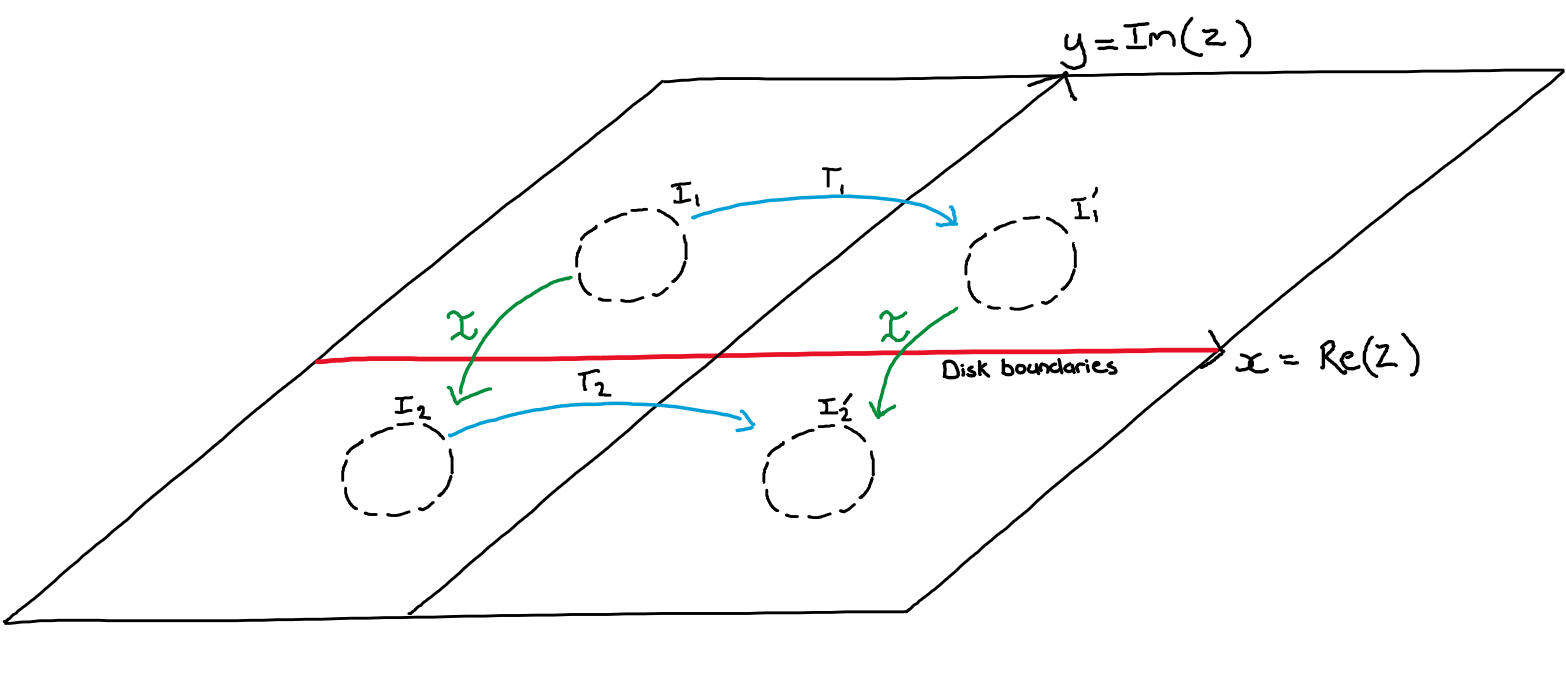
Figure 1: $\Sigma$ and its opposite orientation copy are related by the involution $I$ (shown in green), which is simply complex conjugation.

Thus, the Weil-Petersson measure for $\Sigma$ is given by

$$d\mu_{\mathrm{WP},\Sigma}=\frac{d^{2}k_{1}d^{2}\xi_{1}d^{2}\eta_{1}}{|k_{1}|^{4}|\eta_{1}-\xi_{1}|^{4}}|1-k_{1}|^{4},$$ (79)

whilst the integrand derived from the result for $\Sigma^{2}$ is simply restricted to the appropriate subset of moduli space. Thus, we obtain the result

$$W_{\Sigma}= \frac{1}{\sqrt{\Omega}}\int_{\mathrm{mod}(\Sigma)}\frac{d^{2}k_{1}d^{2}\xi_{1}d^{2}\eta_{1}}{|k_{1}|^{4}|\eta_{1}-\xi_{1}|^{4}}|1-k_{1}|^{4}(\frac{1}{2\pi}R_{\Sigma^{2},I}(J))^{-\frac{13}{2}}$$ (80)

$$\bigg{(}(\det\ \mathrm{Im}\ \tau)^{-13}\ \prod^{\prime}_{\alpha}\prod_{n=1}^{\infty}|1-k_{\alpha}^{n}|^{-48}\prod^{\prime}_{\alpha}|1-k_{\alpha}|^{-4}\bigg{)}^{\frac{1}{2}}\ e^{-I_{\mathrm{cl}}(X,g)}\ ,$$

where the term is brackets is calculated for the case where the relations in 78 hold.

3.3 Period Matrix Parametrisation

Alternatively, the method in BLAU1988285 used to calculate the partition function of the three-holed sphere can be immediately adapted to the disc-with-handle. Here one uses the period matrix to parametrise the moduli space. Up to a constant independent of the metric one has BLAU1988285

$$d\mu_{\mathrm{WP},\Sigma}\left({(\det(P_{1}^{\dagger}P_{1})_{g,\Sigma^{2}})^{\frac{1}{2}}}\left(\frac{\det^{\prime}(\Delta)_{g,\Sigma^{2}}}{\det\ \textrm{Im}\ \tau\int_{\Sigma^{2}}\sqrt{g}}\right)^{-13}\right)^{\frac{1}{2}}$$

$$= \underbrace{\prod_{1\geq i\geq j\geq 2}\{\frac{1}{2}(1+I^{*})d\ \mathrm{Im}\ \tau+\frac{1}{2}(1+I^{*})d\ \mathrm{Re}\ \tau\}_{ij}}_{\text{Weil-Petersson Measure}}\prod_{\alpha\ \textrm{even}}|\theta^{2}\{\alpha\}(0,\tau)|^{-1}$$ (81)

where the second product is of the ten even genus two theta functions. Note that the Weil-Petersson measure for $\Sigma$ is given in terms of the imaginary and real parts of the period matrix $\tau$ of the doubled surface $\Sigma^{2}$. The integration, however, is over the subset of the Teichmuller space of $\Sigma^{2}$ which corresponds to the Teichmuller space of $\Sigma$. To calculate the Weil-Petersson measure, we use the fact that

$$I^{*}\tau=-\Gamma^{T}\bar{\tau}\Gamma,\hskip 14.22636pt\Gamma=\begin{pmatrix}0&1\\ 1&0\end{pmatrix}.$$ (82)

Note that the Teichmuller space of the double torus is the Siegel upper half-space with the subspace of diagonal period matrices removed Rodrigues:1986us . Denoting $\tau$ as

$$\tau=\begin{pmatrix}a+ib&c+id\\ c+id&e+if\end{pmatrix},$$ (83)

we obtain

$$\prod_{1\geq i\geq j\geq 2}\{\frac{1}{2}(1+I^{*})d\ \mathrm{Im}\ \tau+\frac{1}{2}(1+I^{*})d\ \mathrm{Re}\ \tau\}_{ij}=\frac{1}{2}dx\wedge dy\wedge dz,$$ (84)

where we have made a change of variables

$$x=b+f,\ \ \ \ y=d,\ \ \ \ z=a-e.$$ (85)

We find now that

$$R_{\Sigma^{2},I}(J) =\frac{2}{bf-d^{2}}((b+d)^{2}+(d+f)^{2})$$ (86)

$$=\frac{4x^{2}+16y(x+y)}{x^{2}-(b-f)^{2}-4y^{2}}.$$

Compiling everything,

$$W_{\Sigma}\propto\frac{1}{\Omega^{\prime}}\int dxdydz\left(x^{2}+4y(x+y)\right)^{-\frac{13}{2}}\prod_{\alpha\ \textrm{even}}|\theta^{2}\{\alpha\}(0,\tau)|^{-1}\ e^{-I_{\mathrm{cl}}(X,g)}.$$ (87)

Note that we are integrating over all period matrices of the form

$$\tau=\begin{pmatrix}\frac{1}{2}(z+ix)&iy\\ iy&\frac{1}{2}(z+ix)\end{pmatrix}$$ (88)

subject to the condition that $\tau$ is in the Siegel upper half space with the subspace of diagonal period matrices removed Rodrigues:1986us . We integrate over Teichmuller space and then ‘divide out’ by the volume $\Omega^{\prime}$ of the mapping class group of the disc-with-handle, which is the 3-stranded braid group. As before, the classical action is a function of the moduli, however, we do not evaluate it in this thesis.

4 Conclusion

In this paper, we have reduced the infinite dimensional path integral for the partition functions of the string world-sheets ending on a fixed circular curve with annular topology and with the disc-with-handle topology to finite dimensional integrals over moduli parameters. For the annular topology, the partition function reduced to a one dimensional (divergent) integral over the inner radius of the annulus. To do this we calculated the determinant of the Laplacian operator on the annulus for the cases of Dirichlet-Dirichlet and Dirichlet-Neumann boundary conditions, which are factors that appear in the integrand.

For the case of the disc-with-handle, we pursued two different methods in computing the partition function. In both cases, we utilised the Schottky double of the surface, that is the surface obtained by gluing the disc-with-handle to itself. This eliminates the problem of having to deal with a boundary on the surface. We then used the fact that determinants on a Schottky double are the square of Laplacian determinants on the single copy of the surface, and that we can write the Weil-Petersson measure on the single-copy surface via the Weil-Petersson measure on the doubled surface. We obtained the final result twice, first using Schottky parameters of the moduli space, and then using the period matrix.

References

• (1) J.ย Maldacena, Wilson loops in large $\mathit{N}$ field theories, Phys. Rev. Lett. 80 (1998) 4859โ€“4862, [hep-th/9803002].
• (2) N.ย Drukker, D.ย J. Gross, and H.ย Ooguri, Wilson loops and minimal surfaces, Phys. Rev. D 60 (1999) 125006, [hep-th/9904191].
• (3) N.ย Drukker, D.ย J. Gross, and A.ย A. Tseytlin, Green-Schwarz string in AdS${}_{5}\times{\rm S}^{5}$: Semiclassical partition function, JHEP 04 (2000) 021, [hep-th/0001204].
• (4) R.ย Kallosh and A.ย A. Tseytlin, Simplifying superstring action on AdS${}_{5}\times{\rm S}^{5}$, JHEP 10 (1998) 016, [hep-th/9808088].
• (5) S.ย Forste, D.ย Ghoshal, and S.ย Theisen, Stringy corrections to the Wilson loop in N=4 superYang-Mills theory, JHEP 08 (1999) 013, [hep-th/9903042].
• (6) D.ย Medina-Rincon, A.ย A. Tseytlin, and K.ย Zarembo, Precision matching of circular Wilson loops and strings in AdS5 ร— S5, JHEP 05 (2018) 199, [arXiv:1804.08925].
• (7) S.ย Giombi and A.ย A. Tseytlin, Strong coupling expansion of circular Wilson loops and string theories in AdS${}_{5}\times{\rm S}^{5}$ and AdS${}_{4}\times{\rm CP}^{3}$, JHEP 10 (2020) 130, [arXiv:2007.08512].
• (8) N.ย Drukker and D.ย J. Gross, An Exact prediction of N=4 SUSYM theory for string theory, J. Math. Phys. 42 (2001) 2896โ€“2914, [hep-th/0010274].
• (9) S.ย Giombi and B.ย Offertaler, Wilson loops in $\mathcal{N}=4$ $SO(N)$ SYM and D-Branes in $AdS_{5}\times\mathbb{RP}^{5}$, arXiv:2006.10852.
• (10) C.ย Graham, K.ย Kirsten, P.ย Morales-Almazan, and B.ย Q. Streit, Functional determinants for Laplacians on annuli and elliptical regions, J. Math. Phys. 59 (2018), no.ย 1 013508.
• (11) S.ย K. Blau, M.ย Clements, S.ย D. Pietra, S.ย Carlip, and V.ย D. Pietra, The string amplitude on surfaces with boundaries and crosscaps, Nucl. Phys. B 301 (1988) 285โ€“303.
• (12) O.ย Alvarez, Theory of Strings with Boundaries: Fluctuations, Topology, and Quantum Geometry, Nucl. Phys. B 216 (1983) 125โ€“184.
• (13) J.ย P. Rodrigues, One Loop Amplitudes for the Bosonic Open String: A First Quantized Approach, Phys. Lett. B 178 (1986) 350โ€“356.
• (14) M.ย Nakahara, Geometry, topology and physics. Taylor & Francis Group, 2003.
• (15) K.ย Kirsten, Spectral functions in mathematics and physics, AIP Conf. Proc. 484 (1999), no.ย 1 106โ€“146, [hep-th/0005133].
• (16) L.ย Brink and D.ย B. Fairlie, Pomeron singularities in the fermion meson dual model, Nucl. Phys. B 74 (1974) 321โ€“342.
• (17) A.ย A. Tseytlin, Renormalization group and string loops, Int. J. Mod. Phys. A 5 (1990) 589โ€“658.
• (18) P.ย Diย Vecchia, M.ย Frau, A.ย Lerda, and S.ย Sciuto, A Simple Expression for the Multiloop Amplitude in the Bosonic String, Phys. Lett. B 199 (1987) 49โ€“56.