Learning Invariant Representations with Missing Data

Abstract

Spurious correlations allow flexible models to predict well during training but poorly on related test distributions. Recent work has shown that models that satisfy particular independencies involving correlation-inducing nuisance variables have guarantees on their test performance. Enforcing such independencies requires nuisances to be observed during training. However, nuisances, such as demographics or image background labels, are often missing. Enforcing independence on just the observed data does not imply independence on the entire population. Here we derive mmd estimators used for invariance objectives under missing nuisances. On simulations and clinical data, optimizing through these estimates achieves test performance similar to using estimators that make use of the full data.

1 Introduction

Spurious correlations allow models that predict well on training data to have worse than chance performance on related distributions at test time (Geirhos et al., 2020; Puli et al., 2022; Veitch et al., 2021; Makar et al., 2021; Gulrajani and Lopez-Paz, 2020; Sagawa et al., 2020). For example, diabetes is associated with high body mass index (bmi) in the United States. However, in India and Taiwan, diabetes also frequently co-occurs with low and average bmi (WHO, 2004). Due to their shifting relationship with the label, nuisance variables (e.g., bmi) can cause models to exploit non-causal correlations in training data, leading models to generalize poorly.

Invariant prediction methods are designed to improve performance on a range of test distributions when training data exhibits spurious correlations (Peters et al., 2016; Arjovsky et al., 2019). We focus on methods that enforce independencies between the model and nuisance given some assumed causal structure (Makar et al., 2021; Veitch et al., 2021; Puli et al., 2022). These methods require the nuisance to be specified explicitly and observed. Nuisances must be observed for all samples because independence constraints are enforced via metrics such as Maximum Mean Discrepancy (mmd), which require samples from the fully-observed data. However, in large health datasets, nuisances are often missing. For example, not all people who report diabetes status report other correlated conditions (e.g., hypertension, depression) or demographics (e.g., gender). To improve generalization on a range of test distributions, it is necessary to handle missingness appropriately.

We propose mmd estimators for measuring nuisance-model dependence under nuisance missingness. First, we show that enforcing independence on only the nuisance-observed data does not imply independence on the full data distribution, and vice versa. Next, we derive three estimators, including one that is doubly-robust: it is consistent when either the nuisance or its missingness can be consistently modeled given covariates (Bang and Robins, 2005). Using simulations, a semi-simulation based on textured mnist and clinical data from mimic, we show that the estimators perform close to ground-truth estimation with no missingness and that they improve test accuracy relative to computing the original objective only on samples with nuisances observed.

2 Notation and background

Notation.

Let $X$ denote features. Let $Y$ be a label such as disease status. Let $Z$ denote the nuisance, e.g., another disease correlated with $Y$, demographics, or image backgrounds. Denote the nuisance missingness indicator as $\Delta$. Instead of $(X,Y,Z)$, we observe $(X,Y,\Delta,\tilde{Z}=\Delta Z)$, where $\tilde{Z}=Z$ when $\Delta=1$ and $Z$ is unobserved otherwise. We write functions as $f_{X}=f(X)$. Let $h_{X}$ denote a model to predict $Y$. When conditioning on events involving both $X,Y$ we use $W=(X,Y)$ and $w=(x,y)$ to lighten notation so that $\mathop{\mathbb{E}}[\Delta|X=x,Y=y]=\mathop{\mathbb{E}}[\Delta|W=w]$ and $f(X,Y)=f_{XY}=f_{W}$. Let $\mathcal{B}(p)$ denote $\text{Bernoulli}(p)$.

Modeling under spurious correlations.

Nuisance-based prediction arises in training data when $Z$ is predictive of $Y$ and associated with $X$, causing models to use information about $Z$ in $X$ to predict $Y$. This may not be a problem in all scenarios, but it is when the test distribution is expected to have a different $(Y,Z)$ relationship from the training distribution, as this may imply $P_{train}(Y~{}|~{}X)\neq P_{test}(Y|X)$ and a model built on training data may not perform well on test data. Most approaches to this problem start off by narrowing down the set of possible test distributions and their relationship to the training distribution. In this work, we focus on a family studied in Makar et al. (2021); Veitch et al. (2021); Puli et al. (2022). The distributions are indexed by $D$ and vary only in the factor $P(Z~{}|~{}Y)$:

$$\mathcal{F}=\{P_{D}(X,Y,Z)=P(Y)P_{D}(Z|Y)P(X|Y,Z)\}_{D}.$$ (1)

When $P_{test}(Z|Y)\neq P_{train}(Z|Y)$, in general $P_{train}(Y~{}|~{}X)\neq P_{test}(Y|X)$ and a model built on $P_{train}$ can generalize poorly. For example consider, for $a\in\mathbb{R}$,

$$Y\sim\mathcal{B}(0.5),\quad\mu_{Z}=a(2Y-1),\quad Z\sim\mathcal{N}(\mu_{Z},1).$$

When $P_{train}$ uses $a=0.5$ and $P_{test}$ uses $a=-0.9$, Puli et al. (2022) show an example of an $X|Y,Z$ distribution where an ERM model that predicts $Y$ from $X$ with $80\%$ training accuracy only achieves $40\%$ on the test set, due to the changing relationship between $Y,Z$, even when $Z$ is not an input feature to the model.

When it is possible to anticipate and observe nuisances during training, enforcing certain independence constraints (Makar et al., 2021; Veitch et al., 2021; Puli et al., 2022) helps guarantee performance regardless of the nuisance-label relationship. For example, for this choice of $\mathcal{F}$ and model $h$, maximum likelihood estimation for $Y|h_{X}$ while enforcing the constraint $h_{X}\rotatebox[origin={c}]{90.0}{$\models$}Z~{}|~{}Y$ implies equal performance on all $P_{D}\in\mathcal{F}$, and better than chance performance (Appendix A).

Measuring Dependence.

To enforce independencies it is necessary to measure dependence and to minimize this measure. One way to measure dependence is to measure distance between a joint distribution and the product of its marginals. The general Integral Probability Metrics (ipms) class defines a metric on distributions. A special case, the kernel-based mmd (Gretton et al., 2012), has a closed form. Let $X_{1}\sim P,X_{2}\sim Q$. Let $X_{j}^{\prime}$ be an independent sample identically distributed as $X_{j}$. For kernel $k$,

$$\lx@glossaries@gls@link{acronym}{mmd}{\leavevmode\textsc{mmd}}_{k}(P,Q)=\mathop{\mathbb{E}}[k(X_{1},X_{1}^{\prime})]+\mathop{\mathbb{E}}[k(X_{2},X_{2}^{\prime})]-2\mathop{\mathbb{E}}[k(X_{1},X_{2})]\,.$$ (2)

The mmd is $0$ if and only if $P=_{d}Q$ under certain mild conditions on $P,Q$ and the kernel $k$ (Gretton et al., 2012). Computing the mmd on a joint distribution $P$ of two variables and the product of its marginals $Q$ is a measure dependence, which also coincidences with the Hilbert-Schmidt Independence Criterion (hsic) (Gretton et al., 2005; Szabó and Sriperumbudur, 2017).

Assumptions and scope.

The estimators in this work require ignorability: $Z\rotatebox[origin={c}]{90.0}{$\models$}\Delta|W$ (Hernan and Robins, 2021). This holds, e.g., in graphs such as Figure 1. We also require positivity $0<\epsilon\leq P(\Delta=1|W)$ to observe $Z$ appropriately. While we focus on the graph in Figure 1 with binary $Z$, the presented method can extend to continuous $Z$ (Appendix H), to other data generating processes, and to other invariance objectives. The method applies when the data distributions satisfy ignorability, positivity, and any assumptions made by the underlying invariance method.

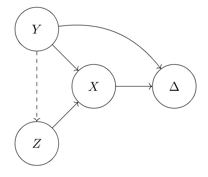
Figure 1: Generative process we consider in this work. The $Y\rightarrow Z$ edge is dashed to emphasize that the $Z|Y$ may change at test time. $\Delta$ determines missingness of $Z$ and satisfies $Z\rotatebox[origin={c}]{90.0}{$\models$}\Delta|(X,Y)$.

Estimation under missingness.

The problem that this work tackles is enforcing conditional independencies such as $h_{X}\rotatebox[origin={c}]{90.0}{$\models$}Z|Y$ to improve generalization in families like $\mathcal{F}$ in Equation 1 even when $Z$ is subject to missingness. Methodology from causal inference solves a related problem: estimating $\mathop{\mathbb{E}}[Z]$ when $Z$ is subject to missingness. In this work, we extend this methodology from estimates of $\mathop{\mathbb{E}}[Z]$ to estimates of objectives that enforce independencies involving $Z$. Here we review estimation of $\mathop{\mathbb{E}}[Z]$ under missingness. The following assumes ignorability and positivity. Two parts of the data-generating distribution can help. Letting $W=(X,Y)$, define:

$$G_{W} \triangleq\mathbb{E}[\Delta~{}|~{}X,Y]\quad\quad\text{(missingness process)}$$

$$m_{W} \triangleq\mathbb{E}[Z~{}|~{}X,Y]\quad\quad\text{(conditional expectation)}$$

We review estimators of $\mathop{\mathbb{E}}[Z]$ that use $G_{W}$ (Horvitz and Thompson, 1952; Binder, 1983; Robins et al., 1994) or $m_{W}$ (Rubin, 1976; Schafer, 1997) in Appendix E. The doubly-robust (dr) estimator (Robins and Rotnitzky, 2001; Bang and Robins, 2005; Kang and Schafer, 2007) combines both by noting the following equality:

$$\mathop{\mathbb{E}}[Z]=\mathop{\mathbb{E}}\Big{[}\frac{\Delta\tilde{Z}}{G_{W}}-\frac{\Delta-G_{W}}{G_{W}}m_{W}\Big{]}\,.$$ (3)

Crucially, the right side of Equation 3 does not requires samples of $Z$ when $\Delta=0$. When $G_{W}$ or $m_{W}$ are replaced with estimates $\hat{G}_{W},\hat{m}_{W}$, the equality still holds provided that for all $w$, either $\hat{G}_{w}=G_{w}$ or $\hat{m}_{w}=m_{w}$ (Appendix F). Moreover, Monte Carlo estimates of the right side of Equation 3 are consistent for $\mathop{\mathbb{E}}[Z]$ when either $\hat{G}_{W}$ consistently estimates $G_{W}$ or $\hat{m}_{W}$ consistently estimates $m_{W}$ (Robins and Rotnitzky, 2001). This is useful because in practice neither of $G_{W}$ nor $m_{W}$ are known and both must be estimated.

3 Invariant representations with missing data

For the graph in Figure 1 and binary $Z$, Veitch et al. (2021) enforce $h_{X}\rotatebox[origin={c}]{90.0}{$\models$}Z|Y$ for the predictive model $h$ by maximizing likelihood while minimizing the mmd:

$$\max_{h}\,\quad\log p(y|h_{X})-\lambda\cdot\sum_{y\in\{0,1\}}\lx@glossaries@gls@link{acronym}{mmd}{\leavevmode\textsc{mmd}}_{k}\left(p(h_{X}|Z=1,Y=y)\,,\,p(h_{X}|Z=0,Y=y)\right)\,,$$ (4)

for $\lambda\geq 0$. The first term is the usual maximum-likelihood objective for predicting $y$ with model $h_{X}$. The second term, because $Z$ is binary, enforces $h_{X}\rotatebox[origin={c}]{90.0}{$\models$}Z|Y$ when minimized. First, we motivate the independence constraint for the choice of assumed family $\mathcal{F}$ in Equation 1. We then demonstrate what can go wrong when enforcing this mmd penalty only on samples where $Z$ is observed. We then derive estimators of the full-data mmd under missingness.

3.1 Conditional Independence implies equal performance on the anti-causal family

There are at least two distinct usages of the word invariance in the literature. One refers to independence (e.g. of a model to a nuisance or environment variable). The other refers to invariant risk, i.e., the risk is the same for all test distributions in some family (Arjovsky et al., 2019; Krueger et al., 2021). In some families and for some independence constraints, these can coincide.

Proposition 1

Suppose model $h_{X}$ satisfies $h_{X}\rotatebox[origin={c}]{90.0}{$\models$}Z|Y$ on any $P_{D}\in\mathcal{F}$. Then for all $P_{D^{\prime}}\in\mathcal{F}$, $\mathop{\mathbb{E}}_{P_{D}}[\log p_{D}(Y|h_{X})]=\mathop{\mathbb{E}}_{P_{D^{\prime}}}[\log p_{D}(Y|h_{X})]$.

This has been shown in Veitch et al. (2021); Puli et al. (2022) but we provide a self-contained proof in Appendix A. This result means that estimates of held-out performance from the training data (one member of $\mathcal{F}$) will represent test performance on other member of $\mathcal{F}$ under $h_{X}\rotatebox[origin={c}]{90.0}{$\models$}Z|Y$.

3.2 Failures of restricting to observed data

Under missingness, we observe $(X,Y,\Delta,\tilde{Z})$ instead of $(X,Y,Z)$, where $\Delta=1$ means $\tilde{Z}=Z$ and $Z$ is unobserved when $\Delta=0$. When $Z$ is subject to missingness, we cannot directly compute empirical estimates of the mmd. What happens when we compute the mmd only on samples with $Z$ observed? Let us refer to this as the observed-only mmd. Restricting computation to data with non-missing $Z$ enforces $h_{X}\rotatebox[origin={c}]{90.0}{$\models$}Z|Y=y,\Delta=1$ instead of $h_{X}\rotatebox[origin={c}]{90.0}{$\models$}Z|Y=y$. We show that these conditions do not imply each other in general.

Proposition 2

There exist distributions on $(X,Y,\Delta,Z)$ such that

$$\exists h_{X}^{\star}\quad\text{s.t.}\quad h_{X}^{\star}\rotatebox[origin={c}]{90.0}{$\models$}Z|Y=y,\quad\text{but}\quad h_{X}^{\star}\rotatebox[origin={c}]{90.0}{$\not\models$}Z|Y=y,\Delta=1$$

and there exist distributions on $(X,Y,\Delta,Z)$ such that

$$\exists h_{X}^{\star}\quad\text{s.t.}\quad h_{X}^{\star}\rotatebox[origin={c}]{90.0}{$\models$}Z|Y=y,\Delta=1\quad\text{but}\quad h_{X}^{\star}\rotatebox[origin={c}]{90.0}{$\not\models$}Z|Y=y$$

The proof is in Appendix D. This existence implies:

1. Optimizing the observed-only mmd can discard a solution to the full-data mmd

2. Using the observed-only mmd may lead one to believe a model is invariant when it is not.

To keep generalization guarantees one must enforce independence on the full data distribution.

3.3 Mmd estimation under missingness

We present estimators of the full-data unconditional mmd under missing $Z$ , which enforces $h_{X}\rotatebox[origin={c}]{90.0}{$\models$}Z$ (unconditional on $Y$). Everything that follows can be conditioned on $Y=y$ to enforce $h_{X}\rotatebox[origin={c}]{90.0}{$\models$}Z|Y=y$ simply by restricting samples used to estimate the expectations to those with $Y=y$. For a kernel $k$ let $k_{XX^{\prime}}\triangleq k(h_{X},h_{X^{\prime}})$. The mmd can be written as:

$$\lx@glossaries@gls@link{acronym}{mmd}{\leavevmode\textsc{mmd}}_{k}\big{(}p(h_{X}|Z=1),p(h_{X}|Z=0)\big{)}=\mathop{\mathbb{E}}_{\begin{subarray}{c}X|Z=1\\ X^{\prime}|Z^{\prime}=1\end{subarray}}k_{XX^{\prime}}+\mathop{\mathbb{E}}_{\begin{subarray}{c}X|Z=0\\ X^{\prime}|Z^{\prime}=0\end{subarray}}k_{XX^{\prime}}-2\mathop{\mathbb{E}}_{\begin{subarray}{c}X|Z=1\\ X^{\prime}|Z^{\prime}=0\end{subarray}}k_{XX^{\prime}}\,.$$ (5)

Estimation is challenging due to missingness in the conditioning set. For $b,b^{\prime}\in\{0,1\}$, let $N(b,b^{\prime})\triangleq P(Z=b)P(Z^{\prime}=b^{\prime})$ and let $Z_{1}\triangleq Z$ and $Z_{0}\triangleq 1-Z$. For any of the expectations, the dependence on $Z$ can be re-written with indicators in a joint expectation:

$$\mathop{\mathbb{E}}_{\begin{subarray}{c}X|Z=b\\ X^{\prime}|Z^{\prime}=b^{\prime}\end{subarray}}k_{XX^{\prime}}=\frac{1}{N(b,b^{\prime})}\mathop{\mathbb{E}}\Big{[}k_{XX^{\prime}}\cdot Z_{b}\cdot Z^{\prime}_{b^{\prime}}\Big{]}\,,$$ (6)

Under no missingness, each expectation could be estimated with Monte Carlo. We now develop three estimators for these expectations. We propose simple $G_{W}$-based and $m_{W}$-based estimators in Equations 7 and 8 and then a doubly-robust estimator that combines them in Equation 9.

Proposition 3

($G_{W}$-based re-weighted estimator) Assume positivity, ignorability, and, $\forall w$, $G_{w}=\mathop{\mathbb{E}}[\Delta|W=w]$. Then,

$$\mathop{\mathbb{E}}_{\begin{subarray}{c}X|Z=b\\ X^{\prime}|Z^{\prime}=b^{\prime}\end{subarray}}\Big{[}k_{XX^{\prime}}\Big{]} =\frac{1}{N(b,b^{\prime})}\mathop{\mathbb{E}}\Big{[}\frac{\Delta\Delta^{\prime}\tilde{Z}_{b}\tilde{Z^{\prime}}_{b^{\prime}}}{G_{WW^{\prime}}}k_{XX^{\prime}}\Big{]}.$$ (7)

Proposition 4

($m_{W}$-based regression estimator) Assume ignorability, and, $\forall w$, $m_{w}=\mathop{\mathbb{E}}[Z|W=w]$. Then,

$$\mathop{\mathbb{E}}_{\begin{subarray}{c}X|Z=b\\ X^{\prime}|Z^{\prime}=b^{\prime}\end{subarray}}\Big{[}k_{XX^{\prime}}\Big{]} =\frac{1}{N(b,b^{\prime})}\mathop{\mathbb{E}}\Big{[}m_{Wb}\cdot m_{W^{\prime}b^{\prime}}\cdot k_{XX^{\prime}}\Big{]}.$$ (8)

Let $m_{W1}\triangleq m_{W},\phantom{.}m_{W0}\triangleq 1-m_{W}$, and $G_{WW^{\prime}}\triangleq G_{W}G_{W^{\prime}}$.

Proposition 5

(dr estimator). Assume positivity, ignorability, and $\forall w$, either $G_{w}=\mathop{\mathbb{E}}[\Delta|W=w]$ or $m_{w}=\mathop{\mathbb{E}}[Z|W=w]$. Then,

$$\mathop{\mathbb{E}}_{\begin{subarray}{c}X|Z=b\\ X^{\prime}|Z^{\prime}=b^{\prime}\end{subarray}}\Big{[}k_{XX^{\prime}}\Big{]} =\frac{1}{N(b,b^{\prime})}\mathop{\mathbb{E}}\Big{[}\Big{(}\frac{\Delta\Delta^{\prime}\tilde{Z}_{b}\tilde{Z^{\prime}}_{b^{\prime}}}{G_{WW^{\prime}}}-\frac{\Delta\Delta^{\prime}-G_{WW^{\prime}}}{G_{WW^{\prime}}}\cdot m_{Wb}\cdot m_{W^{\prime}b^{\prime}}\Big{)}k_{XX^{\prime}}\Big{]}\,.$$ (9)

The proof is in Appendix G. We can use any of Equations 7, 8 and 9 to estimate the terms in eq. 5. Each of Equations 7, 8 and 9 is a ratio of two expectations: the normalization constant $N(b,b^{\prime})$ depends on $\mathop{\mathbb{E}}[Z]$ and must itself be estimated under missingness (e.g., with Equation 3). The ratio of consistent estimates of these quantities is consistent by Weak Law of Large Numbers and Slutsky’s theorem. We discuss estimation in practice, trade-offs among the three estimators, and variance in Appendix B. We review recent related work in Section 5.

4 Experiments

We compare accuracy and mmd minimization using different estimators: none (mle only, no mmd), full (mle and mmd using data with $Z$ fully-observed, which is what could be used as an objective under no missingness), obs (mle and observed-only mmd), dr (mle and dr estimator, called dr + when using true $G_{W}$), ip (mle and re-weighted estimator, called ip + when using true $G_{W}$), and reg (mle and regression estimator).

We first compare these algorithms in a simulation study. We then use textured mnist to show the utility of the proposed estimators on high-dimensional data. In quantitative tables, we show mean $\pm$ standard deviation over three seeds. We then predict hospital length of stay in the mimic dataset, and compare performance when demographic nuisances are subject to missingness. For the $Y|X$ predictive loss, we use negative Bernoulli log likelihood with logit equal to model output $h_{X}$.

Comparing mmds.

In all tables, the training set mmd to evaluate each method is computed using the ground-truth full-data mmd estimation method (see eq. 6) to show the actual value of mmd achieved, regardless of optimization method. This is also what the full method directly optimizes. True $Z$’s are available in both simulated and real data as missingness is simulated. However, each model trains and validates the $\log p(Y|X)+\lx@glossaries@gls@link{acronym}{mmd}{\leavevmode\textsc{mmd}}$ loss using its own estimation method for mmd.

4.1 Experiment 1: Simulation.

We set up strong $(Y,Z)$ correlation. With $\overline{Y}=1-Y$, the training and validation sets are drawn:

$$\begin{split}Y\sim\mathcal{B}(0.5),\quad Z\sim\mathcal{B}(.9Y+.1\overline{Y}),\quad X\sim[\mathcal{N}(Y-Z,\sigma_{X}^{2}),\mathcal{N}(Y+Z,\sigma_{X}^{2})]\,.\end{split}$$ (10)

The test set has the opposite relationship $Z\sim\mathcal{B}(.1Y+.9\overline{Y})$. Here $h_{X}^{\star}=(X_{1}+X_{2})/2$ predicts $Y$ with smallest MSE among representations satisfying independence. We construct $\Delta$ to show the failure of computing mmd on the observed-only subset. For this, we use $\hat{Z}\triangleq-(X_{1}-X_{2})/2$, which is correlated with $Z$. We draw $\Delta$ conditional on $h_{X}^{\star}$ and $\hat{Z}$ (both are functions of $X$):

$$Q=\mathbbm{1}\left[h_{X}^{\star}>0.6\right]\cdot\mathbbm{1}\left[\hat{Z}<0.6\right],\quad\Delta\sim\mathcal{B}(Q+0.2\overline{Q})\,.$$

This example construction leads to $h_{X}^{\star}\rotatebox[origin={c}]{90.0}{$\models$}Z|Y$ but $h_{X}^{\star}\rotatebox[origin={c}]{90.0}{$\not\models$}Z|Y,\Delta=1$. For $h,G_{W}$ and $m_{W}$ we use small feed-forward neural networks. See the repository for more details.

Results.

In Table 1, the dr estimators achieve indistinguishable performance to the full-data mmd, both in mmd and accuracy, and better than none and obs. We include more results in Appendix C.

Table 1: Simulation. $\lambda=1$. None has highest mmd and lowest test accuracy. Obs improves over this. The dr and reg methods are able to bring the mmd close to $0.0$ and attain best test accuracy.

	none	obs	full	dr	dr +	reg
tr mmd	$0.21\pm 0.04$	$0.05\pm 0.04$	$0.00\pm 0.01$	$0.00\pm 0.01$	$0.00\pm 0.01$	$0.01\pm 0.00$
tr acc	$0.89\pm 0.00$	$0.87\pm 0.00$	$0.86\pm 0.01$	$0.85\pm 0.01$	$0.84\pm 0.02$	$0.86\pm 0.00$
te acc	$0.67\pm 0.02$	$0.77\pm 0.02$	$0.80\pm 0.01$	$0.81\pm 0.02$	$0.81\pm 0.01$	$0.79\pm 0.02$

4.2 Experiment 2: Textured mnist.

Following Goodfellow et al. (2013), we correlate mnist digits $0$ and $1$ with two textures from the Brodatz dataset (Figure 2). This is an example of invariance to image backgrounds when not all background labels are available. We follow a similar setup to colored mnist (Arjovsky et al., 2019): because $Y|X$ is essentially deterministic, even strong spurious correlations may be ignored by a model on mnist. To push $Y|X$ closer to what may be expected in noisier real data, we flip the label with 25% chance. Letting $X$ only predict $Y$ with $75\%$ chance means the model will use texture instead. The missingness is based on the average pixel intensity of $X$ and its class. Let $\mu_{X}$ be the mean pixel value of a 28x28 mnist image. We set

$$Q=\mathbbm{1}\left[Y=1\right]\cdot\mathbbm{1}\left[\mu_{X}<0.3\right],\quad\Delta\sim\mathcal{B}(Q+.2\overline{Q}).$$

The choice of $Q$ is correlated with $Z$ through whether the image is light or dark grey. Similar to proposition 2 and experiment 1, this means subsetting on $\Delta=1$ does not imply independence on the full population and may throw away solutions that do.

Figure 2: Textured mnist with digits 0,1 on two textures from the Brodatz dataset.

For $h,G_{W}$ and $m_{W}$ we use small convolutional networks. We include more details in the repository.

Results.

In Table 2, none and obs perform poorly on test. In contrast, the dr estimators — including the one with a learned $G_{W},m_{W}$ — achieve close to full’s performance.

Table 2: mnist $\lambda=1$. dr and reg estimators achieve close to full performance as measured by full mmd $=0$ and high test accuracy. None and obs perform poorly on test. Obs is notably high variance.

	none	obs	full	dr	dr +	reg
tr mmd	$2.05\pm 0.18$	$0.02\pm 0.04$	$0.00\pm 0.01$	$0.00\pm 0.01$	$0.00\pm 0.01$	$0.00\pm 0.01$
tr acc	$0.90\pm 0.01$	$0.74\pm 0.03$	$0.76\pm 0.01$	$0.77\pm 0.0$	$0.76\pm 0.01$	$0.76\pm 0.01$
te acc	$0.13\pm 0.01$	$0.63\pm 0.17$	$0.74\pm 0.01$	$0.72\pm 0.04$	$0.73\pm 0.01$	$0.73\pm 0.01$

4.3 Experiment 3: Predicting length of stay in the icu

We predict length of stay in the intensive care unit (icu) in mimic (Johnson et al., 2016) using demographics and first day labs/vitals among patients that stay at least one day. The prediction task is whether the stay is more than $2.5$ days. To demonstrate that spurious correlations cause issues at deployment, we choose $Z=1$ to indicate the patient is recorded as white. While race may be correlated with health outcomes (e.g., due to unobserved socioeconomic factors (Obermeyer et al., 2019)), it may not always be appropriate for a model to use this information (Chen et al., 2018). The test set represents a new population with different outcome-demographic structure: we split the data so that the training/validation set has mostly samples with $Y\neq Z$ while the test set has mostly samples with $Y=Z$. We set non-male patients to have $Z$ observed with probability $0.2$. We include more details in the repository.

Table 3: mimic $\lambda=1$. reg estimator matches full’s performance and improves upon obs while dr does not, due to high objective variance during training (not shown in table).

	none	obs	full	dr	reg
tr mmd	$0.017\pm 0.02$	$0.002\pm 0.01$	$0.00\pm 0.00$	$0.009\pm 0.01$	$0.00\pm 0.00$
tr acc	$0.71\pm 0.02$	$0.68\pm 0.01$	$0.70\pm 0.01$	$0.70\pm 0.01$	$0.71\pm 0.00$
te acc	$0.64\pm 0.00$	$0.64\pm 0.00$	$0.66\pm 0.00$	$0.62\pm 0.00$	$0.66\pm 0.01$

Results.

In this real data setting with strong $(Y,Z)$ correlation, the full-data mmd estimator reported in the table for all methods may have high variance. We focus on the attained accuracies. The reg estimator matches the ground-truth full estimator and performs better than obs and dr. This is not unexpected, since it is possible for the reg estimator to be lower variance than dr when the true $G_{W}$ is small or $G_{W}$ is not modeled well (Davidian, 2005), especially under strong $(Y,Z)$ correlation (Appendix B).

5 Related work

We focus on recent work in fairness and invariant prediction on missing group/environment labels. Motivated by fairness, Wang et al. (2020) study a related problem of optimizing invariance-inducing objectives when the protected group label (analogous to our nuisance variables) is noisy. Given bounds on the level of label noise, this work proposes optimizing an objective based on the distributionally robust optimization framework (Namkoong and Duchi, 2016). Additionally, if given a small amount of true labels the authors suggest fitting a model to de-noise the noisy group labels and re-weight examples in the objective, which is similar in spirit to our work. In our approach, however, we exploit structural assumptions about the missingness process to build a doubly-robust estimator of the mmd penalty used during optimization.

Lahoti et al. (2020) optimize worst-case-over-groups performance without known group labels. They rely on the assumption that groups are computationally-identifiable (i.e. that there exists some function on the data that labels their protected group membership) (Hébert-Johnson et al., 2018) and use a model to identify groups on which performance is worst. They pose an adversarial optimization between the group-labeling model — which searches for groups with poor performance — and the primary predictive model. Inspired by this work, Creager et al. (2021) find worst-case group assignments based on an empirical risk minimization (erm) model that maximizes invariance penalties and Ahmed et al. (2020) illustrate that this objective performs well on a wide range of benchmarks. Relatedly, Liu et al. (2021) run usual erm training and then a second iteration of erm that upweights the loss for datapoints on which the model performs badly. This identifies groups with bad model performance without explicit group labels. In both of these works, the groups could be seen either as a nuisance variable or as a confounder that correlates the label and some nuisance variable. However, in our setting (and in that of Makar et al. (2021); Veitch et al. (2021); Puli et al. (2022)), in exchange for being willing to make assumptions on the test distribution family, we do not need to observe samples with poor model performance at training time (and may not see any) to prevent sudden decreases in performance on held-out data at test time.

6 Conclusion

We present estimators for the mmd that extend recent invariant prediction methods to missing data. Unlike prior estimators that only leverage data with nuisances observed, or consider worst-case estimation, the presented estimators of the full data objective are consistent when either auxiliary model can be learned. As we show in proposition 2, estimation of the full data objective is necessary to preserve the theoretical properties of invariant prediction methods. In the experiments, the dr and reg estimators are able to match full-data mmd performance and improve test accuracy relative to the obs estimator. In practice, we recommend exploring the two simpler proposed estimators (reg and ip) in addition to the dr estimator and selecting the model based on the validation metric.

Moving forward, one limitation is that the full-data estimator — used as ground-truth mmd evaluation for the experiments — may itself have high variance on small datasets with strong nuisance-label correlation. Variance reduction is an important avenue both for optimizing and evaluating with the mmd using smaller batch sizes (in our experiments, batch sizes $1500$ for mnist and $4000$ for mimic are large). Beyond variance reduction, it is a promising direction to apply the methodology in this work to the mutual information objective in Puli et al. (2022), which sidesteps the choice of kernel and may be better suited for continuous and high dimensional nuisances.

The authors thank Scotty Fleming, Joe Futoma, Leon Gatys, Sean Jewell, Tayor Killian, and Guillermo Sapiro for feedback and discussions. This work was in part supported by NIH/NHLBI Award R01HL148248, NSF Award 1922658 NRT-HDR: FUTURE Foundations, Translation, and Responsibility for Data Science, and NSF Award 1815633 SHF.

Appendix A Invariant predictor

Here, we show that $h_{X}\rotatebox[origin={c}]{90.0}{$\models$}Z|Y=y$ for all $y$ implies invariant risk in $\mathcal{F}$. The proof uses the following insights

• Satisfying independence $h_{X}\rotatebox[origin={c}]{90.0}{$\models$}Z~{}|~{}Y$ means $P_{train}(h_{X}|Y,Z)=P_{train}(h_{X}|Y)$.

• The assumptions on $\mathcal{F}$ mean $P_{train}(h_{X}|Y,Z)=P(h_{X}|Y,Z)$ in any member of the family.

• Combined this means $P_{train}(h_{X}|Y,Z)=P_{D}(h_{X}|Y)$ for any $P_{D}\in\mathcal{F}$ when the model $P_{train}(Y|h_{X})$ satisfies $h_{X}\rotatebox[origin={c}]{90.0}{$\models$}Z|Y$.

Proposition

Suppose model $h_{X}$ satisfies $h_{X}\rotatebox[origin={c}]{90.0}{$\models$}Z|Y$ on any $P_{D}\in\mathcal{F}$. Then for all $P_{D^{\prime}}\in\mathcal{F}$, $\mathop{\mathbb{E}}_{P_{D}}[\log p_{D}(Y|h_{X})]=\mathop{\mathbb{E}}_{P_{D^{\prime}}}[\log p_{D}(Y|h_{X})]$.

Proof A.1.

Consider test set performance $\mathop{\mathbb{E}}_{P_{test}(Y,X)}[\log P_{train}(Y|h_{X})]$. By the assumption on the family, by Bayes, and by satisfying the independence constraint:

$$\mathop{\mathbb{E}}_{P_{test}(Y,X)}[\log P_{train}(Y|h_{X})] =\mathop{\mathbb{E}}_{P_{test}(Y,X)}\Big{[}\log\frac{P_{train}(h_{X}|Y)P(Y)}{P_{train}(h_{X})}\Big{]}$$

$$=\mathop{\mathbb{E}}_{P_{test}(Y,X,Z)}\Big{[}\log\frac{P_{train}(h_{X}|Y,Z)P(Y)}{\mathop{\mathbb{E}}_{P(Y)}\Big{[}P_{train}(h_{X}|Y,Z)\Big{]}}\Big{]}$$

$$=\mathop{\mathbb{E}}_{P_{test}(Y,h_{X},Z)}\Big{[}\log\frac{P_{train}(h_{X}|Y,Z)P(Y)}{\mathop{\mathbb{E}}_{P(Y)}\Big{[}P_{train}(h_{X}|Y,Z)\Big{]}}\Big{]}$$

$$=\mathop{\mathbb{E}}_{P_{test}(Y,h_{X},Z)}\Big{[}\log\frac{P(h_{X}|Y,Z)P(Y)}{\mathop{\mathbb{E}}_{P(Y)}\Big{[}P(h_{X}|Y,Z)\Big{]}}\Big{]}$$

$$=\mathop{\mathbb{E}}_{P_{test}(Y,h_{X},Z)}\Big{[}\log\frac{P(h_{X}|Y)P(Y)}{\mathop{\mathbb{E}}_{P(Y)}\Big{[}P(h_{X}|Y)\Big{]}}\Big{]}$$

$$=\mathop{\mathbb{E}}_{P_{test}(Y,h_{X})}\Big{[}\log\frac{P(h_{X}|Y)P(Y)}{\mathop{\mathbb{E}}_{P(Y)}\Big{[}P(h_{X}|Y)\Big{]}}\Big{]}$$

$$=\mathop{\mathbb{E}}_{P_{test}(h_{X}|Y)P_{test}(Y)}\Big{[}\log\frac{P(h_{X}|Y)P(Y)}{\mathop{\mathbb{E}}_{P(Y)}\Big{[}P(h_{X}|Y)\Big{]}}\Big{]}$$

$$=\mathop{\mathbb{E}}_{P(h_{X}|Y)P(Y)}\Big{[}\log\frac{P(h_{X}|Y)P(Y)}{\mathop{\mathbb{E}}_{P(Y)}\Big{[}P(h_{X}|Y)\Big{]}}\Big{]}$$

$$=\mathop{\mathbb{E}}_{P(h_{X},Y)}\Big{[}\log\frac{P(h_{X}|Y)P(Y)}{\mathop{\mathbb{E}}_{P(Y)}\Big{[}P(h_{X}|Y)\Big{]}}\Big{]}$$

The last quantity does not depend on any specific $P_{D}(Z|Y)$. This means that performance of the $P_{train}(Y|h_{X})$ model, when the independence is satisfied, is the same on all $P_{test}$ in $\mathcal{F}$.

Appendix B Estimation in practice

B.1 Splitting samples

For a given batch, we use $1/4$ of the samples for the normalization term and $3/4$ for the main term, though this number may be changed. Further, the main term of any of the three estimators is defined on a pair of independent samples, i.e. it is a U-statistic. There are two ways to estimate such expectations. One option is to further break the samples left for the main term in half into two batches $S_{1}$ and $S_{2}$ and then compute on all pairs $i\in S_{1},j\in S_{2}$. The alternative, which has slightly higher sampler efficiency and is the method we use, is to compute on all pairs of samples and then leave out any diagonal terms $k(X_{i},X_{i})$ from the average.

B.2 Trade-offs among the 3 proposed estimators

For large samples, dr estimates with correct $G_{W}$ and correct $m_{W}$ are lower variance than the regression with correct $m_{W}$, and lower variance than re-weighting with correct $G_{W}$. Even when $m_{W}$ is mis-specified but $G_{W}$ is correct, the dr estimator may still be lower variance than the re-weighting estimator with correct $G_{W}$ alone. However, the dr estimator with correct $m_{W}$ but mis-specified $G_{W}$ may be higher variance than the regression estimator with correct $m_{W}$ (Davidian, 2005). For this reason, when the missingness model $G_{W}$ is wrong, the regression estimator may out-perform the dr estimator even in large sample sizes.

The variance of the dr and re-weighting estimators comes from two distinct places. One is general to missingness: small observation probabilities $G_{W}$ in the denominator. The other reason is general Monte Carlo error: we need individual samples of $\tilde{Z}$ in the numerator. This is especially a problem in the spurious correlation setting: $Y$ and $Z$ are possibly strongly correlated. We need to compute the mmd conditional on $Y=y$ which involves, for each $Y=y$, expectations using samples where $Z=1$ and where $Z=0$, but we may have very few samples for one of these $Z$ values. This second source of variance also applies to estimates of the full-data mmd under no missingness (eq. 6). We compare the mean and variance of these estimators empirically in Section B.3.

B.3 Empirical investigation of variance

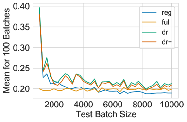
[Means] [Std. Dev.’s]

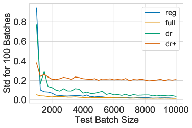
Figure 3: Figure 3: Mean of 100 MMD estimates at each batch size. Figure 3: Standard Deviation of 100 MMD estimates at each batch size

As discussed, when $\mathop{\mathbb{E}}[\Delta|X,Y]$ small, or $(Y,Z)$ highly correlated, or both, all estimators will be high variance. We train a model on the experiment 1 simulation using the none method and then study the mean and variance of dr, dr + (to study the effect of using the true $G_{W}$), reg (since it yielded better performance on mimic) and full (since this method is used to report the mmds in the tables). In this simulation, we are free to generate as many large batches of samples as needed. Keeping the model fixed, for each batch size between $1000$ and $10,000$ incrementing by $250$ we draw $100$ new batches of that size and estimate the mmd using each method. For each method, we report the mean (fig. 3) and standard deviation (fig. 3) of these estimates.

Notably, we cannot compute an actual ground-truth for the mmd of this model, but we could take the mean of the full estimate (no missingness) at the largest sample size of $10,000$ samples. This is about $0.2$. We see that the regression estimator stays closer to this number for all sample sizes relative to the dr methods. Interesting, for standard deviation, we see that the dr estimator is more well-behaved than the dr + estimator that uses the true $G_{W}$. This has also been observed for learned versus true propensity scores in treatment effect estimation and usually results from models learning less extreme probabilities than the true ones, trading some bias. In this case, there is not a substantial difference in estimated weights or in bias, but there is a large difference in variance. More investigation is required.

The main take-away from both plots is that the regression method seems more stable than dr and that $G_{W}$ may be the part of the dr estimator that is not being learned well. On the other hand the dr estimator may possibly be safer when it is unknown if it is easier to estimate $G_{W}$ or $m_{W}$. We recommend using all $3$ of the proposed estimators and comparing validation objectives.

Appendix C Full experiments

Table 4: Simulation. $\lambda=1$.

	none	obs	full	dr	dr +	reg	ip	ip +
tr mmd	$0.21\pm 0.04$	$0.05\pm 0.04$	$0.00\pm 0.01$	$0.00\pm 0.01$	$0.00\pm 0.01$	$0.01\pm 0.00$	$0.00\pm 0.00$	$0.00\pm 0.01$
tr acc	$0.89\pm 0.00$	$0.87\pm 0.00$	$0.86\pm 0.01$	$0.85\pm 0.01$	$0.84\pm 0.02$	$0.86\pm 0.00$	$0.84\pm 0.01$	$0.84\pm 0.01$
te acc	$0.67\pm 0.02$	$0.77\pm 0.02$	$0.80\pm 0.01$	$0.81\pm 0.02$	$0.81\pm 0.01$	$0.79\pm 0.02$	$0.82\pm 0.02$	$0.81\pm 0.00$

Table 5: Simulation. $\lambda=5$.

	none	obs	full	dr	dr +	reg	ip	ip +
tr mmd	$0.21\pm 0.04$	$0.03\pm 0.02$	$0.00\pm 0.01$	$0.00\pm 0.00$	$0.00\pm 0.0$	$0.00\pm 0.01$	$0.00\pm 0.0$	$0.00\pm 0.0$
tr acc	$0.89\pm 0.0$	$0.85\pm 0.02$	$0.84\pm 0.01$	$0.82\pm 0.01$	$0.78\pm 0.06$	$0.84\pm 0.00$	$0.81\pm 0.02$	$0.81\pm 0.03$
te acc	$0.67\pm 0.02$	$0.78\pm 0.02$	$0.83\pm 0.01$	$0.82\pm 0.02$	$0.77\pm 0.04$	$0.82\pm 0.01$	$0.81\pm 0.02$	$0.80\pm 0.01$

Table 6: mnist $\lambda=1$.

	none	obs	full	dr	dr +	reg	ip	ip +
tr mmd	$2.05\pm 0.18$	$0.02\pm 0.04$	$0.00\pm 0.01$	$0.00\pm 0.01$	$0.00\pm 0.01$	$0.00\pm 0.01$	$0.07\pm 0.12$.	$0.03\pm 0.06$
tr acc	$0.90\pm 0.01$	$0.74\pm 0.03$	$0.76\pm 0.01$	$0.77\pm 0.00$	$0.76\pm 0.01$	$0.76\pm 0.01$	$0.67\pm 0.16$	$0.68\pm 0.15$
te acc	$0.13\pm 0.01$	$0.63\pm 0.17$	$0.74\pm 0.01$	$0.72\pm 0.04$	$0.73\pm 0.01$	$0.73\pm 0.01$	$0.64\pm 0.14$	$0.61\pm 0.11$

Table 7: mnist $\lambda=5$.

	none	obs	full	dr	dr +	reg	ip	ip +
tr mmd	$2.05\pm 0.18$	$0.01\pm 0.02$	$0.00\pm 0.00$	$0.00\pm 0.00$	$0.00\pm 0.01$	$0.00\pm 0.01$	$0.01\pm 0.01$	$0.01\pm 0.02$
tr acc	$0.9\pm 0.01$	$0.66\pm 0.15$	$0.75\pm 0.01$	$0.65\pm 0.14$	$0.65\pm 0.13$	$0.75\pm 0.01$	$0.71\pm 0.08$	$0.60\pm 0.12$
te acc	$0.13\pm 0.01$	$0.65\pm 0.15$	$0.75\pm 0.01$	$0.73\pm 0.02$	$0.70\pm 0.09$	$0.75\pm 0.01$	$0.55\pm 0.3$	$0.60\pm 0.12$

Appendix D Failures of restricting to observed data

Proposition

There exist distributions on $(X,Y,\Delta,Z)$ such that

$$\exists h_{X}^{\star}\quad\text{s.t.}\quad h_{X}^{\star}\rotatebox[origin={c}]{90.0}{$\models$}Z|Y=y,\quad\text{but}\quad h_{X}^{\star}\rotatebox[origin={c}]{90.0}{$\not\models$}Z|Y=y,\Delta=1$$

and there exist distributions on $(X,Y,\Delta,Z)$ such that

$$\exists h_{X}^{\star}\quad\text{s.t.}\quad h_{X}^{\star}\rotatebox[origin={c}]{90.0}{$\models$}Z|Y=y,\Delta=1\quad\text{but}\quad h_{X}^{\star}\rotatebox[origin={c}]{90.0}{$\not\models$}Z|Y=y$$

First direction.

There exist distributions on $(X,Y,\Delta,Z)$ such that

$$\exists h_{X}^{\star}\quad\text{s.t.}\quad h_{X}^{\star}\rotatebox[origin={c}]{90.0}{$\models$}Z|Y=y,\quad\text{but}\quad h_{X}^{\star}\rotatebox[origin={c}]{90.0}{$\not\models$}Z|Y=y,\Delta=1$$

It suffices to illustrate this even when $Z,Y$ are not correlated. Consider

$$Y\sim\mathcal{N}(0,1),\quad Z\sim\mathcal{N}(0,\sigma_{Z}^{2}),\quad\epsilon_{X}\sim\mathcal{N}(0,\sigma_{X}^{2}),\quad X =[Y-Z+\epsilon_{X},Y+Z]$$

For $h_{X}^{\star}=(X_{1}+X_{2})$, we first show $h_{X}^{\star}\rotatebox[origin={c}]{90.0}{$\models$}Z|Y=y$. We have

$$h_{X}^{\star}|Y\sim\mathcal{N}(2Y,\sigma^{2}_{X})$$

and in particular $h_{X}^{\star}=2Y+\epsilon_{X}$. Given $Y=y$, the only randomness in $h_{X}^{\star}$ is due $\epsilon_{X}$. But $\epsilon_{X}$ is independent of the joint variable $(Z,Y)$ meaning $\epsilon_{X}\rotatebox[origin={c}]{90.0}{$\models$}Z|Y=y$ and therefore $h_{X}^{\star}\rotatebox[origin={c}]{90.0}{$\models$}Z|Y=y$.

We now construct $\Delta|(X,Y)$ such that $h_{X}^{\star}\rotatebox[origin={c}]{90.0}{$\not\models$}Z|Y=y,\Delta=1$. Let

$$\Delta=\text{OR}\Big{(}\mathbbm{1}\left[X_{1}+X_{2}<0\right],\mathbbm{1}\left[X_{2}-Y<0\right]\Big{)}.$$

Checking the condition

$$h_{X}^{\star}\rotatebox[origin={c}]{90.0}{$\not\models$}Z|Y=y,\Delta=1$$

(using definition of $h_{X}^{\star}$) is equivalent to checking

$$(X_{1}+X_{2})\rotatebox[origin={c}]{90.0}{$\not\models$}Z|Y=y,\Delta=1$$

(using definition of $\Delta$) is equivalent to checking

$$(X_{1}+X_{2})\rotatebox[origin={c}]{90.0}{$\not\models$}Z|Y=y,\text{OR}\Big{(}\mathbbm{1}\left[X_{1}+X_{2}<0\right],\mathbbm{1}\left[X_{2}-Y<0\right]\Big{)}=1$$

(using defintion of $X_{2}$) is equivalent to checking

$$(X_{1}+X_{2})\rotatebox[origin={c}]{90.0}{$\not\models$}Z|Y=y,\text{OR}\Big{(}\mathbbm{1}\left[X_{1}+X_{2}<0\right],\mathbbm{1}\left[Z<0\right]\Big{)}=1$$

To check that, we need to check if the distribution of $(X_{1}+X_{2})|Y=y,\Delta=1$ changes when conditioning on different events involving the random variable $Z$. For example, $\mathbbm{1}\left[Z<0\right]$ and $\mathbbm{1}\left[Z\geq 0\right]$:

1. $(X_{1}+X_{2})\quad|\quad Y=y,\text{OR}\Big{(}\mathbbm{1}\left[X_{1}+X_{2}<0\right],\mathbbm{1}\left[Z<0\right]\Big{)}=1,\mathbbm{1}\left[Z<0\right]=1$

2. $(X_{1}+X_{2})\quad|\quad Y=y,\text{OR}\Big{(}\mathbbm{1}\left[X_{1}+X_{2}<0\right],\mathbbm{1}\left[Z<0\right]\Big{)}=1,\mathbbm{1}\left[Z\geq 0\right]=1$.

We can show these two conditional variables differ in distribution simply by showing they differ in support. The first conditional variable can be full support because the event $\mathbbm{1}\left[Z<0\right]$ satisfies one of the OR conditions leaving the other condition $\mathbbm{1}\left[X_{1}+X_{2}<0\right]=\mathbbm{1}\left[h_{X}^{\star}<0\right]$ free to take either value. However, the second conditional variable needs $X_{1}+X_{2}=h_{X}^{\star}<0$ because $\mathbbm{1}\left[Z<0\right]$ is not satisfied (since we condition on $\mathbbm{1}\left[Z\geq 0\right]=1$) but the OR has to be $1$. These different supports imply the distributions differ. That the variables differ on two non-measure zero sets is enough to show dependence. Then $(X_{1}+X_{2})\rotatebox[origin={c}]{90.0}{$\not\models$}Z|Y=y,\Delta=1$ which means $h_{X}^{\star}\rotatebox[origin={c}]{90.0}{$\not\models$}Z|Y=y,\Delta=1$.

Second direction.

There exist distributions on $(X,Y,\Delta,Z)$ such that

$$\exists h_{X}^{\star}\quad\text{s.t.}\quad h_{X}^{\star}\rotatebox[origin={c}]{90.0}{$\models$}Z|Y=y,\Delta=1\quad\text{but}\quad h_{X}^{\star}\rotatebox[origin={c}]{90.0}{$\not\models$}Z|Y=y$$

Let the data be drawn as

$$Y\sim\mathcal{N}(0,1),\quad Z\sim\mathcal{B}(0.5),\quad X =[Y-Z,Y+Z]$$

Let $h_{X}^{\star}=\mathbbm{1}\left[X_{1}\geq 0\right]$. We first show $h_{X}^{\star}\rotatebox[origin={c}]{90.0}{$\not\models$}Z|Y=y$. We have

$$h_{X}^{\star} =\mathbbm{1}\left[X_{1}\geq 0\right]$$

$$=\mathbbm{1}\left[Y-Z\geq 0\right]$$

Given $Y=y$, we ask if the random variable $\mathbbm{1}\left[y-Z\geq 0\right]$ is independent of $Z$. To show dependence, we show that the random variable $\mathbbm{1}\left[y-Z\geq 0\right]$ changes in distribution when $Z$ takes on its two values:

1. $\mathbbm{1}\left[y-Z\geq 0\right]|Y=y,Z=0$

2. $\mathbbm{1}\left[y-Z\geq 0\right]|Y=y,Z=1$

Suppose $y\in(0,1)$. When $Z=0$ we have that $\mathbbm{1}\left[y-Z\geq 0\right]=1$ with probability one. When $Z=1$, we have $\mathbbm{1}\left[y-Z\geq 0\right]=0$ with probability one. Therefore the variables are dependent.

We now let $\Delta=\mathbbm{1}\left[X_{1}\geq 0\right]=\mathbbm{1}\left[Y-Z\geq 0\right]$ and show $h_{X}^{\star}\rotatebox[origin={c}]{90.0}{$\models$}Z|Y=y,\Delta=1$. Note that $\Delta(X,Y)=h_{X}^{\star}$. We ask whether

$$\mathbbm{1}\left[Y-Z\geq 0\right]\rotatebox[origin={c}]{90.0}{$\models$}Z|Y=y,\mathbbm{1}\left[Y-Z\geq 0\right]$$

The conditioning set fully determines the variable $\mathbbm{1}\left[Y-Z\geq 0\right]$ meaning it is a constant and is therefore independent of $Z$. Therefore $h_{X}^{\star}\rotatebox[origin={c}]{90.0}{$\models$}Z|Y=y,\Delta=1$ as desired.

Appendix E IP and outcome estimators

We review estimation of $\mathop{\mathbb{E}}[Z]$ under missingness. Two pieces of the data generation process can help, the missingness process $G_{W}$ and the conditional expectation $m_{W}$ of the missing variable:

$$G_{W}\triangleq\mathbb{E}[\Delta~{}|~{}X,Y],\quad\quad m_{W}\triangleq\mathbb{E}[Z~{}|~{}X,Y]$$

Inverse-weighting estimators use $G_{W}$ (Horvitz and Thompson, 1952; Binder, 1983; Robins et al., 1994; Van der Laan and Robins, 2003; Hernan and Robins, 2021)

$$\begin{split}\mathop{\mathbb{E}}[Z]&=\mathop{\mathbb{E}}_{X}\mathop{\mathbb{E}}_{Z|X}[Z]\\ &=\mathop{\mathbb{E}}_{X}\mathop{\mathbb{E}}_{Z|X}\Big{[}\frac{\mathop{\mathbb{E}}[\Delta|X]}{\mathop{\mathbb{E}}[\Delta|X]}Z\Big{]}\\ &=\mathop{\mathbb{E}}_{X}\mathop{\mathbb{E}}_{Z|X}\mathop{\mathbb{E}}_{\Delta|X}\Big{[}\frac{\Delta Z}{\mathop{\mathbb{E}}[\Delta|X]}\Big{]}\\ &=\mathop{\mathbb{E}}_{XZ\Delta}\Big{[}\frac{\Delta Z}{\mathop{\mathbb{E}}[\Delta|X]}\Big{]}\\ &=\mathop{\mathbb{E}}_{X\Delta Z}\Big{[}\frac{\Delta Z}{G_{W}}\Big{]}\\ &=\mathop{\mathbb{E}}_{X\Delta Z}\Big{[}\frac{\Delta\tilde{Z}}{G_{W}}\Big{]}\end{split}$$ (11)

This means we can estimate $\mathop{\mathbb{E}}[Z]$ provided that (1) ignorability and positivity hold and (2) $G_{W}$ is known. $G_{W}$ can be estimated by regressing $\Delta$ on $X$. Alternatively, standardization estimators use $m_{W}$ (Rubin, 1976; Schafer, 1997; Rubin, 2004; Pearl, 2009; Little and Rubin, 2019; Hernan and Robins, 2021):

$$\mathop{\mathbb{E}}[Z]=\mathop{\mathbb{E}}_{X}\Big{[}\mathop{\mathbb{E}}[Z|X]\Big{]}=\mathop{\mathbb{E}}_{X}\Big{[}\mathop{\mathbb{E}}[Z|X,\Delta=1]\Big{]}=\mathop{\mathbb{E}}[m_{W}]$$ (12)

The equality between the middle two terms means that $m_{W}$ can be estimated by regressing $\tilde{Z}$ on $X$ just on those samples where $\Delta=1$. The equality follows from the ignorability assumption $Z\rotatebox[origin={c}]{90.0}{$\models$}\Delta|X,Y$.

Appendix F DR estimator of mean of Z

The inverse weighting and regression estimators can be combined. Equation 3 defines the dr estimator of $\mathop{\mathbb{E}}[Z]$ by

$$\mathop{\mathbb{E}}[Z]=\mathop{\mathbb{E}}\Big{[}\frac{\Delta\tilde{Z}}{G_{W}}-\frac{\Delta-G_{W}}{G_{W}}m_{W}\Big{]}$$

Let us re-write this expectation until we see it equals $\mathop{\mathbb{E}}[Z]$ when $G$ or $m$ are correct.

$$\mathop{\mathbb{E}}\Big{[}\frac{\Delta\tilde{Z}}{G_{W}}-\frac{\Delta-G_{W}}{G_{W}}m_{W}\Big{]}$$

$$=\mathop{\mathbb{E}}\Big{[}\frac{\Delta Z}{G_{W}}-\frac{\Delta-G_{W}}{G_{W}}m_{W}\Big{]}$$

$$=\mathop{\mathbb{E}}\Big{[}Z+\frac{\Delta Z}{G_{W}}-Z-\frac{\Delta-G_{W}}{G_{W}}m_{W}\Big{]}$$

$$=\mathop{\mathbb{E}}\Big{[}Z+\frac{\Delta Z}{G_{W}}-\frac{G_{W}}{G_{W}}Z-\frac{\Delta-G_{W}}{G_{W}}m_{W}\Big{]}$$

$$=\mathop{\mathbb{E}}\Big{[}Z+\frac{\Delta-G_{W}}{G_{W}}Z-\frac{\Delta-G_{W}}{G_{W}}m_{W}\Big{]}$$

$$=\mathop{\mathbb{E}}\Big{[}Z+\frac{\Delta-G_{W}}{G_{W}}(Z-m_{W})\Big{]}$$

$$=\mathop{\mathbb{E}}\Big{[}Z\Big{]}+\mathop{\mathbb{E}}\Big{[}\frac{\Delta-G_{W}}{G_{W}}(Z-m_{W})\Big{]}$$

The first term is what we want, so we just have to check if the second term is $0$ when either $G$ or $m$ are correct. If $G$ is correct (regardless of $m$) then:

$$\mathop{\mathbb{E}}\Big{[}\frac{\Delta-G_{W}}{G_{W}}(Z-m_{W})\Big{]} =\mathop{\mathbb{E}}\Bigg{[}\mathop{\mathbb{E}}\Big{[}\frac{\Delta-G_{W}}{G_{W}}(Z-m_{W})\Big{|}X,Z\Big{]}\Bigg{]}$$

$$=\mathop{\mathbb{E}}\Bigg{[}\frac{\mathop{\mathbb{E}}[\Delta|X,Z]-G_{W}}{G_{W}}(Z-m_{W})\Bigg{]}$$

$$=\mathop{\mathbb{E}}\Bigg{[}\frac{\mathop{\mathbb{E}}[\Delta|X]-G_{W}}{G_{W}}(Z-m_{W})\Bigg{]}$$

$$=\mathop{\mathbb{E}}\Bigg{[}\frac{G_{W}-G_{W}}{G_{W}}(Z-m_{W})\Bigg{]}=0$$

When $m$ is correct (regardless of $G$):

$$\mathop{\mathbb{E}}\Big{[}\frac{\Delta-G_{W}}{G_{W}}(Z-m_{W})\Big{]} =\mathop{\mathbb{E}}\Bigg{[}\mathop{\mathbb{E}}\Big{[}\frac{\Delta-G_{W}}{G_{W}}(Z-m_{W})\Big{|}X,\Delta\Big{]}\Bigg{]}$$

$$=\mathop{\mathbb{E}}\Bigg{[}\frac{\Delta-G_{W}}{G_{W}}(\mathop{\mathbb{E}}[Z|X,\Delta]-m_{W})\Big{|}X,\Delta\Bigg{]}$$

$$=\mathop{\mathbb{E}}\Bigg{[}\frac{\Delta-G_{W}}{G_{W}}(\mathop{\mathbb{E}}[Z|X,\Delta]-\mathop{\mathbb{E}}[Z|X,\Delta=1])\Big{|}X,\Delta\Bigg{]}$$

$$=\mathop{\mathbb{E}}\Bigg{[}\frac{\Delta-G_{W}}{G_{W}}(\mathop{\mathbb{E}}[Z|X]-\mathop{\mathbb{E}}[Z|X])\Big{|}X,\Delta\Bigg{]}=0$$

Appendix G Deriving MMD estimators under missingness

G.1 Deriving the $G_{W}$-based re-weighted estimator

Here we start at the target quantity and derive the estimator. We give the derivation for $Z=1,Z^{\prime}=1$. The other cases are analogous.

$$\mathop{\mathbb{E}}_{P(X|Z=1)P(X^{\prime}|Z^{\prime}=1)}\Big{[}k_{XX^{\prime}}\Big{]}$$

$$=\int_{X,X^{\prime}}kP(X|Z=1)P(X^{\prime}|Z^{\prime}=1)dXdX^{\prime}$$

$$=\frac{1}{P(Z=1)}\frac{1}{P(Z^{\prime}=1)}\int_{X,X^{\prime}}kP(Z=1,X)P(Z^{\prime}=1,X^{\prime})dXdX^{\prime}$$

$$=\frac{1}{P(Z=1)}\frac{1}{P(Z^{\prime}=1)}\int_{X,X^{\prime}}kP(Z=1|X)P(Z^{\prime}=1|X)P(X)P(X^{\prime})dXdX^{\prime}$$

$$=\frac{1}{P(Z=1)}\frac{1}{P(Z^{\prime}=1)}\int_{X,X^{\prime}}k\mathop{\mathbb{E}}(Z=1|X)\mathop{\mathbb{E}}(Z^{\prime}=1|X)P(X)P(X^{\prime})dXdX^{\prime}$$

$$=\frac{1}{P(Z=1)}\frac{1}{P(Z^{\prime}=1)}\mathop{\mathbb{E}}_{\begin{subarray}{c}X,Z\\ X^{\prime},Z^{\prime}\end{subarray}}\Big{[}k\cdot Z\cdot Z^{\prime}\Big{]}$$

$$=\frac{1}{P(Z=1)}\frac{1}{P(Z^{\prime}=1)}\mathop{\mathbb{E}}_{\begin{subarray}{c}X,Z\\ X^{\prime},Z^{\prime}\end{subarray}}\Big{[}\frac{\mathop{\mathbb{E}}[\Delta|X]\mathop{\mathbb{E}}[\Delta^{\prime}|X^{\prime}]}{\mathop{\mathbb{E}}[\Delta|X]\mathop{\mathbb{E}}[\Delta^{\prime}|X^{\prime}]}k\cdot Z\cdot Z^{\prime}\Big{]}$$

$$=\frac{1}{P(Z=1)}\frac{1}{P(Z^{\prime}=1)}\mathop{\mathbb{E}}_{\begin{subarray}{c}X,\Delta,Z\\ X^{\prime},\Delta^{\prime},Z^{\prime}\end{subarray}}\Big{[}\frac{\Delta\Delta^{\prime}}{G_{W}G_{W^{\prime}}}k\cdot Z\cdot Z^{\prime}\Big{]}$$

G.2 Deriving the $m_{W}$-based standardization estimator

Here we start at the target quantity and derive the estimator. We give the derivation for $Z=1,Z^{\prime}=1$. The other cases are analogous.

$$\mathop{\mathbb{E}}_{P(X|Z=1)P(X^{\prime}|Z^{\prime}=1)}\Big{[}k_{XX^{\prime}}\Big{]}$$

$$=\int_{X,X^{\prime}}kP(X|Z=1)P(X^{\prime}|Z^{\prime}=1)dXdX^{\prime}$$

$$=\frac{1}{P(Z=1)}\frac{1}{P(Z^{\prime}=1)}\int_{X,X^{\prime}}kP(Z=1,X)P(Z^{\prime}=1,X^{\prime})dXdX^{\prime}$$

$$=\frac{1}{P(Z=1)}\frac{1}{P(Z^{\prime}=1)}\int_{X,X^{\prime}}kP(Z=1|X)P(Z^{\prime}=1|X)P(X)P(X^{\prime})dXdX^{\prime}$$

$$=\frac{1}{P(Z=1)}\frac{1}{P(Z^{\prime}=1)}\int_{X,X^{\prime}}k\mathop{\mathbb{E}}(Z=1|X)\mathop{\mathbb{E}}(Z^{\prime}=1|X)P(X)P(X^{\prime})dXdX^{\prime}$$

$$=\frac{1}{P(Z=1)}\frac{1}{P(Z^{\prime}=1)}\mathop{\mathbb{E}}_{X,X^{\prime}}\Big{[}m_{W}\cdot m_{W^{\prime}}\cdot k\Big{]}$$

G.3 Deriving the DR estimator

Here we start at the estimator and derive the target quantity. We give the derivation for $Z=1,Z^{\prime}=1$. The other cases are analogous.

$$\frac{1}{P(Z=1)}\frac{1}{P(Z^{\prime}=1)}\frac{1}{N(N-1)}\sum_{i\neq j}\Big{[}\frac{\Delta_{ij}\tilde{Z}_{ij}}{G_{ij}}k_{ij}-\frac{\Delta_{ij}-G_{ij}}{G_{ij}}m_{ij}k_{ij}\Big{]}$$

$$\approx\frac{1}{P(Z=1)}\frac{1}{P(Z^{\prime}=1)}\mathop{\mathbb{E}}_{\begin{subarray}{c}X,\Delta,Z\\ X^{\prime},\Delta^{\prime},Z^{\prime}\end{subarray}}\Big{[}\frac{\Delta\Delta^{\prime}\tilde{Z}\tilde{Z}^{\prime}}{G_{W}G_{W^{\prime}}}k-\frac{\Delta\Delta^{\prime}-G_{W}G_{W^{\prime}}}{G_{W}G_{W^{\prime}}}m_{W}m_{W^{\prime}}k\Big{]}$$

$$=\frac{1}{P(Z=1)}\frac{1}{P(Z^{\prime}=1)}\mathop{\mathbb{E}}_{\begin{subarray}{c}X,\Delta,Z\\ X^{\prime},\Delta^{\prime},Z^{\prime}\end{subarray}}\Big{[}\frac{\Delta\Delta^{\prime}ZZ^{\prime}}{G_{W}G_{W^{\prime}}}k-\frac{\Delta\Delta^{\prime}-G_{W}G_{W^{\prime}}}{G_{W}G_{W^{\prime}}}m_{W}m_{W^{\prime}}k\Big{]}$$

$$=\frac{1}{P(Z=1)}\frac{1}{P(Z^{\prime}=1)}\mathop{\mathbb{E}}_{\begin{subarray}{c}X,\Delta,Z\\ X^{\prime},\Delta^{\prime},Z^{\prime}\end{subarray}}\Big{[}ZZ^{\prime}k+\frac{\Delta\Delta^{\prime}}{G_{W}G_{W^{\prime}}}ZZ^{\prime}k-ZZ^{\prime}k-\frac{\Delta\Delta^{\prime}-G_{W}G_{W^{\prime}}}{G_{W}G_{W^{\prime}}}m_{W}m_{W^{\prime}}k\Big{]}$$

$$=\frac{1}{P(Z=1)}\frac{1}{P(Z^{\prime}=1)}\mathop{\mathbb{E}}_{\begin{subarray}{c}X,\Delta,Z\\ X^{\prime},\Delta^{\prime},Z^{\prime}\end{subarray}}\Big{[}ZZ^{\prime}k+\frac{\Delta\Delta^{\prime}}{G_{W}G_{W^{\prime}}}ZZ^{\prime}k-\frac{G_{W}G_{W^{\prime}}}{G_{W}G_{W^{\prime}}}ZZ^{\prime}k-\frac{\Delta\Delta^{\prime}-G_{W}G_{W^{\prime}}}{G_{W}G_{W^{\prime}}}m_{W}m_{W^{\prime}}k\Big{]}$$

$$=\frac{1}{P(Z=1)}\frac{1}{P(Z^{\prime}=1)}\mathop{\mathbb{E}}_{\begin{subarray}{c}X,\Delta,Z\\ X^{\prime},\Delta^{\prime},Z^{\prime}\end{subarray}}\Big{[}ZZ^{\prime}k+\frac{\Delta\Delta^{\prime}-G_{W}G_{W^{\prime}}}{G_{W}G_{W^{\prime}}}ZZ^{\prime}k-\frac{\Delta\Delta^{\prime}-G_{W}G_{W^{\prime}}}{G_{W}G_{W^{\prime}}}m_{W}m_{W^{\prime}}k\Big{]}$$

$$=\frac{1}{P(Z=1)}\frac{1}{P(Z^{\prime}=1)}\mathop{\mathbb{E}}_{\begin{subarray}{c}X,\Delta,Z\\ X^{\prime},\Delta^{\prime},Z^{\prime}\end{subarray}}\Big{[}ZZ^{\prime}k+\frac{\Delta\Delta^{\prime}-G_{W}G_{W^{\prime}}}{G_{W}G_{W^{\prime}}}\Big{(}ZZ^{\prime}-m_{W}m_{W^{\prime}}\Big{)}k\Big{]}$$

$$=\frac{1}{P(Z=1)}\frac{1}{P(Z^{\prime}=1)}\mathop{\mathbb{E}}_{\begin{subarray}{c}X,\Delta,Z\\ X^{\prime},\Delta^{\prime},Z^{\prime}\end{subarray}}\Big{[}ZZ^{\prime}k\Big{]}+\frac{1}{P(Z=1)}\frac{1}{P(Z^{\prime}=1)}\mathop{\mathbb{E}}_{\begin{subarray}{c}X,\Delta,Z\\ X^{\prime},\Delta^{\prime},Z^{\prime}\end{subarray}}\Big{[}\frac{\Delta\Delta^{\prime}-G_{W}G_{W^{\prime}}}{G_{W}G_{W^{\prime}}}\Big{(}ZZ^{\prime}-m_{W}m_{W^{\prime}}\Big{)}k\Big{]}$$

Our estimator equals two terms. We first show that the first term equals the desired quantity, and then show the second term equals 0 when either auxiliary model is correct.

$$\frac{1}{P(Z=1)}\frac{1}{P(Z^{\prime}=1)}\mathop{\mathbb{E}}_{\begin{subarray}{c}X,\Delta,Z\\ X^{\prime},\Delta^{\prime},Z^{\prime}\end{subarray}}\Big{[}ZZ^{\prime}k\Big{]} =\frac{1}{P(Z=1)}\frac{1}{P(Z^{\prime}=1)}\mathop{\mathbb{E}}_{X,X^{\prime}}\Big{[}k\mathop{\mathbb{E}}[Z,Z^{\prime}|X,X^{\prime}]\Big{]}$$

$$=\frac{1}{P(Z=1)}\frac{1}{P(Z^{\prime}=1)}\mathop{\mathbb{E}}_{X,X^{\prime}}\Big{[}kP(Z=1,Z^{\prime}=1|X,X^{\prime})\Big{]}$$

$$=\frac{1}{P(Z=1)}\frac{1}{P(Z^{\prime}=1)}\int_{X,X^{\prime}}kP(Z=1,Z^{\prime}=1|X,X^{\prime})P(X,X^{\prime})dXdX^{\prime}$$

$$=\frac{1}{P(Z=1)}\frac{1}{P(Z^{\prime}=1)}\int_{X,X^{\prime}}kP(Z=1|X)P(Z^{\prime}=1|X)P(X)P(X^{\prime})dXdX^{\prime}$$

$$=\frac{1}{P(Z=1)}\frac{1}{P(Z^{\prime}=1)}\int_{X,X^{\prime}}kP(Z=1,X)P(Z^{\prime}=1,X^{\prime})dXdX^{\prime}$$

$$=\frac{1}{P(Z=1)}\frac{1}{P(Z^{\prime}=1)}\int_{X,X^{\prime}}kP(Z=1,X)P(Z^{\prime}=1,X^{\prime})dXdX^{\prime}$$

$$=\int_{X,X^{\prime}}kP(X|Z=1)P(X^{\prime}|Z^{\prime}=1)dXdX^{\prime}$$

$$=\mathop{\mathbb{E}}_{P(X|Z=1)P(X^{\prime}|Z^{\prime}=1)}\Big{[}k\Big{]}$$

That’s the expectation we want missing just the $P(Z=1)$ constants, so now we should show the next term is $0$ when either $m$ or $G$ are correct. When $G$ correct:

$$\mathop{\mathbb{E}}_{\begin{subarray}{c}X,\Delta,Z\\ X^{\prime},\Delta^{\prime},Z^{\prime}\end{subarray}}\Big{[}\frac{\Delta\Delta^{\prime}-G_{W}G_{W^{\prime}}}{G_{W}G_{W^{\prime}}}\Big{(}ZZ^{\prime}-m_{W}m_{W^{\prime}}\Big{)}k\Big{]} =\mathop{\mathbb{E}}_{\begin{subarray}{c}X,Z\\ X^{\prime},Z^{\prime}\end{subarray}}\Big{[}\frac{\mathop{\mathbb{E}}[\Delta\Delta^{\prime}|X,X^{\prime},Y,Z^{\prime}]-G_{W}G_{W^{\prime}}}{G_{W}G_{W^{\prime}}}\Big{(}ZZ^{\prime}-m_{W}m_{W^{\prime}}\Big{)}k\Big{]}$$

$$=\mathop{\mathbb{E}}_{\begin{subarray}{c}X,Z\\ X^{\prime},Z^{\prime}\end{subarray}}\Big{[}\frac{\mathop{\mathbb{E}}[\Delta\Delta^{\prime}|X,X^{\prime}]-G_{W}G_{W^{\prime}}}{G_{W}G_{W^{\prime}}}\Big{(}ZZ^{\prime}-m_{W}m_{W^{\prime}}\Big{)}k\Big{]}$$

$$=\mathop{\mathbb{E}}_{\begin{subarray}{c}X,Z\\ X^{\prime},Z^{\prime}\end{subarray}}\Big{[}\frac{\mathop{\mathbb{E}}[\Delta|X]\mathop{\mathbb{E}}[\Delta^{\prime}|X^{\prime}]-G_{W}G_{W^{\prime}}}{G_{W}G_{W^{\prime}}}\Big{(}ZZ^{\prime}-m_{W}m_{W^{\prime}}\Big{)}k\Big{]}$$

$$=\mathop{\mathbb{E}}_{\begin{subarray}{c}X,Z\\ X^{\prime},Z^{\prime}\end{subarray}}\Big{[}\frac{G_{W}G_{W^{\prime}}-G_{W}G_{W^{\prime}}}{G_{W}G_{W^{\prime}}}\Big{(}ZZ^{\prime}-m_{W}m_{W^{\prime}}\Big{)}k\Big{]}=0$$

Likewise, when $m$ correct:

$$\mathop{\mathbb{E}}_{\begin{subarray}{c}X,\Delta,Z\\ X^{\prime},\Delta^{\prime},Z^{\prime}\end{subarray}}\Big{[}\frac{\Delta\Delta^{\prime}-G_{W}G_{W^{\prime}}}{G_{W}G_{W^{\prime}}}\Big{(}ZZ^{\prime}-m_{W}m_{W^{\prime}}\Big{)}k\Big{]}$$

$$=\mathop{\mathbb{E}}_{\begin{subarray}{c}X,\Delta\\ X^{\prime},\Delta^{\prime}\end{subarray}}\Big{[}\frac{\Delta\Delta^{\prime}-G_{W}G_{W^{\prime}}}{G_{W}G_{W^{\prime}}}\Big{(}\mathop{\mathbb{E}}[ZZ^{\prime}|X,X^{\prime},\Delta,\Delta^{\prime}]-m_{W}m_{W^{\prime}}\Big{)}k\Big{]}$$

$$=\mathop{\mathbb{E}}_{\begin{subarray}{c}X,\Delta\\ X^{\prime},\Delta^{\prime}\end{subarray}}\Big{[}\frac{\Delta\Delta^{\prime}-G_{W}G_{W^{\prime}}}{G_{W}G_{W^{\prime}}}\Big{(}\mathop{\mathbb{E}}[Z|X,\Delta]\mathop{\mathbb{E}}[Z^{\prime}|X^{\prime},\Delta^{\prime}]-m_{W}m_{W^{\prime}}\Big{)}k\Big{]}$$

$$=\mathop{\mathbb{E}}_{\begin{subarray}{c}X,\Delta\\ X^{\prime},\Delta^{\prime}\end{subarray}}\Big{[}\frac{\Delta\Delta^{\prime}-G_{W}G_{W^{\prime}}}{G_{W}G_{W^{\prime}}}\Big{(}\mathop{\mathbb{E}}[Z|X,\Delta]\mathop{\mathbb{E}}[Z^{\prime}|X^{\prime},\Delta^{\prime}]-\mathop{\mathbb{E}}[Z|X,\Delta=1]\mathop{\mathbb{E}}[Z^{\prime}|X^{\prime},\Delta^{\prime}=1]\Big{)}k\Big{]}$$

$$=\mathop{\mathbb{E}}_{\begin{subarray}{c}X,\Delta\\ X^{\prime},\Delta^{\prime}\end{subarray}}\Big{[}\frac{\Delta\Delta^{\prime}-G_{W}G_{W^{\prime}}}{G_{W}G_{W^{\prime}}}\Big{(}\mathop{\mathbb{E}}[Z|X]\mathop{\mathbb{E}}[Z^{\prime}|X^{\prime}]-\mathop{\mathbb{E}}[Z|X]\mathop{\mathbb{E}}[Z^{\prime}|X^{\prime}]\Big{)}k\Big{]}=0$$

The proof for the other two terms is analogous but with using $\overline{Z}=(1-Z)$ instead of $Z$ and $\overline{m}=1-m$ when conditioning on $Z=0$.

Appendix H kernel mmd between joint and product of marginals

Continuous nuisances.

In this work we study binary nuisance. We can instead measure the mmd between joint $p(h_{X},Z)$ and product of marginals $p(h_{X})P(Z)$, which allows for continuous nuisance.

The above formulation of mmd between $h_{X}|Z=1$ and $h_{X}|Z=0$ relied on optimizing with respect to $h$ only: $P(Z)$ is constant in the optimization so the distance between conditionals specifies the distance between the product of marginals and joint and thus the dependence. However, considering the more general case of mmd between $P(h_{X},Z)$ and $P(h_{X})P(Z)$ has the advantage that is not necessary to consider a finite set of conditioning values for $Z$. That means the mmd can be extended to continuous nuisance $Z$. Let $X::Z$ denote the concatenation of $X$ and $Z$. The more general formulation is:

$$\mathbb{E}_{\begin{subarray}{c}(X,Z)\sim P(X,Z)\\ (X^{\prime},Z^{\prime})\sim P(X,Z)\end{subarray}} \Bigg{[}k\Big{(}X\cat\cat Z,X^{\prime}\cat\cat Z^{\prime}\Big{)}\Bigg{]}+\mathbb{E}_{\begin{subarray}{c}(X,Z)\sim P(X)P(Z)\\ (X^{\prime},Z^{\prime})\sim P(X^{\prime})P(Z^{\prime})\end{subarray}}\Bigg{[}k\Big{(}X\cat\cat Z,X^{\prime}\cat\cat Z^{\prime}\Big{)}\Bigg{]}$$

$$-2\mathbb{E}_{\begin{subarray}{c}(X,Z)\sim P(X,Z)\\ (X^{\prime},Z^{\prime})\sim P(X^{\prime})P(Z^{\prime})\end{subarray}}\Bigg{[}k\Big{(}X\cat\cat Z,X^{\prime}\cat\cat Z^{\prime}\Big{)}\Bigg{]}$$

This leads to the following estimator:

$$\mathbb{E}_{\begin{subarray}{c}P(X,Z)\\ P(X^{\prime},Z^{\prime})\end{subarray}}\Bigg{[}k\Big{(}X\cat\cat Z,X^{\prime}\cat\cat Z^{\prime}\Big{)}\Bigg{]} =\mathbb{E}\Bigg{[}\frac{\Delta\Delta^{\prime}k(X\cat\cat Z,X^{\prime}\cat\cat Z^{\prime})}{G_{WW^{\prime}}}-\frac{\Delta\Delta^{\prime}-G_{WW^{\prime}}}{G_{WW^{\prime}}}\mathop{\mathbb{E}}[k|X,X^{\prime}]\Bigg{]}$$

and

$$\mathbb{E}_{\begin{subarray}{c}P(X)P(Z)\\ P(X^{\prime})P(Z^{\prime})\end{subarray}} \Bigg{[}k\Big{(}X\cat\cat Z,X^{\prime}\cat\cat Z^{\prime}\Big{)}\Bigg{]}$$

$$=\mathbb{E}_{\begin{subarray}{c}P(X_{1})P(X_{2},Z_{2})\\ P(X_{3})P(X_{4},Z_{4})\end{subarray}}\Bigg{[}k\Big{(}X_{1}\cat\cat Z_{2},X_{3}\cat\cat Z_{4}\Big{)}\Bigg{]}$$

$$=\mathbb{E}\Bigg{[}\frac{\Delta\Delta^{\prime}k(X_{1}\cat\cat Z_{2},X_{3}\cat\cat Z_{4})}{G_{X_{1}X_{3}}}-\frac{\Delta\Delta^{\prime}-G_{X_{1}X_{3}}}{G_{X_{1}X_{3}}}\mathop{\mathbb{E}}[k(X_{1}\cat\cat Z_{2},X_{3}\cat\cat Z_{4})|X_{1},X_{3}]\Bigg{]}$$

and

$$\mathbb{E}_{\begin{subarray}{c}P(X,Z)\\ P(X^{\prime})P(Z^{\prime})\end{subarray}} \Bigg{[}k\Big{(}X\cat\cat Z,X^{\prime}\cat\cat Z^{\prime}\Big{)}\Bigg{]}$$

$$=\mathbb{E}_{\begin{subarray}{c}P(X_{1},Z_{1})\\ P(X_{2})P(X_{3},Z_{3})\end{subarray}}\Bigg{[}k\Big{(}X_{1}\cat\cat Z_{1},X_{2}\cat\cat Z_{3}\Big{)}\Bigg{]}$$

$$=\mathbb{E}\Bigg{[}\frac{\Delta\Delta^{\prime}k(X_{1}\cat\cat Z_{1},X_{2}\cat\cat Z_{3})}{G_{X_{1}X_{3}}}-\frac{\Delta\Delta^{\prime}-G_{X_{1}X_{3}}}{G_{X_{1}X_{3}}}\mathop{\mathbb{E}}[k(X_{1}\cat\cat Z_{1},X_{2}\cat\cat Z_{3})|X_{1},X_{3}]\Bigg{]}$$

The challenging part of applying this estimator is that now instead of one function $m_{W}$ we have three functions, each of which estimates the mean of $k$ under a different sampling distribution. Moreover, these conditional expectations depend on the current representation $h_{X}$. This means they must be updated each time $h$ changes.

References

- Ahmed et al. (2020) Faruk Ahmed, Yoshua Bengio, Harm van Seijen, and Aaron Courville. Systematic generalisation with group invariant predictions. In International Conference on Learning Representations, 2020.
- Arjovsky et al. (2019) Martin Arjovsky, Léon Bottou, Ishaan Gulrajani, and David Lopez-Paz. Invariant risk minimization. arXiv preprint arXiv:1907.02893, 2019.
- Bang and Robins (2005) Heejung Bang and James M Robins. Doubly robust estimation in missing data and causal inference models. Biometrics, 61(4):962–973, 2005.
- Binder (1983) David A Binder. On the variances of asymptotically normal estimators from complex surveys. International Statistical Review/Revue Internationale de Statistique, pages 279–292, 1983.
- Chen et al. (2018) Irene Chen, Fredrik D Johansson, and David Sontag. Why is my classifier discriminatory? arXiv preprint arXiv:1805.12002, 2018.
- Creager et al. (2021) Elliot Creager, Jörn-Henrik Jacobsen, and Richard Zemel. Environment inference for invariant learning. In International Conference on Machine Learning, pages 2189–2200. PMLR, 2021.
- Davidian (2005) Marie Davidian. Double robustness in estimation of causal treatment effects, 2005.
- Geirhos et al. (2020) Robert Geirhos, Jörn-Henrik Jacobsen, Claudio Michaelis, Richard Zemel, Wieland Brendel, Matthias Bethge, and Felix A Wichmann. Shortcut learning in deep neural networks. Nature Machine Intelligence, 2(11):665–673, 2020.
- Goldberger et al. (2000) Ary L Goldberger, Luis AN Amaral, Leon Glass, Jeffrey M Hausdorff, Plamen Ch Ivanov, Roger G Mark, Joseph E Mietus, George B Moody, Chung-Kang Peng, and H Eugene Stanley. Physiobank, physiotoolkit, and physionet: components of a new research resource for complex physiologic signals. circulation, 101(23):e215–e220, 2000.
- Goodfellow et al. (2013) Ian J. Goodfellow, David Warde-Farley, Pascal Lamblin, Vincent Dumoulin, Mehdi Mirza, Razvan Pascanu, James Bergstra, Frédéric Bastien, and Yoshua Bengio. Pylearn2: a machine learning research library. arXiv preprint arXiv:1308.4214, 2013. URL http://arxiv.org/abs/1308.4214.
- Gretton et al. (2005) Arthur Gretton, Olivier Bousquet, Alex Smola, and Bernhard Schölkopf. Measuring statistical dependence with hilbert-schmidt norms. In International conference on algorithmic learning theory, pages 63–77. Springer, 2005.
- Gretton et al. (2012) Arthur Gretton, Karsten M Borgwardt, Malte J Rasch, Bernhard Schölkopf, and Alexander Smola. A kernel two-sample test. The Journal of Machine Learning Research, 13(1):723–773, 2012.
- Gulrajani and Lopez-Paz (2020) Ishaan Gulrajani and David Lopez-Paz. In search of lost domain generalization. arXiv preprint arXiv:2007.01434, 2020.
- Hébert-Johnson et al. (2018) Ursula Hébert-Johnson, Michael Kim, Omer Reingold, and Guy Rothblum. Multicalibration: Calibration for the (computationally-identifiable) masses. In International Conference on Machine Learning, pages 1939–1948. PMLR, 2018.
- Hernan and Robins (2021) Miguel A. Hernan and James M. Robins. Causal Inference: What If. Chapman & Hall/CRC, 1st edition, 2021.
- Horvitz and Thompson (1952) Daniel G Horvitz and Donovan J Thompson. A generalization of sampling without replacement from a finite universe. Journal of the American statistical Association, 47(260):663–685, 1952.
- Johnson et al. (2016) Alistair EW Johnson, Tom J Pollard, Lu Shen, H Lehman Li-wei, Mengling Feng, Mohammad Ghassemi, Benjamin Moody, Peter Szolovits, Leo Anthony Celi, and Roger G Mark. Mimic-iii, a freely accessible critical care database. Scientific data, 3:160035, 2016.
- Kang and Schafer (2007) Joseph DY Kang and Joseph L Schafer. Demystifying double robustness: A comparison of alternative strategies for estimating a population mean from incomplete data. Statistical science, pages 523–539, 2007.
- Krueger et al. (2021) David Krueger, Ethan Caballero, Joern-Henrik Jacobsen, Amy Zhang, Jonathan Binas, Dinghuai Zhang, Remi Le Priol, and Aaron Courville. Out-of-distribution generalization via risk extrapolation (rex). In International Conference on Machine Learning, pages 5815–5826. PMLR, 2021.
- Lahoti et al. (2020) Preethi Lahoti, Alex Beutel, Jilin Chen, Kang Lee, Flavien Prost, Nithum Thain, Xuezhi Wang, and Ed H Chi. Fairness without demographics through adversarially reweighted learning. arXiv preprint arXiv:2006.13114, 2020.
- Little and Rubin (2019) Roderick JA Little and Donald B Rubin. Statistical analysis with missing data, volume 793. John Wiley & Sons, 2019.
- Liu et al. (2021) Evan Z Liu, Behzad Haghgoo, Annie S Chen, Aditi Raghunathan, Pang Wei Koh, Shiori Sagawa, Percy Liang, and Chelsea Finn. Just train twice: Improving group robustness without training group information. In International Conference on Machine Learning, pages 6781–6792. PMLR, 2021.
- Makar et al. (2021) Maggie Makar, Ben Packer, Dan Moldovan, Davis Blalock, Yoni Halpern, and Alexander D’Amour. Causally-motivated shortcut removal using auxiliary labels. arXiv preprint arXiv:2105.06422, 2021.
- Namkoong and Duchi (2016) Hongseok Namkoong and John C Duchi. Stochastic gradient methods for distributionally robust optimization with f-divergences. In NeurIPS, volume 29, pages 2208–2216, 2016.
- Obermeyer et al. (2019) Ziad Obermeyer, Brian Powers, Christine Vogeli, and Sendhil Mullainathan. Dissecting racial bias in an algorithm used to manage the health of populations. Science, 366(6464):447–453, 2019.
- Pearl (2009) Judea Pearl. Causality. Cambridge university press, 2009.
- Peters et al. (2016) Jonas Peters, Peter Bühlmann, and Nicolai Meinshausen. Causal inference by using invariant prediction: identification and confidence intervals. Journal of the Royal Statistical Society. Series B (Statistical Methodology), pages 947–1012, 2016.
- Puli et al. (2022) Aahlad Manas Puli, Lily H Zhang, Eric Karl Oermann, and Rajesh Ranganath. Out-of-distribution generalization in the presence of nuisance-induced spurious correlations. In International Conference on Learning Representations, 2022. URL https://openreview.net/forum?id=12RoR2o32T.
- Robins et al. (1994) James M Robins, Andrea Rotnitzky, and Lue Ping Zhao. Estimation of regression coefficients when some regressors are not always observed. Journal of the American statistical Association, 89(427):846–866, 1994.
- Robins and Rotnitzky (2001) J.M. Robins and A G Rotnitzky. Comment on the bickel and kwon article, ’inference for semiparametric models: Some questions and an answer’. Statistica Sinica, 11:920–936, 01 2001.
- Rubin (1976) Donald B Rubin. Inference and missing data. Biometrika, 63(3):581–592, 1976.
- Rubin (2004) Donald B Rubin. Multiple imputation for nonresponse in surveys, volume 81. John Wiley & Sons, 2004.
- Sagawa et al. (2020) Shiori Sagawa, Aditi Raghunathan, Pang Wei Koh, and Percy Liang. An investigation of why overparameterization exacerbates spurious correlations. In International Conference on Machine Learning, pages 8346–8356. PMLR, 2020.
- Schafer (1997) Joseph L Schafer. Analysis of incomplete multivariate data. CRC press, 1997.
- Szabó and Sriperumbudur (2017) Zoltán Szabó and Bharath K Sriperumbudur. Characteristic and universal tensor product kernels. J. Mach. Learn. Res., 18:233–1, 2017.
- Van der Laan and Robins (2003) Mark J Van der Laan and James M Robins. Unified methods for censored longitudinal data and causality. Springer Science & Business Media, 2003.
- Veitch et al. (2021) Victor Veitch, Alexander D’Amour, Steve Yadlowsky, and Jacob Eisenstein. Counterfactual invariance to spurious correlations in text classification. Advances in Neural Information Processing Systems, 34, 2021.
- Wang et al. (2020) Serena Wang, Wenshuo Guo, Harikrishna Narasimhan, Andrew Cotter, Maya Gupta, and Michael I Jordan. Robust optimization for fairness with noisy protected groups. arXiv preprint arXiv:2002.09343, 2020.
- WHO (2004) Expert Consultation WHO. Appropriate body-mass index for Asian populations and its implications for policy and intervention strategies. Lancet (London, England), 363(9403):157–163, 2004.