Generating Diverse 3D Reconstructions from a Single Occluded Face Image

Abstract

Occlusions are a common occurrence in unconstrained face images. Single image 3D reconstruction from such face images often suffers from corruption due to the presence of occlusions. Furthermore, while a plurality of 3D reconstructions is plausible in the occluded regions, existing approaches are limited to generating only a single solution. To address both of these challenges, we present Diverse3DFace, which is specifically designed to simultaneously generate a diverse and realistic set of 3D reconstructions from a single occluded face image. It comprises three components; a global+local shape fitting process, a graph neural network-based mesh VAE, and a determinantal point process based diversity-promoting iterative optimization procedure. Quantitative and qualitative comparisons of 3D reconstruction on occluded faces show that Diverse3DFace can estimate 3D shapes that are consistent with the visible regions in the target image while exhibiting high, yet realistic, levels of diversity in the occluded regions. On face images occluded by masks, glasses, and other random objects, Diverse3DFace generates a distribution of 3D shapes having $\sim$50% higher diversity on the occluded regions compared to the baselines. Moreover, our closest sample to the ground truth has $\sim$40% lower MSE than the singular reconstructions by existing approaches. Code and data available at: https://github.com/human-analysis/diverse3dface

1 Introduction

Single image-based 3D face reconstruction has improved significantly in recent years [56, 10]. This includes advances in statistical models [3, 28, 22, 29] as well as neural network-based models [40, 42, 35, 48, 12, 13, 41, 47, 43]. However, facial occlusions remain a significant challenge to this task. In-the-wild face images often come with several forms of occlusions and unless dealt with explicitly, often lead to erroneous 3D reconstruction in terms of shape, expression, pose, etc. [10, 9, 44].

3D reconstruction of partially occluded faces presents two main challenges. First, 3D reconstruction models need to selectively use features from the visible regions while ignoring those from the occluded parts. Failure to do so, either implicitly or explicitly, will lead to poor 3D reconstructions with an incorrect pose, expression, or both. Second, there could be a distribution of 3D reconstructions that are consistent with the visible parts in the image yet diverse on the occluded parts. Failure to account for all such modes limits the utility of 3D reconstruction models. Addressing these two challenges is the primary goal of this paper.

Existing 3D face reconstruction solutions, however, are ill-equipped to overcome both of these challenges simultaneously. From a reconstruction perspective, a majority of the approaches that reconstruct 3D faces from a single image restrict themselves to fully-visible face images. And, even those that explicitly account for facial occlusions [44, 9], do so only in a holistic manner using a global model that implicitly uses features from the occluded regions as well. This form of global model-based fitting can introduce errors (see Fig. 1) in the pose and expression of the 3D reconstruction, especially when large portions of the face are occluded. From a diversity perspective, existing approaches are, by design, limited to only generating a single plausible 3D reconstruction. However, in many practical applications, for a single occluded face image, it is desirable to generate multiple reconstructions that are consistent on the visible parts of the face, while spanning a diverse yet realistic set of reconstructions on the occluded parts (see Fig. 1). While the concept of generating diverse solutions has been explored in other contexts such as image generation [11], image completion [53], super-resolution [1] and trajectory forecasting [51], they have not been explored for monocular 3D face reconstruction of occluded faces.

In this paper, we propose Diverse3DFace which is designed to simultaneously yield a diverse, yet plausible, set of 3D reconstructions from a single occluded face image. Diverse3DFace consists of three modules: a global + local shape fitting process, a graph neural network based variational autoencoder (Mesh-VAE), and a Determinantal Point Process (DPP) [21] based iterative optimization procedure. The global + local shape fitting process affords robustness against large occlusions by decoupling shape fitting on the visible regions from that of the occluded regions. The Mesh-VAE enables to learn a distribution over a compact latent space over the different factors of variation in the 3D shapes of faces. And, the DPP-based iterative optimization procedure enables us to sample from the latent space of the Mesh-VAE and optimize them to generate a diverse set of reconstructions spanning the different modes of the latent space. Our specific contributions in this paper are:

– We propose Diverse3DFace, a simple yet effective diversity promoting 3D face reconstruction approach that generates multiple plausible 3D reconstructions corresponding to a single occluded face image.

– For robustness to occlusions, we propose a global + local PCA model based shape fitting that disentangles the fitting on each facial component from the others. The models are learned from a dataset of FLAME [22] registered 3D meshes. During inference, the local perturbations on various facial components are added on top of a coarse global fit to generate the final detailed fitting.

– We employ a DPP [21] based diversity loss in the context of generating diverse 3D reconstructions of faces. We define the quality and similarity terms in the DPP kernel to maximize diversity while remaining in the space of realistic 3D head shapes.

– We conduct extensive qualitative and quantitative experiments to show the efficacy of the proposed approach in generating 3D reconstructions that are faithful to the visible face while simultaneously capturing multiple diverse modes on the occluded parts. The solution from Diverse3DFace that is closest to the ground truth is on average 30-50% better than the unique solutions of the baselines [12, 22] in terms of per-vertex $\ell_{2}$-error.

2 Related Work

Single Image 3D Face Reconstruction: Blanz and Vetter [3] proposed the first 3DMM model of human faces. Since then, such models have grown to include complex pose and expression modalities in 3D faces [28, 14]. Li et al. [22] proposed FLAME that models the full human head and allows non-linear control over joint poses to generate articulated expressive head instances. Many recent approaches adopted neural networks to model higher-order complexities in the shape and expression spaces [40, 35, 36, 42, 41, 43, 30, 19, 33, 48, 12]. A few methods took a hybrid approach of fitting a non-linear neural network model to the target image to generate detailed 3D reconstructions [13, 50]. More recently, advances in graph neural networks [20, 45, 8, 25] have propagated using graph convolution operations to directly learn non-linear representation on a mesh surface while preserving the mesh topology [31, 4, 54]. Though these advances have significantly improved the modeling capabilities of 3D face reconstruction approaches, they are still limited when handling occlusions in face images.

On the other hand, a few approaches are explicitly designed to handle occlusions [44, 9, 18]. Tran et al. [44] trained a neural network to regress a robust foundation shape from a masked face image, over which a detailed bump map is added later. And, Egger et al. [9] simultaneously optimized an occlusion mask and the model parameters from an occluded image. However, these approaches rely on a global model to account for the entire face, including the occluded parts, which is sub-optimal as the lack of information from such parts needs to be countered using strong regularization. Moreover, they are limited to reconstructing a singular 3D solution without considering the plurality of solutions that can explain the occluded regions. In contrast, we address the dual problems of robustness and lack of uniqueness through a multistage approach that disentangles fitting on the visible regions from diversity modeling on the occluded ones.

Diversity Promoting Generative Models: Diversity promoting algorithms have been employed in several areas in computer vision where a distribution of outcomes is more desirable than a singular solution. Conditioning [17, 49] and regularization [55, 15, 39, 5, 38] based techniques are useful to overcome mode-collapse and promote diversity in GANs [16]. As ill-posed problems, diversity promoting algorithms are also particularly useful for image completion and image super-resolution. Zheng et al. [53] proposed a dual-pipeline C-VAE [37] that maintains ground-truth fidelity in one path while allowing diversity on the other. Bahat et al. [1] generated diverse super-resolution explanations by only enforcing consistency in the low-resolution space. Compared to image-based approaches that focus on diversity in the texture, 3D reconstruction requires modeling geometric diversity. As one of the most seminal works in this field, Kulesza and Taskar [21] introduced the framework of Determinantal Point Processes (DPPs) to model diversity in machine learning tasks such as inference, sampling, marginalization, etc. Yuan et al. [51, 52] adopted DPP to sample multi-modal latent vectors for diverse human trajectory forecasting. Elfeki et al. [11] devised a DPP-based objective to train GANs and VAEs to emulate the diversity in real data. In this work, we adopt the idea of DPPs to generate diverse 3D reconstructions for an occluded face by discovering latent space representations that maximize plausible diversity on the occluded regions while remaining faithful to the visible parts.

3 Background

Statistical Models of 3D Face Reconstruction: Statistical 3D models such as BFM [3, 28] and FLAME [22] allow for generating new face instances. These models often consist of a shape model that explain geometric variations across identities, an expression model that accounts for variations due to different facial expressions, and additionally a pose model and an appearance model to account for variations in pose and appearance, respectively. Specifically, FLAME [22] defines a 3D shape as:

$$S(\beta,\theta,\psi)=W(T(\beta,\theta,\psi),\mathbf{J}(\beta),\theta,\mathbf{\mathcal{W}}),$$ (1)

where the parameters $\beta,\theta,\psi$ represent the shape, pose and expression parameters, respectively; $\mathbf{J\in\mathbb{R}^{3K}}$ represents the locations of $K$ face joints around which $T(\beta,\theta,\psi)$ is rotated, and finally smoothed by the blend weights $\mathbf{\mathcal{W}}$. The un-aligned shape $T(\beta,\theta,\psi)$ is obtained by adding up the contributions of shape, expression and pose variations on top of a template shape $\mathbf{\bar{T}}$:

$$T(\beta,\theta,\psi)=\mathbf{\bar{T}}+B_{S}(\beta;\mathcal{S})+B_{P}(\theta;\mathcal{P})+B_{E}(\psi;\mathcal{E})$$ (2)

The shape and expression variations are modeled by linear blendshapes $B_{S}(\beta;\mathcal{S})=\mathcal{S}\beta$ and $B_{E}(\psi;\mathcal{E})=\mathcal{E}\psi$, where $\mathcal{S}\in\mathbb{R}^{3N\times|\beta|}$ and $\mathcal{E}\in\mathbb{R}^{3N\times|\psi|}$ are orthonormal shape and expression bases, respectively, learned using PCA and $N$ is the number of vertices. The pose blendshape function is defined as $B_{P}(\theta;\mathcal{P})=\left(R(\theta)-R(\theta*)\right)\mathcal{P}$, where $R(\theta)$ comprises of rotation matrices around the $K$ joints and $\mathcal{P}\in\mathbb{R}^{3N\times 9K}$ are the pose blendshapes describing the vertex offsets from the rest pose activated by $R$.

Determinantal Point Processes: Determinantal Point Processes (DPPs) originated in quantum physics to model the negative correlations between the quantum states of fermions [24]. DPPs were first introduced in machine learning by Kulesza and Taskar [21] as a probabilistic model of repulsion between points. A point process over a ground set $\mathcal{Y}$ describes the probability of all its $2^{\mathcal{Y}}$ subsets. A point process is determinantal when the probability of choosing a random subset $Y\subseteq\mathcal{Y}$ is given by the determinant of the sub-kernel matrix $\mathbf{L}_{Y}$ indexed by the elements of Y, i.e., $P(Y\subseteq\mathcal{Y})=det(\mathbf{L}_{Y})$. Given a data matrix $B\in\mathbb{R}^{D\times N}$, we can compute the kernel as the Gram matrix $\mathbf{L}=B^{T}B$. In this case, the determinant of the sub-kernel matrix $det(\mathbf{L}_{Y})$ is related to the volume spanned by the elements of $B$. Thus, conceptually, DPP assigns a higher probability to a subset whose elements tend to be orthogonal (diverse) to each other, thus spanning a larger volume.

4 Approach

Figure 2: Overview: As input, we need the target image, the occlusion mask, facial landmarks, and optionally a face mask. We use the HRNET model [46] to obtain both the landmark locations and their confidence values, which we use to estimate the occlusion labels. Given these input, we first fit our proposed global + local blendshape model to obtain the coarse and local fittings as outlined in  Algorithm 1, which we then add together to obtain the final fitting. We re-project the fitted shape onto the visible mask to obtain a partial fit, zeroed out on the occluded regions. We map the partial fit onto a latent space using the Mesh-VAE encoder $\mathcal{E}_{mesh}$ and sample $N$ latent vectors $\mathbf{z}$. We then iteratively optimize the $\mathbf{z}$’s to capture diverse modes with respect to the occluded regions while remaining consistent with the visible regions as outlined in  Algorithm 2 to obtain the final set of 3D reconstructions.

Reconstructing diverse 3D shapes in a single stage, using only a global model, is sub-optimal due to multiple reasons, as we show in our experiments (Sec. A.1). First, fitting a global model to a few visible sub-regions requires striking a careful trade-off between robustness and local fidelity which is challenging to achieve. Second, diversification of the occluded regions will inadvertently affect the quality of fitting on the visible regions, and vice-versa. Given these observations, we propose a three-step approach to generate diverse, yet realistic 3D reconstructions from an occluded face image. In step 1, we use an ensemble of disentangled global+local shape models to perform robust 3D reconstruction w.r.t the visible parts of the face. In step 2, we employ a VAE to map the partial fit to a latent space from which multiple reconstructions can be drawn. Finally, in step 3 we iteratively optimize the latent embeddings to promote realistic geometric diversity on the occluded face regions while maintaining fidelity to the visible ones. We now describe our complete algorithm along with its different components.

4.1 Global + Local Shape Model

A robust partial 3D reconstruction that accurately fits the visible parts of the face is a prerequisite for generating diverse solutions. Existing approaches of occlusion-robust 3D reconstruction typically employ a global model to fit or regress based on the visible regions [9, 44]. Because of the global nature of such models, errors in occlusion segmentation affect the quality of 3D reconstruction [32], even on the visible parts (see  Fig. 5). Typically, strong regularization is employed to mitigate such effects. However, while heavier regularization leads to more robustness against occlusions, it comes at the cost of sub-optimal fitting. This observation, along with the successful application of localized deformation components in computer graphics [26, 34], motivated us to adopt an ensemble of global + local models as an effective approach to generate robust 3D reconstructions w.r.t the visible parts. Note that, in this stage of our solution, we are not concerned about the reconstruction quality in the occluded regions. We now describe the details of our proposed global+local 3D head model.

Our global+local shape model is based on the FLAME mesh topology [22]. We use the FLAME registered D3DFACS [7] and CoMA [31] datasets to compute the local PCA models. The FLAME [22] model comes with vertex masks corresponding to 14 parts on the human head. We trained individual PCA models corresponding to each of these parts to account for local variations. To do so, we first take FLAME-registered meshes and fit the full FLAME model [22] to these by optimizing the following fitting loss:

$$L_{fit}=\min_{\beta,\theta,\psi}||S^{gt}-\tilde{S}(\beta,\theta,\psi)||,$$ (3)

Here $\tilde{S}(\beta,\theta,\psi)$ is obtained using  Eqs. 1 and 2. We then unpose both the ground-truth and the fitted shapes by removing the variations due to pose $\theta$ as described in [22] and obtain $S^{gt}_{0}$ and $\tilde{S}(\beta,0,\psi)$, respectively. The full FLAME model consists of $|\beta|=300$ shapes and $|\psi|=100$ expression bases to account for complete global variations. From this, we retain the top $N_{S}$ shape and $N_{E}$ expression bases (based on eigenvalues) and discard the rest to compute shape residuals $\tilde{S}^{res}=S^{gt}_{0}-\tilde{S}^{coarse}$, where

$$\tilde{S}^{coarse}=\bar{\mathbf{T}}+\sum_{n=1}^{N_{S}}\beta_{n}\mathcal{S}_{n}+\sum_{n=1}^{N_{E}}\psi_{n}\mathcal{E}_{n}$$ (4)

We then compute the region-wise shape and expression PCA models $(\mathcal{S}^{\mathcal{R}_{i}},\mathcal{E}^{\mathcal{R}_{i}})$ using the region-wise residuals $M_{\mathcal{R}_{i}}\odot\tilde{S}^{res}$ (here $M_{\mathcal{R}_{i}}$ is the vertex-mask for the $i$-th region). For computing the shape bases, we set $N_{S}=10$ and $N_{E}=100$ (removing all expression variations); while for the expression bases, we set $N_{E}=10$ and $N_{S}=300$ (removing all identity variations). The global + local model can then be represented as,

$$T(\beta^{\mathcal{G}},\beta^{\mathcal{R}},\theta,\psi^{\mathcal{G}},\psi^{\mathcal{R}})=T_{\mathcal{G}}(\beta^{\mathcal{G}},\theta,\psi^{\mathcal{G}})+T_{\mathcal{R}}(\beta^{\mathcal{R}},\psi^{\mathcal{R}}),$$ (5)

where $T_{\mathcal{G}}(\beta^{\mathcal{G}},\theta,\psi^{\mathcal{G}})$ is the coarse global shape given by the top $N_{S}$ shape and $N_{E}$ expression global bases, along with the pose blendshapes $\mathcal{P}$ ( Eq. 2); and $T_{\mathcal{R}}(\beta^{\mathcal{R}},\psi^{\mathcal{R}})$ represent the local variations and is given by,

$$\tiny T_{\mathcal{R}}(\beta^{\mathcal{R}},\psi^{\mathcal{R}})=\sum_{\mathcal{R}_{i}}\left(\sum_{n=1}^{|\beta^{\mathcal{R}_{i}}|}\beta^{\mathcal{R}_{i}}_{n}\mathcal{S}^{\mathcal{R}_{i}}_{n}+\sum_{n=1}^{|\psi^{\mathcal{R}_{i}}|}\psi^{\mathcal{R}_{i}}_{n}\mathcal{E}^{\mathcal{R}_{i}}_{n}\right)$$ (6)

4.2 Shape Completion using Mesh-VAE

We use the global+local model to fit robust 3D reconstruction on the visible parts of the occluded face. But this does not ensure robust and consistent reconstruction on the occluded parts since the local PCA models have noisy (occluded) or no data to fit to. To address this drawback and to enable the generation of a distribution of plausible 3D reconstructions rather than a singular solution, which is one of our primary goals, we adopt a mesh-based VAE (dubbed Mesh-VAE) as our shape completion model.

We assume that human head meshes can be mapped onto a continuous and regularized low-dimensional latent space $\mathcal{Z}$. Then, given a partial 3D mesh $\mathbf{S}_{m}$, the Mesh-VAE learns the conditional likelihood of mesh completions $\mathbf{S}_{c}$ and the corresponding latent embeddings $\mathbf{z}$:

$$p(\mathbf{S}_{c},\mathbf{z}|\mathbf{S}_{m})=p(\mathbf{z}|\mathbf{S}_{m})p(\mathbf{S}_{c}|\mathbf{z},\mathbf{S}_{m}),$$ (7)

4.3 DPP Driven Shape Diversification

Even though the Mesh-VAE can sample multiple shape completions from $p(\mathbf{S}_{c}|\mathbf{z},\mathbf{S}_{m})$, in practice, the generated samples from a VAE are not guaranteed to cover all the modes [51] (see Sec. A.1). To enforce diversity, we formulate a DPP on shape completions and develop a diversity loss to optimize their latent embeddings.

We adopt the quality-diversity based formulation of the DPP kernel $\mathbf{L}$ [21], which seeks to balance the quality of samples with their diversity. Specifically, for elements $i,j$ in a set, its kernel entry is given by $L_{i,j}=q_{i}S_{i,j}q_{j}$, where $q_{i}$ denotes the quality of element $i$, and $S_{i,j}$ represents the similarity between $i$ and $j$. Maximizing the determinant of such a kernel matrix implies maximizing the quality of each sample while minimizing the similarity between distinct samples. For two shape completions $\mathbf{S}_{c}^{i}$ and $\mathbf{S}_{c}^{j}$, we define the similarity as

$$S_{i,j}=\exp\left(-\frac{k}{\operatorname{median}_{i,j}(dist_{i,j})}dist_{i,j}\right),$$ (8)

where $dist_{i,j}=||\mathbf{S}_{c}^{i}-\mathbf{S}_{c}^{j}||_{2}$ is the $\ell_{2}$ distance between the $i$-th and $j$-th shape completions and $k$ is a scaling factor. To ensure that the completed samples look realistic, we relate the quality of a sample with the probability of its latent embedding $\mathbf{z}_{i}$ lying within 3$\sigma$ of the prior $\mathcal{N}(\bm{0,I})$ as:

$$q_{i}=\exp(-\max(0,\mathbf{z}_{i}^{T}\mathbf{z}_{i}-3\sqrt{d})),$$ (9)

where $d$ is the dimensionality of $\mathbf{z}_{i}$. For numerical stability [51], we adopt expected cardinality of $\mathbf{L}$ as the DPP loss:

$$L_{dpp}=-tr\left(\mathbf{I}-(\mathbf{L}+\mathbf{I})^{-1}\right)$$ (10)

4.4 Inference

Given an occluded face image $\mathbf{I}_{m}$, our goal is to generate a distribution of plausible 3D reconstructions $\mathbf{S}_{c}^{1},...,\mathbf{S}_{c}^{M}$. We do this in three steps which we describe below:

Step 1 Partial Shape Fitting: In this stage, we first fit our global + local PCA model on the visible parts of the face image $\mathbf{I}_{m}$ to obtain a partial reconstruction $\mathbf{S}_{m}$. We employ the following fitting loss:

$$L_{fitting}=\lambda_{1}^{f}L_{lmk}+\lambda_{2}^{f}L_{pho}+\lambda_{3}^{f}L_{reg},$$ (11)

where $L_{lmk}$ is the landmark loss, $L_{pho}$ is the photometric loss and $L_{reg}$ applies $\ell_{2}$-regularization over the model parameters. We use an off-the-shelf landmark detector HRNET [46] to detect 68 landmarks on the face along with their confidence values. We mark those landmarks as visible whose confidence exceeds a threshold $\tau$ (set to 0.2) and apply the landmark loss on those points. To add local details, we apply a photometric loss between the input image and a rendered image $\mathbf{I}_{ren}=\mathcal{R}(\mathbf{S}_{m},B_{tex}(\gamma,\mathcal{T}),c)$, where $B_{tex}(\gamma,\mathcal{T})$ is the estimated texture and $c$ the estimated camera parameters. We restrict the photometric loss to the visible face region using the face mask $M_{f}$ and the occlusion mask $M_{o}$:

$$L_{pho}=||(\mathbf{I}_{m}-\mathbf{I}_{ren})\odot M_{f}\odot(\mathbf{1}-M_{o})||_{1}$$ (12)

Step 2 We use the encoder to map the partial fit $\mathbf{S}_{m}$ to a latent distribution from which we sample the latent embeddings $\mathbf{z}\sim\mathcal{N}(\bm{\mu},diag(\bm{\sigma}^{2})),$ where $\bm{\mu,\sigma}=\mathcal{E}_{mesh}(\mathbf{S}_{m})$.

Step 3 Diversity Promoting Shape Completion: In this stage, we perform a diversity promoting iterative shape completion routine, which forces the latent embeddings towards diverse modes w.r.t the occluded regions while remaining faithful to the visible regions. At each iteration, we obtain a distribution of shape completions using the decoder $\mathbf{S}_{c}^{j}=\mathcal{D}_{mesh}(\mathbf{z}_{j}),\forall j=1...M$, and update the $\mathbf{z}$’s to minimize a diversity loss:

$$L_{diversity}=\lambda_{1}L_{S}+\lambda_{2}L_{pho}+\lambda_{3}L_{dpp}$$ (13)

Here $L_{S}$ is the shape consistency loss defined as the $\ell_{1}$-norm between the $\mathbf{S}_{c}^{j}$’s and $\mathbf{S}_{m}$ applied on the visible vertices, $L_{pho}$ is the photometric loss (Eq. 12) and $L_{dpp}$ is the DPP loss (Eq. 10). The loss coefficients are set to have similar magnitude for all the loss components.

We outline the full steps for partial shape fitting and diversification in  Algorithm 1 and  Algorithm 2, respectively.

Algorithm 1 Shape Fitting on the Visible Face Regions

Input: Image $\mathbf{I}_{m}$, Occlusion mask $M_{o}$, Face mask $\mathbf{M}_{f}$, Global models $\mathcal{S},\mathcal{E},\mathcal{P}$, Local models $\mathcal{S}^{\mathcal{R}_{i}}$, $\mathcal{E}^{\mathcal{R}_{i}}$ for $i=1\text{ to }14$, Texture model $\mathcal{T}$, Landmarks detector $\mathcal{H}$
Parameters: $\beta,\theta,\psi,\gamma,c,\beta^{\mathcal{R}_{i}},\psi^{\mathcal{R}_{i}}$ for $i=1\text{ to }14$
Hyperparameters: $\tau=0.1,n_{iter},\lambda_{1}^{f},\lambda_{2}^{f},\lambda_{3}^{f},\eta$
Output: Partially fitted shape $\mathbf{S}_{m}$

Detect landmarks from image $\mathbf{L}_{I},\mathbf{L}_{conf}\leftarrow\mathcal{H}(\mathbf{I}_{m})$

Set $\mathbf{L}_{valid}\leftarrow 1\text{ when }\mathbf{L}_{conf}>\tau$ else 0

for $j=1$ to $n_{iter}$ do

     Obtain $\mathbf{S}_{m}$ using  Eqs. 5, 2, 1 and 6

     Select 68 landmarks from shape $\mathbf{L}_{S}\leftarrow M_{lmk}(\mathbf{S})$

     Obtain rendered image $\mathbf{I}_{ren}\leftarrow\mathcal{R}(\mathbf{S},B_{tex}(\gamma,\mathcal{T}),c)$

     $L_{lmk}^{f}\leftarrow||(\mathbf{L}_{S}-\mathbf{L}_{I})\odot\mathbf{L}_{valid}||_{1}$

     $L_{pho}^{f}\leftarrow||(\mathbf{I}_{m}-\mathbf{I}_{ren})\odot\mathbf{M}_{f}\odot(\mathbf{1}-M_{o})||_{1}$

     $L_{reg}^{f}\leftarrow\ell_{2}$ regularization loss over all parameters

     $L_{fitting}=\lambda_{1}^{f}L_{lmk}^{f}+\lambda_{2}^{f}L_{pho}^{f}+\lambda_{3}^{f}L_{reg}^{f}$

     Update $p\leftarrow p-\eta\nabla_{p}L_{fitting}$ for $p\in\beta,\theta,\psi,\gamma,c,\beta^{\mathcal{R}_{i}},\psi^{\mathcal{R}_{i}}$ for $i=1\text{ to }14$

end for

Algorithm 2 Diverse Shape Completions

Input: Mesh-VAE Encoder $\mathcal{E}_{mesh}$ and Decoder $\mathcal{D}_{mesh}$; From Algorithm 1: $\mathbf{I}_{m},M_{o},\mathbf{M}_{f},\mathbf{L}_{I},\mathbf{L}_{valid},\theta,\gamma,c,\mathcal{T}$
Hyperparameters: $n_{comp},\lambda_{1},\lambda_{2},\lambda_{3},\eta$
Output: $M$ Shape completions $\{\mathbf{S}_{c}^{j=1:M}\}$

Sample the vertex mask $M_{o}^{v}$ by projecting $\mathbf{S}$ onto $M_{o}$

Obtain latent parameters $\bm{\mu,\sigma}\leftarrow\mathcal{E}_{mesh}(\mathbf{S}_{m}\odot M_{o}^{v})$

Sample $M$ latent vectors $\mathbf{z}_{1},...,\mathbf{z}_{M}\sim\mathcal{N}(\bm{\mu,\sigma^{2}I})$

for $i=1$ to $n_{comp}$ do

     Obtain $\mathbf{S}_{c}^{j}\leftarrow\mathcal{D}_{mesh}(\mathbf{z}_{j})$ for $j=1...M$

     Obtain $\mathbf{I}_{ren,j}\leftarrow\mathcal{R}(\mathbf{S}_{c}^{j},B_{tex}(\gamma,\mathcal{T}),c)$ for $j=1...M$

     $L_{S}\leftarrow\sum_{j=1}^{M}||(\mathbf{S}_{c}^{j}-\mathbf{S}_{m})\odot(\mathbf{1}-M_{o}^{v})||_{1}$

     $L_{pho}\leftarrow\sum_{j=1}^{M}||(\mathbf{I}_{m}-\mathbf{I}_{ren,j})\odot\mathbf{M}_{f}\odot(\mathbf{1}-M_{o})||_{1}$

     $L_{dpp}\leftarrow\mathcal{L}_{dpp}(\mathbf{S}_{c}^{j=1:M}\odot M_{o}^{v})$ using  Eq. 10

     $L_{diversity}=\lambda_{1}L_{S}+\lambda_{2}L_{pho}+\lambda_{3}L_{dpp}$

     Update $\mathbf{z}_{j}\leftarrow\mathbf{z}_{j}-\eta\nabla_{\mathbf{z}_{j}}L_{diversity}$ for $j=1\text{ to }M$

end for

5 Experimental Evaluation

Datasets: We use the FLAME [22] registered head meshes from the CoMA [31] and D3DFACS [7] datasets for training the Mesh-VAE, as well as for evaluating the proposed approach. Note that, other than the Mesh-VAE, our approach does not involve training any other modules. We split the two datasets into 80:10:10 train:val:test splits based on subject ID. We train the Mesh-VAE model using the combined training splits from the two datasets. During training, we augment the meshes with occlusion masks of random (contiguous) shapes at random locations. To evaluate our approach, we use the test split of the CoMA dataset [31] consisting of subjects that were excluded from training. Furthermore, we conduct a qualitative evaluation on the un-annotated images from the CelebA dataset [23]. For both datasets, the test images are artificially augmented with occlusions such as masks, glasses, and other random objects.

Implementation: We implement the Mesh-VAE as a fully convolutional graph neural network (GNN) based upon the MeshConv architecture presented in [54]. MeshConv [54] uses spatially varying convolution kernels to account for the irregularity of local mesh structures and was shown to outperform fixed kernel-based GNN approaches [20, 8, 25, 45, 31, 4] on reconstruction tasks. To train Mesh-VAE as a shape completion model, we augment the training meshes with random continuous masks covering 25-40% of the vertices. However, in practice, directly training the Mesh-VAE for inpainting is very challenging, especially with large degrees of occlusions. We adopt a curriculum learning [2] approach to overcome this challenge and progressively introduce larger occlusions during the training process, i.e., we start with easier shape completion tasks and progressively increase its difficulty. We use a combination of $\ell_{1}$-reconstruction, $\ell_{1}$-Laplacian, and the KL-divergence losses to train the network. Note that we do not use partial shape completions fitted to occluded face images using either the FLAME [22] or our global+local model to train the Mesh-VAE, and instead use ground truth meshes to avoid any bias towards either shape model.

Baselines: To evaluate the efficacy of Diverse3DFace in terms of diversity and robustness to occlusions, we compare against baselines such as FLAME [22], DECA [12], CFR-GAN [18], Occ3DMM [9] and Extreme3D [44] using publicly available implementations or pretrained models (wherever applicable). Due to the difficulty and unreliability in obtaining dense correspondence between FLAME and other mesh topologies, we perform a quantitative comparison only against methods based on the FLAME [22] topology. In other cases, we report qualitative comparisons based on face images with various occlusions patterns.

Metrics: The goal of this paper is to generate diverse yet realistic 3D reconstructions of occluded face images. Such an approach should have three desired qualities: 1) the reconstructed shapes should fit as accurately as possible to the visible regions, 2) the occluded regions should be diverse from each other, and 3) at least one of the reconstructed shapes should be very similar to the ground truth shape. There is no prior work on diverse 3D reconstruction, and as such, there are no established metrics. So we define the following three metrics to evaluate the aforementioned qualities: (1) Closest Sample Error (CSE): the per-vertex $\ell_{2}$-error between the ground-truth shape and the closest reconstructed shape (lower is better), (2) Average Self Distance-Visible (ASD-V): the per-vertex $\ell_{2}$-distance on the visible regions between a 3D completion and its closest neighbor, averaged across all the samples (lower is better), and (3) Average Self Distance-Occluded (ASD-O): ASD on occluded regions (higher is better). These metrics are inspired by those defined for diverse trajectory forecasting [51].

Occlusion	DECA [12]	FLAME [22]	Global+Local (Ours)
Glasses	57.83	47.89	39.98
Face-mask	61.18	30.37	30.11
Random	70.34	47.56	38.27
Overall	62.91	41.24	35.85

Table 1: Comparison of 3D reconstruction accuracy evaluated in terms of mean shape error (MSE) $\times 10^{-3}$.

Occlusion	FLAME+DPP			Global+Local+DPP			Global+Local+VAE			FLAME+VAE+DPP			Global+Local+VAE+DPP (Ours)
Type	CSE $(\downarrow)$	ASD-V $(\downarrow)$	ASD-O $(\downarrow)$	CSE $(\downarrow)$	ASD-V $(\downarrow)$	ASD-O $(\uparrow)$	CSE $(\downarrow)$	ASD-V $(\downarrow)$	ASD-O $(\uparrow)$	CSE $(\downarrow)$	ASD-V $(\downarrow)$	ASD-O $(\uparrow)$	CSE $(\downarrow)$	ASD-V $(\downarrow)$	ASD-O $(\uparrow)$
Glasses	41.26	3.83	3.26	38.17	2.25	3.11	32.88	1.01	1.38	42.58	0.63	4.43	36.30	0.61	4.50
Face-mask	28.14	3.07	4.58	28.06	2.30	3.57	25.95	0.89	1.79	27.97	0.61	7.88	27.58	0.85	7.89
Random	43.12	3.61	4.06	38.85	2.59	3.51	36.58	0.97	1.61	43.00	0.78	5.44	39.11	0.72	5.62
Overall	36.81	3.61	4.06	34.55	2.35	3.39	31.18	0.95	1.59	37.45	0.77	5.92	33.71	0.73	6.05

Table 2: Evaluation of diverse reconstructions by the baselines vs. Diverse3DFace in terms of CSE, ASD-V and ASD-O (in order of $10^{-3}$).

Figure 3: Qualitative evaluation on the CoMA dataset [31]: Reconstructed singular 3D meshes from the target image by the baselines vs. the diverse reconstructions (one full shape followed by six partial zoomed-in variations) from Diverse3DFace.

5.1 Quantitative Results

Tab. 1 reports the 3D reconstruction accuracy in terms of mean shape error (MSE) on artificially occluded test images from the CoMA dataset [31] for different approaches using the FLAME [22] topology. Across all occlusion types, our proposed global+local model reports the lowest MSE values. The large gap between FLAME (fitting) [22], DECA [12] and our approach demonstrates the necessity of region-specific model fitting for occlusion robustness.

Due to the lack of existing diverse 3D reconstruction approaches, we formulate four baselines to evaluate the diversity performance of Diverse3DFace: 1) fitting FLAME on the visible parts plus DPP loss on the occluded parts (FLAME+DPP), 2) replace FLAME in (1) with our global+local model (Global+Local+DPP), 3) fitting global+local model followed by shape completions by the Mesh-VAE as per the learned distribution $p(\bm{S}_{c},\bm{z}|\bm{S}_{m})$ (Global+Local+VAE), and 4) replacing the global+local model with FLAME[22] in Diverse3DFace (FLAME+VAE+DPP). We report the quantitative metrics in  Tab. 3. Across all occlusion types, FLAME+DPP and Global+Local+DPP report much higher CSE and ASD-V, and lower ASD-O than Diverse3DFace. Though Global+Local+VAE obtains lower CSE than Diverse3DFace, it does so at the cost of reduced diversity in terms of ASD-O. FLAME+VAE+DPP reports better diversity metrics but at the cost of higher CSE errors. On the other hand, Diverse3DFace reports the lowest ASD-V, the highest ASD-O, and the second-lowest CSE, satisfying the three desired qualities mentioned earlier. These observations confirm our hypothesis that explicitly accounting for occlusions and optimizing for diversity can lead to 3D reconstructions that are both more accurate (on the visible regions) and more geometrically diverse (on the occluded regions). Among the different occlusion types, we report the highest ASD-O for face-masks. These results are consistent with the fact that human faces have higher variability in the mouth and nose regions, which our approach is able to learn and reproduce.

Figure 4: Qualitative evaluation on the CelebA dataset [23]: Reconstructed singular 3D meshes from the target image by the baselines vs. the diverse reconstructions from Diverse3DFace.

Figure 5: FLAME [22] based fitting (middle row) vs. our Global+Local fitting (last row) on occluded face images (top row).

5.2 Qualitative Results

Fig. 3 shows qualitative results of 3D reconstruction on the artificially occluded CoMA [31] images. All the baselines can only generate a single 3D reconstruction w.r.t the target image. We observe that the reconstructions generated by Diverse3DFace look diverse yet plausible and visually more faithful to the ground truth in the visible regions. In comparison, FLAME-based fitting [22], and DECA [12] do not explicitly handle occlusions and generate soft and erroneous shapes. CFR-GAN [18] and Occ-3DMM [9] get the pose wrong in multiple instances. Extreme3D [44] generates visually better reconstructions of the visible parts of the face but gets the expression wrong in the second row. In  Fig. 10, we show further visual comparisons on the occlusion-augmented images from the CelebA [23] dataset. Note that we do not have ground truth scans for these images. However, visual results suggest that the baselines, by being holistic models, do not explicitly exclude features from the occluded regions and often get incorrect poses and expressions on these images. Meanwhile, the reconstructions from Diverse3DFace look diverse on the occluded regions yet consistent w.r.t to the visible parts of the face.

FLAME vs Global+Local PCA Model: In addition to the quantitative comparison done in  Tab. 1, we qualitatively compare the occlusion robustness of the global FLAME [22] model vs. our global+local model. In  Fig. 5, we show some failure cases of the FLAME [22] based fitting on severely occluded images. Notice the severe deformations on the FLAME [22] fitted outputs, especially around the mouth. In contrast, the fittings by our global+local models look more faithful and detailed with respect to the visible parts. These observations further support our claim that a global+local model-based fitting performs better than a global-model based fitting on occluded face images.

6 Conclusion

We proposed Diverse3DFace, an approach to reconstruct diverse yet plausible 3D reconstructions corresponding to a single occluded face image. Our approach was motivated by the fact that, in the presence of occlusions, a distribution of plausible 3D reconstructions is more desirable than a single unique solution. We proposed a three-step solution that first fits a robust partial shape using an ensemble of global+local PCA models, maps it to a latent space, and iteratively optimizes the embeddings to promote diversity in the occluded parts while retaining fidelity with respect to the visible parts of the face. Experimental evaluation across multiple occlusion types and datasets show the efficacy of Diverse3DFace, both in terms of robustness and diversity, compared to multiple baselines. To our knowledge, this is the first approach that generates a distribution of diverse 3D reconstructions of a single occluded face image.

A limitation of the proposed approach is its dependence on the robustness of the global+local fitting in the first step for further diverse completions. Although such a locally disentangled fitting demonstrably performs better than a global model fitting, it may still be affected in cases where the initial landmark or face-mask estimates are wrong.

Appendix A Further Experiments

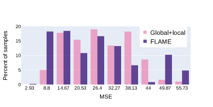
Figure 6: Histogram of MSE for shape fitting on occluded face images by FLAME [22] and our Global+local model.

Occlusion	FLAME+DPP			Global+Local+DPP			Gloal+Local+VAE			Diverse3DFace (Ours)
Type	ASD-V $(\downarrow)$	ASD-O $(\uparrow)$	$\mathbf{\frac{ASD-O}{ASD-V}}(\uparrow)$	ASD-V $(\downarrow)$	ASD-O $(\uparrow)$	$\mathbf{\frac{ASD-O}{ASD-V}}(\uparrow)$	ASD-V $(\downarrow)$	ASD-O $(\uparrow)$	$\mathbf{\frac{ASD-O}{ASD-V}}(\uparrow)$	ASD-V $(\downarrow)$	ASD-O $(\uparrow)$	$\frac{ASD-O}{ASD-V}(\uparrow)$
Glasses	3.44	2.98	0.866	2.15	2.99	1.391	0.81	1.17	1.444	0.68	3.56	5.235
Face-mask	3.45	4.93	1.429	2.85	3.99	1.400	0.75	1.62	2.160	1.03	7.47	7.252
Random	4.12	4.23	1.027	3.17	3.84	1.211	0.79	1.29	1.633	0.83	4.30	5.181
Overall	3.86	4.44	1.150	3.03	3.88	1.281	0.78	1.41	1.808	0.90	5.41	6.011

Table 3: Quantitative evaluation of the diversity in 3D reconstruction of occluded faces from the CelebA dataset [23] between the baselines vs. Diverse3DFace in terms of the ASD-V and ASD-O metrics (in order of $10^{-3}$) and the ratio between them.

	1	2	3	4	5
0.1	0.53	0.81	0.93	1.40	1.88
0.25	0.69	0.95	1.18	1.61	1.98
0.5	0.86	1.02	1.30	1.94	2.14
1	0.81	1.05	1.23	1.92	2.03
2	0.79	0.98	1.06	1.57	1.98

(a) ASD-V $(\downarrow)$

	1	2	3	4	5
0.1	3.63	4.92	5.62	7.17	8.64
0.25	4.13	6.37	7.65	8.18	10.73
0.5	5.98	8.25	9.16	11.19	14.53
1	5.18	7.89	8.84	10.72	12.96
2	4.42	6.68	7.40	9.78	12.21

(b) ASD-O $(\uparrow)$

Table 4: Effect of the hyperparameters $k$ and $n_{\sigma}$ on the diversity metrics ASD-V and ASD-O on the CoMA dataset [31].

Figure 7: Set of 3D reconstructions by Diverse3DFace on real-world occluded face images.

Figure 8: Qualitative evaluation of the diversity and robustness performance of Diverse3DFace to occlusions at different facial locations.

Figure 9: Controlled generated of diverse 3D reconstructions between two distinct modes. Diverse3DFace can be used to generate controlled diversity on the occluded regions by performing interpolation between two distinct shapes in the latent space.

Figure 10: More Qualitative evaluation on the CelebA dataset [23]: Reconstructed singular 3D meshes from the target image by the baselines vs. the diverse reconstructions from Diverse3DFace.

A.1 Further Quantitative Analysis on Diversity

We provide further quantitative evaluation of our approach compared to the baselines in terms of diversity performance as measured by the proposed ASD-O, ASD-V metrics, and the ratio ASD-O/ASD-V, on the CelebA dataset [23]. Since the CelebA dataset [23] is not labeled with groundtruth 3D shape, we do not compute the Closest Sample Distance (CES) on this dataset. To re-iterate, lower ASD-V indicates better consistency with the visible regions; and higher ASD-O indicates higher diversity in the occluded regions. As reported in  Tab. 3, our approach obtains the maximum ASD-O across all occlusion types, the lowest ASD-V for Glasses, as well as the second lowest (compared to Mesh-VAE) ASD-V for Facemasks and Random occlusions. This is further corroborated by the significantly higher ASD-O/ASD-V ratios reported by Diverse3DFace compared to the baselines. Compared to this, single-stage diversity fitting baselines viz. FLAME+DPP and Global+Local+DPP generate the lowest ASD-O/ASD-V ratios, signifying that the 3D reconstructions generated by these approaches are neither diverse on the occluded regions, nor consistent with respect to the visible regions. On the other hand, one-pass samples generated by Global+Local+VAE are consistent with the visible face as reported by low ASD-V, but not diverse on the occluded regions (low ASD-O).

A.2 Error Histogram Analysis

In  Fig. 6, we plot the histograms of shape fitting errors (in terms of MSE) when the FLAME [22] and our global+local model are used to fit to partially occluded face images. One can observe that, while FLAME registers smaller errors (less than 10 MSE) on more number of samples than the global+local model, there are significantly more number of samples $(\sim 15\%)$ where FLAME registers very high MSE errors ($>50$ MSE) than the global+local model. One can conclude that our global+local model is more robust than the global FLAME model [22] on samples with challenging occlusions.

A.3 Diversity Hyperparameters

The diversity generated by our approach is determined by the DPP loss $L_{dpp}=-tr\left(\mathbf{I}-(\mathbf{L}+\mathbf{I})^{-1}\right)$. Here, the DPP kernel entry for the $i,j$-th element is given by $L_{i,j}=q_{i}S_{i,j}q_{j}$, where $q_{i}$ denotes the quality of element $i$, and $S_{i,j}$ represents the similarity between $i$ and $j$. The DPP optimization tries to maximize the quality of each sample, while minimizing the similarity between distinct samples. As stated in the main paper, we control the similarity term $S_{i,j}=\exp\left(-\frac{k}{\operatorname{median}_{i,j}(dist_{i,j})}dist_{i,j}\right)$ and the quality term $q_{i}=\exp(-\max(0,\mathbf{z}_{i}^{T}\mathbf{z}_{i}-n_{\sigma}\sqrt{d}))$ using two parameters $k$ and $n_{\sigma}$, respectively. In  Tab. 4, we study the effects of the two hyper-parameters $k$ and $n_{\sigma}$ on diversity as measured by the diversity metrics ASD-V and ASD-O. As shown in  Tab. 4, we obtain maximum ASD-V, as well as, ASD-O at $k=0.5$; whereas both metrics increase as $n_{\sigma}$ increases. Thus, we set $k=0.5$ in our experiments while we choose $n_{\sigma}=3$ as a sweet spot between minimizing ASD-V and maximizing ASD-O. The user can change the value of $n_{\sigma}$ to tweak the diversity-realism trade-off.

A.4 Real-world Occlusions

We present examples of diverse 3D reconstructions by our approach on real-world occluded face images in  Fig. 7. For these images, we inferred the occlusion mask using the face segmentation model by Nirkin et al. [27]. These results further demonstrate the efficacy of Diverse3DFace to generate diverse, yet plausible 3D reconstructions on real world occlusions ranging from glasses, scarf, facemasks, etc.

A.5 Moving the Occlusion Around the Face

In this section, we evaluate the diversity and robustness performance of Diverse3DFace to occlusions at different locations on the face.  Fig. 8 shows the set of 3D reconstruction by Diverse3DFace when the occlusion moves around the face occupying the left cheek, mouth, the right cheek, center and the periocular (eye) regions of the face. Our method generates diverse, yet plausible set of 3D reconstructions for all the cases. We particularly note the high degree of diversity in expression that occurs when the mouth region is occluded, as is expected.

A.6 Diversity Interpolations

A potential application of Diverse3DFace is to perform controlled diversification around an occluded region during 3D reconstruction. To do this, we can first generate a set of diverse 3D reconstructions for an occluded target image and then allow the user to select two distinct samples to perform interpolation in-between. We perform interpolation in the latent space: $\mathbf{z}(\alpha)=\alpha\mathbf{z}_{1}+(1-\alpha)\mathbf{z}_{2}$. This affords the user control over the extent and type of diversity. We present examples of such interpolations in  Fig. 9.

A.7 Further Qualitative Results on CelebA Dataset

We show further qualitative results of diverse 3D reconstructions on occluded face images from the CelebA dataset [23] by Diverse3DFace, compared to the singular reconstruction by FLAME [22], DECA [12], CFR-GAN [18], Occ3DMM [9] and Extreme3D [44] in  Fig. 10. While the baselines often get the pose, shape or expression wrong, Diverse3DFace generates 3D reconstructions that are consistent with the visible regions, yet plausibly diverse on the occluded regions.

Appendix B Implementation Details

B.1 Optimization

We use the PyTorch library to implement our approach. In our experiments, we found that the SGD optimizer, with a learning rate of $5\times 10^{-3}$ gives the best results as compared to the Adam and RMSprop optimizers. For photometric fitting, we used the texture model provided by FLAME. We run the fitting stage (Algorithm 1) for $n_{iter}=2000$ iterations and the diversity stage (Algorithm 2) for $n_{comp}=300$ iterations. In Algorithm 1, we set the loss weights as follows: $\lambda_{1}^{f}=5,\lambda_{2}^{f}=16,\lambda_{3}^{f}=10^{-3}$. During the diversifying shape completion stage (Algorithm 2), we set $\lambda_{1}=1000,\lambda_{2}=500,\lambda_{3}=0.025$. Further, we found that using a slightly smaller learning rate for the eyeball components while fitting the global+local model gives better results. For these components, we set the learning rate to be 0.5 times that of the other components.

B.2 Mesh-VAE

The Mesh-VAE model is based on the fully convolutional mesh autoencoder (Meshconv) architecture proposed by Zhou et al. [54]. Meshconv [54] uses spatially varying convolutional kernels for different mesh vertices to account for the irregular structure of a 3D mesh. The spatially varying kernels are sampled from the span of a shared weight basis, using learned per-vertex coefficients. In addition, Meshconv defines pooling and unpooling operations on a 3D mesh by performing feature aggregation Monte Carlo sampling [54].

We trained the Mesh-VAE with FLAME [22] registered groundtruth scans provided in the CoMA [31] and D3DFACS [7] datasets. We perturbed the input meshes with uniformly sampled rectangular masks (in XY) within a range around the mesh center, while gradually increasing the size of the mask per training epoch until it covered $\sim$40% of the vertices. We detail the network architecture for the Mesh-VAE in  Tabs. 5 and 6.

The abbreviated operators used are defined as follows:

• vcDownConv($in_{c},out_{c},s,r,M$) + vcDownRes($s$): Downward residual block (as defined in Meshconv [54]), with $in_{c}$ input channels, $out_{c}$ output channels, $s$ stride, $r$ kernel radius and $M$ number of shared weight bases. The output is activated with ELU [6] activation.

• vcUpConv($in_{c},out_{c},s,r,M$) + vcUpRes($s$): Upward residual block (as defined in Meshconv [54]), with $in_{c}$ input channels, $out_{c}$ output channels, $s$ stride, $r$ kernel radius and $M$ number of shared weight bases. The output is activated with ELU [6] activation.

Table 5: Network architecture of the Mesh-VAE Encoder $\mathcal{E}_{mesh}$.

Input	Layer	Output size	Output
$5023\times 3$ Mesh	$\rightarrow$ vcDownConv($in_{c}=3,out_{c}=32,s=2,r=43,M=17$) + vcDownRes(2)	$1367\times 32$
	vcDownConv($in_{c}=32,out_{c}=64,s=1,r=27,M=17$) + vcDownRes(1)	$1367\times 64$
	vcDownConv($in_{c}=64,out_{c}=128,s=2,r=54,M=17$) + vcDownRes(2)	$270\times 128$
	vcDownConv($in_{c}=128,out_{c}=256,s=1,r=25,M=17$) + vcDownRes(1)	$270\times 256$
	vcDownConv($in_{c}=256,out_{c}=512,s=2,r=81,M=17$) + vcDownRes(2)	$45\times 512$
	vcDownConv($in_{c}=512,out_{c}=1024,s=1,r=27,M=17$) + vcDownRes(1)	$45\times 1024$	feats
feats	vcDownConv($in_{c}=1024,out_{c}=64,s=2,r=37,M=17$) + vcDownRes(2)	$10\times 64$	$\bm{\mu}$
feats	vcDownConv($in_{c}=1024,out_{c}=64,s=2,r=37,M=17$) + vcDownRes(2)	$10\times 64$	$\log\bm{\sigma}^{2}$
Model Complexity	9M

Table 6: Network architecture of the Mesh-VAE Decoder $\mathcal{D}_{mesh}$.

Input	Layer	Output size	Output
$10\times 64$ $\mathbf{z}$	vcUpConv($in_{c}=64,out_{c}=1024,s=2,r=8,M=17$) + vcUpRes(2)	$45\times 1024$
	vcUpConv($in_{c}=1024,out_{c}=512,s=1,r=27,M=17$) + vcUpRes(1)	$45\times 512$
	vcUpConv($in_{c}=512,out_{c}=256,s=2,r=16,M=17$) + vcUpRes(2)	$270\times 256$
	vcUpConv($in_{c}=256,out_{c}=128,s=1,r=25,M=17$) + vcUpRes(1)	$270\times 128$
	vcUpConv($in_{c}=128,out_{c}=64,s=2,r=12,M=17$) + vcUpRes(2)	$1367\times 64$
	vcUpConv($in_{c}=64,out_{c}=32,s=1,r=27,M=17$) + vcUpRes(1)	$1367\times 32$
	vcUpConv($in_{c}=32,out_{c}=3,s=2,r=24,M=17$) + vcUpRes(2)	$5023\times 3$	Output
Model Complexity	8M

References

- [1] Yuval Bahat and Tomer Michaeli. Explorable super resolution. In Proceedings of the IEEE/CVF Conference on Computer Vision and Pattern Recognition, pages 2716–2725, 2020.
- [2] Yoshua Bengio, Jérôme Louradour, Ronan Collobert, and Jason Weston. Curriculum learning. In International Conference on Machine Learning, 2009.
- [3] Volker Blanz and Thomas Vetter. A morphable model for the synthesis of 3d faces. In Proceedings of the 26th annual conference on Computer graphics and interactive techniques, pages 187–194, 1999.
- [4] Giorgos Bouritsas, Sergiy Bokhnyak, Stylianos Ploumpis, Michael Bronstein, and Stefanos Zafeiriou. Neural 3d morphable models: Spiral convolutional networks for 3d shape representation learning and generation. In Proceedings of the IEEE/CVF International Conference on Computer Vision, pages 7213–7222, 2019.
- [5] Tong Che, Yanran Li, Athul Paul Jacob, Yoshua Bengio, and Wenjie Li. Mode regularized generative adversarial networks. arXiv preprint arXiv:1612.02136, 2016.
- [6] Djork-Arné Clevert, Thomas Unterthiner, and Sepp Hochreiter. Fast and accurate deep network learning by exponential linear units (elus). arXiv preprint arXiv:1511.07289, 2015.
- [7] Darren Cosker, Eva Krumhuber, and Adrian Hilton. A facs valid 3d dynamic action unit database with applications to 3d dynamic morphable facial modeling. In 2011 international conference on computer vision, pages 2296–2303. IEEE, 2011.
- [8] Michaël Defferrard, Xavier Bresson, and Pierre Vandergheynst. Convolutional neural networks on graphs with fast localized spectral filtering. Advances in neural information processing systems, 29:3844–3852, 2016.
- [9] Bernhard Egger, Sandro Schönborn, Andreas Schneider, Adam Kortylewski, Andreas Morel-Forster, Clemens Blumer, and Thomas Vetter. Occlusion-aware 3d morphable models and an illumination prior for face image analysis. International Journal of Computer Vision, 126(12):1269–1287, 2018.
- [10] Bernhard Egger, William AP Smith, Ayush Tewari, Stefanie Wuhrer, Michael Zollhoefer, Thabo Beeler, Florian Bernard, Timo Bolkart, Adam Kortylewski, Sami Romdhani, et al. 3d morphable face models—past, present, and future. ACM Transactions on Graphics (TOG), 39(5):1–38, 2020.
- [11] Mohamed Elfeki, Camille Couprie, Morgane Riviere, and Mohamed Elhoseiny. Gdpp: Learning diverse generations using determinantal point processes. In International Conference on Machine Learning, pages 1774–1783. PMLR, 2019.
- [12] Yao Feng, Haiwen Feng, Michael J Black, and Timo Bolkart. Learning an animatable detailed 3d face model from in-the-wild images. ACM Transactions on Graphics (TOG), 40(4):1–13, 2021.
- [13] Baris Gecer, Stylianos Ploumpis, Irene Kotsia, and Stefanos Zafeiriou. Ganfit: Generative adversarial network fitting for high fidelity 3d face reconstruction. In Proceedings of the IEEE/CVF Conference on Computer Vision and Pattern Recognition (CVPR), June 2019.
- [14] Thomas Gerig, Andreas Morel-Forster, Clemens Blumer, Bernhard Egger, Marcel Luthi, Sandro Schönborn, and Thomas Vetter. Morphable face models-an open framework. In 2018 13th IEEE International Conference on Automatic Face & Gesture Recognition (FG 2018), pages 75–82. IEEE, 2018.
- [15] Arnab Ghosh, Viveka Kulharia, Vinay P. Namboodiri, Philip H.S. Torr, and Puneet K. Dokania. Multi-agent diverse generative adversarial networks. In Proceedings of the IEEE Conference on Computer Vision and Pattern Recognition (CVPR), June 2018.
- [16] Ian Goodfellow, Jean Pouget-Abadie, Mehdi Mirza, Bing Xu, David Warde-Farley, Sherjil Ozair, Aaron Courville, and Yoshua Bengio. Generative adversarial nets. In Advances in neural information processing systems, pages 2672–2680, 2014.
- [17] Phillip Isola, Jun-Yan Zhu, Tinghui Zhou, and Alexei A Efros. Image-to-image translation with conditional adversarial networks. In Proceedings of the IEEE conference on computer vision and pattern recognition, pages 1125–1134, 2017.
- [18] Yeong-Joon Ju, Gun-Hee Lee, Jung-Ho Hong, and Seong-Whan Lee. Complete face recovery gan: Unsupervised joint face rotation and de-occlusion from a single-view image. In WACV, 2022.
- [19] Hyeongwoo Kim, Michael Zollhöfer, Ayush Tewari, Justus Thies, Christian Richardt, and Christian Theobalt. Inversefacenet: Deep monocular inverse face rendering. In Proceedings of the IEEE Conference on Computer Vision and Pattern Recognition, pages 4625–4634, 2018.
- [20] Thomas N Kipf and Max Welling. Semi-supervised classification with graph convolutional networks. arXiv preprint arXiv:1609.02907, 2016.
- [21] Alex Kulesza and Ben Taskar. Determinantal point processes for machine learning. arXiv preprint arXiv:1207.6083, 2012.
- [22] Tianye Li, Timo Bolkart, Michael. J. Black, Hao Li, and Javier Romero. Learning a model of facial shape and expression from 4D scans. ACM Transactions on Graphics, (Proc. SIGGRAPH Asia), 36(6):194:1–194:17, 2017.
- [23] Ziwei Liu, Ping Luo, Xiaogang Wang, and Xiaoou Tang. Deep learning face attributes in the wild. In Proceedings of International Conference on Computer Vision (ICCV), December 2015.
- [24] Odile Macchi. The coincidence approach to stochastic point processes. Advances in Applied Probability, 7(1):83–122, 1975.
- [25] Christopher Morris, Martin Ritzert, Matthias Fey, William L Hamilton, Jan Eric Lenssen, Gaurav Rattan, and Martin Grohe. Weisfeiler and leman go neural: Higher-order graph neural networks. In Proceedings of the AAAI Conference on Artificial Intelligence, volume 33, pages 4602–4609, 2019.
- [26] Thomas Neumann, Kiran Varanasi, Stephan Wenger, Markus Wacker, Marcus Magnor, and Christian Theobalt. Sparse localized deformation components. ACM Transactions on Graphics (TOG), 32(6):1–10, 2013.
- [27] Yuval Nirkin, Iacopo Masi, Anh Tran Tuan, Tal Hassner, and Gerard Medioni. On face segmentation, face swapping, and face perception. In 2018 13th IEEE International Conference on Automatic Face & Gesture Recognition (FG 2018), pages 98–105. IEEE, 2018.
- [28] Pascal Paysan, Reinhard Knothe, Brian Amberg, Sami Romdhani, and Thomas Vetter. A 3d face model for pose and illumination invariant face recognition. In 2009 Sixth IEEE International Conference on Advanced Video and Signal Based Surveillance, pages 296–301. Ieee, 2009.
- [29] Stylianos Ploumpis, Evangelos Ververas, Eimear O’Sullivan, Stylianos Moschoglou, Haoyang Wang, Nick Pears, William Smith, Baris Gecer, and Stefanos P Zafeiriou. Towards a complete 3d morphable model of the human head. IEEE Transactions on Pattern Analysis and Machine Intelligence, 2020.
- [30] Eduard Ramon, Gil Triginer, Janna Escur, Albert Pumarola, Jaime Garcia, Xavier Giro-i Nieto, and Francesc Moreno-Noguer. H3d-net: Few-shot high-fidelity 3d head reconstruction. In Proceedings of the IEEE/CVF International Conference on Computer Vision, pages 5620–5629, 2021.
- [31] Anurag Ranjan, Timo Bolkart, Soubhik Sanyal, and Michael J. Black. Generating 3D faces using convolutional mesh autoencoders. In European Conference on Computer Vision (ECCV), pages 725–741, 2018.
- [32] Shunsuke Saito, Tianye Li, and Hao Li. Real-time facial segmentation and performance capture from rgb input. In European conference on computer vision, pages 244–261. Springer, 2016.
- [33] Soubhik Sanyal, Timo Bolkart, Haiwen Feng, and Michael J Black. Learning to regress 3d face shape and expression from an image without 3d supervision. In Proceedings of the IEEE/CVF Conference on Computer Vision and Pattern Recognition, pages 7763–7772, 2019.
- [34] Gabriel Schwartz, Shih-En Wei, Te-Li Wang, Stephen Lombardi, Tomas Simon, Jason Saragih, and Yaser Sheikh. The eyes have it: An integrated eye and face model for photorealistic facial animation. ACM Trans. Graph., 39(4), jul 2020.
- [35] Soumyadip Sengupta, Angjoo Kanazawa, Carlos D Castillo, and David W Jacobs. Sfsnet: Learning shape, reflectance and illuminance of facesin the wild’. In Proceedings of the IEEE Conference on Computer Vision and Pattern Recognition, pages 6296–6305, 2018.
- [36] Zhixin Shu, Ersin Yumer, Sunil Hadap, Kalyan Sunkavalli, Eli Shechtman, and Dimitris Samaras. Neural face editing with intrinsic image disentangling. In Proceedings of the IEEE conference on computer vision and pattern recognition, pages 5541–5550, 2017.
- [37] Kihyuk Sohn, Honglak Lee, and Xinchen Yan. Learning structured output representation using deep conditional generative models. Advances in neural information processing systems, 28:3483–3491, 2015.
- [38] Akash Srivastava, Lazar Valkov, Chris Russell, Michael U Gutmann, and Charles Sutton. Veegan: Reducing mode collapse in gans using implicit variational learning. In Proceedings of the 31st International Conference on Neural Information Processing Systems, pages 3310–3320, 2017.
- [39] Masahiro Suzuki, Kotaro Nakayama, and Yutaka Matsuo. Joint multimodal learning with deep generative models. arXiv preprint arXiv:1611.01891, 2016.
- [40] Ayush Tewari, Michael Zollhofer, Hyeongwoo Kim, Pablo Garrido, Florian Bernard, Patrick Perez, and Christian Theobalt. Mofa: Model-based deep convolutional face autoencoder for unsupervised monocular reconstruction. In Proceedings of the IEEE International Conference on Computer Vision Workshops, pages 1274–1283, 2017.
- [41] Luan Tran, Feng Liu, and Xiaoming Liu. Towards high-fidelity nonlinear 3d face morphable model. In Proceedings of the IEEE Conference on Computer Vision and Pattern Recognition, pages 1126–1135, 2019.
- [42] Luan Tran and Xiaoming Liu. On learning 3d face morphable model from in-the-wild images. IEEE transactions on pattern analysis and machine intelligence, 2019.
- [43] Anh Tuan Tran, Tal Hassner, Iacopo Masi, and Gérard Medioni. Regressing robust and discriminative 3d morphable models with a very deep neural network. In Proceedings of the IEEE conference on computer vision and pattern recognition, pages 5163–5172, 2017.
- [44] Anh Tuán Trán, Tal Hassner, Iacopo Masi, Eran Paz, Yuval Nirkin, and Gérard Medioni. Extreme 3d face reconstruction: Seeing through occlusions. In Proceedings of the IEEE Conference on Computer Vision and Pattern Recognition, pages 3935–3944, 2018.
- [45] Petar Veličković, Guillem Cucurull, Arantxa Casanova, Adriana Romero, Pietro Lio, and Yoshua Bengio. Graph attention networks. arXiv preprint arXiv:1710.10903, 2017.
- [46] Jingdong Wang, Ke Sun, Tianheng Cheng, Borui Jiang, Chaorui Deng, Yang Zhao, Dong Liu, Yadong Mu, Mingkui Tan, Xinggang Wang, et al. Deep high-resolution representation learning for visual recognition. IEEE transactions on pattern analysis and machine intelligence, 2020.
- [47] Huawei Wei, Shuang Liang, and Yichen Wei. 3d dense face alignment via graph convolution networks. arXiv preprint arXiv:1904.05562, 2019.
- [48] Shangzhe Wu, Christian Rupprecht, and Andrea Vedaldi. Unsupervised learning of probably symmetric deformable 3d objects from images in the wild. In Proceedings of the IEEE/CVF Conference on Computer Vision and Pattern Recognition, pages 1–10, 2020.
- [49] Dingdong Yang, Seunghoon Hong, Yunseok Jang, Tianchen Zhao, and Honglak Lee. Diversity-sensitive conditional generative adversarial networks. arXiv preprint arXiv:1901.09024, 2019.
- [50] Tarun Yenamandra, Ayush Tewari, Florian Bernard, Hans-Peter Seidel, Mohamed Elgharib, Daniel Cremers, and Christian Theobalt. i3dmm: Deep implicit 3d morphable model of human heads. In Proceedings of the IEEE/CVF Conference on Computer Vision and Pattern Recognition, pages 12803–12813, 2021.
- [51] Ye Yuan and Kris Kitani. Diverse trajectory forecasting with determinantal point processes. arXiv preprint arXiv:1907.04967, 2019.
- [52] Ye Yuan and Kris Kitani. Dlow: Diversifying latent flows for diverse human motion prediction. In European Conference on Computer Vision, pages 346–364. Springer, 2020.
- [53] Chuanxia Zheng, Tat-Jen Cham, and Jianfei Cai. Pluralistic image completion. In Proceedings of the IEEE/CVF Conference on Computer Vision and Pattern Recognition, pages 1438–1447, 2019.
- [54] Yi Zhou, Chenglei Wu, Zimo Li, Chen Cao, Yuting Ye, Jason Saragih, Hao Li, and Yaser Sheikh. Fully convolutional mesh autoencoder using efficient spatially varying kernels. arXiv preprint arXiv:2006.04325, 2020.
- [55] Jun-Yan Zhu, Richard Zhang, Deepak Pathak, Trevor Darrell, Alexei A Efros, Oliver Wang, and Eli Shechtman. Multimodal image-to-image translation by enforcing bi-cycle consistency. In Advances in neural information processing systems, pages 465–476, 2017.
- [56] Michael Zollhöfer, Justus Thies, Pablo Garrido, Derek Bradley, Thabo Beeler, Patrick Pérez, Marc Stamminger, Matthias Nießner, and Christian Theobalt. State of the art on monocular 3d face reconstruction, tracking, and applications. In Computer Graphics Forum, volume 37, pages 523–550. Wiley Online Library, 2018.