A fast method for evaluating Volume potentials in the Galerkin boundary element method

Abstract

Three algorithm are proposed to evaluate volume potentials that arise in boundary element methods for elliptic PDEs. The approach is to apply a modified fast multipole method for a boundary concentrated volume mesh. If $h$ is the meshwidth of the boundary, then the volume is discretized using nearly $\mathcal{O}(h^{-2})$ degrees of freedom, and the algorithm computes potentials in nearly $\mathcal{O}(h^{-2})$ complexity. Here nearly means that logarithmic terms of $h$ may appear. Thus the complexity of volume potentials calculations is of the same asymptotic order as boundary potentials. For sources and potentials with sufficient regularity the parameters of the algorithm can be designed such that the error of the approximated potential converges at any specified rate $\mathcal{O}(h^{p})$. The accuracy and effectiveness of the proposed algorithms are demonstrated for potentials of the Poisson equation in three dimensions.

65N38, 65N12, 65N30

1 Introduction

Boundary integral methods for homogeneous elliptic partial differential equations are based on representing the solution in form of layer potentials. This results in an integral equation on the boundary of the domain. For a three dimensional domain this implies a reduction to a problem on the two dimensional boundary. After discretization with a boundary mesh of size $h$, one obtains a dense matrix of size $O(h^{-2})$. Typically, the linear system is solved iteratively, where the dominant numerical cost is the evaluation of matrix-vector products. There are several well established methods to accelerate this operation. This includes the fast multipole method [7, 17, 22], wavelets [5] and $\mathcal{H}$-matrix algebra [4] which can be combined with adaptive cross approximation [3]. With these methods it is possible to approximately compute the matrix-vector product with nearly or even exactly $O(h^{-2})$ complexity, while maintaining the convergence rate of the discretization error.

If the underlying PDE is inhomogeneous, the solution must be represented with an additional volume potential of the right hand side of the equation. Likewise, the reconstruction of the solution in the domain requires the evaluation of layer potentials in the volume. The efficient evaluation volume potentials has been the subject of many investigations. A popular method is the dual reciprocity method. Here the basic idea is to approximate the right hand side by radial basis functions, and to use integration by parts to convert the volume integral to a boundary integral, see, e.g., [19]. The approach in [6] is based on related ideas. Another frequently used approach is to embed the domain into a rectangular box and apply either the fast multipole method [14, 1] or a fast Poisson solver in the box. To avoid difficulties extending the right hand side beyond the domain one can discretize the volume, for instance, with a tetrahedral mesh and use a fast method for the evaluation of the domain integral, see [18].

We also mention some methods for two dimensional domains that either rely on a Fourier-Galerkin discretization of the boundary curve [8] or are specific to circular domains [2, 21]. A comparison of different domain evaluation techniques is given in [10].

However, the order of the complexity will be increased when volume potentials appear in the integral equation. Likewise, the evaluation of the solution will increase the complexity if a uniform volume mesh is used for the domain evaluations of layer or volume potentials. We will therefore consider discretizations using a boundary concentrated (BC) mesh, where the meshwidth of the volume discretization grows proportionally with the distance from the boundary. This kind of mesh has already been employed in the context of finite element methods [12]. The number elements in such a mesh is order $O(h^{-2})$ where $h$ is the meshwidth of the boundary mesh. Hence the number of elements of in the boundary and volume meshes have the same asymptotic order. In this article, we will derive fast algorithms for the following computational tasks.

• Volume to volume (VtV). Given a function represented by the BC mesh, compute its volume potential on the BC mesh.

• Volume to boundary (VtB). Given a function represented by the BC mesh, compute the volume potential on the surface mesh.

• Boundary to volume (BtV). Given a density represented by the surface mesh, compute its layer potential on the BC mesh.

In particular, we will devise a fast multipole algorithm for BC meshes and show that its parameters can be chosen such that it has nearly optimal $O(h^{-2})$ complexity.

This paper is organized as follows. In the remainder of this section we provide more detailed background material on layer and volume integrals and their discretization. A hierarchical subdivision of the volume by a boundary concentrated meshes is then described in section 2. Section 3 describes a fast multipole type algorithm to efficiently perform the VtV, VtB and BtV calculations. Section 4 provides an analysis of the complexity and accuracy of the methods. We conclude in section 5 with numerical results that illustrate the theoretical results.

1.1 Boundary and Volume Potentials

Consider an elliptic operator $\mathcal{L}$ with constant coefficients in a bounded domain $\Omega\subset\mathbb{R}^{3}$ with boundary surface $\Gamma=\partial\Omega$. The Green’s representation formula expresses the solution of $\mathcal{L}u=f$ in $\Omega$ in terms of the Dirichlet and Neumann data on $\Gamma$

(1) $$u=\tilde{\mathcal{V}}[\gamma_{1}u]-\tilde{\mathcal{K}}[\gamma_{0}u]+\tilde{\mathcal{N}}f,\qquad\text{in}\;\Omega.$$

Here, $\gamma_{0}u$ and $\gamma_{1}u$ are the boundary trace and normal boundary trace of a function $u$ defined in the domain, and $\tilde{\mathcal{V}}$ and $\tilde{\mathcal{K}}$ are the single-layer and double-layer potentials, defined by

$$\tilde{\mathcal{V}}q(\mathbf{x}) =\int_{\Gamma}G(\mathbf{x},\mathbf{y})q(\mathbf{y})\,ds_{\mathbf{y}}\,,$$

$$\tilde{\mathcal{K}}u(\mathbf{x}) =\int_{\Gamma}\frac{\partial G}{\partial n_{\mathbf{y}}}(\mathbf{x},\mathbf{y})u(\mathbf{y})\,ds_{\mathbf{y}}.$$

Moreover, $\tilde{\mathcal{N}}$ denotes the volume (or sometimes Newton) potential

$$\tilde{\mathcal{N}}f(\mathbf{x})=\int_{\Omega}G(\mathbf{x},\mathbf{y})f(\mathbf{y})\,d\mathbf{y}.$$

The kernel $G(\cdot,\cdot)$ is the free space Green’s function of the PDE, which in the case of the Poisson equation is

$$G(\mathbf{x},\mathbf{y})=\frac{1}{4\pi}\frac{1}{\left|\mathbf{x}-\mathbf{y}\right|}.$$

Taking the boundary trace in (1) results in the Green’s integral equation

(2) $$\frac{1}{2}\gamma_{0}u=\mathcal{V}[\gamma_{1}u]-\mathcal{K}[\gamma_{0}u]+\mathcal{N}f,\qquad\text{on}\;\Gamma.$$

In (1) the operators with a tilde indicate that a potential is evaluated in the domain, and in (2) the potentials without the tilde indicates the evaluation on the boundary. It is well known that the potentials are continuous in the following spaces

$$\tilde{\mathcal{V}}:H^{-\frac{1}{2}}(\Gamma)\to H^{1}(\Omega), \quad\mathcal{V}:H^{-\frac{1}{2}}(\Gamma)\to H^{\frac{1}{2}}(\Gamma),$$

$$\tilde{\mathcal{K}}:H^{\frac{1}{2}}(\Gamma)\to H^{1}(\Omega), \quad\mathcal{K}:H^{\frac{1}{2}}(\Gamma)\to H^{\frac{1}{2}}(\Gamma),$$

$$\tilde{\mathcal{N}}:H^{-1}(\Omega)\to H^{1}(\Omega), \quad\mathcal{N}:H^{-1}(\Omega)\to H^{\frac{1}{2}}(\Gamma),$$

see, e.g., [9, 15]. In the direct boundary element method, the integral equation (2) is solved for the missing boundary data, and then the solution in the interior is evaluated using the Green’s representation formula.

1.2 Discretization

We briefly describe the Galerkin discretization of surface and volume integral operators. To fix ideas, assume that $\Omega$ is a polyhedral domain that has been subdivided into a tetrahedral mesh $\mathcal{T}$. We assume that this volume mesh is shape regular, but not necessarily conforming or quasi-uniform. However, we assume that the restriction to the boundary is a conforming, shape regular, and quasi-uniform triangular mesh of meshwidth $h$. The boundary mesh is denoted by $\mathcal{S}$.

Suppose we want to solve the Dirichlet problem using the direct integral formulation. In this case the Green’s integral formulation (2) is solved for the Neumann data, and then the representation formula (1) provides the solution in the domain.

The Galerkin discretization of the integral equation is based on the finite element space $S^{\Gamma}_{h}$. A typical choice for $S^{\Gamma}_{h}$ are low-order piecewise polynomial functions on $\mathcal{S}$. The Galerkin discretization of (2) reads: find $q_{h}\in S_{h}^{\Gamma}$ such that

(3) $$\left\langle\varphi,\mathcal{V}q_{h}\right\rangle_{L_{2}(\Gamma)}=\left\langle\varphi,\left(1/2+\mathcal{K}\right)g\right\rangle_{L_{2}(\Gamma)}-\left\langle\varphi,\mathcal{N}f\right\rangle_{L_{2}(\Gamma)}$$

for all basis functions $\varphi$ of $S^{\Gamma}_{h}$. Here $\left\langle\cdot,\cdot\right\rangle_{L_{2}(\Gamma)}$ is the $L_{2}$-inner product on $\Gamma$, $q_{h}$ is the approximation of the Neumann data and $g$ is the given Dirichlet data. Since $q_{h}$ and is a linear combination of all $\varphi$’s this leads to a linear system

$$V\mathbf{q}=\mathbf{b},$$

where $\mathbf{q}$ is the vector of coefficients in the expansion of $q_{h}$ in the basis, and the coefficients of $\mathbf{b}$ are given by the right hand side in (3).

For the approximation of the solution in the volume we also use a variational approach. To that end, the potential $u$ is approximated in the space of piecewise polynomial functions $S^{\Omega}_{h}$ on $\mathcal{T}$. Since in BC meshes the size of the elements varies, the polynomial order $p_{\omega}$ is tied to the size of the elements. The precise relationship will be discussed in section 4 below.

For a tetrahedron orthogonal polynomials $\phi^{\alpha}_{\omega},\left|\alpha\right|\leq p_{\omega}$ can be constructed explicitly in terms of Jacobi polynomials, see [13]. Outside of $\omega$ these functions are extended by zero. Thus the finite element space is

(4) $$S^{\Omega}_{h}=\mbox{span}\left\{\phi^{\alpha}_{\omega}\;:\;\omega\in\mathcal{T},\;\left|\alpha\right|\leq p_{\omega}\right\}.$$

The space $S^{\Omega}_{h}$ is a subset of $L_{2}(\Omega)$, but it is not contained in $H^{1}(\Omega)$. However, this is sufficient regularity for the $L_{2}(\Omega)$-orthogonal projection which is given as follows,

(5) $$P_{\mathcal{T}}u =\sum_{\omega\in\mathcal{T}}\sum_{\left|\alpha\right|\leq p_{\omega}}u_{\alpha,\omega}{\phi^{\alpha}_{\omega}},$$

where

(6) $$u_{\alpha,\omega} =\left\langle\phi^{\alpha}_{\omega},\tilde{\mathcal{V}}[\gamma_{1}u]-\tilde{\mathcal{K}}[\gamma_{0}u]+\tilde{\mathcal{N}}f\right\rangle_{L_{2}(\Omega)}.$$

In analogy to $S^{\Omega}_{h}$, the space $S^{\Gamma}_{h}$ is spanned by piecewise polynomials on triangles. For the latter all triangles have diameter proportional to $h$ and the polynomial degree $p$ is fixed and typically low. We write

(7) $$S^{\Gamma}_{h}=\mbox{span}\left\{\varphi^{\alpha}_{\gamma}\;:\;\gamma\in\mathcal{S},\;\left|\alpha\right|\leq p\right\}.$$

Here $\alpha$ is a multi index with two components whereas in (4) $\alpha$ has three components.

2 Boundary Concentrated Mesh

This section provides more details for the case that $\mathcal{T}$ is a BC mesh. We consider a polyhedron $\Omega\subset\mathbb{R}^{3}$ that is subdivided into a small number of tetrahedra. These tetrahedra form the coarsest level, or level $\ell=0$ in a hierarchical subdivision of space. The $\ell+1$-st level tetrahedra are obtained by subdividing some or all tetrahedra in the $\ell$-th level into eight tetrahedra. The refinements of a tetrahedron $\omega$ are referred to as the children, or $\mathcal{K}(\omega)$.

Note that some care must be applied to ensure that the refinements remain shape regular, because in general, it is not possible to obtain congruent subdivisions of three dimensional tetrahedra. However, with the refinement scheme introduced in [11] one can limit the number of congruency classes to three which implies shape regularity.

A quasi uniform refinement is achieved if all tetrahedra in a given level are subdivided. In this case a tree structure results, where the children of the root are the tetrahedra of the initial subdivision of $\Omega$. All other nodes either have eight children or are leaves in the finest level. The domain $\Omega$ is the union of all tetrahedra in any given level.

In contrast to uniform refinements, a boundary concentrated refinement is obtained by refining only tetrahedra that are close to the boundary. A two dimensional situation is illustrated in figure 1. The resulting tree structure may have leaves in any level, which are the tetrahedra that have not been refined. The domain $\Omega$ is the union of all leaves in all levels.

Figure 1: A two dimensional illustration of a boundary concentrated refinement.

To describe the BC refinement scheme in detail, denote the center of $\omega$ by $\mathbf{x}_{\omega}$, the diameter by

(8) $$\rho_{\omega}=\max_{{\bf v}:\mbox{\scriptsize vertex of }\omega}\left|{\bf v}-\mathbf{x}_{\omega}\right|.$$

The separation ratio of two tetrahedra in the same level is defined as

(9) $$\eta(\omega,\omega^{\prime})=\frac{\rho_{\omega^{\prime}}+\rho_{\omega^{\prime}}}{\left|\mathbf{x}_{\omega}-\mathbf{x}_{\omega^{\prime}}\right|}\,,\quad\omega\not=\omega^{\prime},$$

and $\eta(\omega,\omega)=\infty$. The neighbors of $\omega$ are the tetrahedra $\omega^{\prime}$ in the same level for which the separation ratio is greater than a predetermined constant $\eta_{0}$. That is,

(10) $$\mathcal{N}(\omega)=\{\omega^{\prime}\in C_{\ell}\,:\,\eta(\omega,\omega^{\prime})>\eta_{0}\}.$$

Here, $C_{\ell}$, denotes the set of all tetrahedra in level $\ell$. Further,

$$B_{\ell}=\{\omega\in C_{\ell}\,:\,\omega\;\text{has a face in}\;\Gamma\}$$

denotes the set of all boundary tetrahedra in level $\ell$. Here it is worth emphasizing that if $\omega$ only has one vertex or one edge in $\Gamma$ it is not included in $B_{\ell}$. Moreover,

$$M_{\ell}=\{\omega\in C_{\ell}\,:\,\mathcal{N}(\omega)\cap B_{\ell}\not=\emptyset\}$$

denotes the tetrahedra that have a boundary tetrahedron among their neighbors. These are the tetrahedra are marked for refinement. Thus

$$L_{\ell}=C_{\ell}\setminus M_{\ell}\,,$$

are the leaves in level $\ell$. The next level list of tetrahedra is

$$C_{\ell+1}=\bigcup\limits_{\omega\in M_{\ell}}\mathcal{K}(\omega).$$

The refinement process is repeated until a finest level $L$ is reached. There, all tetrahedra are leaves, but we distinguish between tetrahedra near the surface and tetrahedra away from the surface. Hence we set $L_{L}=C_{L}\setminus M_{L}$ and denote by $L_{\ell}^{*}$ the set of leaves in any level, i.e.,

$$L_{\ell}^{*}=L_{\ell},\;\ell\in\{0,\dots L-1\}\quad\mbox{and}\quad L_{L}^{*}=C_{L}.$$

We obtain the following subdivision of $\Omega$

(11) $$\mathcal{T}=M_{L}\cup\bigcup\limits_{\ell=0}^{L}L_{\ell}=\bigcup\limits_{\ell=0}^{L}L_{\ell}^{*}\,.$$

An important concept in the fast multipole method is the interaction list $\mathcal{I}(\omega)$, which consists of tetrahedra whose parents are neighbors of the parent of $\omega$, but who are not neighbors with $\omega$ itself. In level zero, we set $\mathcal{I}(\omega)=C_{0}\setminus\mathcal{N}(\omega)$, which can possibly be an empty set.

Since $\mathcal{T}$ is a geometric mesh, it is known that its cardinality is order $4^{L}\sim h^{-2}$, where the constant depends on $\eta_{0}$. It remains to ensure is that the number of neighbors and interacting tetrahedra is bounded.

Theorem 2.1.

The cardinalities $\#\mathcal{N}(\omega)$ and $\#\mathcal{I}(\omega)$ are uniformly bounded. Furthermore, there is a constant $c$ such that

$$\#B_{\ell}\leq c4^{\ell},\quad\#M_{\ell}\leq c4^{\ell},\quad\#L_{\ell}\leq c4^{\ell},\quad\mbox{and }\quad\#C_{\ell}\leq c4^{\ell}.$$

Proof 2.2.

Two tetrahedra $\omega$, $\omega^{\prime}$ in $C_{\ell}$ are neighbors if $\left|\mathbf{x}_{\omega}-\mathbf{x}_{\omega^{\prime}}\right|<(\rho_{\omega}+\rho_{\omega^{\prime}})/\eta_{0}$. If we let $R_{\ell}=\max\{\rho_{\omega}:\omega\in C_{\ell}\}$ then it follows that all neighbors of $\omega$ are contained in the sphere $B_{\omega}$ with center $\mathbf{x}_{\omega}$ and radius $(1+2/\eta_{0})R_{\ell}$.

Further, let $\tilde{\rho}_{\omega}$ be the radius of the largest sphere that is contained in $\omega$, and let $\tilde{R}_{\ell}=\min\{\tilde{\rho}_{\omega}:\omega\in C_{\ell}\}$. Shape regularity implies that $R_{\ell}/\tilde{R}_{\ell}\leq c$. Since the enclosed spheres of the neighbors are contained in $B_{\omega}$ it follows for their volumes that

$$\#\mathcal{N}(\omega)\frac{4\pi}{3}\tilde{R}_{\ell}^{3}\leq\frac{4\pi}{3}\sum_{\omega^{\prime}\in\mathcal{N}(\omega)}\tilde{\rho}_{\omega^{\prime}}^{3}\leq|B_{\omega}|=\frac{4\pi}{3}\left(1+\frac{2}{\eta_{0}}\right)^{3}R_{\ell}^{3},$$

which implies that

$$\#\mathcal{N}(\omega)\leq\frac{R_{\ell}^{3}}{\tilde{R}_{\ell}^{3}}\left(1+\frac{2}{\eta_{0}}\right)^{3}$$

so the number of neighbors is indeed bounded. The boundedness of $\#\mathcal{I}(\omega)$ follows immediately from the definition of interaction lists.

Since all boundary faces are refined into four faces in each step and since each boundary face belongs to only one boundary tetrahedron it follows that $\#B_{\ell}\leq c4^{\ell}$. Further, since every $\omega\in M_{\ell}$ is a neighbor of a boundary tetrahedron it follows that $\#M_{\ell}\leq c4^{\ell}$. The remaining estimates follow from $\#L_{\ell}\leq\#C_{\ell}=8\#M_{\ell-1}$.

3 Boundary Concentrated FMM

The fast multipole method is based on a hierarchical splitting of the source and target domains. In the standard method, this hierarchy can be viewed as a tree with all leaves in the finest level. On the other hand, the BC refinement leads to a tree with leaves in any level. This implies some modifications for the calculations for the nearfield which we describe in this section.

A key idea is to break neighbor interactions in a given level into neighbors and farfield interactions in the next finer levels. Suppose for now that level $\ell$ has no leaf nodes, then this can be written as

(12) $$L_{\ell}=\emptyset\;\Rightarrow\bigcup\limits_{\omega\in C_{\ell}}\omega\times\mathcal{N}(\omega)=\bigcup\limits_{\omega\in C_{\ell+1}}\omega\times\mathcal{N}(\omega)\;\;\cup\;\bigcup\limits_{\omega\in C_{\ell+1}}\omega\times\mathcal{I}(\omega).$$

Here the left and right sets in a Cartesian product indicate targets (i.e., $\mathbf{x}$-variable) and sources (i.e., $\mathbf{y}$-variable) of the volume potential operator.

If there are leaves, this splitting gets more complicated, since some nodes have refinements in the next level, whereas others do not. The neighbors of any $\omega\in C_{\ell}$ may contain leaves and marked nodes. To distinguish them we set

$$\mathcal{N}_{L}(\omega)=\mathcal{N}(\omega)\cap L_{\ell},\quad\text{and}\quad\mathcal{N}_{M}(\omega)=\mathcal{N}(\omega)\cap M_{\ell}\,.$$

Since leaf neighbors have no refinements, it turns out that the neighbor lists have to be extended to contain nodes from different levels. To that end, denote by $\ell(\omega)$ the level of $\omega$ and by $\pi_{\ell}(\omega)$ the parent of $\omega$ in level $\ell$. Then the extended neighbor list of $\omega$ is defined as

$$\mathcal{N}^{*}(\omega)=\mathcal{N}_{M}(\omega)\;\cup\;\bigcup_{\ell=0}^{\ell(\omega)}\mathcal{N}_{L}(\pi_{\ell}(\omega)).$$

Here $\pi_{\ell}(\omega)=\omega$ if $\ell=\ell(\omega)$. The following lemma generalizes (12) for the case that leaves are present in a given refinement level.

Lemma 3.1.

It holds that

$$\bigcup_{\omega\in M_{\ell}}\omega\times\mathcal{N}^{*}(\omega)=\bigcup_{\omega\in M_{\ell+1}}\omega\times\mathcal{N}^{*}(\omega)\;\cup\bigcup_{\omega\in L_{\ell+1}}\omega\times\mathcal{N}^{*}(\omega)\;\cup\bigcup_{\omega\in C_{\ell+1}}\omega\times\mathcal{I}(\omega).$$

From theorem 2.1 it follows that $\#\mathcal{N}^{*}(\omega)\leq cL$, thus the extended nearfield computations will contribute only a logarithmic term in the complexity of algorithm 1.

Proof 3.2 (Proof of Lemma 3.1).

The definition of extended neighbors implies that

$$\bigcup_{\omega\in M_{\ell}}\omega\times\mathcal{N}^{*}(\omega)=\bigcup_{\omega\in M_{\ell}}\omega\times\mathcal{N}_{M}(\omega)\;\cup\bigcup_{\omega\in M_{\ell}\atop\ell^{\prime}=0..\ell}\omega\times\mathcal{N}_{L}(\pi_{\ell^{\prime}}(\omega)).$$

In the first term both sources and targets have refinements, hence a splitting into neighbors and interaction lists of the next level as in (12) can be performed. In the second term only $\omega$ can be refined. This leads to

$$\bigcup_{\omega\in M_{\ell}}\omega\times\mathcal{N}^{*}(\omega) =\bigcup_{\omega\in C_{\ell+1}}\omega\times\mathcal{N}(\omega)\;\cup\bigcup_{\omega\in C_{\ell+1}\atop\ell^{\prime}=0..\ell}\omega\times\mathcal{N}_{L}(\pi_{\ell^{\prime}}(\omega))\;\cup\bigcup_{\omega\in C_{\ell+1}}\omega\times\mathcal{I}(\omega)$$

$$=\bigcup_{\omega\in C_{\ell+1}}\omega\times\mathcal{N}_{M}(\omega)\;\cup\bigcup_{\omega\in C_{\ell+1}\atop\ell^{\prime}=0..\ell+1}\omega\times\mathcal{N}_{L}(\pi_{\ell^{\prime}}(\omega))\;\cup\bigcup_{\omega\in C_{\ell+1}}\omega\times\mathcal{I}(\omega)$$

$$=\bigcup_{\omega\in C_{\ell+1}}\omega\times\mathcal{N}^{*}(\omega)\;\cup\bigcup_{\omega\in C_{\ell+1}}\omega\times\mathcal{I}(\omega)$$

In the second step the leaf neighbors in the first term are incorporated into the second term. The third step follows from the definition of extended neighbors. Splitting the first term of the last equation into $C_{\ell+1}=M_{\ell+1}\cup L_{\ell+1}$ gives the assertion.

3.1 Decomposition for the VtV calculation

We now turn to the decomposition of the source and target domains into nearfields and farfields, which rely on a repeated application of Lemma 3.1. In the coarsest level, $\mathcal{N}(\omega)=\mathcal{N}^{*}(\omega)$ and $\Omega=\mathcal{N}^{*}(\omega)\cup\mathcal{I}(\omega)$ holds for $\omega\in C_{0}$. Further, $\Omega=C_{0}=M_{0}\cup L_{0}$. Thus

$$\Omega\times\Omega=\bigcup\limits_{\omega\in M_{0}}\omega\times\mathcal{N}^{*}(\omega)\;\;\cup\;\bigcup\limits_{\omega\in L_{0}}\omega\times\mathcal{N}^{*}(\omega)\;\;\cup\;\bigcup\limits_{\omega\in C_{0}}\omega\times\mathcal{I}(\omega)$$

Applying lemma 3.1 to the first term gives

$$\Omega\times\Omega=\bigcup\limits_{\omega\in M_{1}}\omega\times\mathcal{N}^{*}(\omega)\;\;\cup\;\bigcup\limits_{\omega\in L_{0}\cup L_{1}}\omega\times\mathcal{N}^{*}(\omega)\;\;\cup\;\bigcup\limits_{\omega\in C_{0}\cup C_{1}}\omega\times\mathcal{I}(\omega)$$

holds. Hence it follows by recursion through levels that

(13) $$\Omega\times\Omega=\bigcup\limits_{\ell=0}^{L}\bigcup\limits_{\omega\in L^{*}_{\ell}}\omega\times\mathcal{N}^{*}(\omega)\;\;\cup\;\;\bigcup\limits_{\ell=0}^{L}\bigcup\limits_{\omega\in C_{\ell}}\omega\times\mathcal{I}(\omega)$$

In this decomposition the nearfield involves nodes in all levels and sources and targets can be in different levels. However, the cardinality of the sets $C_{\ell}$ is much smaller with a boundary concentrated refinement than with a uniform refinement. Therefore the algorithm based on (13) will be more efficient.

3.2 Decomposition for the VtB, BtV calculations

For these calculations either the source or the target domain are replaced by the boundary. We denote the set of boundary faces of a tetrahedron by $\gamma(\omega)$, further

$$\mathcal{N}_{\Gamma}(\omega)\;=\bigcup\limits_{\omega^{\prime}\in\mathcal{N}(\omega)}\gamma(\omega^{\prime})\quad\text{and}\quad\mathcal{I}_{\Gamma}(\omega)\;=\bigcup\limits_{\omega^{\prime}\in\mathcal{I}(\omega)}\gamma(\omega^{\prime}).$$

By the definition of the set $L_{\ell}$ it follows that $\gamma(\omega)=\emptyset$ and $\mathcal{N}_{\Gamma}(\omega)=\emptyset$ when $\omega\in L_{\ell}$. Thus $\mathcal{N}_{\Gamma}(\omega)$ is the restriction of $\mathcal{N}^{*}(\omega)$ to $\Gamma$. Moreover, $\gamma(\omega)$ is non-empty if and only if $\gamma(\omega)$ is in $B_{\ell}$. With this in mind the appropriate domain decompositions can be obtained from (13) by restricting either the source or target domain to the boundary. It follows that

(14) $$\Gamma\times\Omega =\bigcup\limits_{\omega\in B_{L}}\gamma(\omega)\times\mathcal{N}(\omega)\;\;\cup\;\;\bigcup\limits_{\ell=0}^{L}\bigcup\limits_{\omega\in B_{\ell}}\gamma(\omega)\times\mathcal{I}(\omega),$$

(15) $$\Omega\times\Gamma =\bigcup\limits_{\omega\in L^{*}_{L}}\omega\times\mathcal{N}_{\Gamma}(\omega)\;\;\cup\;\;\bigcup\limits_{\ell=0}^{L}\bigcup\limits_{\omega\in C_{\ell}}\omega\times\mathcal{I}_{\Gamma}(\omega)\,.$$

These decompositions are considerably simpler than (13), because the nearfields only involve finest level tetrahedra and sources and targets are always in the same level.

3.3 Translation operators

The evaluation of the farfield can be accomplished with the moment-to-local translation of the fast multipole algorithm. For completeness, we briefly recall its derivation for the case that the kernel is approximated by a truncated Taylor series expansion. More details can be found, e.g., in [22].

The volume potential of source $\omega^{\prime}$ is denoted by $\tilde{\mathcal{N}}_{\omega^{\prime}}f(\mathbf{x})$. When $\omega^{\prime}\in\mathcal{I}(\omega)$ and $\mathbf{x}\in\omega$ then this potential can be approximated by the $q_{\ell}$-th order Taylor expansion centered at $(\mathbf{x}_{\omega},\mathbf{x}_{\omega^{\prime}})$. Thus

$$\tilde{\mathcal{N}}_{\omega^{\prime}}f(\mathbf{x}) =\int_{\omega^{\prime}}G(\mathbf{x},\mathbf{y})f(\mathbf{y})\,d\mathbf{y}$$

$$\approx\sum_{\left|\alpha\right|\leq q_{\ell}}\sum_{\left|\beta\right|\leq q_{\ell}-\left|\alpha\right|}\frac{D^{\alpha+\beta}G(\mathbf{x}_{\omega},\mathbf{x}_{\omega^{\prime}})}{\alpha!\beta!}(\mathbf{x}-\mathbf{x}_{\omega})^{\alpha}\int_{\omega^{\prime}}(\mathbf{x}_{\omega^{\prime}}-\mathbf{y})^{\beta}f(\mathbf{y})\,d\mathbf{y}$$

$$=\sum_{\left|\alpha\right|\leq q_{\ell}}\lambda_{\omega}^{\alpha}(\mathbf{x}-\mathbf{x}_{\omega})^{\alpha}.$$

In the formula above, the expansion coefficients $\lambda_{\omega}^{\alpha}$ are given by

$$\lambda_{\omega}^{\alpha}=\sum_{\left|\beta\right|\leq q_{\ell}-\left|\alpha\right|}\frac{D^{\alpha+\beta}G(\mathbf{x}_{\omega},\mathbf{x}_{\omega^{\prime}})}{\alpha!\beta!}(-1)^{\left|\beta\right|}m^{\beta}_{\omega^{\prime}}\!(f),\quad\left|\alpha\right|\leq q_{\ell},$$

where $m^{\beta}_{\omega^{\prime}}\!(f)$ is a moment of the function $f$, defined by

$$m^{\beta}_{\omega^{\prime}}(f)=\int_{\omega^{\prime}}(\mathbf{y}-\mathbf{x}_{\omega^{\prime}})^{\beta}f(\mathbf{y})\,d\mathbf{y},\quad\left|\beta\right|\leq q_{\ell}.$$

Since the relationship between the moments and expansion coefficients is linear, it is written in matrix form as $\lambda_{\omega}=T(\omega,\omega^{\prime})m_{\omega^{\prime}}$. The moments in a leaf node are computed by numerical quadrature, otherwise the moments $\omega$ can be computed by from the moments of the children. The latter is also a linear translation written as $m_{\omega}=M(\omega,\omega^{\prime})m_{\omega^{\prime}},\;\omega^{\prime}\in\mathcal{K}(\omega)$. Once all expansion coefficients are computed in all levels, they are agglomerated by translating coefficients from the parent to the children until a leaf node is reached. The corresponding matrix is denoted by $L(\omega^{\prime},\omega),\;\omega^{\prime}\in\mathcal{K}(\omega)$. Finally, the agglomerated series expansion in a leaf node is integrated against the basis functions,

$$u_{\omega}^{\alpha}=\sum_{\left|\beta\right|\leq q_{\ell}}\int_{\omega}\phi^{\alpha}_{\omega}(\mathbf{x})(\mathbf{x}-\mathbf{x}_{\omega})^{\beta}\,d\mathbf{x}\,\lambda_{\beta,\omega},\quad\left|\alpha\right|\leq p_{\ell},$$

which in matrix notation is $u_{\omega}=U(\omega)\lambda_{\omega}$. The complete procedure is summarized in algorithm 1.

The evaluation of a nearfield interaction $\left\langle\phi^{\alpha}_{\omega},\mathcal{N}_{\omega^{\prime}}f\right\rangle_{L_{2}(\Omega)}$ involve singular integrals over Cartesian products of two tetrahedra. For the case of singular integrals over triangles, there are well known transformations that convert the singular integral to an integral over a four dimensional cube with a smooth integrand, which in turn can be treated with tensor product Gauss-Legendre quadrature, see [20]. For the integrals required here similar singularity removing transformations can be constructed, that result in smooth integrals over six dimensional hypercubes, more details can be found in the PhD dissertation [16].

Algorithm 1 Boundary concentrated FMM for the VtV calculation.

for  $\ell=0:L$ do$\triangleright$ Nearfield Calculation.

     for  $\omega\in L^{*}_{\ell}$ do

         $u_{\omega,\alpha}=\sum\limits_{\omega^{\prime}\in\mathcal{N}^{*}(\omega)}\left\langle\phi_{\omega}^{\alpha},\tilde{\mathcal{N}}_{\omega^{\prime}}f\right\rangle_{L_{2}(\omega)},\;\left|\alpha\right|\leq p_{\ell}$

     end for

end for

for  $\ell=0:L$ do$\triangleright$ Moment Calculation.

     for  $\omega\in L_{\ell}^{*}$ do

         $m_{\omega}^{\alpha}=\left\langle(\cdot-\mathbf{x}_{\omega})^{\alpha},f\right\rangle_{L_{2}(\omega)},\;\left|\alpha\right|\leq q_{\ell}$

     end for

end for

for  $\ell=L-1:0$ do$\triangleright$ Upward Pass.

     for  $\omega\in M_{\ell}$ do

         $m_{\omega}=\sum\limits_{\omega^{\prime}\in\mathcal{K}(\omega)}M(\omega,\omega^{\prime})m_{\omega^{\prime}}$

     end for

end for

for  $\ell=L:0$ do$\triangleright$ Interaction Phase.

     for  $\omega\in C_{\ell}$ do

         $\lambda_{\omega}=\sum\limits_{\omega^{\prime}\in\mathcal{I}(\omega)}T(\omega,\omega^{\prime})m_{\omega^{\prime}}$

     end for

end for

for  $\ell=0:L-1$ do$\triangleright$ Downward Pass.

     for  $\omega\in M_{\ell}$ and $\omega^{\prime}\in\mathcal{K}(\omega)$ do

         $\lambda_{\omega^{\prime}}\;+\!\!\!=L(\omega^{\prime},\omega)\lambda_{\omega}$

     end for

end for

for  $\ell=0:L$ do$\triangleright$ Evaluation Phase.

     for $\omega\in L^{*}_{\ell}$ do

         $u_{\omega}\;+\!\!\!=U(\omega)\lambda_{\omega}$

     end for

end for

The algorithms for the VtB and the BtV calculation are based on the splittings (15) and (14). The required changes for replacing the source or target by a surface are obvious and not discussed in detail. The resulting algorithms are given in 2 and 3.

Theorem 2.1 implies that in all three algorithms the number of translations is order $4^{L}$. The cost of each translation is determined by the orders of basis functions $p_{\ell}$ and multipole expansions $q_{\ell}$. In the following section we will demonstrate that $p_{\ell},q_{\ell}\sim L$ is sufficient to achieve convergence at any rate implied by the regularity of the solution. Hence we have, up to logarithmic factors, the same $\mathcal{O}(h^{-2})$ complexity as the classical FMM for boundary to boundary calculations.

Algorithm 2 Boundary concentrated FMM for the VtB calculation.

for  $\omega\in B_{L}$ do$\triangleright$ Nearfield Calculation.

     $u_{\alpha,\omega}=\sum\limits_{\omega^{\prime}\in\mathcal{N}(\omega)}\left\langle\varphi^{\alpha}_{\gamma(\omega)},\mathcal{N}_{\omega^{\prime}}f\right\rangle_{L_{2}(\gamma(\omega))},\;\left|\alpha\right|\leq p$

end for

for  $\ell=0:L$ do$\triangleright$ Moment Calculation.

     for  $\omega\in L_{\ell}^{*}$ do

         $m_{\omega}^{\alpha}=\left\langle(\cdot-\mathbf{x}_{\omega})^{\alpha},f\right\rangle_{L_{2}(\omega)},\;\left|\alpha\right|\leq q_{\ell}$

     end for

end for

for  $\ell=L-1:1$ do$\triangleright$ Upward Pass.

     for  $\omega\in M_{\ell}$ do

         $m_{\omega}=\sum\limits_{\omega^{\prime}\in\mathcal{K}(\omega)}M(\omega,\omega^{\prime})m_{\omega^{\prime}}$

     end for

end for

for  $\ell=L:0$ do$\triangleright$ Interaction Phase.

     for  $\omega\in B_{\ell}$ do

         $\lambda_{\omega}=\sum\limits_{\omega^{\prime}\in\mathcal{I}(\omega)}T(\omega,\omega^{\prime})m_{\omega^{\prime}}$

     end for

end for

for  $\ell=0:L-1$ do$\triangleright$ Downward Pass.

     for  $\omega\in B_{\ell}$ and $\omega^{\prime}\in\mathcal{K}(\omega)\cap B_{\ell}$ do

         $\lambda_{\omega^{\prime}}\;+\!\!\!=L(\omega^{\prime},\omega)\lambda_{\omega}$

     end for

end for

for $\omega\in B_{L}$ do$\triangleright$ Evaluation Phase.

     $u_{\omega}\;+\!\!\!=U(\gamma(\omega))\lambda_{\omega}$

end for

Algorithm 3 Boundary concentrated FMM for the BtV calculation.

for  $\omega\in L^{*}_{L}$ do$\triangleright$ Nearfield Calculation.

     $u_{\omega,\alpha}=\sum\limits_{\gamma\in\mathcal{N}_{\Gamma}(\omega)}\left\langle\phi_{\omega}^{\alpha},\tilde{\mathcal{V}}_{\gamma(\omega^{\prime})}[\gamma_{1}u]-\tilde{\mathcal{K}}_{\gamma(\omega^{\prime})}[\gamma_{0}u]\right\rangle_{L_{2}(\omega)},\;\left|\alpha\right|\leq p_{L}$

end for

for  $\omega\in B_{L}$ do $\triangleright$ Moment Calculation.

     $m_{\omega}^{\alpha}=\left\langle(\cdot-\mathbf{x}_{\omega})^{\alpha},\gamma_{1}u\right\rangle_{L_{2}(\gamma(\omega))}-\left\langle\gamma_{1}(\cdot-\mathbf{x}_{\omega})^{\alpha},\gamma_{0}u\right\rangle_{L_{2}(\gamma(\omega))},\;\left|\alpha\right|\leq q_{L}$

end for

for  $\ell=L-1:0$ do$\triangleright$ Upward Pass.

     for  $\omega\in B_{\ell}$ do

         $m_{\omega}=\sum\limits_{\omega^{\prime}\in\mathcal{K}(\omega)\cap B_{\ell}}M(\omega,\omega^{\prime})m_{\omega^{\prime}}$

     end for

end for

for  $\ell=L:0$ do$\triangleright$ Interaction Phase.

     for  $\omega\in C_{\ell}$ do

         $\lambda_{\omega}=\sum\limits_{\omega^{\prime}\in\mathcal{I}_{\Gamma}(\omega)}T(\omega,\omega^{\prime})m_{\omega^{\prime}}$

     end for

end for

for  $\ell=0:L-1$ do$\triangleright$ Downward Pass.

     for  $\omega\in M_{\ell}$ and $\omega^{\prime}\in\mathcal{K}(\omega)$ do

         $\lambda_{\omega^{\prime}}\;+\!\!\!=L(\omega^{\prime},\omega)\lambda_{\omega}$

     end for

end for

for  $\ell=0:L$ do$\triangleright$ Evaluation Phase.

     for $\omega\in L^{*}_{\ell}$ do

         $u_{\omega}\;+\!\!\!=U(\omega)\lambda_{\omega}$

     end for

end for

4 Error Analysis

The BtV and VtV algorithms are based on the assumption that layer and volume potentials can be well approximated by a BC mesh. Since these potentials are solutions to elliptic PDEs the error analysis in [12] is applicable. However, since we consider the special case of constant coefficients and an analytic source term stronger estimates can be derived. We start with some well known facts about Taylor series approximations of analytic functions.

4.1 Approximation of analytic functions by Taylor series

The Taylor series of a multivariate function is obtained by expanding the single variate function $\tau\mapsto f(\mathbf{y}+\tau\mathbf{h})$ and using the chain rule. For $\tau=1$ this gives

$$f(\mathbf{y}+\mathbf{h})=\sum_{n=0}^{\infty}D_{h}^{n}f(\mathbf{y})$$

where

$$D_{h}^{n}f(\mathbf{y}):=\sum_{\left|\alpha\right|=n}\frac{\partial^{\alpha}f(\mathbf{y})\mathbf{h}^{\alpha}}{\alpha!}=\frac{1}{2\pi i}\int\limits_{\left|\tau\right|=a}\frac{f(\mathbf{y}+\tau\mathbf{h})}{\tau^{n+1}}\,d\tau.$$

The integral representation of $D_{h}^{n}f$ is a simple consequence of Cauchy’s integral formula. Assuming that $f$ is analytic in a complex neighborhood of $\Omega$ then for $\mathbf{y}\in\Omega$ and $\left|\mathbf{h}\right|\leq\operatorname{dist}(\mathbf{y},\Gamma)$ we can set $a=1/\left|\mathbf{h}\right|$. Estimating the integral in the obvious way gives

(16) $$\left|D_{h}^{n}f(\mathbf{y})\right|\leq M\left|\mathbf{h}\right|^{n},$$

where $M$ is the maximum of $f$ in the neighborhood of $\Omega$.

We assume that the Green’s function depends only on the distance of the source to the field point, that is, $G(\mathbf{x},\mathbf{y})=G(\left|\mathbf{x}-\mathbf{y}\right|)$. Furthermore, we assume that $G(\cdot)$ is analytic except for the origin and that there is a constant $C$ such that

(17) $$\left|G(\tau)\right|\leq{C\over\left|\tau\right|},\quad 0\not=\tau\in\mathbb{C}.$$

The following estimates can be derived from the Cauchy integral formula

(18) $$D^{n}_{h}G(\mathbf{x},\mathbf{y}) \leq C\frac{1}{\left|\mathbf{r}\right|}\left(\frac{\left|\mathbf{h}\right|}{\left|\mathbf{r}\right|}\right)^{n},$$

(19) $$\frac{\partial}{\partial x_{i}}D^{n}_{h}G(\mathbf{x},\mathbf{y}) \leq C\frac{r_{i}}{\left|\mathbf{r}\right|^{3}}\left(\frac{\left|\mathbf{h}\right|}{\left|\mathbf{r}\right|}\right)^{n},$$

where $\mathbf{r}=\mathbf{x}-\mathbf{y}$ and $D^{n}_{h}$ can act on either the $\mathbf{x}$ or the $\mathbf{y}$ variable. For more details, see Lemma 4.2 in [22]. The remainder of the truncated Taylor series of the Green’s function is given by

$$R_{p}(\mathbf{x},\mathbf{y})=\sum_{n=p+1}^{\infty}D_{h}^{n}G(\mathbf{x},\mathbf{y}),$$

which can be estimated using a geometric series argument. For $\left|\mathbf{h}\right|<\left|\mathbf{r}\right|$ we find

(20) $$\left|R_{p}(\mathbf{x},\mathbf{y})\right| \leq C{1\over\left|\mathbf{r}\right|}\left(\frac{\left|\mathbf{h}\right|}{\left|\mathbf{r}\right|}\right)^{p+1},$$

(21) $$\left|\frac{\partial}{\partial x_{i}}R_{p}(\mathbf{x},\mathbf{y})\right| \leq C\frac{1}{\left|\mathbf{r}\right|^{2}}\left(\frac{\left|\mathbf{h}\right|}{\left|\mathbf{r}\right|}\right)^{p+1}.$$

4.2 Approximation of potentials by BC meshes

Since approximation error estimates involve derivatives we start by estimating the derivatives or layer potentials in the point wise sense.

4.2.1 Single Layer Potential

The single layer potential can be written as an $L_{2}(\Gamma)$-inner product

$$\tilde{\mathcal{V}}q(\mathbf{x})=\int_{\Gamma}G(\mathbf{x},\mathbf{y})q(\mathbf{y})\,ds_{\mathbf{y}}=\left\langle G(\mathbf{x},\cdot),q\right\rangle_{L_{2}(\Gamma)}.$$

For $\mathbf{x}\in\Omega$ fixed, the kernel is a smooth function on $\Gamma$ and thus differentiation and integration can be exchanged. In addition, duality and the trace theorem implies that

$$\left|D_{h}^{n}\tilde{\mathcal{V}}q(\mathbf{x})\right|\leq{\|D_{h}^{n}G(\mathbf{x},\cdot)\|}_{H^{\frac{1}{2}}(\Gamma)}{\|q\|}_{H^{-\frac{1}{2}}(\Gamma)}\leq{\|D_{h}^{n}G(\mathbf{x},\cdot)\|}_{H^{1}(\Omega^{c})}{\|q\|}_{H^{-\frac{1}{2}}(\Gamma)}.$$

In the last step we applied the trace theorem to the exterior domain $\Omega^{c}=\mathbb{R}^{3}\setminus\bar{\Omega}$ to avoid the singularity of the Green’s function. To estimate the last term let $r=\operatorname{dist}(\mathbf{x},\Gamma)$ and $B_{r}^{c}(\mathbf{x})$ the exterior of the sphere of radius $r$ centered in $\mathbf{x}$. Since $\Omega^{c}\subset B_{r}^{c}(\mathbf{x})$ we have with the estimates of section 4.1

$${\|D_{h}^{n}G(\mathbf{x},\cdot)\|}_{H^{1}(\Omega^{c})}^{2} \leq{\|\nabla D_{h}^{n}G(\mathbf{x},\cdot)\|}_{L_{2}(B^{c}_{r}(\mathbf{x}))}^{2}+{\|D_{h}^{n}G(\mathbf{x},\cdot)\|}_{L_{2}(B^{c}_{r}(\mathbf{x}))}^{2}$$

$$\leq C\int_{r}^{\infty}\left(\frac{1}{\rho^{2n+4}}+\frac{1}{\rho^{2n+2}}\right)\rho^{2}\,d\rho\left|\mathbf{h}\right|^{2n}$$

$$\leq C\frac{1}{r}\left(\frac{\left|\mathbf{h}\right|}{r}\right)^{2n}.$$

Note that we have absorbed a negative power of $n$ in the constant, as it is not relevant in the following error estimate. Thus

(22) $$\left|D_{h}^{n}\tilde{\mathcal{V}}q(\mathbf{x})\right|\leq C\frac{1}{r^{\frac{1}{2}}}\left(\frac{\left|\mathbf{h}\right|}{r}\right)^{n}{\|q\|}_{H^{-\frac{1}{2}}(\Gamma)}.$$

4.2.2 Double Layer Potential

This estimate follows along similar lines,

$$\left|D_{h}^{n}\tilde{\mathcal{K}}u(\mathbf{x})\right| =\left|\left\langle\gamma_{1}D_{h}^{n}G(\mathbf{x},\cdot),u\right\rangle_{L_{2}(\Gamma)}\right|$$

$$\leq{\|D_{h}^{n}\gamma_{1}G(\mathbf{x},\cdot)\|}_{H^{-\frac{1}{2}}(\Gamma)}{\|u\|}_{H^{\frac{1}{2}}(\Gamma)}\leq{\|D_{h}^{n}G(\mathbf{x},\cdot)\|}_{H^{1}(\Omega^{c})}{\|u\|}_{H^{\frac{1}{2}}(\Gamma)}.$$

Here we have used that $G(\mathbf{x},\cdot)$ is in the kernel of $\mathcal{L}$ and that $\gamma_{1}:H^{1}(\Omega^{c},\mathcal{L})\to H^{-\frac{1}{2}}(\Gamma)$ is continuous. This implies that

(23) $$\left|D_{h}^{n}\tilde{\mathcal{K}}u(\mathbf{x})\right|\leq C\frac{1}{r^{\frac{1}{2}}}\left(\frac{\left|\mathbf{h}\right|}{r}\right)^{n}{\|u\|}_{H^{\frac{1}{2}}(\Gamma)}.$$

4.2.3 Estimates for Higher Regularity

Estimates (22) and (23) can be improved if the potential has more than $H^{1}(\Omega)$ regularity. To that end, suppose $u$ is either the single or double layer potential with a source term that generates a potential with $H^{s+1}(\Omega)$ regularity for some integer $s\geq 1$. Then $D_{h}^{s}u\in H^{1}(\Omega)$ is a solution of $\mathcal{L}D_{h}^{s}u=0$. Applying the Green’s representation formula (1) to $D_{h}^{s}u$ implies that

$$D_{h}^{s}u=\tilde{\mathcal{V}}[\gamma_{1}D_{h}^{s}u]-\tilde{\mathcal{K}}[\gamma_{0}D_{h}^{s}u],\qquad\text{in}\;\Omega.$$

Now use estimates (22) and (23) for the potentials on the right hand side, and the fact that ${\|\gamma_{1}D_{h}^{s}u\|}_{H^{-\frac{1}{2}}(\Gamma)}$ and ${\|\gamma_{0}D_{h}^{s}u\|}_{H^{\frac{1}{2}}(\Gamma)}$ are bounded by $c{\|D_{h}^{s}u\|}_{H^{1}(\Omega)}$. Thus

(24) $$\left|D_{h}^{n}u(\mathbf{x})\right| =\frac{(n-s)!s!}{n!}\left|D_{h}^{n-s}D_{h}^{s}u(\mathbf{x})\right|\leq C\frac{1}{r^{\frac{1}{2}}}\left(\frac{\left|\mathbf{h}\right|}{r}\right)^{n-s}{\|D_{h}^{s}u\|}_{H^{1}(\Omega)}$$

$$\leq C\frac{\left|\mathbf{h}\right|^{s}}{r^{\frac{1}{2}}}\left(\frac{\left|\mathbf{h}\right|}{r}\right)^{n-s}{\|u\|}_{H^{s+1}(\Omega)}.$$

4.2.4 Volume Potential

The difficulty of estimating derivatives of the volume potential is that the evaluation point is inside the domain of integration and higher derivatives of the kernel are strongly singular. This issue can be resolved with integration by parts. Since $\partial_{i,\mathbf{x}}G(\mathbf{x},\cdot)$ is still weakly singular we have

$$\partial_{i}\tilde{\mathcal{N}}f(\mathbf{x}) =\int_{\Omega}\partial_{i,\mathbf{x}}G(\mathbf{x},\mathbf{y})f(\mathbf{y})d\mathbf{y}=-\int_{\Omega}\partial_{i,\mathbf{y}}G(\mathbf{x},\mathbf{y})f(\mathbf{y})d\mathbf{y}$$

$$=\int_{\Omega}G(\mathbf{x},\mathbf{y})\partial_{i}f(\mathbf{y})d\mathbf{y}-\int_{\Gamma}G(\mathbf{x},\mathbf{y})f(\mathbf{y})n_{i,\mathbf{y}}ds_{\mathbf{y}}$$

Now the right hand side can be differentiated to obtain second derivatives of $\tilde{\mathcal{N}}f(\mathbf{x})$. Repeated differentiation and partial integration results in the following formula

$$D_{h}^{n}\tilde{\mathcal{N}}f(\mathbf{x}) =\int_{\Omega}G(\mathbf{x},\mathbf{y})D_{h}^{n}f(\mathbf{y})\,d\mathbf{y}$$

$$+\sum_{s=1}^{n}\frac{(n-s)!(s-1)!}{n!}\int_{\Gamma}D_{\mathbf{x},h}^{n-s}G(\mathbf{x},\mathbf{y})D_{h}^{s-1}f(\mathbf{y})\,\mathbf{h}\cdot\mathbf{n}_{\mathbf{y}}\,ds_{\mathbf{y}}.$$

With the estimates of section 4.1 it follows that the volume integral has the upper bound $MC\left|\mathbf{h}\right|^{n}$ and is therefore of lower order. The boundary terms can be estimated in a similar fashion as the single layer potential. Here we note that ${\|D_{h}^{s-1}f\|}_{H^{-\frac{1}{2}}(\Gamma)}\leq{\|D_{h}^{s-1}f\|}_{L_{2}(\Gamma)}\leq M\left|\mathbf{h}\right|^{s-1}$. This leads to

$$\left|D_{h}^{n}\tilde{\mathcal{N}}f(\mathbf{x})\right|\leq CM\left|\mathbf{h}\right|^{n}+\frac{CM}{r^{\frac{1}{2}}}\left(\frac{\left|\mathbf{h}\right|}{r}\right)^{n}\sum_{s=1}^{n}\frac{(n-s)!(s-1)!}{n!}r^{s}.$$

Since the fractions in the sum are bounded by unity, and we only consider small $r$ the sum can be bounded by a factor $Cr$. It follows that

(25) $$\left|D_{h}^{n}\tilde{\mathcal{N}}f(\mathbf{x})\right|\leq CMr^{\frac{1}{2}}\left(\frac{\left|\mathbf{h}\right|}{r}\right)^{n}.$$

If $f$ is such that the volume potential $u$ has $H^{s+1}(\Omega)$-regularity, then we can apply the same trick as before. Since $\mathcal{L}D_{h}^{s}u=D_{h}^{s}f$ and $D_{h}^{s}u\in H^{1}(\Omega)$ we have from Green’s representation formula that

$$D_{h}^{s}u=\tilde{\mathcal{V}}[\gamma_{1}D_{h}^{s}u]-\tilde{\mathcal{K}}[\gamma_{0}D_{h}^{s}u]+\tilde{\mathcal{N}}D_{h}^{s}f\qquad\text{in}\;\Omega.$$

Applying estimates (24) and (25) to the potentials in the last equation leads to the estimate

(26) $$\left|D_{h}^{n}u(\mathbf{x})\right|\leq CM_{s}\frac{\left|\mathbf{h}\right|^{s}}{r^{\frac{1}{2}}}\left(\frac{\left|\mathbf{h}\right|}{r}\right)^{n-s}$$

where

$$M_{s}=\max\left\{M,{\|u\|}_{H^{s+1}}\right\}.$$

4.2.5 Approximation Errors

We now consider the error of best approximation in the $L_{2}(\Omega)$-norm if a potential is approximated by a function in the finite element space $S^{\Omega}_{h}$ defined in (4). We first consider all tetrahedra in the sets $L_{\ell}$, which are well separated from the boundary. Here we can approximate the potential $u$ (which can either be a surface or volume potential) by a $p$-th order Taylor series centered in the center $\mathbf{x}_{\omega}$ of the tetrahedron. If $\mathbf{h}=\mathbf{x}-\mathbf{x}_{\omega}$ and $r=\operatorname{dist}(\mathbf{x}_{\omega},\Gamma)$ then

$$\left|u(\mathbf{x})-T_{p}u(\mathbf{x})\right|\leq\sum_{n=p+1}^{\infty}\left|D_{h}^{n}u(\mathbf{x}_{\omega})\right|\leq C\frac{\left|\mathbf{h}\right|^{s}}{r^{\frac{1}{2}}}\sum_{n=p+1}^{\infty}\left(\frac{\left|\mathbf{h}\right|}{r}\right)^{n-s}{\|u\|}_{H^{s+1}(\Omega)}$$

If $\mathbf{x}_{\Gamma}\in\omega^{\prime}\in B_{\ell}$ is the closest point of $\mathbf{x}_{\omega}$ on $\Gamma$, then it follows from the definitions (8) and (9) that

$$\frac{\left|\mathbf{h}\right|}{r}\leq\frac{\rho_{\omega}}{\left|\mathbf{x}_{\omega}-\mathbf{x}_{\omega^{\prime}}+\mathbf{x}_{\omega^{\prime}}-\mathbf{x}_{\Gamma}\right|}\leq\frac{\rho_{\omega}}{\left|\mathbf{x}_{\omega}-\mathbf{x}_{\omega^{\prime}}\right|-\rho_{\omega^{\prime}}}\leq\frac{\rho_{\omega}+\rho_{\omega^{\prime}}}{\left|\mathbf{x}_{\omega}-\mathbf{x}_{\omega^{\prime}}\right|}=\eta(\omega,\omega^{\prime})\leq\eta$$

where in the last step we used that $\omega^{\prime}\not\in\mathcal{N}(\omega)$. Since $r\geq c2^{-\ell}$, $\left|\mathbf{h}\right|\leq c2^{-\ell}$ and $\eta<1$, we obtain from the geometric series that

$$\left|u(\mathbf{x})-T_{p}u(\mathbf{x})\right|\leq C\eta^{p}2^{-\ell(s-\frac{1}{2})}{\|u\|}_{H^{s+1}(\Omega)}.$$

Since $s$ is fixed and small the constant absorbs a factor of $\eta^{-s}$. For the $L_{2}$-orthogonal projector $P_{\omega}$ into the subspace of degree-$p$ polynomials we get

$${\|u-P_{\omega}u\|}_{L_{2}(\omega)}^{2}\leq{\|u-T_{p}u\|}_{L_{2}(\omega)}^{2}\leq\left|\omega\right|\max_{\mathbf{x}\in\omega}\left|u(\mathbf{x})-Tu(\mathbf{x})\right|^{2}\leq C\eta^{2p}2^{-2\ell(s+2)},$$

since $\left|\omega\right|\leq c2^{-3\ell}$. For the remaining $\omega\in M_{L}$, the standard estimate for $P_{\omega}$ can be applied. Thus

$${\|u-P_{\omega}u\|}_{L_{2}(\omega)}\leq C\left|\mathbf{h}\right|^{p+1}{\|u\|}_{H^{p+1}(\omega)},\quad 0\leq p\leq s.$$

Summing over all $\omega\in\mathcal{T}$ gives the total error. Since the number of tetrahedra in $L_{\ell}$ is bounded by $c2^{2\ell}$ we get

$${\|u-P_{\mathcal{T}}u\|}_{L_{2}(\Omega)}^{2} \leq\sum_{\ell=0}^{L}\sum_{\omega\in L_{\ell}}{\|u-P_{\omega}u\|}_{L_{2}(\omega)}^{2}+\sum_{\omega\in M_{L}}{\|u-P_{\omega}u\|}_{L_{2}(\omega)}^{2}$$

$$\leq C\left(\sum_{\ell=0}^{L}\eta^{2p_{\ell}}2^{-2\ell s}+\left|\mathbf{h}\right|^{2p+2}\right){\|u\|}_{H^{s+1}(\Omega)}^{2}$$

The last estimate makes clear how the choice of $\eta$ and the expansion order $p_{\ell}$ for tetrahedra in $L_{\ell}$ and the order $p$ for tetrahedra in $M_{L}$ affect the accuracy. In particular, if we let $p_{\ell}=L-\ell$, then

(27) $$\sum_{\ell=0}^{L}\eta^{2p_{\ell}}2^{-2\ell s}=2^{-2Ls}\sum_{\ell=0}^{L}(\eta 2^{s})^{2\ell}.$$

In order to bound the geometric series, $\eta$ must satisfy $\eta<2^{-s}$. Moreover, the order $p$ for the tetrahedra in $M_{L}$ must satisfy $p=s-1$. This leads to the error

(28) $${\|u-P_{\mathcal{T}}u\|}_{L_{2}(\Omega)}\leq Ch^{s}{\|u\|}_{H^{s+1}(\Omega)}.$$

4.3 FMM errors

To analyze the VtV algorithm we return to the space decomposition (13), which implies the following splitting of the bilinear form induced by the volume potential

$$\left\langle v_{h},\tilde{\mathcal{N}}f\right\rangle_{L_{2}(\Omega)} =\sum_{\ell=0}^{L}\sum_{\omega\in L^{*}_{\ell}\atop\omega^{\prime}\in\mathcal{N}^{*}(\omega)}\int_{\omega}\int_{\omega^{\prime}}G(\mathbf{x},\mathbf{y})v_{h}(\mathbf{x})f(\mathbf{y})\,d\mathbf{y}d\mathbf{x}$$

$$+\sum_{\ell=0}^{L}\sum_{\omega\in C_{\ell}\atop\omega^{\prime}\in\mathcal{I}(\omega)}\int_{\omega}\int_{\omega^{\prime}}G(\mathbf{x},\mathbf{y})v_{h}(\mathbf{x})f(\mathbf{y})\,d\mathbf{y}d\mathbf{x}.$$

In the fast algorithm the integrals in the first sum are computed directly, whereas in the second sum the Green’s function is replaced by its Taylor series approximation. Denoting the approximate volume potential by $\tilde{\mathcal{N}}_{h}$, we get

$$\left\langle v_{h},(\tilde{\mathcal{N}}-\tilde{\mathcal{N}}_{h})f\right\rangle_{L_{2}(\Omega)}=\sum_{\ell=0}^{L}\sum_{\omega\in C_{\ell}\atop\omega^{\prime}\in\mathcal{I}(\omega)}\int_{\omega}\int_{\omega^{\prime}}R_{q_{\ell}}(\mathbf{x},\mathbf{y})v_{h}(\mathbf{x})f(\mathbf{y})\,d\mathbf{y}d\mathbf{x}.$$

where $q_{\ell}$ is the expansion order, which may depend on the level, and $R_{q_{\ell}}$ is the remainder of the Taylor series. In the estimates for the remainder (20), we set $\mathbf{r}=\mathbf{r}_{\omega,\omega^{\prime}}=\mathbf{x}_{\omega}-\mathbf{x}_{\omega^{\prime}}$ and $\mathbf{h}=\mathbf{x}-\mathbf{x}_{\omega}-\mathbf{y}+\mathbf{x}_{\omega^{\prime}}$. Then it follows that $\left|\mathbf{h}\right|/\left|\mathbf{r}\right|\leq\eta(\omega,\omega^{\prime})\leq\eta$, because $\omega$ and $\omega^{\prime}$ are in interaction lists. Thus we can estimate for $v_{h}\in S_{h}^{\Omega}$,

$$\left|\left\langle v_{h},(\tilde{\mathcal{N}}-\tilde{\mathcal{N}}_{h})f\right\rangle_{L_{2}(\Omega)}\right| \leq C\sum_{\ell=0}^{L}\sum_{\omega\in C_{\ell}\atop\omega^{\prime}\in\mathcal{I}(\omega)}\frac{1}{\left|\mathbf{r}_{\omega,\omega^{\prime}}\right|}\eta^{q_{\ell}}\int_{\omega}\left|v_{h}(\mathbf{x})\right|\,d\mathbf{x}\int_{\omega^{\prime}}\left|f(\mathbf{y})\right|\,d\mathbf{y},$$

$$\leq C\sum_{\ell=0}^{L}\sum_{\omega\in C_{\ell}\atop\omega^{\prime}\in\mathcal{I}(\omega)}\frac{\left|\omega\right|^{\frac{1}{2}}\left|\omega^{\prime}\right|^{\frac{1}{2}}}{\left|\mathbf{r}_{\omega,\omega^{\prime}}\right|}\eta^{q_{\ell}}{\|v_{h}\|}_{L_{2}(\omega)}{\|f\|}_{L_{2}(\omega^{\prime})}.$$

To continue the estimate note that the number of terms in an interaction list is uniformly bounded, hence

$$\sum_{\omega\in C_{\ell}\atop\omega^{\prime}\in\mathcal{I}(\omega)}{\|v_{h}\|}_{L_{2}(\omega)}{\|f\|}_{L_{2}(\omega^{\prime})}\leq C{\|v_{h}\|}_{L_{2}(\Omega)}{\|f\|}_{L_{2}(\Omega)}.$$

Moreover, because of the shape regularity we have $\left|\omega\right|,\left|\omega\right|^{\prime}\leq c2^{-3\ell}$ and $\left|\mathbf{r}_{\omega,\omega^{\prime}}\right|\geq c2^{-\ell}$. Adding the contribution of each level $\ell$ gives the estimate

(29) $$\left|\left\langle v_{h},(\tilde{\mathcal{N}}-\tilde{\mathcal{N}}_{h})f\right\rangle_{L_{2}(\Omega)}\right|\leq C\epsilon_{2}{\|v_{h}\|}_{L_{2}(\Omega)}{\|f\|}_{L_{2}(\Omega)}$$

where

$$\epsilon_{r}=\sum_{\ell=0}^{L}2^{-r\ell}\eta^{q_{\ell}}.$$

For the VtV calculation we have $r=2$, but considering a general value of $r$ will facilitate the discussion for the VtB and BtV algorithms. The goal is to determine the expansion orders $q_{\ell}$ such that $\epsilon_{r}$ is of the same magnitude as the approximation error in (27). Note that we use the same $\eta<2^{-s}$. Motivated by the discussion of the approximation error, we consider expansion orders dependent on the level as follows

$$q_{\ell}=q_{0}+L-\ell$$

then

$$\epsilon_{r}=\eta^{q_{0}}\sum_{\ell=0}^{L}2^{-r\ell}\eta^{L-\ell}\leq\eta^{q_{0}}\max\left\{2^{-r},\eta\right\}^{L}\leq 2^{-sq_{0}}\max\left\{2^{-r},2^{-s}\right\}^{L}.$$

Hence, if the expansion order in the finest level is given by

(30) $$q_{0}=\begin{cases}\frac{s-r}{s}L&\text{if}\;r<s\\ 0&\text{if}\;r\geq s\end{cases}$$

then it follows that $\epsilon_{r}\leq C2^{-sL}$ and thus

(31) $$\left|\left\langle v_{h},(\tilde{\mathcal{N}}-\tilde{\mathcal{N}}_{h})f\right\rangle_{L_{2}(\Omega)}\right|\leq C2^{-sL}{\|v_{h}\|}_{L_{2}(\Omega)}{\|f\|}_{L_{2}(\Omega)}.$$

The overall error can be obtained with a Strang-Lemma type argument. To that end, note that $\left\langle v,u_{h}\right\rangle_{L_{2}(\Omega)}=\left\langle P_{\mathcal{T}}v,u_{h}\right\rangle_{L_{2}(\Omega}$ holds for all $u_{h}\in S_{h}^{\Omega}$ and $v\in L_{2}(\Omega)$. Moreover, ${\|P_{\mathcal{T}}v\|}_{L_{2}(\Omega)}\leq{\|v\|}_{L_{2}(\Omega)}$. Then for $u_{h}=P_{\mathcal{T}}\tilde{\mathcal{N}}f$ and $u_{h}^{f}=\tilde{\mathcal{N}}_{h}f$ we obtain

$${\|u_{h}-u_{h}^{f}\|}_{L_{2}(\Omega)} =\sup_{v\in L_{2}(\Omega)}\frac{\left\langle v,u_{h}-u_{h}^{f}\right\rangle_{L_{2}(\Omega)}}{{\|v\|}_{L_{2}(\Omega)}}\leq\sup_{v\in L_{2}(\Omega)}\frac{\left\langle P_{\mathcal{T}}v,u_{h}-u_{h}^{f}\right\rangle_{L_{2}(\Omega)}}{{\|P_{\mathcal{T}}v\|}_{L_{2}(\Omega)}}$$

$$\leq\sup_{v_{h}\in S_{h}}\frac{\left\langle v_{h},u_{h}-u_{h}^{f}\right\rangle_{L_{2}(\Omega)}}{{\|v_{h}\|}_{L_{2}(\Omega)}}\leq 2^{-sL}{\|f\|}_{L_{2}(\Omega)}.$$

where in the last step we used estimate (31). The overall error involves the approximation error (28) and the triangle inequality. We get

$${\|u-u_{h}^{f}\|}_{L_{2}(\Omega)}\leq{\|u_{h}-P_{\mathcal{T}}u_{\|}}_{L_{2}(\Omega)}+{\|P_{\mathcal{T}}u-u_{h}^{f}\|}_{L_{2}(\Omega)}\leq Ch^{s}{\|u\|}_{H^{s+1}(\Omega)}.$$

The error analysis for the remaining potential calculations is completely analogous. Revisiting the calculations that led to (29) makes clear that

$$\left|\left\langle v_{h},(\tilde{\mathcal{V}}-\tilde{\mathcal{V}}_{h})q\right\rangle_{L_{2}(\Omega)}\right| \leq C\epsilon_{\frac{3}{2}}{\|v_{h}\|}_{L_{2}(\Omega)}{\|q\|}_{L_{2}(\Gamma)},\quad v_{h}\in S^{\Omega}_{h},\;q\in L_{2}(\Gamma),$$

$$\left|\left\langle v_{h},(\tilde{\mathcal{K}}-\tilde{\mathcal{K}}_{h})q\right\rangle_{L_{2}(\Omega)}\right| \leq C\epsilon_{\frac{1}{2}}{\|v_{h}\|}_{L_{2}(\Omega)}{\|q\|}_{L_{2}(\Gamma)},\quad v_{h}\in S^{\Omega}_{h},\;q\in L_{2}(\Gamma),$$

$$\left|\left\langle w_{h},(\mathcal{N}-\mathcal{N}_{h})f\right\rangle_{L_{2}(\Gamma)}\right| \leq C\epsilon_{\frac{3}{2}}{\|w_{h}\|}_{L_{2}(\Gamma)}{\|f\|}_{L_{2}(\Omega)},\quad w_{h}\in S^{\Gamma}_{h},\;f\in L_{2}(\Omega).$$

Note that the reduced values of $r$ come from the fact that one of the functions is defined on a surface. Moreover, when the double layer potential is evaluated in the volume, the kernel produces a stronger singularity than the single layer potential which results in a further reduction of the value of $r$. However, if the expansion order in the finest level is determined as in (30) it is still possible to obtain $2^{-sL}$ convergence of the overall error.

5 Numerical Results

We first give some details about the meshes used in our numerical experiments. The domain is the cube $\Omega=[-1,1]^{3}$, where the level-zero refinement consists of 48 congruent tetrahedra. In all experiments we use $\eta_{0}=0.5$ in the definition of neighbors in (10). The data for the resulting BC mesh is displayed in table 1. Here, $\mathcal{N}_{max}$ and $\mathcal{I}_{max}$ are the maximal number of neighbors and interaction lists in the level and CPU is the CPU time in seconds to compute the mesh and neighbor and interaction lists up to the given refinement.

It is apparent that the first three refinements are uniform and thus the first leaves show up in level three. Beginning with level six one can see that the asymptotic estimates of theorem 2.1 are reproduced. The maximal number of neighbors in a level converges to a perhaps unexpectedly large number, but this can be explained by the fact that we fill a three dimensional domain with tetrahedra. Our implementation stores the moments and expansion coefficients as well as the neighbor and interaction lists for each tetrahedron. The latter turns out to be the dominant memory usage.

$\ell$	$\#C_{\ell}$	fac	$\#L_{\ell}$	fac	$\mathcal{N}_{max}$	$\mathcal{I}_{max}$	CPU	fac
$0$	48		0		48	0
$1$	384	8	0		380	178
$2$	3072	8	0		967	2249
$3$	24576	8	3552		1273	6872
$4$	168192	6.8	58272	16.4	1302	8120	111
$5$	879360	5.2	379680	6.5	1302	8120	643	5.8
$6$	3997440	4.5	1870368	4.9	1302	8120	3121	4.9

Table 1: Mesh data.

In all numerical experiments reported below, we use $p=0$ and $p_{\ell}=L-\ell$ for the expansion order of the tetrahedra. Thus according to (28) we expect that the best approximation error of the BC mesh is $O(h)$. For the multipole expansion orders in (30) we have set $q_{\ell}=4+L-l$.

We now illustrate the behavior of the above algorithms on examples with known potentials. The errors and CPU timings are displayed in 2. In particular, we consider the functions

$$u_{L}(x,y,z) =\left((x-x_{0})^{2}+(y-y_{0})^{2}+(z-z_{0})^{2}\right)^{-\frac{1}{2}},$$

$$u_{P}(x,y,z) =\exp\left(-r^{2}\right),$$

$$f(x,y,z) =\left(6-4r^{2}\right)\exp\left(-r^{2}\right),$$

where $(x_{0},y_{0},z_{0})$ = $(3,0,0)$ and $r=(x^{2}+y^{2}+z^{2})^{\frac{1}{2}}$. The function $u_{L}$ solves the Laplace equation and the function $u_{P}$ solves the Poisson equation $-\Delta u_{P}=f$.

To test the BtV algorithm we compute the right hand side in the Green’s representation formula

$$u_{L}=\tilde{\mathcal{V}}[\gamma_{1}u_{L}]-\tilde{\mathcal{K}}[\gamma_{0}u_{L}]$$

and compare the calculated potential with the analytic value on the left hand side of the equation. To test the VtB algorithm we compute the right hand side in the Green’s integral equation

$$\gamma_{0}u_{P}=2\left\{\mathcal{V}[\gamma_{1}u_{P}]-\mathcal{K}[\gamma_{0}u_{P}]+\mathcal{N}f\right\}$$

and compare the calculated potential with the analytic value on the left hand side of the equation. The evaluation of the right hand side also involves a BtB calculation, which can be performed with the algorithm that is obtained by restricting the source and target domains of the VtV calculation on the boundary. The result is the standard FMM for surface potentials, see, e.g., [22]. In 2 we report the combined error and the CPU times for evaluating $\mathcal{N}f$.

Finally, to test the VtV algorithm, we compute the right hand side in the Green’s representation formula for the Poisson equation

$$u_{P}=\tilde{\mathcal{V}}[\gamma_{1}u_{P}]-\tilde{\mathcal{K}}[\gamma_{0}u_{P}]+\tilde{\mathcal{N}}f$$

and compare the calculated potential with the analytic value on the left hand side of the equation. The evaluation of the right hand side also involves a BtV calculation, which we have already tested. Even though $u_{P}$ is in $C^{\infty}(\bar{\Omega})$, it can be expected that the individual potentials have much lower regularity in the domain. Since the different potential calculations work independently this indicates that the individual algorithms also work for lower regularity situations.

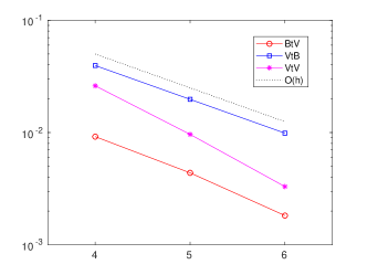
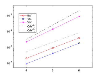
Figure 2: Errors and CPU times for the potential calculation versus the mesh refinement level.

The order of the Gauss-Legendre rule for the nearfield critically influences the cost and accuracy of the overall algorithm. In our implementation, we use a fixed quadrature order in the finest level. For the coarser level nearfield interactions of the VtV algorithm, the order is increased in each level.

As it is apparent from figure 2 the errors of all potential calculations converge at the expected $O(h)$ rate, the VtV result appears faster, probably because the multipole error in (29) gives smaller estimates for volumes. The timing of the VtB and BtV methods are in excellent agreement with the theoretical $O(h^{-2})$ estimate. The data for the VtV algorithm is somewhat higher, but considerably better than $O(h^{-3})$. A likely cause is that this algorithm evaluates nearfield interactions in coarser levels. However, in table 1 it is apparent that the number of leaves behaves pre-asymptotically in the coarser levels, and therefore the calculated number of levels are not yet sufficient exhibit the expected $O(h^{-2})$ complexity.

References

• [1] T. Askham and A.J. Cerfon. An adaptive fast multipole accelerated Poisson solver for complex geometries. J. Comput. Phys., 344:1–22, 2017.
• [2] K. E. Atkinson. The numerical evaluation of particular solutions for Poisson’s equation. IMA J. Numer. Anal., 5:319–338, 1985.
• [3] M. Bebendorf. Hierarchical Matrices: A Means to Efficiently Solve Elliptic Boundary Value Problems. Springer, 2008.
• [4] S. Börm, L. Grasedyck, and W. Hackbusch. Introduction to hierarchical matrices with applications. Engrg. Anal. Boundary Elements, pages 405 – 422, 2002.
• [5] W. Dahmen, H. Harbrecht, and R. Schneider. Adaptive methods for boundary integral equations: Complexity and convergence estimates. Math. Comp., 76(259):1243––1274, 2007.
• [6] F. Etheridge and L. Greengard. A new fast-multipole accelerated Poisson solver in two dimensions. SIAM J. Sci. Comput., 23(3):741—760, 2001.
• [7] L. Greengard and V. Rokhlin. A fast algorithm for particle simulations. J. Comput. Phys., 73:325–348, 1987.
• [8] W. Guan, Y. Jiang, and Y. Xu. Computing the newton potential in the boundary integral equation for the Dirichlet problem of the Poisson equation. J. Integral Eq. Appl, 32(3):293–324, 2021.
• [9] G. C. Hsiao and W. L. Wendland. Boundary Integral Equations, volume 168 of Applied Mathematical Sciences. Springer, 2008.
• [10] M. Ingber, A. Mammoli, and M. Brown. A comparison of domain integral evaluation techniques for boundary element method. Internat. J. Numer. Methods Engrg., 52:417–432., 2001.
• [11] J.Bey. Tetrahedral grid refinement. Computing, 55:355––378, 1995.
• [12] B.N. Khoromskij and J.M. Melenk. Boundary concentrated finite element methods. SIAM J. Numer. Anal., 41(1):1–36, 2003.
• [13] T. Koornwinder. Two-variable analogues of the classical orthogonal polynomials. In R.A. Askey, editor, Theory and Applications of Special Functions, page 435–495. Academic Press, 1975.
• [14] A. McKenny, L. Greengard, and A. Mayo. A fast Poisson solver for complex geometries. J. Comput. Phys., 118:348–355, 1995.
• [15] W. McLean. Strongly elliptic systems and boundary integral equations. Cambridge University Press, Cambridge, 2000.
• [16] S. Mohyaddin. A Fast Method For Computing Volume Potentials In The Galerkin Boundary Element Method In 3D Geometries. PhD thesis, Southern Methodist University, 2021.
• [17] K. Nabors, F.T. Korsmeyer, F.T. Leighton, and J. White. Preconditioned, adaptive, multipole-accelerated iterative methods for three-dimensional first-kind integral equations of potential theory. SIAM J. Sci. Comput., 15(3):713–735, 1994.
• [18] G. Of, O. Steinbach, and P. Urthaler. Fast evaluation of volume potentials in boundary element methods. SIAM J. Sci. Comput., 22(2):585–602, 2010.
• [19] P. W. Partridge, C. A. Brebbia, and L. C. Wrobel. The Dual Reciprocity Boundary Element Method. Computational Mechanics Publications, 1992.
• [20] S. Sauter and C. Schwab. Boundary Element Methods. Springer, 2011.
• [21] O. Steinbach and L. Tchoualag. Fast Fourier transform for efficient evaluation of Newton potential in BEM. Appl. Numer. Math., 81:1–14, 2014.
• [22] J. Tausch. The variable order fast multipole method for boundary integral equations of the second kind. Computing, 72(3):267–291, 2004.