A scattering theory of harmonic one-forms on Riemann surfaces

Abstract.

We construct a scattering theory for harmonic one-forms on Riemann surfaces, obtained from boundary value problems through systems of curves and the jump problem. We obtain an explicit expression for the scattering matrix in terms of integral operators which we call Schiffer operators, and show that the matrix is unitary. As a consequence of this scattering theory, we prove index theorems relating these conformally invariant integral operators to topological invariants. We also obtain a general association of positive polarizing Lagrangian spaces to bordered Riemann surfaces, which unifies the classical polarizations for compact surfaces of algebraic geometry with the infinite-dimensional period map of the universal Teichmüller space.

1. Introduction

1.1. Statement of results and literature

In this paper, we develop a theory of scattering of $L^{2}$ harmonic one-forms on Riemann surfaces. The scattering takes place in a network of curves which separate the Riemann surface in at least two connected components. The process is as follows. Let $\mathscr{R}$ be a compact surface divided by a complex $\Gamma$ of simple closed curves into surfaces $\Sigma_{1}$ and $\Sigma_{2}$. The number of curves is arbitrary, and we allow $\Sigma_{1}$ or $\Sigma_{2}$ to be disconnected. The reader may find it helpful to first imagine the case that $\Sigma_{1}$ and $\Sigma_{2}$ are connected and separated by $n$ closed curves. Given a harmonic function $h_{1}$ on $\Sigma_{1}$, it has boundary values on $\Gamma$, which in turn uniquely determine a harmonic function $h_{2}$ on $\Sigma_{2}$ with the same boundary values. We call $h_{2}$ the “overfare” of $h_{1}$ and write $h_{2}=\mathbf{O}_{1,2}h_{1}$.

For harmonic one-forms, there is a similar overfare procedure. Briefly, one finds an anti-derivative of a form $\alpha_{1}$ on $\Sigma_{1}$, applies the overfare $\mathbf{O}_{1,2}$ to the anti-derivative, and differentiates the result to obtain a form $\alpha_{2}$ on $\Sigma_{2}$. Of course, $\alpha_{1}$ need not be exact, and one must also specify the cohomological properties of the form $\alpha_{2}$. We deal with this by specifying a harmonic one-form $\zeta$ on $\mathscr{R}$ such that $\alpha_{1}-\zeta$ is exact on $\Sigma_{1}$, and let $\alpha_{2}$ be such that $\alpha_{2}-\zeta$ is exact on $\Sigma_{2}$. Thus the extra cohomological data required to specify the overfare of harmonic one-forms is identified with the finite-dimensional vector space of harmonic one-forms on $\mathscr{R}$. In general, the overfared harmonic one-form is not harmonic on the union.

In analogy with potential-well scattering on the real line, we can regard the aforementioned $\alpha_{2}$ as the form obtained from $\alpha_{1}$ through scattering. In this scattering process, the curves themselves play the role of the potential well. We assume only that the curves are quasicircles, which generically are non-rectifiable curves arising in Teichmüller theory. The holomorphic and anti-holomorphic parts play the role of the left- and right- moving solutions, and the asymptotic negative and positive directions are played by the two surfaces. The majority of the results of this work are directly related to the problem of developing various aspects of this scattering theory, including the unitarity of the scattering matrix.

We also apply this scattering theory to derive new results in the geometry of Riemann surfaces, for example index theorems for conformally invariant operators, and a generalization of polarizations to Riemann surfaces with boundary which incorporate boundary values.

We state our main results, emphasizing their geometric or analytic nature. Expanded statements, together with background and literature, will be given in separate sections ahead.

Geometric Results: We obtain

1. an explicit expression for the scattering matrix for harmonic one-forms in terms of the Schiffer operators, and that it is unitary;
   

2. an association of positive polarizing Lagrangian subspaces to bordered Riemann surfaces, which unifies the classical polarizations for compact surfaces with the infinite-dimensional Kirillov-Yuri’ev-Nag-Sullivan embedding of the universal Teichmüller space into a Lagrangian Grassmannian;
   

3. index theorems for conformally invariant integral operators related to the Riemann jump problem on $\mathscr{R}$ (which we call Schiffer operators), relating conformal invariants to topological invariants.
   

The results above require the following.

Analytic Results: We prove that

1. the boundary values of $L^{2}$ harmonic one-forms on a genus $g$ surface with $n$ borders, in a certain non-tangential sense, is the Sobolev $H^{-1/2}$ space;
   

2. conversely, the Dirichlet problem for one forms with $H^{-1/2}$ boundary values is well-posed, and the solutions are $L^{2}$ harmonic one-forms;
   

3. the overfare of harmonic functions is bounded in the following two cases:

   1. for quasicircles, with respect to the Dirichlet semi-norm when the originating surface is connected, and

   2. for more regular curves, with respect to a conformally invariant norm extending the Dirichlet semi-norm.
      

We prove these theorems in a very general analytic setting, which in the case at a hand, amounts to the assumption that the curve complex dividing the Riemann surface consists of a collection of quasicircles. Also, we use $L^{2}$ harmonic one-forms and Dirichlet-bounded harmonic functions throughout.

At first glance, one might think that the point of this manuscript could be made by developing the scattering theory with stronger regularity assumptions (say smooth curves and forms). However there are good reasons for the choices that have been made here in this paper. Two of these are geometric: all constructions are conformally invariant, and our analytic choices are necessary for applications to the Teichmüller theory. For example, an obvious next step is to show that the generalized period mapping yields coordinates on Teichmüller space; to do so will require both the choice of quasicircles and of $L^{2}$ harmonic one-forms. In the long run, the investigation of geometric structures on Teichmüller space (and its refinement, the Weil-Petersson class Teichmüller space) will require the theory on quasicircles. This will also be the case for the study of the symplectic actions by groups of boundary re-parametrizations. Another related motivation for considering quasicircles is a theorem of K. Vodopy’anov [Vodopyanov] and S. Nag-D. Sullivan [NS], that shows that the reparametrizations act by bounded symplectomorphisms precisely for quasisymmetric reparametrizations.

Applicability to geometry aside, the conditions are analytically natural. This can be seen even in the plane, where for example it can be shown that overfare exists and is bounded if and only if the curve is a quasicircle. See [Schippers_Staubach_Grunsky_expository] which gives a strong case for the analytic naturality of these conditions. It is remarkable that the conditions which are natural from the point of view of analysis, geometry, and algebra all coincide.

The main results are described in the sections below.

1.1.1. Overfare of harmonic functions

As described above, the process of overfare is as follows. Let $\mathscr{R}$ be a Riemann surface split into two pieces $\Sigma_{1}$ and $\Sigma_{2}$ by a Jordan curve or complex of curves. Given a harmonic function with $L^{2}$ derivatives on one of the pieces $\Sigma_{1}$ (a Dirichlet harmonic function), we find its boundary values. The “overfare” is the harmonic function on the other piece $\Sigma_{2}$ with the same boundary values as the original function. This is well-defined and bounded provided that the curves in the complex are quasicircles.

Here, there are two analytic problems to be resolved. The first is to define the boundary values in preparation for overfare, and the second is to show the existence and continuous dependence of the overfare. The first problem is in a certain sense independent of the boundary regularity, while the second problem is more delicate and sensitive to the regularity of the curve.

In defining the boundary values, the nature of the approach to the boundary can be defined either extrinsically in terms of the geometry of the ambient space containing the curve, or in terms of the intrinsic geometry of the region on which the function is defined. For example, since harmonic functions with $L^{2}$ derivatives are in the Sobolev space $H^{1}$ for a wide class of curves, one could consider the Sobolev trace to the boundary; in this case, one would need to take into account the regularity of the boundary for this to be defined. The possibility of dealing with boundaries that may not be rectifiable would add additional difficulties that brings one into the realm of geometric measure theory see [J], [JW]. Instead, our approach to boundary values proceeds intrinsically, in such a way that the boundary can be viewed as the ideal boundary of $\Sigma_{1}$, which does not depend on the geometry of the boundary in $\mathscr{R}$. For example, it can be regarded as an analytic Jordan curve in the double of $\Sigma_{1}$.

Our intrinsic approach to boundary values in some sense originates with H. Osborn [Osborn], who considered the boundary values of harmonic Dirichlet functions in planar domains $\Sigma_{1}$ along orthogonal trajectories of Green’s function of that domain. This is conformally invariant and hence intrinsic, and can be formulated in terms of the ideal boundary. We improve this “radial” approach by defining a kind of conformally non-tangential boundary value (referred to as CNT boundary values), in which non-tangential cones are defined in terms of “collar charts” taking collar neighbourhoods of the boundary to annuli. Then, a classical theorem of A. Beurling applies to show that the boundary values exist except on a Borel set of logarithmic capacity zero in the circle under the chart (we call this a null set). We show that this notion of boundary value is independent of the choice of collar chart; this is essentially because the angle of approach to the ideal boundary is a well-defined conformal invariant. Thus we show that the boundary values are defined not just along orthogonal trajectories of Green’s function but along any non-tangentially approaching curve. The independence of the boundary values on the choice of collar chart is a key tool in the application of the cutting and sewing approach to boundary value problems which we have developed in this and other papers [Schippers_Staubach_transmission], [Schippers_Staubach_Plemelj].

On the other hand, the overfare process is extrinsic, because the regularity of the boundary curve is crucial. We work with quasicircles; there are several reasons for this choice. The first is geometric: at a foundational level, Teichmüller theory of bordered surfaces involves viewing these surfaces as subsets of compact surfaces bounded by quasicircles. Classically, this is seen in the quasi-Fuschsian model of Teichmüller space [Nagbook]; for example, the universal Teichmüller space can be viewed as the set of (normalized) planar domains bounded by quasicircles. The first author’s work with D. Radnell [RadnellSchippers_monster], [RS_fiber] also shows that the Teichmüller space can be modelled as the set of surfaces capped by domains bounded by quasicircles, and that this leads to a natural fibre structure on Teichmüller space. Thus, in this work, we choose quasicircles in order to have sufficient generality in order to provide the groundwork for applying our results to Teichmüller theory.

The second reason for choosing quasicircles is analytic. The authors showed in [Schippers_Staubach_transmission_sphere] that in the Riemann sphere, the overfare exists and is bounded precisely for quasicircles. This follows from a theorem of Nag-Sullivan/Vodopy’anov that shows that quasisymmetries are precisely the bounded composition operators on the homogeneous Sobolev space $\dot{H}^{1/2}$ on the circle. As we will see ahead, this also relates to several characterizations of quasicircles in terms of the Cauchy-type and Schiffer integral operators which play the main role in this paper. A survey of such results in the Riemann sphere can be found in [Schippers_Staubach_Grunsky_expository].

It should also be noted that the Sobolev theory techniques by themselves are not sufficient in dealing with all aspects of the boundary value problems that are involved in this paper, since Sobolev spaces involve functions defined up to sets of Lebesgue measure zero. In fact, one needs to establish that boundary values exist up to a set which maps under a collar chart to a Borel set of logarithmic capacity zero in the unit circle. We call such sets null sets. By our earlier results, for quasicircles, a set which is null with respect to a collar chart on one side of the curve must be null with respect to a collar chart on the other side. This fact is central to establishing a well-defined overfare of harmonic functions. However, the claim fails if in the discussion above one replaces capacity zero with Lebesgue measure zero on the circles. Thus Sobolev theory on its own is not sufficient.

In this paper, we extend our previous overfare results to Riemann surfaces divided by many curves, rather than just a single curve. There is an obstacle to doing so. If the region $\Sigma_{2}$ is bounded by several curves, but $\Sigma_{1}$ is not connected, then the Dirichlet semi-norm is not controlled by the Dirichlet norm of the input. This is because one may add different constants to different connected components of $\Sigma_{1}$, driving up the semi-norm of the overfare, while the Dirichlet norm on the originating surface is unchanged. If the originating surface is connected, this issue does not arise, and we are able to prove boundedness of overfare with respect to the Dirichlet seminorm.

One can also obtain boundedness with respect to a genuine norm if more regularity is assumed. We introduce a conformally invariant norm: rather than adding the $L^{2}$ norm of the function as in Sobolev theory, we add an integral of the function around a boundary curve. With no connectivity assumptions, we obtain boundedness of overfare with respect to this conformally invariant norm, for curves with greater regularity. It suffices that the quasicircles are so-called Weil-Petersson quasicircles. For both of these results, in this paper we use a more flexible method of proof than in [Schippers_Staubach_transmission], and make systematic use of boundedness of the so-called bounce operator (see Definition 3.23).

1.1.2. Dirichlet boundary value problem for $L^{2}$ one-forms boundary values

A classical formulation of the Dirichlet problem on Riemannian manifolds with smooth boundary is as follows:

Let $M$ be a smooth, connected, compact, Riemannian manifold of real dimension $m$ and consider some arbitrary smooth domain $\Omega\subseteq M$ with non-empty boundary. Assume that $f\in L^{2}\left(\partial\Omega,\wedge^{k}TM\right)$, $0\leq k\leq m,$ where $L^{2}\left(\partial\Omega,\wedge^{k}TM\right)$ denotes the space of $k$-forms which are $L^{2}$ on the boundary of $\Omega$. Denoting the Hodge Laplacian by $\Delta=d\delta+\delta d$ (where $d$ is the exterior differentiation and $\delta$ its adjoint with respect to the Riemannian metric of $M$), the Dirichlet boundary value problem with boundary data $f$ is

(1.1) $$\left\{\begin{array}[]{l}u\in C\left(\Omega,\wedge^{k}TM\right)\\ \Delta u=0\text{ in }\Omega\\ \left.u\right|_{\partial\Omega}=f\text{ on }\partial\Omega\end{array}\right.$$

For $0\leq k\leq m$, this problem was studied by G. Duff and D. Spencer [DS1], [DS2], [Du3], [Sp], C. Morrey and J. Eells [ME1], [ME2], and G. Schwarz [Sch]. Through these investigations, it is known that for any $f\in L^{2}\left(\partial\Omega,\wedge^{k}TM\right)$ the Dirichlet problem has a unique solution $u\in H^{1/2}\left(\Omega,\wedge^{k}T\mathcal{M}\right)$ (Sobolev $\frac{1}{2}$-space), and moreover there exists $C>0$ independent of $f$ such that

(1.2) $$\|u\|_{H^{1/2}\left(\Omega,\wedge^{k}TM\right)}\leq C\|f\|_{L^{2}\left(\partial\Omega,\wedge^{k}TM\right)}.$$

Another well-known fact is that if $k=0$, $u\in L^{2}(\Omega)$ and $\Delta u\in L^{2}(\Omega)$ then $u|_{\partial\Omega}\in H^{-1/2}(\partial\Omega).$

In this paper we investigate the well-posedness of (1.1) when $k=1$ and $f$ in the Sobolev space of forms $H^{-1/2}\left(\partial\Sigma,\wedge^{k}T\Sigma\right)$, where $\Sigma$ is a bordered Riemann surface. This amounts to the demonstration of the fact that for an element of $f\in H^{-1/2}$ together with sufficient cohomological data, there always exists a unique $u\in L^{2}$ harmonic one-form on $\Sigma$ with boundary value $f$. We also show that $u$ depends continuously on $f$, i.e. the analogue of (1.2) is valid in this setting.

The problem for $H^{-1/2}$ boundary values is solved by reformulating the $H^{-1/2}$-space conformally invariantly, and using the theory of CNT boundary values, mentioned above. That is, we show that elements of $H^{-1/2}$ can be represented by equivalence classes of $L^{2}$ harmonic one-forms defined in collar neighbourhoods. Using the fact that $H^{-1/2}$ is the dual space to $H^{1/2}$, we will show that there is a one-to-one correspondence between elements of $H^{-1/2}$ and such equivalence classes, and this allows us to use the theory of conformally nontangential boundary values to solve the problem. It turns out that anti-derivatives of such forms have well-defined boundary values in the conformally nontangential sense, which after removing a period, can be identified with elements of $H^{1/2}$. In this context, the so-called anchor lemmas (Lemmas 3.14 and 3.15) are of fundamental importance since they imply that the limiting integral of $f\in H^{1/2}$ against any $\alpha\in\mathcal{A}(A)$ ($\mathcal{A}(A)$ is the Bergman space of holomorphic one forms on $A$, and $A$ is a collar neighbourhood of the boundary) exists and depends only on the CNT boundary values of $f$.

1.1.3. Calculus of Schiffer operators, cohomology, and index theorems

The cornerstone of this paper is the theory of certain integral operators of Schiffer. These integral operators are integral operators on holomorphic and anti-holomorphic one-forms, whose integral kernels are the two possible second derivatives of Green’s function, often called the Bergman and Schiffer kernels. These are defined as follows. Let $\mathscr{R}$ be a compact Riemann surface split into two surfaces $\Sigma_{1}$ and $\Sigma_{2}$ by a collection of Jordan curves. Let $\mathscr{G}(w;z,q)$ be Green’s function of $\mathscr{R}$ (the fundamental harmonic function with logarithmic singularities at $z$ and $q$ of opposite weight, defined up to an additive constant). We have, denoting the Bergman space of holomorphic one-forms on $\Sigma_{k}$ by $\mathcal{A}(\Sigma_{k})$ for $k=1,2$,

$$\mathbf{T}_{1,k}:\overline{\mathcal{A}(\Sigma_{1})} \rightarrow\mathcal{A}(\Sigma_{k})$$

$$\overline{\alpha} \mapsto\iint_{\Sigma_{1}}\partial_{w}\partial_{z}\mathscr{G}(w;z,q)\wedge_{w}\overline{\alpha(w)}.$$

The two choices of $k$ are obtained by restricting $z$ to $\Sigma_{k}$. If $k=1$, this has a singularity and can be treated as a Calderón-Zygmund singular integral operator. We also have the operator

$$\mathbf{S}_{1}:{\mathcal{A}(\Sigma_{1})} \rightarrow\mathcal{A}(\mathscr{R})$$

$$\overline{\alpha} \mapsto\iint_{\Sigma_{1}}\overline{\partial}_{w}\partial_{z}\mathscr{G}(w;z,q)\wedge_{w}\overline{\alpha(w)}.$$

We may of course switch the roles of $1$ and $2$ above. These were investigated extensively by M. Schiffer with various co-authors [BergmanSchiffer] [Schiffer_first], in relation to potential theory and conformal mapping, eventually culminating in a comparison theory of domains [Courant_Schiffer]. The Schiffer kernel is closely related to the so-called fundamental bidifferential and figures in geometry of function spaces on Riemann surfaces [Eynard_notes], [Schiffer_Spencer].

By a striking result of V. Napalkov and R. Yulmukhametov [Nap_Yulm], if $\mathscr{R}$ is the Riemann sphere, and $\Sigma_{1}$ and $\Sigma_{2}$ are the two complementary components of a Jordan curve $\Gamma$ on the sphere, then the Schiffer operator $\mathbf{T}_{1,2}$ is an isomorphism if and only if $\Gamma$ is a quasicircle. This is closely related to the fact that functions can be approximated in the Dirichlet semi-norm by Faber series precisely for domains bounded by quasicircles; see [Schippers_Staubach_Grunsky_expository] for an overview. The authors showed in [Schippers_Staubach_Plemelj] that, for a compact Riemann surface divided in two by a quasicircle, $\mathbf{T}_{1,2}$ is an isomorphism on the orthogonal complement of anti-holomorphic one-forms on $\mathscr{R}$. This was further generalized by M. Shirazi to the case of many curves where all but one of the components is simply connected in [Shirazi_thesis], [Schippers_Shirazi_Staubach]. The boundedness of overfare plays a central role in the formulation and proof of this fact. This extension of the isomorphism theorem was used by the authors and Shirazi to show that one-forms on a domain in a Riemann surface bounded by quasicircles can be approximated in $L^{2}$ on a larger domain [Schippers_Shirazi_Staubach]. Approximability theorems for general $k$-differentials with respect to the conformally invariant $L^{2}$ norm and less regular boundaries were obtained by N. Askaripour and T. Barron [AskBar, AskBar2] using very different methods. So far as we know, these were the first results for nested domains on Riemann surfaces in the $L^{2}$ setting.

In this paper, we characterize the kernel and image of $\mathbf{T}_{1,2}$ in the case of a Riemann surface split by a complex of quasicircles. The main tool is an extended Plemelj-Sokthoski jump formula, which is in turn based on a relation between the Schiffer operators and a generalization of the Cauchy operator originating with H. Royden [Royden] which we call the Cauchy-Royden operator. As quasicircles are not rectifiable, we are required to define the Cauchy-Royden integral using curves which approach the boundary. In the sphere with one curve, the authors showed that the resulting Plemelj-Sokhotski jump decomposition is an isomorphism if and only if the curve is a quasicircle. The analytic issues in those papers, as in this one, are resolved by the fact that the limiting integral is the same from both sides up to constants. This in turn is a consequence of the anchor lemmas and boundedness of the bounce operator. The equality of the limiting integral from both sides is also a key geometric tool; in combination with the bounded overfare it allows one to find preimages of elements of the image of $\mathbf{T}_{1,2}$.

We further use this to investigate the cohomology of the images of $\mathbf{T}_{1,1}$, $\mathbf{T}_{1,2}$ and $\mathbf{S}$. In particular we show that for any anti-holomorphic one form $\overline{\alpha}$ in $\Sigma_{1}$, $\mathbf{T}_{1,2}\overline{\alpha}$ and $\overline{\mathbf{S}}_{1}\overline{\alpha}$ are in the same cohomology class. This simple fact is surprisingly versatile. Along with the characterization of the kernels and images of $\mathbf{T}_{1,2}$ mentioned above, we also show that in the case that $\Sigma_{1}$ and $\Sigma_{2}$ are connected, the Fredholm index of $\mathbf{T}_{1,2}$ is $g_{1}-g_{2}$ where $g_{1}$ and $g_{2}$ are the genuses of $\Sigma_{1}$ and $\Sigma_{2}$. This index theorem relates a conformal invariant (the index of $\mathbf{T}_{1,2}$) to the topological invariant $g_{1}-g_{2}$.

Finally, we derive a number of new identities for Schiffer operators and their adjoints, as well as extend identities obtained earlier in [Schippers_Staubach_Plemelj] to the case of a compact surface split by a complex of curves. These identities play a central role in the scattering theory. It should be mentioned that one of these identities is a reformulation and significant generalization of an norm identity of Bergman and Schiffer for planar domains [BergmanSchiffer]. This identity can be used to derive the Grunsky inequalities (see ahead).

1.1.4. Scattering matrix and unitarity

We define a scattering process for one-forms in the following way. The overfare process defined above for functions uniquely defines the overfare of exact one-forms from connected surfaces to arbitrary ones, by

$$\mathbf{O}^{\mathrm{e}}_{\Sigma_{1},\Sigma_{2}}:\mathcal{A}^{\mathrm{e}}_{\mathrm{harm}}(\Sigma_{1}) \rightarrow\mathcal{A}^{\mathrm{e}}_{\mathrm{harm}}(\Sigma_{2})$$

$$\alpha \mapsto d\mathbf{O}_{\Sigma_{1},\Sigma_{2}}d^{-1}$$

where $\mathbf{O}_{\Sigma_{1},\Sigma_{2}}$ is overfare of harmonic functions and $\mathcal{A}_{\mathrm{harm}}(\Sigma)$ denotes $L^{2}$ harmonic one-forms on $\Sigma$. For arbitrary one-forms on a connected surface, we specify the cohomological data as follows: let $\zeta\in\mathcal{A}_{\mathrm{harm}}(\mathscr{R})$ be a one-form such that $\alpha-\zeta$ is exact on $\Sigma_{1}$. We seek a one-form with the same boundary values as $\alpha$ and in the cohomology class of $\zeta$ on $\Sigma_{2}$. This form is

$$\mathbf{O}^{\mathrm{e}}_{\Sigma_{1},\Sigma_{2}}\left(\alpha-\left.\zeta\right|_{\Sigma_{1}}\right)+\left.\zeta\right|_{\Sigma_{2}}.$$

We call $\zeta$ a “catalyzing form”, and forms which are related by overfare via $\zeta$ compatible.

From this overfare process we define a scattering operator which takes the holomorphic parts of the compatible forms, together with the anti-holomorphic part of the catalyzing forms, and produces the anti-holomorphic parts of the compatible forms and the holomorphic part of the catalyzing form. The anti-holomorphic parts can be thought of as left moving waves, while the holomorphic parts can be thought of as right moving waves.

We give an explicit form for the scattering matrix in terms of the Schiffer operators, using the identities and cohomological results of Section 4. We furthermore show that this scattering matrix is unitary, using the adjoint identities of Section 4.

These adjoint identities can be thought of as generalizations of norm inequalities relating the Schiffer operators [BergmanSchiffer], which are themselves closely related to identities relating the Faber and Grunsky operators. However neither the unitarity of the scattering process nor the adjoint identities were recognized even in the case of the plane.

1.1.5. Polarizations and Grunsky operators

For context, we sketch the well-known classical polarization for compact surfaces. Given a compact Riemann surface $\mathscr{R}$, by the Hodge decomposition theorem, every $L^{2}$ one-form has a harmonic representative. The spaces of harmonic one-forms in turn decompose into the spaces of holomorphic and anti-holomorphic one-forms. Thus the cohomology classes of a Riemann surface are represented by the direct sum of the vector spaces of holomorphic and anti-holomorphic one-forms. This decomposition depends on the complex structure.

In complex algebraic geometry, this picture is often represented in terms of the so-called period-matrix. Given a basis of the homology, divided into $a$ and $b$ curves satisfying the usual intersection conditions, one normalizes half of the periods of the holomorphic one-forms, and encoding the remaining periods in a $g\times g$ matrix where $g$ is the genus. Most often one normalizes matrix of $a$ periods to be the identity matrix; in that case, by the Riemann bilinear relations, the matrix of $b$ periods lies in the Siegel upper half-space of symmetric matrices with positive definite imaginary part. It is also possible to represent the periods with a matrix of norm less than one (that is, a matrix in the Siegel disk). It was shown by L. Ahlfors [Ahlfors] that the period matrix can be used to give coordinates on Teichmüller space; the idea of using periods as coordinates on the moduli space goes back to B. Riemann [Riemann].

An analogue of the period map exists for the case of the Teichmüller space of the disk. Nag and Sullivan [NS], following earlier work of A. Kirillov and D. Yuri’ev in the smooth case [KY2], showed that the set of quasisymmetries of the circle acts symplectically on the space of polarizations of the set of Dirichlet-bounded harmonic functions on the disk, and that the space of polarizations can be identified with an infinite-dimensional Siegel disk. They further outlined various analogies with the classical period matrix. L. Takhtajan and L-P. Teo [Takhtajan_Teo_Memoirs] showed that this “period matrix” is in fact the Grunsky matrix, and proved that the period map is a holomorphic map of the Teichmüller space of the unit disk (which is also the universal Teichmüller space). Later, with Radnell, the authors generalized this holomorphicity to genus zero surfaces with $n$ boundary curves. All of these results demonstrate the existence of a powerful analogy with the classical period matrix. Nevertheless they do not indicate the mathematical source of the analogy, nor how to unify the classical case for compact surfaces and the case of surfaces with border.

For genus zero surfaces with $n$ boundary curves, we showed with Radnell that the graph of the Grunsky matrix gives the boundary values of the set of Dirichlet-bounded harmonic functions curves [RSS_Dirichletspace], using overfare. This was extended by M. Shirazi [Shirazi_thesis, Shirazi_Grunsky] to the genus $g$ case. In this paper, we show that by treating polarizations as decompositions of boundary values of semi-exact one-forms, all the versions of the polarizations can be viewed as special cases of a single general theorem. The unifying principle is provided by boundary values of harmonic one-forms. In particular, we show that the polarizing subspace of holomorphic one-forms on a bordered surface can be viewed as the graph of an operator in an infinite Siegel disk, from which the polarizations in both the compact case and the case of genus zero surfaces with borders can be recovered. The overfare process is a crucial part of establishing this unified picture.

The bound on the polarizing operator can be viewed as a far-reaching generalization of the Grunsky inequalities. We also show how special cases of the Grunsky inequalities can be recovered from this one.

1.2. Outline of the paper

Here we give a sparing outline of the paper.

In Section 2 we gather the preliminary material about Riemann surfaces, their boundaries, and spaces of harmonic and holomorphic functions and forms. Section 3 defines the conformally non-tangential boundary values of Dirichlet bounded harmonic functions, and proves the existence and boundedness of the overfare map. Section 4 we define and prove the basic properties of the Schiffer and Cauchy-Royden operators. Furthermore we gather a collection of identities which form the computational backbone of the paper.

Section 5 contains a full treatment of the Dirichlet problem for $L^{2}$ harmonic one-forms with $H^{-1/2}$ boundary values. This is followed by the definition and properties of the overfare process for forms in Section 6.

In Section LABEL:se:index_cohomology we derive the cohomological results about the Schiffer operator, including characterizations of the kernel and image, the generalized jump theorem, and index theorems. Section LABEL:se:scattering derives the form of the scattering matrix for harmonic one-forms and proves that it is unitary. Finally, in Section LABEL:se:period_mapping we give the generalized polarizations, and apply it to solve the boundary value problem for semi-exact $L^{2}$ harmonic one-forms on bordered surfaces. We also explain its relation to the classical Grunsky inequalities and their generalizations.

2. Preliminaries

2.1. About this section

This section gathers the definitions and basic results used throughout the paper. This includes Dirichlet spaces of functions and Bergman spaces of forms; Riemann surfaces, their boundaries and specialized charts called collar charts; sewing; Green’s functions on compact surfaces and surfaces with boundary; Sobolev spaces; and harmonic measures and boundary period matrices.

2.2. Bordered surfaces

We briefly recall the definition of a bordered surface in order to remove any ambiguity. See for example [Ahlfors_Sario] for a complete treatment.

In what follows we denote by Aa,b the annulus $\{z;\,a<|z|<b\}$.

Definition 2.1.

Let $\mathbb{C}$ denote the complex plane, let $\mathbb{H}=\{z\in\mathbb{C}:\text{Im}z>0\}$ denote the upper half plane, and let $\lx@glossaries@gls@link{main}{cl}{\leavevmode\text{cl}}\,(\mathbb{H})$ denote its closure (we will let cl denote closure throughout). We say that a connected Hausdorff topological space $\hat{\Sigma}$ is a bordered Riemann surface if there is an atlas of charts $\phi:U\rightarrow\text{cl}\,(\mathbb{H})$ with the following properties.

1. Each chart is a local homeomorphism with respect to the relative topology;

2. Every point in $\hat{\Sigma}$ is contained in the domain of some chart;

3. Given any pair of charts $\phi_{k}:U_{k}\rightarrow\text{cl}\,(\mathbb{H})$, $k=1,2$, if $U_{1}\cap U_{2}$ is non-empty, then $\phi_{1}\circ\phi_{2}^{-1}$ is a biholomorphism on $U_{1}\cap U_{2}\cap\mathbb{H}$.

This defines a distinction between interior and border points (see e.g. [Ahlfors_Sario, p23-24]). That is, we say $p$ is on the border if there is a chart in the atlas such that $\phi(p)$ is on the real axis, and $p$ is in the interior if there a chart mapping $p$ to a point in $\mathbb{H}$. In either case, if the claim holds for one chart, it holds for all of them. We will denote the set of interior points by $\Sigma$ and the set of border points by $\partial\Sigma$. We call $\partial\Sigma$ the border, and note that the border is also the topological boundary of $\Sigma$ in $\hat{\Sigma}$. Observe that $\Sigma$ is a Riemann surface in the standard sense.

We will call a chart $\phi$ which contains a boundary point in its domain a “boundary chart” or “border chart”. Now regarding the notion of the double of a bordered Riemann surface, assume that $\phi_{k}:U_{k}\rightarrow\text{cl}\,(\mathbb{H})$, $k=1,2$, are charts such that $U_{1}\cap U_{2}\cap\partial\Sigma$ is non-empty. Then by the Schwarz reflection principle, $\phi_{1}\circ\phi_{2}^{-1}$ extends to a biholomorphism of an open set containing $\phi_{2}(U_{1}\cap U_{2})$. This open set can be taken to be the union of $\phi_{2}(U_{1}\cap U_{2})$ with its reflection in the real axis. In the usual construction of the double, any chart $\phi$ which contains border points can be extended to a chart in the double by reflection. By the above argument, the overlap map $\phi_{1}\circ\phi_{2}^{-1}$ for any pair $\phi_{1},\phi_{2}$ of such extensions is a biholomorphism. This defines the atlas on the double of $\Sigma$ which is denoted here by $\Sigma^{d}$.

Remark 2.2.

Once the border structure is established as above, for convenience we will allow interior charts to have image in $\mathbb{C}$ and not necessarily in $\mathbb{H}$. Moreover, we will also consider border charts which map into the closure of the disk $\mathbb{D}^{+}=\{z\in\bar{\mathbb{C}}:|z|<1\}$, with border points mapping to $|z|=1$. Every such chart is a border chart in the original sense after composition by a Möbius transformation.

One of our main objects of study is a particular type of bordered Riemann surface which is defined as follows:

Definition 2.3.

We say that $\Sigma$ is a bordered Riemann surface of type $(g,n),$ if it is bordered (in the sense Definition 2.1), the border has $n$ connected components, each of which is homeomorphic to $\mathbb{S}^{1}$, and its double $\Sigma^{d}$ is a compact surface of genus $2g+n-1$.

Visually, a bordered surface of type $(g,n)$ is a $g$-handled surface bounded by $n$ simple closed curves. We order the borders and label them accordingly, so that $\partial\Sigma=\partial_{1}\Sigma\cup\cdots\cup\partial_{n}\Sigma$. The borders can be identified with analytic curves in the double $\Sigma^{d}$, and we denote the union $\Sigma\cup\partial\Sigma$ by $\text{cl}(\Sigma)$.

Finally, we observe that borders are conformally invariant. That is, if $\Sigma_{1}$ and $\Sigma_{2}$ are bordered surfaces, then any biholomorphism $f:\Sigma_{1}\rightarrow\Sigma_{2}$ extends to a homeomorphism of the borders. In fact, $f$ extends to a biholomorphism between the doubles $\Sigma_{1}^{d}$ and $\Sigma_{2}^{d}$ which takes $\partial\Sigma_{1}$ to $\partial\Sigma_{2}$. Finally, if only one of the two surfaces has a border, say $\Sigma_{1}$, then one can endow $\Sigma_{2}$ with a border using $f$. In particular, there is a unique maximal border structure.

Remark 2.4.

Note that if $\Sigma$ has type $(g,n)$, the border structure is maximal, since $\Sigma^{d}$ is a compact surface.

Definition 2.5.

We say that a homeomorphic image $\Gamma$ of $\mathbb{S}^{1}$ is a strip-cutting Jordan curve if it is contained in an open set $U$ and there is a biholomorphism $\phi:U\rightarrow\mathbb{A}_{r,R}$ for some annulus

$$\mathbb{A}_{r,R}\subset\mathbb{C},\ \ \ r<1<R,$$

in such a way that $\phi(\Gamma)$ is isotopic to the circle $|z|=1.$ We call $U$ a doubly-connected neighbouhood of $\Gamma$ and $\phi$ a doubly-connected chart.

Remark 2.6.

If $\Gamma$ is a strip-cutting curve, by shrinking $\mathbb{A}_{r,R}$, we can assume that (1) $\phi$ extends biholomorphically to an open neighourhood of $\text{cl}\,(U)$, (2), that the boundary curves of $U$ are themselves strip cutting (in fact analytic), and (3) that $\Gamma$ is isotopic to each of the boundary curves (using $\phi^{-1}$ to provide the isotopy).

Remark 2.7.

An analytic Jordan curve is by definition strip-cutting.

Throughout the paper we consider nested Riemann surfaces. That is, we are given a type $(g,n)$ bordered surface $\Sigma$, another Riemann surface $\mathscr{R}$ which is compact, and a holomorphic inclusion map $\iota(\Sigma)\subset\mathscr{R}$. Assume that the closure of $\Sigma$ is compact in $R$, and furthermore the boundary consists of $n$ closed strip-cutting Jordan curves, which do not intersect. In that case, the inclusion map $\iota$ extends homeomorphically to a map from the border to the strip-cutting Jordan curves. Thus $\partial\Sigma$ is in one-to-one correspondence with its image under the homeomorphic extension of $\iota$, and in fact the image is the boundary of $\iota(\Sigma)$ in the ordinary topological sense. For this reason, we will not notationally distinguish $\Sigma$ from $\iota(\Sigma)$. We will also use the notation $\partial\Sigma$ for both the boundary of $\iota(\Sigma)$ in $\mathscr{R}$ and the abstract border of $\Sigma$, and denote both closures by $\text{cl}\,(\Sigma)$.

In fact, the assumption that the surface $\Sigma$ is bordered can be removed in the following way.

Theorem 2.8.

Let $\Sigma$ be an open connected subset of a Riemann surface $\mathscr{R}$. Assume that the topological boundary of $\Sigma$ in $\mathscr{R}$ is a finite collection $\Gamma=\Gamma_{1}\cup\cdots\cup\Gamma_{n}$ of strip-cutting Jordan curves. Furthermore suppose that there are doubly-connected charts $\phi_{k}:U_{k}\rightarrow\mathbb{A}_{k}$ of $\Gamma_{k}$ for $k=1,\ldots,n$ $($where $\mathbb{A}_{k}$’s are annuli$)$ such that the closures of $U_{k}$ are mutually disjoint, and $U_{k}\backslash\Gamma$ consists of two connected components, one of which is entirely contained in $\Sigma$ and one which is in $\mathscr{R}\backslash\Sigma$. Then $\Sigma$ is a bordered surface and the inclusion map is a homeomorphism.

Proof.

First, observe that $\Sigma$ has a unique complex structure compatible with $\mathscr{R}$, so we let $\mathscr{A}$ be an atlas compatible with this structure.

Let $U_{k}^{+}$ denote the component of $U_{k}\backslash\Gamma$ in $\Sigma$. Then $\phi_{k}(U_{k}^{+})$ is an open subset of $\mathbb{C}$ bounded by two Jordan curves, one of which is a boundary $\gamma$ of $\mathbb{A}_{k}$ and one of which is the Jordan curve $\phi_{k}(\Gamma)$. By [ConwayII, Theorems 3.3, 3.4 Sect 15.3], there is a biholomorphism $\psi_{k}:\phi_{k}(U_{k}^{+})\rightarrow\mathbb{A}_{r,1}$ which extends to a homeomorphism of the boundaries, taking $\gamma$ to $|z|=r$ and $\phi_{k}(\Gamma)$ to $\mathbb{S}^{1}$. Adjoining the points in $\Gamma_{k}$ to $\Sigma$, Then

$$\mathscr{A}\cup\left\{\left.\psi_{1}\circ\phi_{1}\right|_{U_{1}^{+}},\ldots,\left.\psi_{n}\circ\phi_{n}\right|_{U_{n}^{+}}\right\}$$

is an atlas making $\Sigma\cup\partial\Sigma$ into a bordered surface. ∎

Remark 2.9.

The embedding of the border $\partial\Sigma$ in $\mathscr{R}$ need not be regular. That is, the inclusion map does not extend to a smooth or analytic map from $\partial\Sigma$ onto its image under inclusion $\iota$, unless the image consists of smooth or analytic curves.

By another application of [ConwayII, Theorems 3.3, 3.4 Sect 15.3], it is easily shown that if $\Sigma_{1}\subset\mathscr{R}_{1}$ and $\Sigma_{2}\subset\mathscr{R}_{2}$ satisfy the conditions above, and $f:\Sigma_{1}\rightarrow\Sigma_{2}$ is a biholomorphism, then $f$ extends continuously to a map taking each Jordan curve in $\partial\Sigma_{1}$ homeomorphically to one of the Jordan curves of $\partial\Sigma_{2}$.

It is helpful to have the following distinction in mind throughout the paper: certain statements are “intrinsic” while others are “extrinsic”. Intrinsic statements about a Riemann surface $\Sigma$ are those which depend only on the surface itself and are unchanged under a biholomorphism. For example, the border is intrinsic, and the harmonic function which is one on $\partial_{k}\Sigma$ and $0$ on other curves is intrinsic. Extrinsic statements about a Riemann surfaces $\Sigma$ nested in another surface $\mathscr{R}$, are those which make reference to $\mathscr{R}$. For example, “strip-cutting” is an extrinsic property, as is the regularity of $\iota(\partial\Sigma)$. An example of an extrinsic object is the restriction of Green’s function of $\mathscr{R}$ to $\Sigma$ (see the next subsection for the definition of Green’s functions).

When dealing with intrinsically phrased boundary value problems, regularity of the boundary is not an issue, since we can treat the boundary as a border and thus we have its analytic structure at our disposal. Examples of this are the Dirichlet problem (as we phrase it) in Section 5 and CNT boundary values of $L^{2}$ harmonic forms on $\Sigma$ in Section 3.2. On the other hand, when dealing with extrinsically phrased boundary value problems, regularity of the boundary is a major concern. Overfare/Transmission phenomena in Section 3.5, in which the boundary values of a harmonic function on $\Sigma$ become data for the Dirichlet problem on $\mathscr{R}\backslash\Sigma$, are of this nature, as are the Schiffer operators and results regarding them in Section 4 and onward.

2.3. Collar charts

We also define a kind of chart on bordered surfaces near the boundary, which we call a collar chart.

Definition 2.10.

Let $\Sigma$ be a bordered Riemann surface of type $(g,n)$. A biholomorphism $\phi:U\rightarrow\mathbb{A}_{r,1}$ is called a collar chart of $\partial_{k}\Sigma$ (for some fixed $k$) if $U$ is an open set in $\Sigma$ bounded by two Jordan curves $\partial\Sigma$ and $\Gamma$, such that $\Gamma$ is isotopic to $\partial_{k}\Sigma$ within the closure of $U$, and such that $\phi$ extends continuously to the closure. A domain $U$ is a collar neighbourhood of $\partial_{k}\Sigma$ if it is the domain of some collar chart.

Proposition 2.11.

Let $\Sigma$ be a type $(g,n)$ surface. Then every boundary curve $\partial_{k}\Sigma$ has a collar chart.

Proof.

Let $\Sigma^{d}$ be the double of $\Sigma$, so that each boundary $\partial_{k}\Sigma$ is an analytic Jordan curve and hence strip-cutting. Let $U_{k}$, $U_{k}^{+}$, $\phi_{k}$ and $\psi_{k}$ be as in the proof of Theorem 2.8. Then $\left.\psi_{k}\circ\phi_{k}\right|_{U_{k}^{+}}$ is a collar chart. ∎

Furthermore, we have the following consequence of Carathéodory’s theorem.

Theorem 2.12.

Let $\Sigma$ be a bordered surface and $\Gamma$ be a component of the border which is homeomorphic to $\mathbb{S}^{1}$. If $\phi:U\rightarrow\mathbb{A}$ is a collar chart, then $\phi$ extends continuously to $\partial_{k}\Sigma$. The extension is a homeomorphism of $\partial_{k}\Sigma$ onto $\mathbb{S}^{1}$.

Proof.

$\Gamma$ is an analytic Jordan curve in the double, and hence strip-cutting. Let $\psi:V\rightarrow\mathbb{A}$ be a doubly-connected chart for $\Gamma$. By shrinking $V$ we may assume that the boundaries of $\psi(V)$ are Jordan curves. Then $\psi\circ\phi^{-1}$ maps $\mathbb{A}$ onto a doubly-connected region bounded by Jordan curves, so the claim follows from [ConwayII, Theorems 3.4 Sect 15.3]. ∎

To keep the notation simple, we will also denote the continuous extension by $\phi$.

Remark 2.13 (Isotopy and extension).

By shrinking $r$, for any collar chart $\phi:U\rightarrow\mathbb{A}_{1,r}$ we can always assume that the inner boundaries are analytic curves and $\phi$ has an analytic extensions to these curves. Furthermore, $H(t,\theta)=\phi^{-1}(e^{t}e^{i\theta})$ defines an isotopy between the level curve $|\phi|=r$ and $\partial_{k}\Sigma$, running through the level curves of $|\phi|$.

In fact the homeomorphic extension is analytic on the border. This can be phrased in various ways, one of which is as follows. Treat $\Sigma$ as a subset of its double $\Sigma^{d}$ with involution $\tilde{(\cdot)}$. For a collar neighbourhood $U$ of $\partial_{k}\Sigma$, let $U^{d}=U\cup\tilde{U}\cup\partial_{k}\Sigma$. We then have

Proposition 2.14.

Let $\phi:U\rightarrow\mathbb{A}_{r,1}$ be a collar chart. Let $U^{d}=U\cup\tilde{U}\cup\partial_{k}\Sigma$ be the double of $U$. If $\Sigma$ is included in its double $\Sigma^{d}$, then $\phi$ extends to a doubly-connected chart $\phi^{d}$ of $\partial_{k}\Sigma$ mapping $U^{d}$ onto the annulus $\mathbb{A}_{r,1/r}$ satisfying $\phi^{d}(\tilde{z})=1/\overline{\phi^{d}(z)}$.

Remark 2.15.

In particular, the border charts give a well-defined meaning to continuous, $C^{k}$, analytic functions, vector fields, one-forms and so forth, on $\partial_{k}\Sigma$ for $k=1,\ldots,n$. For example, a one-form $\alpha$ on $\partial_{k}\Sigma$ is continuous, $C^{k}$, or analytic if its expression in a boundary chart $\psi:U\rightarrow\mathbb{H}$ near $p$ is $h(x)\,dx$ where $h$ is continuous, $C^{k}$ or analytic respectively, and this holds for all $p\in\partial_{k}\Sigma$. If the property holds for any collection of boundary charts covering $\partial_{k}\Sigma$ then it holds for all boundary charts. Thus, it is enough that the property in question holds for one collar chart; that is, $\alpha$ is continuous, $C^{k}$, or analytic if and only if in the local coordinates defined using $\left.\phi\right|_{\partial_{k}\Sigma}$ for a collar chart $\phi$, $\alpha$ is given by $h(e^{i\theta})\,d\theta$ where $h$ is respectively continuous, $C^{k}$ or analytic on $\mathbb{S}^{1}$.

Finally, we have the following useful fact.

Proposition 2.16.

Let $\Sigma$ be a Riemann surface with border $\Gamma$ homeomorphic to $\mathbb{S}^{1}$, and let $U$ and $V$ be collar neighbourhoods of a boundary curve $\partial_{k}\Sigma$. There is a collar chart $\phi:W\rightarrow\mathbb{A}_{r,1}$ such that $W\subseteq U\cap V$. Moreover $r$ can be chosen so that the inner boundary of $W$ is contained in $U\cap V$.

Proof.

By Remark 2.13 we can choose collar neighbourhoods $U^{\prime}$ and $V^{\prime}$ whose inner boundaries are analytic curves $\gamma_{1}$ and $\gamma_{2}$ contained in $U$ and $V$, with corresponding collar charts $\psi_{U^{\prime}}$ and $\psi_{V^{\prime}}$ extending analytically to $\gamma_{1}$ and $\gamma_{2}$. By composing with $\psi_{U^{\prime}}$, we can assume that $\Gamma=\mathbb{S}^{1}$, $\psi_{U^{\prime}}(z)=z$, $U^{\prime}=\mathbb{A}_{r,1}$ for some $r$, and $\gamma_{1}=\{z:|z|=r\}$.

Now let $M$ be the maximum value of $|\psi_{V^{\prime}}(z)|$ on $\gamma_{2}$, which exists because $\gamma_{2}$ is compact. In that case $\text{cl}\,(\mathbb{A}_{{s},1})\subseteq V^{\prime}\cap U^{\prime}$ for $s=(1+M)/2$. We may now choose $W=\mathbb{A}_{{s},1}$ and $\phi(z)=z$ to prove the claim. ∎

Proposition 2.17.

Let $\Gamma$ be a strip-cutting Jordan curve in $\mathscr{R}$, and let $\phi:U\rightarrow\mathbb{A}_{r,R}$ be a doubly-connected chart. There are canonical collar charts $\psi_{k}:U_{k}\rightarrow\mathbb{A}$ with $U_{k}\subseteq U\cap\Sigma_{k}$ for $k=1,2$. $U_{k}$ may be chosen so that their inner boundaries are analytic curves contained in $U$.

Proof.

Applying the proof of Theorem 2.8 to each side of $\Gamma$ we obtain the desired $\psi_{k}$. ∎

2.4. Function spaces and holomorphic and harmonic forms

In this paper, we will denote positive constants in the inequalities by $C$ whose value is not crucial to the problem at hand. The value of $C$ may differ from line to line, but in each instance could be estimated if necessary. Moreover, when the values of constants in our estimates are of no significance for our main purpose, then we use the notation $a\lesssim b$ as a shorthand for $a\leq Cb$. If $a\lesssim b$ and $b\lesssim a$ then we write $a\approx b.$

On any Riemann surface, define the dual of the almost complex structure, $\ast$ in local coordinates $z=x+iy$, by

$$\ast(a\,dx+b\,dy)=a\,dy-b\,dx.$$

This is independent of the choice of coordinates. It can also be computed in coordinates that for any complex function $h$

(2.1) $$2\partial_{z}h=dh+i\ast dh.$$

Definition 2.18.

We say a complex-valued function $f$ on an open set $U$ is harmonic if it is $C^{2}$ on $U$ and $d\ast df=0$. We say that a complex one-form $\alpha$ is harmonic if it is $C^{1}$ and satisfies both $d\alpha=0$ and $d\ast\alpha=0$.

Equivalently, harmonic one-forms are those which can be expressed locally as $df$ for some harmonic function $f$. Harmonic one-forms and functions must of course be $C^{\infty}$.

Denote complex conjugation of functions and forms with a bar, e.g. $\overline{\alpha}$. A holomorphic one-form is one which can be written in coordinates as $h(z)\,dz$ for a holomorphic function $h$, while an anti-holomorphic one-form is one which can be locally written $\overline{h(z)}\,d\bar{z}$ for a holomorphic function $h$.

Denote by $L^{2}(U)$ the set of one-forms $\omega$ on an open set $U$ which satisfy

$$\iint_{U}\omega\wedge\ast\overline{\omega}<\infty$$

(observe that the integrand is positive at every point, as can be seen by writing the expression in local coordinates). This is a Hilbert space with respect to the inner product

(2.2) $$(\omega_{1},\omega_{2})=\iint_{U}\omega_{1}\wedge\ast\overline{\omega_{2}}.$$

Definition 2.19.

The Bergman space of holomorphic one forms is

(2.3) $$\lx@glossaries@gls@link{main}{bergman}{\leavevmode\mathcal{A}}(U)=\{\alpha\in L^{2}(U)\,:\,\alpha\ \text{holomorphic}\}.$$

The anti-holomorphic Bergman space is denoted $\overline{\mathcal{A}(U)}$. We will also denote

(2.4) $$\lx@glossaries@gls@link{main}{Aharm}{\leavevmode\mathcal{A}_{\mathrm{harm}}}(U)=\{\alpha\in L^{2}(U)\,:\,\alpha\ \text{harmonic}\}.$$

Observe that $\mathcal{A}(U)$ and $\overline{\mathcal{A}(U)}$ are orthogonal with respect to the inner product (2.2). In fact we have the direct sum decomposition

(2.5) $$\mathcal{A}_{\mathrm{harm}}(U)=\mathcal{A}(U)\oplus\overline{\mathcal{A}(U)}.$$

If we restrict the inner product to $\alpha,\beta\in\mathcal{A}(U)$ then since $\ast\overline{\beta}=i\overline{\beta}$, we have

$$(\alpha,\beta)=i\iint_{U}\alpha\wedge\overline{\beta}.$$

Denote the projections induced by this decomposition by

$$\mathbf{P}_{U}:\mathcal{A}_{\mathrm{harm}}(U) \rightarrow\mathcal{A}(U)$$

(2.6) $$\overline{\mathbf{P}}_{U}:\mathcal{A}_{\mathrm{harm}}(U) \rightarrow\overline{\mathcal{A}(U)}.$$

Let $f:U\rightarrow V$ be a biholomorphism. We denote the pull-back of $\alpha\in\mathcal{A}_{\mathrm{harm}}(V)$ under $f$ by $f^{*}\alpha.$ Explicitly, if $\alpha$ is given in local coordinates $w$ by $a(w)\,dw+\overline{b(w)}\,d\bar{w}$ and $w=f(z),$ then the pull-back is given by

$$f^{*}\left(a(w)\,dw+\overline{b(w)}\,d\bar{w}\right)=a(f(z))f^{\prime}(z)\,dz+\overline{b(f(z))}\overline{f^{\prime}(z)}\,d\bar{z}.$$

The Bergman spaces are all conformally invariant, in the sense that if $f:U\rightarrow V$ is a biholomorphism, then $f^{*}\mathcal{A}(V)=\mathcal{A}(U)$ and this preserves the inner product. Similar statements hold for the anti-holomorphic and harmonic spaces.

Definition 2.20.

We define the space $\lx@glossaries@gls@link{main}{exactA}{\leavevmode\mathcal{A}^{\mathrm{e}}}_{\mathrm{harm}}(U)$ as the subspace of exact elements of $\mathcal{A}_{\mathrm{harm}}(U)$, and similarly for $\mathcal{A}^{\mathrm{e}}(\Sigma)$ and $\overline{\mathcal{A}^{\mathrm{e}}(\Sigma)}$.

The following spaces also play significant roles in this paper.

Definition 2.21.

The Dirichlet spaces of functions are defined by

$$\lx@glossaries@gls@link{main}{Dharm}{\leavevmode\mathcal{D}_{\mathrm{harm}}}(U) =\{f:U\rightarrow\mathbb{C},f\in C^{2}(U),\,:\,df\in L^{2}(U)\,\,\,\mathrm{and}\,\,\,d\ast df=0\},$$

$$\lx@glossaries@gls@link{main}{D}{\leavevmode\mathcal{D}}(U) =\{f:U\rightarrow\mathbb{C}\,:\,df\in\mathcal{A}(U)\},\ \text{and}$$

$$\overline{\mathcal{D}(U)} =\{f:U\rightarrow\mathbb{C}\,:\,df\in\overline{\mathcal{A}(U)}\}.$$

We can define a degenerate inner product on $\mathcal{D}_{\mathrm{harm}}(U)$ by

$$(f,g)_{\mathcal{D}_{\mathrm{harm}}(U)}=(df,dg)_{\mathcal{A}_{\mathrm{harm}}(U)},$$

where the right hand side is the inner product (2.2) restricted to elements of $\mathcal{A}_{\mathrm{harm}}(U)$. The inner product can be used to define a seminorm on $\mathcal{D}_{\mathrm{harm}}(U)$, by letting

$$\|f\|^{2}_{\mathcal{D}_{\mathrm{harm}}(U)}:=(df,df)_{\mathcal{A}_{\mathrm{harm}}(U)}.$$

We note that if one defines the Wirtinger operators via their local coordinate expressions

$$\partial f=\frac{\partial f}{\partial z}\,dz,\ \ \ \overline{\partial}f=\frac{\partial f}{\partial\bar{z}}\,d\bar{z},$$

then the aforementioned inner product can be written as

(2.7) $$(f,g)_{\mathcal{D}_{\mathrm{harm}}(U)}=i\iint_{U}\left[\partial f\wedge\overline{\partial g}-\overline{\partial}f\wedge\partial\overline{g}\right].$$

Although this implies that $\mathcal{D}(U)$ and $\overline{\mathcal{D}(U)}$ are orthogonal, there is no direct sum decomposition into $\mathcal{D}(U)$ and $\overline{\mathcal{D}(U)}$. This is because in general there exist exact harmonic one-forms whose holomorphic and anti-holomorphic parts are not exact.

Observe that the Dirichlet spaces are conformally invariant in the same sense as the Bergman spaces. That is, if $f:U\rightarrow V$ is a biholomorphism then

$$\lx@glossaries@gls@link{main}{cf}{\leavevmode\mathbf{C}_{f}}h=h\circ f$$

satisfies

$$\mathbf{C}_{f}:\mathcal{D}(V)\rightarrow\mathcal{D}(U)$$

and this is a semi-norm preserving bijection. If $f(p)=q$ then $\mathbf{C}_{f}$ is an isometry from $\mathcal{D}(V)_{q}$ to $\mathcal{D}(U)_{p}$. Similar statements hold for the anti-holomorphic and harmonic spaces.

We also note that if $h\in\mathcal{D}(U)$ and $\tilde{h}(z)=h\circ\phi^{-1}(z)$ is the expression for $h$ in local coordinates $z=\phi(w)$ in an open set $\phi(U)\subseteq\mathbb{C}$, then we have the local expression

$$(h,h)_{\mathcal{D}(U)}=\iint_{\phi(U)}|\tilde{h}^{\prime}(z)|^{2}dA_{z}$$

where $dA$ denotes Lebesgue measure in the plane. Similar expressions hold for the other Dirichlet spaces.

Next we gather some results from the theory of Sobolev spaces which we shall use in this paper.

Definition 2.22.

For $s\in\mathbb{R}$, one defines the Sobolev space $\lx@glossaries@gls@link{main}{sobolev}{\leavevmode H^{s}}(\mathbb{R}^{n}),$ which consists of tempered distributions $u$ such that

$$\|u\|^{2}_{H^{s}(\mathbb{R}^{n})}:=\|(1-\Delta)^{s/2}u\|^{2}_{L^{2}(\mathbb{R}^{n})}=\int_{\mathbb{R}^{n}}(1+|\xi|^{2})^{s}|\widehat{u}(\xi)|^{2}\,d\xi<\infty,$$

where $\widehat{u}(\xi)$ is the Fourier transform of $u$ defined by $\widehat{u}(\xi)=\int_{\mathbb{R}^{n}}u(x)\,e^{-ix\cdot\xi}\,dx$ and

$$(1-\Delta)^{s/2}u(x)=\frac{1}{(2\pi)^{n}}\int_{\mathbb{R}^{n}}(1+|\xi|^{2})^{s/2}\,\widehat{u}(\xi)\,e^{ix\cdot\xi}\,d\xi.$$

The homogeneous Sobolev space $\lx@glossaries@gls@link{main}{homsobolev}{\leavevmode\dot{H}^{s}}(\mathbb{R}^{n}),$ is the space of tempered distributions such that $\int_{\mathbb{R}^{n}}|\xi|^{2s}\,|\widehat{u}(\xi)|^{2}\,d\xi<\infty.$

The scales of Sobolev spaces that are of particular interest for us are $s=1,\pm\frac{1}{2}$ (defined on various manifolds). For instance $H^{1}(\mathbb{R}^{n})$ consists of the space of tempered distributions $u$ for which

(2.8) $$\begin{split}\|u\|_{H^{1}(\mathbb{R}^{n})}:=\left(\int_{\mathbb{R}^{n}}|\nabla u(x)|^{2}\,dx+\int_{\mathbb{R}^{n}}|u|^{2}dx\right)^{\frac{1}{2}}\\ =:\left(\|u\|^{2}_{\dot{H}^{1}(\mathbb{R}^{n})}+\|u\|^{2}_{L^{2}(\mathbb{R}^{n})}\right)^{\frac{1}{2}}<\infty,\end{split}$$

and $H^{1/2}(\mathbb{R}^{n})$ consists of the space of tempered distributions $u$ for which

(2.9) $$\begin{split}\|u\|_{H^{1/2}(\mathbb{R}^{n})}:=\left(\int_{\mathbb{R}^{n}}\int_{\mathbb{R}^{n}}\frac{|u(x)-u(y)|^{2}}{|x-y|^{n+1}}dxdy+\int_{\mathbb{R}^{n}}|u|^{2}dx\right)^{\frac{1}{2}}\\ =:\left(\|u\|^{2}_{\dot{H}^{1/2}(\mathbb{R}^{n})}+\|u\|^{2}_{L^{2}(\mathbb{R}^{n})}\right)^{\frac{1}{2}}<\infty.\end{split}$$

The Sobolev space $H^{s}(\mathbb{S}^{1}),$ $s\geq 0,$ will also play an important role in our investigations, whose definition we also recall. Given $f\in L^{2}(\mathbb{S}^{1})$ one defines the Fourier coefficients and the Fourier series associated to $f$ by

(2.10) $$\hat{f}(n)=\frac{1}{2\pi}\int_{0}^{2\pi}f(t)e^{-in\theta}\,d\theta,\,\,\,f=\sum_{n=-\infty}^{\infty}\hat{f}(n)e^{in\theta},\quad$$

where the convergence of the series is both in the $L^{2}$-norm and also pointwise almost everywhere. The Sobolev space $H^{s}(\mathbb{S}^{1})$ is defined by

(2.11) $$H^{s}(\mathbb{S}^{1})=\left\{\varphi\in L^{2}(\mathbb{S}^{1}):\sum_{n=-\infty}^{\infty}\left(1+|n|^{2}\right)^{s}|\hat{f}(n)|^{2}<\infty\right\}.$$

Like all other $L^{2}$-based Sobolev spaces, $H^{s}(\mathbb{S}^{1})$ is a Hilbert space and given $f,\,g\in H^{s}(\mathbb{S}^{1})$ their scalar product is given by

(2.12) $$\langle f,g\rangle_{H^{s}(\mathbb{S}^{1})}=\sum_{n=-\infty}^{\infty}\left(1+|n|^{2}\right)^{s}\hat{f}(n)\overline{\hat{g}(n)},$$

and so

(2.13) $$\|f\|_{H^{s}(\mathbb{S}^{1})}=\left(\sum_{n=-\infty}^{\infty}\left(1+|n|^{2}\right)^{s}|\hat{f}(n)|^{2}\right)^{1/2}.$$

Of particular interest in this paper, are the functions in the Sobolev space $H^{1/2}(\mathbb{S}^{1})$ for which one also has the analogue of (2.9), i.e.

(2.14) $$\|f\|_{H^{1/2}(\mathbb{S}^{1})}:=\Big{(}\int_{\mathbb{S}^{1}}\int_{\mathbb{S}^{1}}\frac{|f(z)-f(\zeta)|^{2}}{|z-\zeta|^{2}}\,|dz|\,|d\zeta|+\|f\|^{2}_{L^{2}(\mathbb{S}^{1})}\Big{)}^{1/2}.$$

As was shown by J. Douglas [Douglas], for a function $F\in\mathcal{D}_{\mathrm{harm}}(\mathbb{D})$ ($\mathbb{D}$ denotes the unit disk), then the restriction of $F$ to $\mathbb{S}^{1}$ is in $H^{1/2}(\mathbb{S}^{1})$ and if the boundary value of $F$ is denoted by $f$ then one has that

(2.15) $$\|F\|^{2}_{\mathcal{D}_{\mathrm{harm}}(\mathbb{D})}=\pi\int_{0}^{2\pi}\int_{0}^{2\pi}\frac{|{f}(z)-f(\zeta)|^{2}}{|z-\zeta|^{2}}\,|dz|\,|d\zeta|.$$

The dual of $H^{1/2}(\mathbb{S}^{1})$, identified with $H^{-1/2}(\mathbb{S}^{1})$, consists of linear functionals $L$ on $H^{1/2}(\mathbb{S}^{1})$ with the property that if $\alpha_{n}:=L(e^{in\theta})$ (this is the action of the funcional $L$ on the function $e^{in\theta}$), then

(2.16) $$\sum_{n=-\infty}^{\infty}\frac{|\alpha_{n}|^{2}}{(1+|n|^{2})^{1/2}}<\infty.$$

Moreover one has

(2.17) $$\|L\|_{H^{-1/2}(\mathbb{S}^{1})}=\sup_{\|g\|_{H^{1/2}(\mathbb{S}^{1})}=1}|\sum_{n=-\infty}^{\infty}\alpha(n)\overline{\hat{g}(n)}|.$$

We shall also recall the following useful embedding result, whose proof can be found in [Triebel].

Theorem 2.23.

Let $1\leq p<\infty$ and $s\geq 0$ with $s+\frac{1}{p}\geq\frac{1}{2}$ then one has the continuous inclusion $($embedding$)$

(2.18) $$H^{s}(\mathbb{S}^{1})\subset L^{p}(\mathbb{S}^{1}).$$

Now regarding Sobolev spaces on manifolds, we first recall the definition of Sobolev $H^{s}(M)$, $s\in\mathbb{R}$ for compact manifolds $M$, see e.g. [Booss].

Definition 2.24.

Let $M$ be an $n-$dimensional smooth compact manifold without boundary, with the smooth atlas $(\phi_{j},U_{j})$ and the corresponding smooth partition of unity $\psi_{j}$ with $\psi_{j}\geq 0$, $\mathrm{supp}\,\psi_{j}\subset U_{j}$ and $\sum_{j}\psi_{j}=1$. Given $s\geq 0,$ the Sobolev spaces $H^{s}(M)$ are the space of complex-valued $L^{2}$ functions on $M$ for which

(2.19) $$\|f\|_{H^{s}(M)}:=\sum_{j}\|(\psi_{j}f)\circ\phi^{-1}_{j}\|_{H^{s}(\mathbb{R}^{n})}<\infty.$$

The homogeneous Sobolev space $\dot{H}^{s}(M)$ is defined using (2.19) by substituting $H^{s}(\mathbb{R}^{n})$ with $\dot{H}^{s}(\mathbb{R}^{n})$.

It is also well-known that different choices of the atlas and its corresponding partition of unity, produces norms that are equivalent with (2.19).

Next let $X$ be a smooth compact $n$-dimensional manifold with smooth boundary $\mathrm{bd}(X)$ and fix a Riemannian structure on $X$. Use the Riemannian structure to construct a collar neighbourhood $N=\mathrm{bd}(X)\times I$ of the boundary $\mathrm{bd}(X)$ and denote the (inward) normal coordinate by $t\in I=[0,1]$. We may assume that $X$ is a submanifold of a closed compact, smooth manifold $M$, which is the compact double of $X$.

Definition 2.25.

Let $X$ be a smooth compact $n$-dimensional manifold with boundary. We can regard $X$ as a submanifold of a closed smooth $n$-dimensional manifold $M$ (i.e. $M$ is compact without boundary as above). Then the space $H^{s}(X)$ consists of the restrictions $\left\{\mathbf{R}u;\,u\in H^{s}(M)\right\}$ where $\mathbf{R}:L^{2}(M)\rightarrow L^{2}(X)$ denotes the restriction operator $\left.u\mapsto u\right|_{X}.$

In this connection one also has the fundamental fact about Sobolev spaces on manifolds with boundary that asserts that the trace map, i.e. the map

$$\mathrm{Tr}:u\mapsto u|_{\mathrm{bd}(X)}$$

from $H^{s}(X)\rightarrow H^{s-\frac{1}{2}}(\mathrm{bd}(X))$ is continuous for $s>\frac{1}{2},$ see e.g. [Booss, Theorem 11.4, p 68].

Ahead, we will show that the border structure on a Riemann surface induces a smooth boundary in the Riemannian sense above, so that Sobolev trace can be applied. In this section, we will keep the notation $\mathrm{bd}(X)$ to denote the boundary in the sense above. Once it is established that the theory applies to the case of the border of a Riemann surface, we will return to the notation $\partial\Sigma$.

Occasionally, we will also use the invariance of the Sobolev space $H^{s}$ under diffeomorphisms. We state this below as a lemma whose proof could be found in Lemma 1.3.3 in [Gilkey], or even more explicitly as Theorem 9.2.3 in [vandenban], or by using interpolation between the well-known results for Sobolev spaces of integer scales.

Lemma 2.26.

Let $s\in\mathbb{R}$ and $\psi$ be a diffeomorphism of an open set $U_{1}\subset\mathbb{R}^{n}$ onto another open set $U_{2}\subset\mathbb{R}^{n}$ such that $\psi\in\mathcal{C}^{\infty}(\mathrm{cl}(U_{1}))$ and $\psi^{-1}\in\mathcal{C}^{\infty}(\mathrm{cl}(U_{2}))$. Then one has

$$\|f\circ\psi\|_{{H}^{s}(U_{1})}\approx\|f\|_{{H}^{s}(U_{2})}.$$

The following result is quite useful in connection to the boundedness of certain operators which will be introduced later. In fact this theorem enables us to turn our estimates into conformally invariant ones through suitable choices of the norms involved in the estimates.

Theorem 2.27.

Let $X$ be a compact Riemannian manifold with smooth boundary, for which the homogeneous and inhomogeneous Sobolev spaces are well-defined. Assume that $\mathscr{F}$ is a non-negative functional on $H^{s}(X)$, $s>0$, with the following properties:

1. $\mathscr{F}$ is real-valued and for all $c\in\mathbb{C}$ and $f\in{H}^{s}(X)$, $\mathscr{F}(cf)=|c|\mathscr{F}(f)$;
   

2. For $f\in{H}^{s}(X)$, there exists a constant $C$ $($independent of $f$$)$ such that

   $$0\leq\mathscr{F}(f)\leq C\|f\|_{H^{s}(X)};$$

3. For $f\equiv 1$ on $\mathrm{cl}(X)$ one has that $\mathscr{F}(f)\neq 0$.

Then there are constants $C_{1}$ and $C_{2}$ such that for $f\in H^{s}(X)$ one has

(2.20) $$C_{1}\Big{(}\|f\|^{2}{{}_{\dot{H}^{s}(X)}}+(\mathscr{F}(f))^{2}\Big{)}^{1/2}\leq\|f\|_{H^{s}(X)}\leq C_{2}\Big{(}\|f\|^{2}{{}_{\dot{H}^{s}(X)}}+(\mathscr{F}(f))^{2}\Big{)}^{1/2}.$$

Proof.

Set $\Phi(f):=\Big{(}\|f\|^{2}{{}_{\dot{H}^{s}(X)}}+(\mathscr{F}(f))^{2}\Big{)}^{1/2}.$ Then trivially one has that $\Phi(f_{1}+f_{2})\leq\Phi(f_{1})+\Phi(f_{2}),$ and for any $c\in\mathbb{C}$ one has $\Phi(cf)=|c|\Phi(f)$. Moreover $\Phi$ is injective, since if $\Phi(f)=0$ then $\|f\|_{{}_{\dot{H}^{s}(X)}}=0$ and $\mathscr{F}(f)=0$. The first equality yields that $f=\mathrm{constant}$, and from the second inequality and the assumption on $\mathscr{F}$ it follows that $f=0.$ This shows that $\Phi(\cdot)$ defines a norm on $H^{s}(X).$ Furthermore since the continuity of $\mathscr{F}$ implies that $\Phi(f)\leq A\|f\|_{H^{s}(X)},$ a result based on Banach’s open mapping theorem, see e.g. [Rudin] Corollary 2.12b, yields that $\|f\|\leq B\Phi(f).$ Taking $C_{1}={1}/{A}$ and $C_{2}=B$ we obtain (2.20). ∎

A useful corollary of this result is the following

Corollary 2.28.

Let $F\in\mathcal{D}_{\mathrm{harm}}(\mathbb{D})$and let $f$ denote the boundary value of $F$. Then one has

(2.21) $$\|f\|_{H^{1/2}(\mathbb{S}^{1})}\approx|F(0)|+\|F\|_{\mathcal{D}_{\mathrm{harm}}(\mathbb{D})}.$$

Proof.

Since $f\in H^{1/2}(\mathbb{S}^{1})$, we know that $f\in L^{2}(\mathbb{S}^{1})$ and so $f=\sum_{n=-\infty}^{\infty}\hat{f}(n)e^{in\theta},$ with convergence almost everywhere, where $\hat{f}(n)$ is given by (2.10). Therefore, for the harmonic extension $F$ of $f$, one has that $F(0)=\hat{f}(0)$ and using Parseval’s identity we obtain

(2.22) $$|F(0)|=|\hat{f}(0)|\leq\Big{(}\sum_{n=-\infty}^{\infty}|\hat{f}(n)|^{2}\Big{)}^{1/2}=\frac{1}{\sqrt{2\pi}}\|f\|_{L^{2}(\mathbb{S}^{1})}.$$

Hence using (2.22) and (2.14) among others, one can easily check that the functional

$$\mathscr{F}(f):=|F(0)|$$

satisfies all the conditions of Theorem 2.27. Hence Theorem 2.27 and equation (2.14) yield that

$$\|f\|_{H^{1/2}(\mathbb{S}^{1})}\approx\Big{(}|F(0)|^{2}+\int_{0}^{2\pi}\int_{0}^{2\pi}\frac{|{f}(z)-f(\zeta)|^{2}}{|z-\zeta|^{2}}\,|dz|\,|d\zeta|\Big{)}^{1/2}.$$

Finally, (2.15) and the elementary inequality $\frac{1}{\sqrt{2}}(|a|+|b|)\leq(|a|^{2}+|b|^{2})^{1/2}\leq|a|+|b|$ shows that (2.21) is valid. ∎

We also record a rather general fact that is often useful in connection to various boundedness results involving Sobolev spaces, see e.g. Theorem 2.6 in [Chipot] for a proof.

Theorem 2.29.

Let $\Omega$ be a domain whose boundary is locally the graph of a Lipschitz function $($i.e. a Lipschitz domain$)$. Then there exits a unique continuous linear mapping $\gamma:H^{1}(\Omega)\to L^{2}(\mathrm{bd}(\Omega))$ such that $\gamma(u)=u|_{\mathrm{bd}(\Omega)}$. In particular, one as the estimate

(2.23) $$\int_{\mathrm{bd}(\Omega)}|u|^{2}\lesssim\|u\|^{2}_{H^{1}(\Omega)}.$$

Now let us turn to Sobolev spaces on bordered Riemann surfaces. Let $(\mathscr{R},h)$ be a compact Riemann surface endowed with a hyperbolic metric $h$ and $f$ a function defined on $\mathscr{R}$. Set $d\sigma(h):=\sqrt{|\det h_{ij}|}\,|dz|^{2}$ which is the area-element of $\mathscr{R}$, where $h_{ij}$ are the components of the metric with respect to coordinates $z=x_{1}+ix_{2}$. We define the inhomogeneous and homogeneous Sobolev norms and semi-norms respectively of $f$ as

(2.24) $$\|f\|_{H^{1}(\mathscr{R})}:=\Big{(}\iint_{\mathscr{R}}df\wedge\ast\overline{df}+\iint_{\mathscr{R}}|f|^{2}d\sigma(h)\Big{)}^{\frac{1}{2}}=:\Big{(}\|f\|^{2}_{\dot{H}^{1}(\mathscr{R})}+\|f\|^{2}_{L^{2}(\mathscr{R})}\Big{)}^{\frac{1}{2}}.$$

Observe that the Dirichlet semi-norm and the homogeneous Sobolev semi-norm $\|\cdot\|_{\dot{H}^{1}(\mathscr{R})}$ are given by the same expression up to a constant.

We also note that since any two smooth metrics on $\mathscr{R}$ have comparable determinants, choosing different metrics in the definitions above yield equivalent norms. Now if $\mathscr{R}$ is a compact Riemann surface and $\Sigma$ is an open subset of $\mathscr{R}$ with analytic boundary $\partial\Sigma$, then the pull back of the metric $h_{ij}$ under the inclusion map yields a metric on $\Sigma$. Using that metric, we can define the inhomogeneous and homogeneous Sobolev spaces $H^{1}(\Sigma)$ and $\dot{H}^{1}(\Sigma)$. However these definitions will a-priori depend on the choice of the metric induced by $\mathscr{R}$, due to the non-compactness of $\Sigma$, unless further conditions on $\Sigma$ are specified.

Remark 2.30.

Whenever we consider the Sobolev space $H^{1/2}(\partial\Sigma)$ in this paper, we assume that $\Sigma\subset\Sigma^{d}$ where $\Sigma^{d}$ is the compact double, so that $\partial\Sigma$ is an analytic curve (and in particular smooth) and thus an embedded submanifold of $R$. Thus the charts on $\partial\Sigma$ can be taken to be restrictions of charts from $\mathscr{R}$. Equivalently, the boundary $\partial\Sigma$ is endowed with the manifold structure obtained by treating it as the border of $\Sigma$. For roughly bounded $\Sigma\subseteq\mathscr{R}$, we will not apply the Sobolev theory directly to the boundary $\partial\Sigma$ as a subset of $\mathscr{R}$. Indeed in those cases the boundary is of course not a submanifold of $\mathscr{R}$. However, we may still make use of the Sobolev space on the abstract border by making use of the double.

Regarding the homogeneous and inhomogeneous Sobolev spaces, it was proved in [Schippers_Staubach_transmission] that

Theorem 2.31.

Let $\mathscr{R}$ be a compact surface and let $\Sigma\subset\mathscr{R}$ be bounded by a closed analytic curve $\Gamma$. Fix a Riemannian metric $\Lambda_{\mathscr{R}}$ on $\mathscr{R}$ as follows. If $\mathscr{R}$ has genus $g>1$ then let $\Lambda_{\mathscr{R}}$ be the hyperbolic metric; if $\mathscr{R}$ has genus $1$ then let $\Lambda_{\mathscr{R}}$ be the Euclidean metric, and if $\mathscr{R}$ has genus $0$ then let $\Lambda_{\mathscr{R}}$ be a spherical metric. Let $H^{1}(\Sigma)$ and $\dot{H}^{1}(\Sigma)$ denote the Sobolev spaces with respect to $\Lambda_{\mathscr{R}}$. Then $\dot{H}^{1}(\Sigma)=H^{1}(\Sigma)$ as sets.

2.5. Harmonic measures

We start with the definition of harmonic measure in the context of bordered Riemann surfaces.

Definition 2.32.

Let $\omega_{k}$, $k=1,\ldots,n$ be the unique harmonic function which is continuous on the closure of $\Sigma$ and which satisfies

$$\omega_{k}=\left\{\begin{array}[]{ll}1&\mathrm{on}\,\,\,\partial_{k}\Sigma\\ 0&\mathrm{on}\,\,\,\partial_{j}\Sigma,\ \ j\neq k.\end{array}\right.$$

The one-forms dωk are the harmonic measures. We denote the complex linear span of the harmonic measures by $\lx@glossaries@gls@link{main}{Ahm}{\leavevmode\mathcal{A}_{\mathrm{hm}}}(\Sigma).$ Moreover we define $\ast\mathcal{A}_{\mathrm{hm}}(\Sigma)=\{\ast\alpha:\alpha\in\mathcal{A}_{\mathrm{hm}}(\Sigma)\}.$

By definition any element of $\mathcal{A}_{\mathrm{hm}}(\Sigma)$ is exact, and its anti-derivative $\omega$ is constant on each boundary curve. On the other hand, the elements of $\ast\mathcal{A}_{\mathrm{hm}}(\Sigma)$ are all closed. Elements of $\mathcal{A}_{\mathrm{hm}}(\Sigma)$ and $\ast\mathcal{A}_{\mathrm{hm}}(\Sigma)$ extend real analytically to the border, in the sense that they are restrictions to $\Sigma$ of harmonic one-forms on the double. In particular they are square-integrable, which explains our choice of notation above. Thus to summarize:

Proposition 2.33.

Let $\Sigma$ be a bordered surface of type $(g,n)$. Then $\mathcal{A}_{\mathrm{hm}}(\Sigma)\subseteq\mathcal{A}^{\mathrm{e}}(\Sigma)$ and $\ast\mathcal{A}_{\mathrm{hm}}(\Sigma)\subseteq\mathcal{A}(\Sigma)$.

Definition 2.34.

The boundary period matrix $\Pi_{jk}$ of a non-compact surface $\Sigma$ of type $(g,n)$ is defined by

$$\Pi_{jk}:=\int_{\partial\Sigma}\omega_{j}\ast d\omega_{k}=\int_{\partial_{j}\Sigma}\ast d\omega_{k}.$$

Theorem 2.35.

If we let $j,k$ run from $1$ to $n$, omitting one fixed value $m$ say, then the resulting matrix $\Pi_{jk}$ is symmetric and positive definite.

Proof.

The matrix is symmetric, because

$$\Pi_{jk}-\Pi_{kj}=\int_{\partial\Sigma}\left(\omega_{j}\ast d\omega_{k}-\omega_{k}\ast d\omega_{j}\right)=\iint_{\Sigma}\left(\omega_{j}\,d\ast d\omega_{k}-\omega_{k}\,d\ast d\omega_{j}\right)=0.$$

Now let $\lambda_{1},\ldots,\lambda_{n}$ denote fixed real numbers, where $\lambda_{m}$ is omitted from the list. Define

$$\omega=\sum_{\begin{subarray}{c}k=1\\ k\neq m\end{subarray}}^{n}\lambda_{k}\omega_{k}$$

then using the fact that $\omega$ is harmonic we obtain (implicitly using Proposition 2.33)

$$\|d\omega\|^{2} =\iint_{\Sigma}d\omega\wedge\ast d\omega=\int_{\partial\Sigma}\omega\wedge\ast d\omega$$

$$=\int_{\partial\Sigma}\left(\sum_{j\neq m}\lambda_{j}\omega_{j}\right)\ast d\left(\sum_{k\neq m}\lambda_{k}\omega_{k}\right)$$

$$=\sum_{j\neq m}\sum_{k\neq m}\Pi_{jk}\lambda_{j}\lambda_{k}.$$

Since $d\omega_{1},\ldots,d\omega_{n}$ (omitting $d\omega_{m}$) are linearly independent, this completes the proof. ∎

Thus $\Pi_{jk}$, $j,k=1,\ldots\hat{m},\ldots,n$ is an invertible matrix, and we can specify $n-1$ of the boundary periods of elements of $\ast\mathcal{A}_{\mathrm{hm}}(\Sigma)$.

Corollary 2.36.

Let $\Sigma$ be of type $(g,n)$ and $\lambda_{1},\ldots,\lambda_{n}\in\mathbb{C}$ be such that $\lambda_{1}+\cdots+\lambda_{n}=0$. Then there is an $\alpha\in\ast\mathcal{A}_{\mathrm{hm}}(\Sigma)$ such that

(2.25) $$\int_{\partial_{k}\Sigma}\alpha=\lambda_{k}$$

for all $k=1,\ldots,n$.

Proof.

Since for any $\alpha$ in $\ast\mathcal{A}_{\mathrm{hm}}(\Sigma),$ the exactness of the elements of $\mathcal{A}_{\mathrm{hm}}(\Sigma)$ yields that $\alpha=\ast d\left(\sum_{l}a_{l}\omega_{l}\right),$ it is enough to determine the $a_{l}$’s in such a way that (2.25) holds. Removing one value, say $\lambda_{n}$, we conclude that solving (2.25) amount to solving the system of equations

$$\lambda_{k} =\int_{\partial_{k}\Sigma}\ast d\left(\sum_{l}a_{l}^{k}\omega_{l}\right)=\int_{\partial\Sigma}\omega_{k}\ast d\left(\sum_{l}a_{l}^{k}\omega_{l}\right)$$

$$=\sum_{l=1}^{n-1}\Pi_{kl}\,a_{l}^{k}.$$

By Theorem 2.35, the matrix $\Pi_{kl}$ is invertible so this has a unique solution $a_{l}^{k}$. Once this solution is found, the remaining period equals $\lambda_{n}$ by noting that $\sum_{k=1}^{n}\int_{\partial_{k}\Sigma}\alpha=0$.

∎

2.6. Green’s functions

Another basic notion which is of fundamental importance in our investigations is that of Green’s functions.

Definition 2.37.

Let $\Sigma$ be a type $(g,n)$ surface. For fixed $z\in\Sigma$, we define Green’s function of $\Sigma$ to be a function $\lx@glossaries@gls@link{main}{greenb}{\leavevmode g}(w;z)$ such that

1. for a local coordinate $\phi$ vanishing at $z$ the function $w\mapsto g(w;z)+\log|\phi(w)|$ is harmonic in an open neighbourhood of $z$;

2. $\lim_{w\rightarrow\zeta}g(w;z)=0$ for any $\zeta\in\partial\Sigma$.

That such a function exists, follows from [Ahlfors_Sario, II.3 11H, III.1 4D], considering $\Sigma$ to be a subset of its double $\Sigma^{d}$.

Definition 2.38.

For compact surfaces $\mathscr{R}$, one defines the Green’s function G (see e.g. [Royden]) as the unique function $\mathscr{G}(w,w_{0};z,q)$ satisfying

1. $\mathscr{G}$ is harmonic in $w$ on $\mathscr{R}\backslash\{z,q\}$;

2. for a local coordinate $\phi$ on an open set $U$ containing $z$, $\mathscr{G}(w,w_{0};z,q)+\log|\phi(w)-\phi(z)|$ is harmonic for $w\in U$;

3. for a local coordinate $\phi$ on an open set $U$ containing $q$, $\mathscr{G}(w,w_{0};z,q)-\log|\phi(w)-\phi(z)|$ is harmonic for $w\in U$;

4. $\mathscr{G}(w_{0},w_{0};z,q)=0$ for all $z,q,w_{0}$.

The existence of such a function is a standard fact about Riemann surfaces, see for example [Royden]. It satisfies the following identities:

(2.26) $$\mathscr{G}(w,w_{1};z,q) =\mathscr{G}(w,w_{0};z,q)-\mathscr{G}(w_{1},w_{0};z,q)$$

(2.27) $$\mathscr{G}(w_{0},w;z,q) =-\mathscr{G}(w,w_{0};z,q)$$

(2.28) $$\mathscr{G}(z,q;w,w_{0}) =\mathscr{G}(w,w_{0};z,q).$$

In particular, $\mathscr{G}$ is also harmonic in $z$ where it is non-singular.

Remark 2.39.

The condition (4) involving the point $w_{0}$ simply determines an arbitrary additive constant, and is not of any interest in the paper. This is because by the property (2.26), $\partial_{w}\mathscr{G}$ is independent of $w_{0}$, and only such derivatives enter in the paper. For this reason, we usually leave $w_{0}$ out of the expression for $\mathscr{G}$.

Green’s function is conformally invariant. That is, if $\Sigma$ is of type $(g,n)$, and $f:\Sigma\rightarrow\Sigma^{\prime}$ is conformal, then

(2.29) $$g_{\Sigma^{\prime}}(f(w);f(z))=g_{\Sigma}(w;z).$$

Similarly if $\mathscr{R}$ is compact and $f:\mathscr{R}\rightarrow\mathscr{R}^{\prime}$ is a biholomorphism, then

(2.30) $$\mathscr{G}_{\mathscr{R}^{\prime}}(f(w),f(w_{0});f(z);f(q))=\mathscr{G}_{\mathscr{R}}(w,w_{0};z,q).$$

These follow from uniqueness of Green’s function; in the case of type $(g,n)$ surfaces, one also needs the fact that a biholomorphism extends to a homeomorphism of the boundary curves.

2.7. Sewing

We start by defining the quasisymmetric homeomorphisms of the circle.

Definition 2.40.

An orientation-preserving homeomorphism $h$ of $\mathbb{S}^{1}$ is called an orientation-preserving quasisymmetric mapping, iff there is a constant $k>0$, such that for every $\theta$, and every $\psi$ not equal to a multiple of $2\pi$, the inequality

$$\frac{1}{k}\leq\left|\frac{h(e^{i(\theta+\psi)})-h(e^{i\theta})}{h(e^{i\theta})-h(e^{i(\theta-\psi)})}\right|\leq k$$

holds. We say that $h$ is an orientation-reversing quasisymmetry if $h\circ s$ is an orientation-preserving quasisymmetry where $s(e^{i\theta})=e^{-i\theta}$.

A quasisymmetry is either an orientation-preserving or orientation-reversing quasisymmetry.

We generalize this to general Riemann surfaces of type $(g,n)$.

Definition 2.41.

Fix $k\in\{1,\ldots,n\}$. Let $\tau:\mathbb{S}^{1}\rightarrow\partial_{k}\Sigma$ be a homeomorphism. We say that $\tau$ is a quasisymmetry if there is a collar chart $\phi:U\rightarrow\mathbb{A}_{r,1}$ of $\partial_{k}\Sigma$ such that $\phi\circ\tau$ is a quasisymmetry in the sense of Definition 2.40. We say that $\tau$ is orientation-preserving (resp. orientation-reversing) when $\phi\circ\tau$ is orientation-preserving (resp. orientation-reversing).

Theorem 2.42.

Let $\tau:\mathbb{S}^{1}\rightarrow\partial_{k}\Sigma$ be a homeomorphism for some fixed $k\in\{1,\ldots,n\}$. If $\phi\circ\tau$ is a quasisymmetry of $\mathbb{S}^{1}$ for some collar chart $\phi$ of $\partial_{k}\Sigma$, then $\phi\circ\tau$ is a quasisymmetry of $\mathbb{S}^{1}$ for any collar chart $\psi$ of $\partial_{k}\Sigma$.

Proof.

If $\psi$ is another collar chart, then $\psi\circ\phi^{-1}$ is a conformal map from some collar neighbourhood of $\mathbb{S}^{1}$ to another collar neighbourhood of $\mathbb{S}^{1}$. It extends homeomorphically to the boundary by Theorem 2.12. Thus by Schwarz reflection $\psi\circ\phi^{-1}$ extends to a conformal map of a neighbourhood of $\mathbb{S}^{1}$. Thus $\psi\circ\tau=\psi\circ\phi^{-1}\circ\phi\circ\tau$ is also a quasisymmetry. ∎

In a similar way, we can define the notion of analytic parametrization.

Definition 2.43.

We say that $\tau$ is an analytic parametrization if $\phi\circ\tau$ is analytic for any collar chart $\phi$.

Using the quasisymmetric homeomorphisms above, one can define a sewing operation between two bordered Riemann surfaces as follows

Definition 2.44.

Let $\Sigma_{1}$ and $\Sigma_{2}$ be bordered surfaces of type $(g_{1},n_{1})$ and $(g_{2},n_{2})$ respectively. Let $\tau_{1}:\mathbb{S}^{1}\rightarrow\partial_{k_{1}}\Sigma_{1}$ and $\tau_{2}:\mathbb{S}^{1}\rightarrow\partial_{k_{2}}\Sigma_{2}$ be orientation-reversing quasisymmetries. We can sew these surfaces to get a new topological space $\Sigma$ defined by the equivalence relation

$$q_{1}\sim q_{2}\Leftrightarrow q_{2}=\tau_{2}\circ\tau_{1}^{-1}(q_{1}).$$

We call the set of points in $\Sigma$ corresponding to the boundaries the seam.

In this connection we have the following:

Theorem 2.45 ([RadnellSchippers_monster]).

The surface $\Sigma$ in Definition 2.44 has a complex structure which is compatible with that of $\Sigma_{1}$ and $\Sigma_{2}$. This complex structure is unique. The seam is a quasicircle. If $\tau_{1}$ and $\tau_{2}$ are analytic then the seam is an analytic Jordan curve.

Recall that analytic Jordan curves are strip-cutting by definition.

In what follows we shall denote the unit disk $\{z:|z|<1\}$ by $\mathbb{D}.$

Corollary 2.46.

Let $\Sigma$ be a bordered surface of type $(g,n)$. There is a compact surface $\mathscr{R}$ and an inclusion $\iota:\Sigma\rightarrow\mathscr{R}$ which is a biholomorphism onto its image, which extends continuously to a homeomorphism of the boundary curves of $\Sigma$ into $n$ disjoint quasicircles in $\mathscr{R}$, such that $\mathscr{R}\backslash\mathrm{cl}\,(\Sigma)$ consists of $n$ open regions biholomorphic to $\mathbb{D}$. If desired, the quasicircles can be chosen to be analytic curves.

Proof.

Let $\tau_{k}:\mathbb{S}^{1}\rightarrow\partial_{k}\Sigma$ be orientation-reversing quasisymmetries for $k=1,\ldots,n$. Using the parametrization $z\mapsto{1/z}$, sew on $n$ copies of $\mathbb{D}$ to $\Sigma$. The claim follows from Theorem 2.45. ∎

Definition 2.47.

We refer to this procedure as sewing caps on $\Sigma$, where a cap is a connected component of $\mathscr{R}\backslash\Sigma$.

3. Conformally non-tangential limits and overfare of harmonic functions

3.1. About this section

This section accomplishes two goals. The first is to develop a theory of boundary values of Dirichlet bounded harmonic functions. The second is to overfare these functions in quasicircles. By overfare, we mean the following process. We are given a compact Riemann surface $\mathscr{R}$ divided in two pieces $\Sigma_{1}$ and $\Sigma_{2}$ by a collection of quasicircles $\Gamma$. A function $h_{1}\in\mathcal{D}_{\mathrm{harm}}(\Sigma_{1})$ has boundary values on $\Gamma$. There is then a unique function $h_{2}\in\mathcal{D}_{\mathrm{harm}}(\Sigma_{2})$ with these same boundary values. We say $h_{2}$ is the “overfare” of $h_{1}$ and denote it by $h_{2}=\mathbf{O}_{1,2}h_{1}$.

This simple idea some technical work to make rigorous. The sewing technique is a key tool throughout. First, we need a notion of boundary values; these are what we call conformally non-tangential boundary values. They are defined in Section 3.2; briefly, we use a collar chart to map the function near the boundary to the disk, and apply Beurling’s theorem on non-tangential boundary values of Dirichlet bounded functions. We then show that this is independent of the choice of collar chart. To prove that the overfare process makes sense, it must be shown that the set of possible boundary values is the same from either side. This includes showing that a set which is negligible from the point of view of $\Sigma_{1}$ is also negligible from the point of view of $\Sigma_{2}$. Here, by negligible, we mean that the boundary values can be changed on this set without changing the solution to the boundary value problem. Again, this is accomplished by cutting and pasting neighbourhoods of the boundary, applying a chart, and using the corresponding result in the plane. A negligible set (which we call “null”) is a Borel set whose image under the chart is a set of logarithmic capacity zero. This is done in Section 3.5.

We will also prove that the overfare operator is bounded, using sewing techniques. The proof proceeds in steps. First, we show that a certain “bounce operator” is bounded. This bounce operator acts entirely within one surface, say $\Sigma_{1}$. It takes Dirichlet bounded functions defined on a collar neighbourhood of the collection of quasicircles, and produces the unique Dirichlet bounded function on the Riemann surface $\Sigma_{1}$ with the same boundary values. We show in Section 3.4 that this is bounded; this follows essentially from the existence and continuous dependence of solutions to the Dirichlet problem together with the fact that the Sobolev trace is bounded. Then, we define a “local” overfare as follows. Given a function defined in a collar neighbourhood of a boundary curve in $\Sigma_{1}$, we cut out a tubular neighbourhood of a quasicircle, and map it into the plane with a doubly connected chart. Using the fact that bounce and overfare are bounded in the plane, we obtain a bounded map taking Dirichlet bounded functions on a collar neighbourhood in $\Sigma_{1}$ to Dirichlet bounded functions in a collar neighbourhood in $\Sigma_{2}$.

The overfare operator is then shown to be bounded by first overfaring locally and then applying the bounce operator on $\Sigma_{2}$. Since every step is bounded, this will complete the proof.

In previous works of the authors, only one curve was involved. This meant that constant functions overfare to constant functions. For this reason, it was sufficient to work with the Dirichlet semi-norm. However, if there are many curves, it is possible that many constants are involved, and indeed it is even possible that the overfare of a locally constant function is a non-constant function. It is then possible to drive up the Dirichlet semi-norm on one side while it is unchanged on the other.

If the originating surface is connected, this problem does not arise. In this case, we show that overfare is bounded with respect to the Dirichlet semi-norm for general quasicircles. To control the constants, we need to work with a true norm. We introduce such a conformally invariant norm, which can be given in several equivalent forms. We show that for quasicircles with greater regularity the overfare is bounded with respect to this true norm. This conformally invariant norm also plays an important role in the theory of boundary values of $L^{2}$ harmonic one-forms established in Section 5.

3.2. CNT limits and boundary values of functions and forms

In this section, we define a notion of non-tangential limit which is conformally invariant. Existence of this limit is independent of coordinate. In a sense, this is the natural notion of non-tangential limit on the border of a Riemann surface. The main idea is that any border chart determines a notion of non-tangential approach to a point on the boundary, and the compatibility of border charts implies that this notion is independent of chart.

We now give the precise definition. First, we recall the definition of non-tangential limit on the upper half plane and the disk $\mathbb{D}$. For $\theta\in(0,\pi/2)$ and $p\in\partial\mathbb{H}$ define the wedge

$$V_{p,\theta}=\{z\in\mathbb{H}:\pi/2-\theta<\text{arg}(z-p)<\pi/2+\theta\}.$$

Let $h:U\rightarrow\mathbb{C}$ be a function defined on an open set $U$ in $\mathbb{H}$ which contains a half disk $D_{r}=\{z:|z-p|<r,z\in\mathbb{H}\}$.

Definition 3.1.

We say that $h$ has a non-tangential limit at $p$ if

$$\lim_{z\rightarrow p}\left.h\right|_{V_{p,\theta}\cap U}$$

exists for every $\theta\in(0,\pi/2)$.

Similarly, we can define non-tangential limit for functions $h$ on open subsets $U$ of $\mathbb{D}$ containing a set $D_{r}=\{z:|z-p|<r,z\in\mathbb{D}\}$. A non-tangential wedge in $\mathbb{D}$ with vertex at $p\in\mathbb{S}^{1}$ is a set of the form

$$W(p,M)=\{z\in\mathbb{D}:|p-z|<M(1-|z|)\}$$

for some $M\in(1,\infty)$. We say that a function $h:\mathbb{D}\rightarrow\mathbb{C}$ has a non-tangential limit at $p$ if the limit of $\left.h\right|_{W(p,M)\cap U}$ as $z\rightarrow p$ exists for all $M\in(1,\infty)$. One may of course equivalently use Stolz angles, that is sets of the form

$$S(p,\alpha)=\{z:\text{arg}(1-\bar{p}z)<\alpha,|z|<\rho\cos{\alpha}\}$$

where $\alpha\in(0,\pi/2)$ [Pommerenke_boundary_behaviour, p6].

It is easily seen that if $T:\mathbb{D}\rightarrow\mathbb{D}$ is a disk automorphism, then $h$ has a non-tangential limit at $p$ if and only if $h\circ T$ has a non-tangential limit at $T(p)$. A similar statement holds for non-tangential limits in the upper half plane. Finally, observe that if $T$ is a Möbius transformation from $\mathbb{D}$ to $\mathbb{H}$ then a function $h$ on a subset of the upper half plane has a non-tangential limit at $p$ if and only if $h\circ T$ has a non-tangential limit at $T^{-1}(p)$.

We now define conformally non-tangential limits. Let $U$ be an open subset of $\Sigma$ and let $h:U\rightarrow\mathbb{C}$. Let $p\in\partial\Sigma$. We say that $h$ is “defined near $p$” if there is a boundary chart $\phi:V\rightarrow\text{cl}(\mathbb{H})$ such that $\phi(U)$ contains a half-disk $D_{r}=\{z:|z-p|<r,\ \ z\in\mathbb{H}\}$.

Definition 3.2.

Let $\Sigma$ be a Riemann surface with border $\partial\Sigma$. Fix $p\in\partial\Sigma$ and let $h:U\rightarrow\mathbb{C}$ be defined near $p$. We say that $h$ has a conformally non-tangential limit at $p$ if there is a boundary chart $\phi:V\rightarrow\text{cl}(\mathbb{H})$ such that $p\in V$ and $h\circ\phi^{-1}$ has a non-tangential limit at $\phi(p)$.

We will use the acronym CNT in place of “conformally non-tangential”. The following theorem shows that the existence of the CNT limit does not depend on the chart, in the sense that the condition of the definition holds either for all boundary charts or none.

Proposition 3.3.

For fixed $p\in\partial\Sigma$, let $h:U\rightarrow\mathbb{C}$ be defined near $p$ and let $h$ have a CNT limit equal to $\zeta$ at $p$. Then the CNT limit is independent of the boundary chart used in Definition 3.2. That is, for any boundary chart $\psi:W\rightarrow\mathbb{H}$, $h\circ\psi^{-1}$ has a non-tangential limit equal to $\zeta$ at $\psi(p)$. The same claims holds for boundary charts $\psi:W\rightarrow\mathbb{D}^{+}$.

Proof.

Assume that $h\circ\phi^{-1}$ has a non-tangential limit equal to $\zeta$ at $\phi(p)$ for some boundary chart $\phi:V\rightarrow\mathbb{H}$. Let $\psi:W\rightarrow\mathbb{H}$ be any other boundary chart near $p$. By the Schwarz reflection principle, $\phi\circ\psi^{-1}$ extends to a biholomorphism from an open neighbourhood of $\psi(p)$ to an open neighbourhood of $\phi(p)$. In particular, for any non-tangential wedge $V_{\psi(p),\theta}$ there is a disk $D$ at $\phi(p)$ such that $\phi\circ\psi(p)(D\cap V_{\psi(p),\theta})$ is contained in a non-tangential wedge at $\phi(p)$. Thus the limit as $z$ approaches $\psi(p)$ of $h\circ\psi^{-1}=h\circ\phi\circ\phi\circ\psi^{-1}$ within $D\cap V_{\psi(p),\theta}$ equals $\zeta$. ∎

It follows immediately from the definition of CNT limits that they are conformally invariant. Although this is a simple consequence it deserves to be highlighted.

Theorem 3.4 (Conformal invariance of CNT limits).

Let $\Sigma$ be a bordered Riemann surface and $h:U\rightarrow\mathbb{C}$ be a function defined near $p\in\partial\Sigma$. If $F:\Sigma_{1}\rightarrow\Sigma$ is a conformal map, then $h$ has a CNT limit of $\zeta$ at $p$ if and only if $h\circ F$ has a CNT limit of $\zeta$ at $F^{-1}(p)$.

Next, we define a potentially-theoretically negligible set on the border which we call a null set. We first need a lemma.

Lemma 3.5.

Let $\Sigma$ be a type $(g,n)$ bordered surface and let $\phi_{k}:U_{k}\rightarrow\mathbb{A}_{r_{k},1}$ be collar charts of a boundary curve $\partial_{j}\Sigma$ for $k=1,2$ and some fixed $j\in\{1,\ldots n\}$. Let $I\subset\partial_{j}\Sigma$ be a Borel set. Then $\phi_{1}(I)$ has logarithmic capacity zero if and only if $\phi_{2}(I)$ has logarithmic capacity zero.

Proof.

If $K\subset\mathbb{S}^{1}=\{z\,:\,|z|=1\}$ is a Borel set of logarithmic capacity zero, and $\phi$ is a quasisymmetry, then $\phi(K)$ has logarithmic capacity zero [Schippers_Staubach_JMAA, Theorem 2.9]. Since the inverse of a quasisymmetric map is also a quasisymmetry (and in particular a homeomorphism), we see that a Borel set $K$ has logarithmic capacity zero if and only if $\phi(K)$ is a Borel set of logarithmic capacity zero.

Now let $\phi_{1}:U_{1}\rightarrow\mathbb{A}_{r_{1},1}$ and $\phi_{2}:U_{2}\rightarrow\mathbb{A}_{r_{2},1}$ be collar charts such that $U_{1}$ and $U_{2}$ are in $\Sigma$. By composing with a scaling and translation we can obtain maps $\tilde{\phi_{1}}$ and $\tilde{\phi_{2}}$ such that the image of $\Gamma$ under both $\tilde{\phi}_{1}$ and $\tilde{\phi}_{2}$ is $\mathbb{S}^{1}$; we can also arrange that $\mathbb{S}^{1}$ is the outer boundary of both $\mathbb{A}$ and $\mathbb{B}$ by composing with $1/z$ if necessary. By Lemma 2.12, $\tilde{\phi}_{1}\circ\tilde{\phi}_{2}^{-1}$ has a homeomorphic extension to $\mathbb{S}^{1}$. By the Schwarz reflection principle, it has an extension to a conformal map of an open neighbourhood of $\mathbb{S}^{1}$, so it is an analytic diffeomorphism of $\mathbb{S}^{1}$ and in particular a quasisymmetry. Thus $\tilde{\phi}_{2}(I)$ has logarithmic capacity zero if and only if $\tilde{\phi}_{1}(I)$ has capacity zero. Since linear maps $z\mapsto az+b$ take Borel sets of capacity zero to Borel sets of capacity zero, as does $z\mapsto 1/z$, we have that $\phi_{1}(I)$ has logarithmic capacity zero if and only if $\phi_{2}(I)$ does. This completes the proof. ∎

The previous lemma motivates and justifies the following definition.

Definition 3.6.

Let $\Sigma$ be a bordered Riemann surface of type $(g,n)$. We say that a Borel set $I\subset\partial_{k}\Sigma$ is a null set if $\phi(I)$ is a set of logarithmic capacity zero in $\mathbb{S}^{1}$ for some collar chart $\phi$ of $\partial_{k}\Sigma$. We say that a Borel set $I$ in $\partial\Sigma$ is null if it is a union of null sets $I_{k}\subset\partial_{k}\Sigma$, $k=1,\ldots,n$.

We also have the following two results:

Proposition 3.7.

If $I_{1}$ and $I_{2}$ are null in $\partial_{k}\Sigma$ then $I_{1}\cup I_{2}$ is null.

Proof.

It is enough to show that the union of Borel sets $I_{1}$ and $I_{2}$ of logarithmic capacity zero in $\mathbb{S}^{1}$ are of logarithmic capacity zero. By Choquet’s theorem, the outer capacity of $I_{1}$ and $I_{2}$ equal their capacity. Since outer capacity is subadditive, the outer capacity of $I_{1}\cup I_{2}$ is zero. The claim follows from another application of Choquet’s theorem. ∎

Harmonic functions which are Dirichlet bounded near a border have CNT boundary values except possibly on a null set.

Theorem 3.8.

Let $\Sigma$ be a bordered Riemann surface of type $(g,n)$. Let $U_{k}$ be a collar neighbourhood of $\partial_{k}\Sigma$ for some $k\in\{1,\ldots,n\}$. If $h\in\mathcal{D}_{\mathrm{harm}}(U_{k})$ then $h$ has CNT boundary values on $\partial_{k}\Sigma\backslash I$ for some null set $I\subset\partial_{k}\Sigma$.

Proof.

By conformal invariance of the Dirichlet space and CNT boundary values (Theorem 3.4), it is enough to prove this for an annulus in the plane, which is a special case of [Schippers_Staubach_transmission, Theorem 3.12]. ∎

Remark 3.9.

The non-tangential boundary values agree with the Sobolev trace up to a set of measure zero, if the boundary is sufficiently regular. This holds for example if we treat the border as an analytic curve in the double.
In fact if one has an $(\varepsilon,\delta)$ domain $\Omega$ (in the plane these are quasidisks) with Ahlfors-regular boundary in the sense of Definition 1.1 of [brewster_mitrea], then using Theorem 8.7 (iii) in [brewster_mitrea] and taking $s=1,$ $p=2$ and $n=2$, we have that their condition $s-\frac{n-d}{p}=1-\frac{2-1}{2}=\frac{1}{2}\in(0,\infty)$ is satisfied. Thus, Theorem 8.7 (iii) in [brewster_mitrea] yields that the Sobolev trace belonging to $H^{1/2}(\partial\Omega)$ agrees almost everywhere (since the $1$-dimensional Hausdorff measure on $\partial\Omega$ is the 1-dimensional Lebesgue measure) with the non-tangential limit of the function $h\in H^{1}(\Omega).$ Note that chord-arc domains, are examples of $(\varepsilon,\delta)$ domains with Ahlfors-regular boundary.

Theorem 3.10.

Let $\Sigma$ be a bordered surface of type $(g,n)$. If $h\in\mathcal{D}_{\mathrm{harm}}(\Sigma)$, then there is a null set $I\subset\partial\Sigma$ such that $h$ has CNT boundary values on $\Sigma\backslash I$. If $H$ is any element of $\mathcal{D}_{\mathrm{harm}}(\Sigma)$ with CNT boundary values which agree with those of $h$ except possibly on a null set $J$, then $h=H$.

Proof.

The first claim follows directly from Theorem 3.8. For the uniqueness part, it is well-known that if $X$ is a smooth compact Riemannian manifold with boundary, then the Dirichlet problem

(3.1) $$\begin{cases}\Delta u=0\\ u|_{\partial X}=f\in H^{1/2}(\partial X)\end{cases}$$

has a unique solution that satisfies

$$\|u\|_{H^{1}(X)}\leq C\|f\|_{H^{1/2}(\partial X)},$$

see e.g. [Taylor, Proposition 1.7, p 360]. Using this together with Remark 3.9 it follows that if $H=h$ up to a null set on $\partial\Sigma$ then $h=H$. ∎

A suitable adaptation of the proof of [Schippers_Staubach_transmission, Theorem 3.17] also yields

Theorem 3.11.

Let $\Sigma$ be a bordered surface of type $(g,n)$ and let $U_{k}\subseteq\Sigma$ be collar neighbourhoods of $\partial_{k}\Sigma$ for $k=1,\ldots,n$. Let $h_{k}\in\mathcal{D}_{\mathrm{harm}}(U_{k})$ for $k=1,\ldots,n$. There is a function $H\in\mathcal{D}_{\mathrm{harm}}(\Sigma)$ whose CNT boundary values agree with those of $h_{k}$ on $\partial_{k}\Sigma$ up to a null set for each $k=1,\ldots,n$.

We thus make the following definition.

Definition 3.12.

Let $\Sigma$ be a Riemann surface and let $\Gamma$ be a finite collection of borders of $\Sigma$ each of which is homeomorphic to $\mathbb{S}^{1}$. Given functions $h_{k}:\Gamma\backslash I_{k}\rightarrow\mathbb{C}$ where $I_{1}$ and $I_{2}$ are null sets, we say that $h_{1}\sim h_{2}$ if $h_{1}$ and $h_{2}$ are both defined on $\Gamma\backslash I$ for some null set $I$ and $h_{1}=h_{2}$ on $\Gamma\backslash I$. The Osborn space $\mathcal{H}(\Gamma)$ is the set of equivalence classes of such functions.

Remark 3.13.

It follows from the results of this section that every element of $H^{1/2}(\Gamma)$, which is defined almost everywhere, has a unique extension to an element of $\mathcal{H}(\Gamma)$ which is defined except possibly on a null set.

3.3. Anchor lemma and boundary integrals

Having defined the notion of CNT boundary values in the previous section, we establish two lemmas which allow us to consistently define integrals of the form

$$\int_{\Gamma}\alpha\,h$$

where $\Gamma$ is a boundary curve of a Riemann surface, $\alpha$ is an $L^{2}$ harmonic one-form in a collar neighbourhood of $\Gamma$, and $h$ is a harmonic function with finite Dirichlet norm in a collar neighbourhood of $\Gamma$. Moreover the integral, as far as $h$ is concerned, depends only on the CNT boundary values of $h$ on $\Gamma$.

We do this by evaluating the integral along curves which approach $\Gamma$ in the limit. We first describe these limits. Let $\Sigma$ be a Riemann surface of type $(g,n)$, $\Gamma_{k}$ be one of its boundary curves, and $\phi:A\rightarrow\mathbb{A}$ be a collar chart for $\Gamma_{k}$. We assume that $A\subseteq\Sigma_{1}$ for the sake of the definition; the identical construction will hold for $\Sigma_{2}$. By Remark 2.13, setting $C_{r}=\{z:|z|=r\}$ for $r\in(0,1)$

(3.2) $$\Gamma_{k}^{r}=\phi(C_{r})$$

is an isotopy of analytic Jordan curves on $[R,1]$ for some $R\in(0,1)$, such that $\Gamma_{k}^{1}=\Gamma_{k}$.

The following two lemmas show that the limiting integrals are well-defined in the sense that they are independent of the choice of limiting curves (the first anchor lemma, and depend only on the boundary values (the second anchor lemma).

Lemma 3.14 (First anchor lemma).

Let $\phi:A\rightarrow\mathbb{A}$ be a collar chart of $\Gamma_{k}$ in $\Sigma_{1}$. Let $\alpha\in\mathcal{A}(A)$. For any $h\in\mathcal{D}_{\mathrm{harm}}(A)$

$$\lim_{r\nearrow 1}\int_{\Gamma^{r}_{k}}\alpha(w)h(w)$$

exists. Furthermore, this quantity is independent of the collar chart.

Proof.

Existence follows from Stokes’ theorem, since

(3.3) $$\lim_{r\nearrow 1}\int_{\Gamma_{k}^{r}}\alpha(w)h(w)=\int_{\Gamma_{k}}\alpha(w)h(w)+\iint_{A_{r}}\alpha\wedge\overline{\partial}h(w).$$

where $A_{r}$ is the region bounded by $\Gamma^{r}_{k}$ and $\Gamma_{k}$. This existence argument of course applies to any choice of collar chart.

We need to show that it gives the same result regardless of the choice. By change of variables, it is enough to prove this in the situation that $\Gamma_{k}=\mathbb{S}^{1}$ and $A=\mathbb{A}_{r,1}$, and $\phi=\text{Id}$. The curves $\Gamma_{k}^{r}$ are then just $|z|=r$. Let $\phi^{\prime}:A^{\prime}\rightarrow\mathbb{A}^{\prime}$ be some collar chart of $\mathbb{S}^{1}$. Let $\gamma_{k}^{r}$ denote the isotopy induced by $\phi^{\prime}$.

Fix any $\varepsilon>0$ and choose $R$ such that

$$\left|\lim_{r\nearrow 1}\int_{\gamma_{k}^{r}}\alpha(w)h(w)-\int_{\gamma_{k}^{R}}\alpha(w)h(w)\right|<\varepsilon/2$$

and

(3.4) $$\|\alpha\|_{\mathcal{A}(A^{\prime}_{R})}\|\overline{\partial}h\|_{\overline{\mathcal{A}(A^{\prime}_{R})}}<\varepsilon/2$$

where $A^{\prime}_{R}$ is the region bounded by $\mathbb{S}^{1}$ and $\gamma_{k}^{R}$. Since $\gamma_{k}^{R}$ is compact, $|z|$ has a maximum $M<1$ on $\gamma_{k}^{R}$. For any $r>M$, $\Gamma_{k}^{r}$ is contained in $A^{\prime}_{R}$ and does not intersect $\gamma_{k}^{R}$. If we let $B$ denote the region bounded by these two curves, then $B\subseteq A^{\prime}_{R}$. Therefore using Cauchy-Schwarz’s inequality we deduce that

$$\left|\lim_{r\nearrow 1}\int_{\gamma_{k}^{r}}\alpha(w)h(w)-\int_{\Gamma_{k}^{r}}\alpha(w)h(w)\right| \leq\left|\lim_{r\nearrow 1}\int_{\gamma_{k}^{r}}\alpha(w)h(w)-\int_{\gamma_{k}^{R}}\alpha(w)h(w)\right|$$

$$\ \ \ +\left|\int_{\gamma_{k}^{R}}\alpha(w)h(w)-\int_{\Gamma_{k}^{r}}\alpha(w)h(w)\right|$$

$$<\frac{\varepsilon}{2}+\left|\iint_{B}\alpha(w)\wedge\overline{\partial}h(w)\right|$$

$$\leq\frac{\varepsilon}{2}+\|\alpha\|_{\mathcal{A}(A^{\prime}_{R})}\|\overline{\partial}h\|_{\overline{\mathcal{A}(A^{\prime}_{R})}}$$

which by (3.4) proves the claim. ∎

Henceforth we will denote this limiting integral by

$$\int_{\Gamma_{k}}\alpha(w)h(w)\ \ \ \ \mathrm{or}\ \ \ \ \int_{\partial_{k}\Sigma}\alpha(w)h(w)$$

if $\Gamma_{k}=\partial_{k}\Sigma$, where the notation is justified by Lemma 3.14.

Another useful Anchor Lemma goes as follows.

Lemma 3.15 (Second anchor lemma).

Let $A$ be a collar neighbourhood of $\Gamma_{k}$ in $\Sigma_{1}$ for some $k\in\{1,\ldots,n\}$. If $h_{1}$ and $h_{2}$ are any two elements of $\mathcal{D}_{\mathrm{harm}}(A)$ with the same CNT boundary values on $\Gamma_{k}$ up to a null set, then for any $\alpha\in\mathcal{A}(A)$

$$\int_{\partial_{k}\Sigma_{1}}\alpha(w)h_{1}(w)=\int_{\partial_{k}\Sigma_{1}}\alpha(w)h_{2}(w).$$

Proof.

By Lemma 3.14 we may use any collar chart to determining a limiting sequence of curves. By Proposition 2.16 we can find a collar chart whose domain is in $A$. Since the integral along a curve is invariant under composition with a conformal map, it is enough to prove this for $\Gamma_{k}=\mathbb{S}^{1}$ and $A=\mathbb{A}_{r,1}$ for some $r$, with limiting curves $\Gamma_{k}^{r}$ given by $|z|=r$. We can apply [Schippers_Staubach_Plemelj, Theorem 4.7] or [Schippers_Staubach_Grunsky_expository, Lemma 3.21] to ($h_{1}-h_{2}$) in this case. ∎

Thus, as was mentioned earlier, the limiting integral of $h$ against any $\alpha\in\mathcal{A}(A)$ exists and depends only on the CNT boundary values of $h$.

Remark 3.16.

We will often consider the situation where the Riemann surface $\Sigma$ is a subset of a compact surface $\mathscr{R}$, where the boundary is irregular (such as a quasicircle). However the anchor lemmas involve only the assumption that the boundary is a border (and hence, a collar chart exists). In particular, no reference is made to any outside surface, and thus they apply in the situation above.

Next we define certain boundary integrals of Dirichlet-bounded harmonic functions. Let $d\omega_{k}$ be the harmonic measures given in Definition 2.32. For a collar neighbourhood $U_{k}$ of $\partial_{k}\Sigma$ and $h_{k}\in\mathcal{D}_{\mathrm{harm}}(U_{k})$, assume that the inner boundary of $U_{k}$ is an analytic curve $\gamma_{k}$. By Stokes’ theorem (where recall that the left hand side is defined by a limit of curves approaching $\partial_{k}\Sigma$, and well-defined by Lemma 3.14) we have

(3.5) $$\int_{\partial_{k}\Sigma}h_{k}\ast d\omega_{k}:=\iint_{U_{k}}dh_{k}\wedge\ast d\omega_{k}-\int_{\gamma_{k}}h_{k}\ast d\omega_{k}$$

where we give $\gamma_{k}$ the same orientation as $\partial_{k}\Sigma$. The left hand side is in independent of the choice of curve $\gamma_{k}$, and thus so is the right hand side.

Given $h\in\mathcal{D}_{\mathrm{harm}}(\Sigma)$ we set

$$\mathscr{H}_{k}:=\int_{\partial_{k}\Sigma}h_{k}\ast d\omega_{k}.$$

In the case that $n=1$, fix a point $p\in\Sigma\setminus U_{1}$ and define instead

(3.6) $$\mathscr{H}_{1}:=\int_{\partial_{1}\Sigma}h_{1}\ast d\mathscr{G}(w,p),$$

where $\mathscr{G}(w,p)$ is Green’s function of $\Sigma.$

We can also use Green’s function to define the norm in the case that $n>1$, as the following lemma shows. The different characterizations will be of use to us later.

Lemma 3.17.

Let $\Sigma$ be a connected Riemann surface of type $(g,n)$. For any fixed point $p\in\Sigma$, the norms given by

$$\|h\|^{2}_{\mathcal{D}_{\mathrm{harm}}(\Sigma),p} =\|h\|^{2}_{\mathcal{D}_{\mathrm{harm}}(\Sigma)}+|h(p)|^{2}$$

$$=\|h\|^{2}_{\mathcal{D}_{\mathrm{harm}}(\Sigma)}+\left|\lim_{\varepsilon\searrow 0}\frac{1}{\pi i}\int_{\Gamma_{\varepsilon}}\partial_{w}{g}(w;p)h(w)\right|^{2},$$

where $g$ is Green’s function of $\Sigma$ and $\Gamma_{\varepsilon}$ are the level curves of Green’s function based at $p$, and the $H_{\mathrm{conf}}^{1}(\Sigma)$ norm are equivalent.

Proof.

If $n=1$ there is nothing to prove. First we note that if $U\subset\Sigma$ is a small neighbourhood of $p\in\Sigma$ then by the mean-value theorem for harmonic functions and Jensens inequality we have that $|h(p)|^{2}\lesssim\|h\|^{2}_{L^{2}(\Sigma)}$, which confirms condition (2) of Theorem 2.27. Therefore, since conditions (1) and (3) of that theorem are also trivially satisfied, the Lemma follows. ∎

This can be used to construct a conformally invariant version of Sobolev spaces on Riemann surfaces.

Definition 3.18.

Set $U=U_{1}\cup\cdots\cup U_{n}$ as above. By ${H}^{1}_{\mathrm{conf}}(U)$ we denote the harmonic Dirichlet space $\mathcal{D}_{\mathrm{harm}}(U)$ endowed with the norm

(3.7) $$\|h\|_{\lx@glossaries@gls@link{main}{sobolevconf}{\leavevmode{H}^{1}_{\mathrm{conf}}}(U)}:=\Big{(}\|h\|^{2}_{\mathcal{D}_{\mathrm{harm}}(U)}+\sum_{k=1}^{n}|\mathscr{H}_{k}|^{2}\Big{)}^{\frac{1}{2}}.$$

For the Riemann surface $\Sigma$, we can choose any fixed boundary curve $\partial_{n}\Sigma$ say, and define the norm

(3.8) $$\|h\|_{{H}^{1}_{\mathrm{conf}}(\Sigma)}:=\left(\|h\|^{2}_{\mathcal{D}_{\mathrm{harm}}(\Sigma)}+|\mathscr{H}_{n}|^{2}\right)^{1/2},$$

(where any of the $\mathscr{H}_{k}$ could in fact be used in place of $\mathscr{H}_{n}$).

Theorem 3.19.

Let $\Sigma$ be a Riemann surface of type $(g,n)$. Then, the ${H}^{1}_{\mathrm{conf}}(\Sigma)$ norm is equivalent to the $H^{1}(\Sigma)$ norm. In particular, any choice of boundary curve in the definition of ${H}^{1}_{\mathrm{conf}}(\Sigma)$ leads to an equivalent norm.

Proof.

We note that for any integer $0\leq k\leq n$, $|\mathscr{H}_{k}|\geq 0$, $\int_{\partial_{k}\Sigma}\ast d\omega_{k}=-\int_{\gamma_{k}}\ast d\omega_{k}\neq 0,$ and $|\mathscr{H}_{k}|\leq C\|h\|_{H^{1}(\Sigma)},$ by the Cauchy-Schwarz inequality and (2.23). Therefore Theorem 2.27 yields the desired result. ∎

The elements of ${H}^{1}_{\mathrm{conf}}$ have well-defined boundary integrals, as will be demonstrated below. This in turn hinges on existence of a collar chart stemming from the harmonic measure. A similar collar chart is also available in connection to Green’s functions. These two canonical collar charts are very useful, especially in association with the evaluation of certain boundary integrals and have the property that the resulting limiting curves are level curves of harmonic measures or Green’s function respectively. The first lemma tackles the case of the collar char from harmonic measure.

Lemma 3.20 (Collar chart from harmonic measure).

Let $\Sigma$ be a type $(g,n)$ Riemann surface. Let $\omega_{k}$ be the harmonic function which is one on $\partial_{k}\Sigma$ and $0$ on the other boundary curves. Let $\psi$ be the multi-valued holomorphic function with real part $\omega_{k}-1$ and set

$$ia_{k}=i\int_{\partial_{k}\Sigma}\ast d\omega_{k}.$$

Then

$$\phi(z)=\exp{\left(2\pi\psi/a_{k}\right)}$$

is a collar chart on some collar neighbourhood $U$ of $\partial_{k}\Sigma$. Furthermore

$$(\ast d\omega_{k})=\frac{a_{k}}{2\pi}\phi^{*}d\theta,$$

and thus for any $h\in H^{1}_{\mathrm{conf}}(U)$ in a collar neighbourhood of $\partial_{k}\Sigma$ we have

$$\int_{\partial_{k}\Sigma}h\ast d\omega_{k}=\frac{a_{k}}{2\pi}\int_{\mathbb{S}^{1}}h\circ\phi(e^{i\theta})d\theta.$$

Proof.

It is clear that $\phi$ takes level curves of $\omega_{k}=1-\epsilon$ to curves $|z|=e^{-\epsilon}$ for $\epsilon$ sufficiently small. Observe that $d\psi=d\omega_{k}$ so that the harmonic conjugate of $\omega_{k}-1$ is a primitive of $\ast d\omega_{k}$. In particular $\phi$ is single-valued. An elementary application of the argument principle shows that the map is a bijection for some collar neighbourhood defined by $0<\epsilon<s$ for some fixed $s$. This proves the first claim.

The second claim follows from

$$d\theta=d\,\mathrm{Im}\log{\psi}=\frac{2\pi}{a_{k}}\ast d\omega_{k}.$$

The final claim follows from a change of variables and the second claim. ∎

We also have

Lemma 3.21 (Collar chart from Green’s function).

Let $\Sigma$ be a type $(g,n)$ Riemann surface and let $g$ be Green’s function of $\Sigma$. For fixed $p$, let $\psi(w)$ be the multi-valued holomorphic function with real part $g(w;p)$. Setting

$$ia_{k}=i\int_{\partial_{k}\Sigma}\ast dg(\cdot;p)$$

it holds that

$$\phi(w)=\exp(2\pi\psi(w)/a_{k})$$

is a collar chart on some open neighbourhood $U$ of $\partial_{k}\Sigma$.

Proof.

The proof is similar to that of the above, and can be found in [Schippers_Staubach_transmission]. ∎

The important property of these two collar charts is that the limiting curves are level curves of the harmonic measure and Green’s function respectively.

A very useful application occurs in the following well-known reproducing property of Green’s functions, which also uses the fact that Green’s function based at the point $p$ induces a collar chart.

Proposition 3.22.

Let $\Sigma$ be a type $(g,n)$ Riemann surface and let $g$ be its Green’s function. Let $\Gamma^{p}_{\epsilon}$ denote the level curves of Green’s function for any fixed $p\in\Sigma$. For any $h\in\mathcal{D}_{\mathrm{harm}}(\Sigma)$

$$h(z)=-\frac{1}{2\pi}\int_{\partial\Sigma}\ast d_{w}g(w;z)h(w)=-\lim_{\epsilon\searrow 0}\frac{1}{2\pi}\int_{\Gamma_{\epsilon}^{p}}\ast d_{w}g(w;z)h(w).$$

We also have

$$h(z)=-\frac{1}{\pi i}\int_{\partial\Sigma}\partial_{w}g(w;z)h(w).$$

Proof.

We prove the first displayed equation. By Lemma 3.14, the integral on the left is well-defined, that is, the right hand side is the same no matter what the choice of $p$ is. Thus we may assume that $p=z$. In that case, Stokes’ theorem and the harmonicity of $h$ yield that

$$\int_{\Gamma_{\epsilon}^{p}}g\ast dh=\epsilon\int_{\Gamma_{\epsilon}^{p}}\ast dh=0.$$

From here, the proof proceeds in the usual way using Green’s identity

$$\int_{\Gamma_{\epsilon}^{p}}(g(w;p)\ast dh(w)-h(w)\ast dg(w;p))=\int_{\gamma_{r}}(g(w;p)\ast dh(w)-h(w)\ast dg(w;p))$$

where $\gamma_{r}$ is a curve $|w-p|=r$ in some local coordinate, and letting $r\searrow 0$.

To prove the second displayed equation, choose the limiting curves to be level curves of $g(\cdot\,;z)$; again, this can be done by Lemma 3.14. Along such curves $dg=0$, so that

$$\partial_{w}g(w;z)=\frac{i}{2}\ast d_{w}g$$

by equation (2.1), which proves the claim. ∎

Note that, this is usually written in terms of an integral around the boundary, under the assumption that $h$ is more regular. Note that the boundary $\partial\Sigma$ is treated as an analytic curve.

3.4. The bounce operator

Let $\Sigma$ be a bordered surface of type $(g,n)$ and let $U_{k}\subseteq\Sigma$ be collar neighbourhoods of $\partial_{k}\Sigma$ for $k=1,\ldots,n$. Let $h_{k}\in\mathcal{D}_{\mathrm{harm}}(U_{k})$ for $k=1,\ldots,n$. Recall that by Theorems 3.10 and 3.11, there is a unique $H\in\mathcal{D}_{\mathrm{harm}}(\Sigma)$ whose CNT boundary values agree with those of $h_{k}$ on $\partial_{k}\Sigma$ up to a null set for each $k=1,\ldots,n$. This fact allows us to define the following operator, which plays a major role in what follows.

Definition 3.23.

Set $U=U_{1}\cup\cdots\cup U_{n}$ and let $h:U\rightarrow\mathbb{C}$ be the function whose restriction to $U_{k}$ is $h_{k}$ for each $k=1,\ldots,n$. We define

$$\mathbf{G}_{U,\Sigma}:\mathcal{D}_{\mathrm{harm}}(U) \rightarrow\mathcal{D}_{\mathrm{harm}}(\Sigma)$$

$$h \mapsto H$$

We call this operator the bounce operator.

By conformal invariance of CNT limits, the bounce operator is conformally invariant, that is, if $f:\Sigma\rightarrow\Sigma^{\prime}$ is a biholomorphism and $f(U)=U^{\prime}$, then

(3.9) $$\lx@glossaries@gls@link{main}{bounce}{\leavevmode\mathbf{G}_{U,\Sigma}}\mathbf{C}_{f}=\mathbf{C}_{f}\mathbf{G}_{U^{\prime},\Sigma^{\prime}}.$$

Theorem 3.24 (Boundedness of bounce operator).

Let $\Sigma$, $U_{k}$ and $h_{k}$ be as above for $k=1,\ldots,n$. Then $\mathbf{G}_{U,\Sigma}$ is bounded from ${H}^{1}_{\mathrm{conf}}(U)$ to ${H}^{1}_{\mathrm{conf}}(\Sigma)$.

Remark 3.25.

Note that a proof of the special case of Theorem 3.24 can be found in [Schippers_Staubach_Grunsky_expository], Theorem 4.6.

Proof.

The goal is to show that if $U=U_{1}\cup\cdots\cup U_{n}$ and if $h:U\rightarrow\mathbb{C}$ is a function in $\mathcal{D}_{\mathrm{harm}}(U)$ whose restriction to $U_{k}$ is $h_{k}$ for each $k=1,\ldots,n$, then

$$\|\mathbf{G}_{U,\Sigma}\,h\|_{{H}^{1}_{\mathrm{conf}}(\Sigma)}\lesssim\|h\|_{{H}^{1}_{\mathrm{conf}}(U)},$$

for $h\in\mathcal{D}_{\mathrm{harm}}(U).$ First, observe that we can assume that the inner boundary of $U_{k}$ is analytic. To see this, let $U_{k}^{\prime}\subseteq U_{k}$ be a collar neighbourhood whose inner boundary is analytic. Since $\|\left.h_{k}\right|_{U_{k}^{\prime}}\|_{H^{1}_{\mathrm{conf}}(U_{k}^{\prime})}\leq\|h_{k}\|_{H^{1}_{\mathrm{conf}}(U_{k})}$, it is enough to show that $\mathbf{G}_{U,\Sigma}$ is bounded with respect to the $H^{1}_{\mathrm{conf}}(U^{\prime})$ norm, where $U^{\prime}=U^{\prime}_{1}\cup\cdots\cup U^{\prime}_{n}\subset U$. In what follows, we relabel the new sets by removing the primes.

Next, observe that because CNT boundary values and the Dirichlet norms are conformally invariant, it is enough to prove this for analytic strip-cutting curves $\partial_{k}\Sigma$, and this can be arranged for example by embedding $\Sigma$ in its double. Thus, we can assume that $\partial U_{k}$ is analytic.
Furthermore by the result on the unique Sobolev extension, see e.g. [Taylor, Proposition 4.5, p 334] and the fact that $\partial_{k}\Sigma\subsetneq\partial U_{k}$, yields that

(3.10) $$\|\left.h\right|_{\partial_{k}\Sigma}\|_{H^{1/2}(\partial_{k}\Sigma)}\leq\|\left.h\right|_{\partial_{k}\Sigma}\|_{H^{1/2}(\partial U_{k})}\lesssim\|h_{k}\|_{H^{1}(U_{k})}.$$

Also, since $\partial\Sigma=\cup_{k=1}^{n}\partial_{k}\Sigma,$ given the Dirichlet data $h|_{\partial_{k}\Sigma}$, $k=1,\dots,n$, on each of the boundary components, Theorem 3.10 yields that the unique harmonic extension $H$ of the boundary values $h|_{\partial_{k}\Sigma}$ satisfies

(3.11) $$\|H\|_{{H}^{1}(\Sigma)}\lesssim\sum_{k=1}^{n}\|\left.h\right|_{\partial_{k}\Sigma}\|_{H^{1/2}(\partial_{k}\Sigma)}.$$

Now since $H=\mathbf{G}_{U,\Sigma}\,h$, using (3.10) and (3.11) one has

(3.12) $$\begin{split}\|\mathbf{G}_{U,\Sigma}\,h\|_{H^{1}(\Sigma)}\lesssim\sum_{k=1}^{n}\|h_{k}\|_{H^{1}(U_{k})}\lesssim\|h\|_{H^{1}(U)}.\end{split}$$

Now let $\mathscr{F}(h):=\Big{(}\sum_{k=1}^{n}|\mathscr{H}_{k}|^{2}\Big{)}^{1/2}$ then $\mathscr{F}$ is clearly non-negative, and (3.5) yields that

$$\mathscr{F}(1)=\Big{(}\sum_{k=1}^{n}{\left|\int_{\partial_{k}\Sigma}\ast d\omega_{k}\right|^{2}}\Big{)}^{1/2}=\Big{(}\sum_{k=1}^{n}{\left|\int_{\gamma_{k}}\ast d\omega_{k}\right|^{2}}\Big{)}^{1/2}\neq 0.$$

Furthermore the definition (3.5), the Cauchy-Schwarz inequality, (3.10) and Theorem 2.29 yield that

(3.13) $$\begin{split}\mathscr{F}(h)\leq\sum_{k=1}^{n}|\iint_{U_{k}}dh_{k}\wedge\ast d\omega_{k}|+\sum_{k=1}^{n}|\int_{\gamma_{k}}h_{k}\ast d\omega_{k}|\lesssim\|h\|_{H^{1}(U)}\end{split}$$

This shows that $\mathscr{F}$ is a bounded linear functional on $H^{1}(U)$ and thereby the conditions of Theorem 2.27 are all satisfied. Hence using (3.12) and Theorem 2.27 we obtain

(3.14) $$\begin{split}\|\mathbf{G}_{U,\Sigma}\,h\|_{H^{1}(\Sigma)}\lesssim\|h\|_{H^{1}(U)}\lesssim\Big{(}\|h\|^{2}_{\dot{H}^{1}(U)}+(\mathscr{F}(h))^{2}\Big{)}^{1/2}\lesssim\\ \Big{(}\|h\|^{2}_{\mathcal{D}_{\mathrm{harm}}(U)}+\sum_{k=1}^{n}|\mathscr{H}_{k}|^{2}\Big{)}^{1/2}\lesssim\|h\|_{{H}^{1}_{\mathrm{conf}}(U)}.\end{split}$$

Now Theorem 3.19 on equivalence of the norms ends the proof of the boundedness of the bounce operator. ∎

Now as an illuminating example, choose $\Sigma=\mathbb{D}$ and $U=\mathbb{A}$ where $\mathbb{A}=\mathbb{A}_{r,1}$. Choosing $p=0$ in (3.6), we observe that $\ast d\mathscr{G}=d\theta$ where $\theta$ is angle in polar coordinates $z=re^{i\theta}$ on $\mathbb{D}$. Thus

$$\mathscr{H}_{1}=\int_{\mathbb{S}^{1}}h(e^{i\theta})\,d\theta,$$

that is, it is just the constant term in the Fourier expansion of the trace of $h$ to the boundary. Using this fact it is elementary to show that

Proposition 3.26.

The subset $\mathbf{G}_{\mathbb{A},\mathbb{D}}\mathcal{D}(\mathbb{A})$ is dense in $H^{1}_{\mathrm{conf}}(\mathbb{D})$.

Proof.

Given $f\in H^{1}_{\mathrm{conf}}(\mathbb{D})$ and $\varepsilon>0$, take a polynomial $p(z)\in\mathcal{D}(\mathbb{A})$ such that $\|f-p\|_{H^{1}_{\mathrm{conf}}(\mathbb{D})}<\varepsilon.$ Now since $\mathbf{G}_{\mathbb{A},\mathbb{D}}f=f$, Theorem 3.24 yields that

(3.15) $$\|f-\mathbf{G}_{\mathbb{A},\mathbb{D}}p\|_{H^{1}_{\mathrm{conf}}(\mathbb{D})}=\|\mathbf{G}_{\mathbb{A},\mathbb{D}}(f-p)\|_{H^{1}_{\mathrm{conf}}(\mathbb{D})}\lesssim\|f-p\|_{H^{1}_{\mathrm{conf}}(\mathbb{D})}<\varepsilon,$$

which proves the desired density. ∎

In order to prove a density result in the case of many boundary curves, we need the following lemma.

Lemma 3.27.

Let $\Sigma$ be a Riemann surface of type $(g,n)$. For any collar neighbourhood $\phi:U\rightarrow\mathbb{A}$ of a border $\partial_{k}\Sigma$, the map

$$\mathbf{C}_{\phi}:H^{1}_{\mathrm{conf}}(U)\rightarrow H^{1}_{\mathrm{conf}}(\mathbb{A})$$

is a bounded isomorphism.

Proof.

Note that we can treat $\partial_{k}\Sigma$ as an analytic curve in the double and in fact there is a biholomorphism of a doubly-connected neighbourhood of $\partial_{k}\Sigma$ in the double to a doubly-connected neighbourhood of $\mathbb{S}^{1}$. So after localizations and partition of unity on the boundary structure of $\Sigma$, and using Theorem 2.27, matters reduce to Lemma 2.26. ∎

In particular, this shows the following.

Proposition 3.28.

Let $\Sigma$ be of type $(g,1)$. The $H^{1}_{\mathrm{conf}}$-norms induced by different choices of $p$ in (3.6) are equivalent.

Proof.

By Lemma 3.27 each choice is equivalent to the $H^{1}_{\mathrm{conf}}(\mathbb{A})$-norm with singularity at $0$, under a fixed collar chart. ∎

We will also need the following when we study overfare in the next section.

Proposition 3.29.

Let $\Sigma$ be a type $(g,n)$ Riemann surface. Let $\phi_{k}:U_{k}\rightarrow\mathbb{A}_{k}$ be a collection of collar charts of the boundaries $\partial_{k}\Sigma$ for $k=1,\ldots,n$ and let $U=U_{1}\cup\cdots\cup U_{n}$. Then the restriction map

$$\lx@glossaries@gls@link{main}{rest}{\leavevmode\mathbf{R}}_{\Sigma,U}:H^{1}_{\mathrm{conf}}(\Sigma)\rightarrow H^{1}_{\mathrm{conf}}(U)$$

is bounded.

Proof.

This follows from the definitions of the norms (3.7), (3.8) and Theorem 3.19. ∎

We may now prove the following:

Theorem 3.30.

Let $\Sigma$ be a type $(g,n)$ Riemann surface. Let $U=U_{1}\cup\cdots\cup U_{n}$ be a union of collar neighbourhoods $U_{k}$ of $\partial_{k}\Sigma$. Then $\mathbf{G}_{U,\Sigma}\mathcal{D}(U)$ is dense in ${H}^{1}_{\mathrm{conf}}(\Sigma)$.

Proof.

A factorization trick makes the proof somewhat simple. Let $F_{k}:U_{k}\rightarrow\mathbb{A}_{k}$ be collar charts, and denote $\mathbb{A}^{n}=\mathbb{A}_{1}\times\cdots\times\mathbb{A}_{n}$ and $\mathbb{D}^{n}=\mathbb{D}\times\cdots\times\mathbb{D}$, and define $F:U\rightarrow\mathbb{A}$ by $F(z)=(F_{1}(z),\ldots,F_{n}(z))$. Define the restriction maps

$$\mathbf{R}_{\Sigma,U}:\mathcal{D}_{\mathrm{harm}}(\Sigma) \rightarrow\mathcal{D}_{\mathrm{harm}}(U)$$

$$h \mapsto\left.h\right|_{U}$$

and similarly

$$\mathbf{R}_{\mathbb{D}^{n},\mathbb{A}^{n}}:\bigoplus^{n}\mathcal{D}_{\mathrm{harm}}(\mathbb{D}) \rightarrow\bigoplus_{k=1}^{n}\mathcal{D}_{\mathrm{harm}}(\mathbb{A}_{k})$$

$$(h_{1},\ldots,h_{n}) \mapsto\left(\left.h_{1}\right|_{\mathbb{A}_{1}},\ldots,\left.h_{n}\right|_{\mathbb{A}_{n}}\right).$$

Now

$$\mathbf{C}_{F}\mathbf{R}_{\mathbb{D}^{n},\mathbb{A}^{n}}:H^{1}_{\mathrm{conf}}(\mathbb{D}^{n})\rightarrow H^{1}_{\mathrm{conf}}(U)$$

is bounded by Lemma 3.27, where we put the direct sum norm on $H^{1}_{\mathrm{conf}}(\mathbb{D}^{n})$. Similarly

$$\mathbf{C}_{F^{-1}}\mathbf{R}_{\Sigma,U}:H^{1}_{\mathrm{conf}}(\Sigma)\rightarrow{H}^{1}_{\mathrm{conf}}(\mathbb{A}^{n})$$

is bounded. Thus

$$\rho=\mathbf{G}_{U,\Sigma}\,\mathbf{C}_{F}\,\mathbf{R}_{\mathbb{D}^{n},\mathbb{A}^{n}}:H^{1}_{\mathrm{conf}}(\mathbb{D}^{n})\rightarrow H^{1}_{\mathrm{conf}}(\mathbb{D}^{n})$$

is bounded by Theorem 3.24, as is

$$\rho^{-1}=\mathbf{G}_{\mathbb{A}^{n},\mathbb{D}^{n}}\mathbf{C}_{F^{-1}}\mathbf{R}_{\Sigma,U}.$$

The fact that this is the inverse of $\rho$ follows from conformal invariance of CNT boundary values.

Again by conformal invariance of CNT boundary values and the definition of the bounce operator, we have the factorization

$$\mathbf{G}_{U,\Sigma}=\rho\,\mathbf{G}_{\mathbb{A}^{n},\mathbb{D}^{n}}\,\mathbf{C}_{F^{-1}}.$$

Since $\mathbf{C}_{F^{-1}}$ is a bounded invertible map by Lemma 3.27, and we have shown that $\rho$ is a bounded invertible map, then density follows from Proposition 3.26. ∎

3.5. Overfare of harmonic functions

Let $\Gamma$ be a collection of curves separating a Riemann surface $\mathscr{R}$ into two components $\Sigma_{1}$ and $\Sigma_{2}$, consider the following problem. Given $h_{1}\in\mathcal{D}_{\mathrm{harm}}(\Sigma_{1})$, is there an $h_{2}\in\mathcal{D}_{\mathrm{harm}}(\Sigma_{2})$ with the same boundary values up to a negligible set? We call this the overfare of $h_{1}$ to $h_{2}$.

We saw that for the Dirichlet space, the negligible sets are null sets. However, a null set with respect to $\Sigma_{1}$ need not be null with respect to $\Sigma_{2}$. Thus we must restrict to curves for which this is true: quasicircles. Furthermore, for quasicircles, the overfare exists and is a bounded map with respect to the Dirichlet semi-norms, when the originating surface is connected. Note also that the overfare map is bounded with respect to $H^{1}_{\mathrm{conf}}$ in the general case, if we assume that the quasicircle is more regular. As we shall see ahead, the so-called Weil-Petersson class quasicircles are sufficient for this purpose, which will be outlined below.

Definition 3.31.

We say that a simple closed curve in the Riemann sphere $\bar{\mathbb{C}}$ is a quasicircle if it is the image of $\mathbb{S}^{1}$ under a quasiconformal map of the plane.

A simple closed curve $\Gamma$ in a Riemann surface $R$ is a quasicircle if there is an open set $U$ containing $\Gamma$ and a biholomorphism $\phi:U\rightarrow\mathbb{A}$ where $\mathbb{A}$ is an annulus in $\mathbb{C}$, such that $\phi(\Gamma)$ is a quasicircle.

By definition, a quasicircle is a strip-cutting Jordan curve.

There is a class of quasicircles, called Weil-Petersson quasicircles, that arise naturally and frequently in geometric function theory, Teichmüller theory, the theory of Schramm-Loewner evolution, and conformal field theory.

Definition 3.32.

We say that a quasicircle in the Riemann sphere $\bar{\mathbb{C}}$ is a Weil-Petersson class quasicircle (or WP quasicircle) if there is a conformal map $f:\mathbb{D}\rightarrow\Omega$ where $\Omega$ is one of the connected components of the complement, such that the Schwarzian derivative $S(f)=f^{\prime\prime\prime}/f^{\prime}-3/2(f^{\prime\prime}/f^{\prime})^{2}$ satisfies

$$\iint_{\mathbb{D}}(1-|z|^{2})^{2}|S(f)|^{2}\frac{d\bar{z}\wedge dz}{2i}<\infty.$$

We say that a quasicircle $\Gamma$ in a Riemann surface $\mathscr{R}$ is a WP class quasicircle if there is an open set $U$ containing $\Gamma$ and a biholomorphism $\phi:U\rightarrow\mathbb{A}$ where $\mathbb{A}$ is an annulus, such that $\phi(\Gamma)$ is a WP quasicircle.

One characterization of WP quasicircles is that $\Gamma$ is a WP quasicircle if and only if the $f$ in the definition above has a quasiconformal extension whose Beltrami differential is $L_{\mathrm{hyp}}^{2}(\mathbb{D}^{-})$ where $\mathbb{D}^{-}=\{z:|z|>1\}\cup\{\infty\},$ and $L_{\mathrm{hyp}}^{2}(\mathbb{D}^{-})$ is the set of $L^{2}$ functions with respect to the hyperbolic metric of the disk. As with the case of general quasicircles, there are in fact a large number of characterizations of WP quasicircles. C. Bishop [Bishop] has listed over twenty, many of which are new. His paper also contains other far-reaching generalizations of the concept of WP quasicircles to higher dimensions.

Having the definition of quasicircles at hand, we consider the following situation.

Definition 3.33.

Let $\mathscr{R}$ be a compact Riemann surface, and let $\Gamma_{1},\ldots,\Gamma_{m}$ be a collection of quasicircles in $\mathscr{R}$. Denote $\Gamma=\Gamma_{1}\cup\cdots\cup\Gamma_{m}$. We say that $\Gamma$ separates $\mathscr{R}$ into $\Sigma_{1}$ and $\Sigma_{2}$ if

1. there are doubly-connected neighbourhoods $U_{k}$ of $\Gamma_{k}$ for $k=1,\ldots,n$ such that $U_{k}\cap U_{j}$ is empty for all $j\neq k$,

2. one of the two connected components of $U_{k}\backslash\Gamma_{k}$ is in $\Sigma_{1}$, while the other is in $\Sigma_{2}$;

3. $\mathscr{R}\backslash\Gamma=\Sigma_{1}\cup\Sigma_{2}$;

4. $\mathscr{R}\backslash\Gamma$ consists of finitely many connected components;

5. $\Sigma_{1}$ and $\Sigma_{2}$ are disjoint.

Briefly, $\Sigma_{1}$ and $\Sigma_{2}$ are the two “sides” of $\Gamma$, and each side is a finite union of Riemann surfaces.

Proposition 3.34.

Let $\mathscr{R}$ be a compact Riemann surface and $\Gamma=\Gamma_{1}\cup\cdots\cup\Gamma_{m}$ be a collection of quasicircles separating $\mathscr{R}$ into $\Sigma_{1}$ and $\Sigma_{2}$. Then $\Sigma_{1}$ and $\Sigma_{2}$ are each a finite union of bordered surfaces. For $k=1,2$, the inclusion map of $\Sigma_{k}$ into $\mathscr{R}$ extends continuously to the border $\partial_{k}\Sigma$, and this extension is a homeomorphism onto $\Gamma$.

Proof.

This follows immediately from Theorem 2.8. ∎

Thus, we will identify $\partial\Sigma_{1}$ and $\partial\Sigma_{2}$ pointwise with $\Gamma$. It is important to note that the border structure is entirely independent of the inclusion map, and furthermore the border structures induced by $\Sigma_{1}$ and $\Sigma_{2}$ do not agree in general (unless the curves are analytic). In particular, a border chart in $\Sigma_{1}$ does not in general extend to a chart in $\mathscr{R}$ which is also a border chart of $\Sigma_{2}$, unless the curves $\Gamma_{k}$ are analytic.

It is not obvious that a null set in $\partial\Sigma_{1}$ is null in $\partial\Sigma_{2}$, even though they are the same set. This holds for quasicircles.

Theorem 3.35.

Let $\mathscr{R}$ be a Riemann surface $($not necessarily compact$)$ and $\Gamma=\Gamma_{1}\cup\cdots\cup\Gamma_{m}$ be a collection of quasicircles separating $\mathscr{R}$ into $\Sigma_{1}$ and $\Sigma_{2}$. Then $I\subseteq\Gamma$ is null in $\partial\Sigma_{1}$ if and only if $I$ is null in $\partial\Sigma_{2}$.

Proof.

It is enough that this is true for a single boundary curve $\Gamma_{k}$. Let $g:U\rightarrow V$ be a doubly-connected chart in a neighbourhood of $\Gamma$. By shrinking $U$ if necessary, we can assume that $U$ is bounded by analytic curves $\gamma_{1}$ and $\gamma_{2}$ in $\Sigma_{1}$ and $\Sigma_{2}$ respectively, and that $g$ has a conformal extension to an open set containing the closure of $U$ so that $g(\gamma_{1})$ and $g(\gamma_{2})$ are analytic curves in $\mathbb{C}$. Let $\phi:A\rightarrow\mathbb{A}$ be a collar chart in a neighbourhood of $\Gamma$ in $\Sigma_{1}$ and $\psi:B\rightarrow\mathbb{B}$ be a collar chart in a neighbourhood of $\Gamma$ in $\Sigma_{2}$. For definiteness, we arrange that the outer boundary of both annuli $\mathbb{A}$ and $\mathbb{B}$ is $\mathbb{S}^{1}$, and that $\phi$ and $\psi$ both take $\Gamma$ to $\mathbb{S}^{1}$. This can be done by composing with an affine transformation and $z\mapsto 1/z$ if necessary. Let $\Omega^{+}$ denote the bounded component of the complement of $g(\Gamma)$ in $\bar{\mathbb{C}}$ and $\Omega^{-}$ denote the unbounded component. We assume that $g$ takes $U\cap\Sigma_{1}$ into $\Omega^{+}$, again by composing with $z\mapsto 1/z$ if necessary. Finally, by possibly shrinking the domain of $g$ again, we can assume that the analytic curve $\gamma_{1}$ is contained in the domain of $\phi$.

Thus, $\phi\circ g^{-1}$ is a conformal map of a collar neighbourhood $W$ of $g(\Gamma)$ in $\Omega^{+}$ onto a collar neighbourhood of $\mathbb{S}^{1}$ in $\mathbb{D}$, whose inner boundary $\phi(\gamma_{1})$ is an analytic curve. By the previous paragraph it has a conformal extension to an open neighbourhood of $g(\gamma_{1})$, and thus the restriction of $\phi\circ g^{-1}$ is an analytic diffeomorphism from $g(\gamma_{1})$ to $\phi(\gamma_{1})$. Thus if we let $W^{\prime}$ be the simply connected set in $\Omega^{+}$ bounded by $g(\gamma_{1})$, then there is a quasiconformal map $F$ of $W^{\prime}$ with a homeomorphic extension to $g(\gamma_{1})$ equalling $\psi\circ g^{-1}$. The map

(3.16) $$\Phi(z)=\left\{\begin{array}[]{ll}F(z)&z\in W^{\prime}\\ \phi\circ g^{-1}(z)&z\in W\cup g(\gamma_{1})\end{array}\right.$$

is therefore a quasiconformal map from $\Omega^{+}$ to $\mathbb{D}$. A similar argument shows that $\psi\circ g^{-1}$ has a quasiconformal extension to a map from $\Omega^{-}$ to $\mathbb{D}$.

Since $g(\Gamma)$ is a quasicircle, there is a quasiconformal reflection $r$ of the plane which fixes each point in $g(\Gamma)$. Thus $\psi\circ g^{-1}\circ r\circ(\phi\circ g^{-1})^{-1}$ has an extension to an (orientation reversing) quasiconformal self-map of the disk. Thus it extends continuously to a quasisymmetry of $\mathbb{S}^{1}$, which takes Borel sets of capacity zero to Borel sets of capacity zero. Furthermore, on $\mathbb{S}^{1}$, this map equals $\psi\circ\phi^{-1}$. Since the same argument applies to $\phi\circ\psi^{-1}$, we have shown that $\phi(I)$ has capacity zero in $\mathbb{S}^{1}$ if and only if $\psi(I)$ has capacity zero in $\mathbb{S}^{1}$. This completes the proof. ∎

Definition 3.36.

In the case that $\Sigma$ is a finite union of connected Riemann surfaces $\Sigma_{1},\ldots,\Sigma_{s}$, we define the Dirichlet semi-norm on these components by

$$\|h\|_{\mathcal{D}_{\mathrm{harm}}(\Sigma)}:=\sum_{k=1}^{s}\left\|\left.h\right|_{\Sigma_{k}}\right\|_{\mathcal{D}_{\mathrm{harm}}(\Sigma_{k})}$$

and similarly for the holomorphic and anti-holomorphic Dirichlet spaces, Bergman spaces, etc.

Before defining the overfare process on Riemann surfaces, we will define it in the plane.

Theorem 3.37.

Let $\Gamma$ be a quasicircle in $\bar{\mathbb{C}}$, and let $\Omega_{1}$ and $\Omega_{2}$ be the connected components of the complement of $\Gamma$. For all $h_{1}\in\mathcal{D}_{\mathrm{harm}}(\Omega_{1})$ there is an $h_{2}\in\mathcal{D}_{\mathrm{harm}}(\Omega_{2})$ whose CNT boundary values agree with those of $h_{1}$ up to a null set, and one has the estimate

$$\|h_{2}\|_{\mathcal{D}_{\mathrm{harm}}(\Omega_{2})}\lesssim\|h_{1}\|_{\mathcal{D}_{\mathrm{harm}}(\Omega_{1})}.$$

Proof.

See [Schippers_Staubach_transmission] Theorem 3.25. ∎

In particular, we have well-defined operators

$$\mathbf{O}_{\Omega_{1},\Omega_{2}}:\mathcal{D}_{\mathrm{harm}}(\Sigma_{1})\rightarrow\mathcal{D}_{\mathrm{harm}}(\Sigma_{2})$$

and

$$\mathbf{O}_{\Omega_{2},\Omega_{1}}:\mathcal{D}_{\mathrm{harm}}(\Sigma_{2})\rightarrow\mathcal{D}_{\mathrm{harm}}(\Sigma_{1}).$$

If the quasicircle is more regular, we can also control the $H^{1}_{\mathrm{conf}}$ norm.

Definition 3.38 (BZM quasicircle).

Let $\Gamma$ be a quasicircle in $\bar{\mathbb{C}}$, and let $\Omega_{1}$ and $\Omega_{2}$ denote the connected components of the complement. We say that $\Gamma$ is a bounded zero mode quasicircle (BZM for short), if $\mathbf{O}_{\Omega_{1},\Omega_{2}}$ and $\mathbf{O}_{\Omega_{2},\Omega_{1}}$ are bounded with respect to $H^{1}_{\mathrm{conf}}(\Omega_{k})$.

A quasicircle $\Gamma$ in a compact Riemann surface $\mathscr{R}$ is called an BZM quasicircle if there is an open set $U$ containing $\Gamma$ and a conformal map $\phi:U\rightarrow\mathbb{A}$ onto an annulus $\mathbb{A}\subseteq\mathbb{C}$ such that $\phi(\Gamma)$ is a BZM quasicircle.

In this connection we have the following theorem which is built upon deep results regarding flows of Sobolev-vector fields on the unit circle, and also a basic result regarding the action of the group of quasisymmetries of the unit circle, by bounded automorphisms on the homogeneous Sobolev space $\dot{H}^{1/2}(\mathbb{S}^{1})$ (the action is essentially a composition).

Theorem 3.39.

$\mathrm{WP}$ quasicircles are $\mathrm{BZM}$ quasicircles.

Proof.

It is enough to show that for a WP-class quasisymmetric homeomorphism of the circle $\phi$, the composition operator $\mathbf{C}_{\phi}$ is bounded on the Sobolev space $H^{1/2}(\mathbb{S}^{1}),$ which amounts to show that for $f\in H^{1/2}(\mathbb{S}^{1})$

(3.17) $$\|\mathbf{C}_{\phi}f\|_{{H}^{1/2}(\mathbb{S}^{1})}\leq c\|f\|_{{H}^{1/2}(\mathbb{S}^{1})},$$

where the constant $c$ in the estimate only depends on $\phi$.

Using change of variables and Cauchy-Schwarz’s inequality one has

(3.18) $$\|\mathbf{C}_{\phi}f\|^{2}_{{L}^{2}(\mathbb{S}^{1})}=\int_{\mathbb{S}^{1}}|f\circ\phi|^{2}=\int_{\mathbb{S}^{1}}|f|^{2}(\phi^{-1})^{\prime}\leq\Big{(}\int_{\mathbb{S}^{1}}|f|^{4}\Big{)}^{1/2}\Big{(}\int_{\mathbb{S}^{1}}|(\phi^{-1})^{\prime}|^{2}\Big{)}^{1/2}.$$

Here we note that by the results of A. Figalli [Figalli] and F. Gay-Balmaz and T. Ratiu [Gay-Balmaz-Ratiu], one has that for WP-class quasisymmetries $\phi$ on $\mathbb{S}^{1}$ both $\phi$ and its inverse $\phi^{-1}$ are in $H^{3/2-\varepsilon}(\mathbb{S}^{1})$ for all $\varepsilon>0$. Therefore by taking $\varepsilon=1/2$ we have that $\phi^{-1}\in H^{1}(\mathbb{S}^{1})$ which means that the first derivative of $\phi^{-1}$ belong to $L^{2}(\mathbb{S}^{1}),$ hence

(3.19) $$\Big{(}\int_{\mathbb{S}^{1}}|(\phi^{-1})^{\prime}|^{2}\Big{)}^{1/2}\leq\|\phi^{-1}\|_{H^{1}(\mathbb{S}^{1})}<\infty.$$

Now if $f\in H^{1/2}(\mathbb{S}^{1})$, then the Sobolev embedding (2.18) with $p=4$ and $s=\frac{1}{2}$ yields that

(3.20) $$\|f\|_{L^{4}(\mathbb{S}^{1})}\lesssim\|f\|_{H^{1/2}(\mathbb{S}^{1})}.$$

Thus taking the square root of both sides of (3.18), and using (3.19) and (3.20), we obtain for $f\in H^{1/2}(\mathbb{S}^{1})$ and

(3.21) $$\|\mathbf{C}_{\phi}f\|_{L^{2}(\mathbb{S}^{1})}\lesssim\|f\|_{H^{1/2}(\mathbb{S}^{1})}\|\phi^{-1}\|^{1/2}_{H^{1}(\mathbb{S}^{1})}\lesssim\|f\|_{H^{1/2}(\mathbb{S}^{1})}.$$

Moreover, by a result of Vodopyanov-Nag-Sullivan [Vodopyanov] and [NS], we also know that

(3.22) $$\|\mathbf{C}_{\phi}f\|_{\dot{H}^{1/2}(\mathbb{S}^{1})}\lesssim\|f\|_{\dot{H}^{1/2}(\mathbb{S}^{1})}.$$

Consequently (3.21) and (3.22) yield that

(3.23) $$\|\mathbf{C}_{\phi}f\|_{{H}^{1/2}(\mathbb{S}^{1})}\approx\|\mathbf{C}_{\phi}f\|_{\dot{H}^{1/2}(\mathbb{S}^{1})}+\|\mathbf{C}_{\phi}f\|_{{L}^{2}(\mathbb{S}^{1})}\lesssim\|f\|_{\dot{H}^{1/2}(\mathbb{S}^{1})}+\|f\|_{H^{1/2}(\mathbb{S}^{1})}\lesssim\|f\|_{H^{1/2}(\mathbb{S}^{1})}.$$

∎

Remark 3.40.

Regarding the hidden exponentials in the calculations above, let us assume that the angle in the image of the quasisymmtric homeomorphism $\chi:\mathbb{S}^{1}\to\mathbb{S}^{1}$ is $\psi(\theta)$, so that

$$e^{i\psi}=\chi(e^{i\theta}),$$

i.e.

$$\psi=-i\log{\chi(e^{i\theta})}.$$

Then if $\chi^{\prime}(z)$ denotes the derivative of $\chi$ with respect to $z$, and $\dot{\psi}$ denotes the derivative with respect to $\theta$, we would have

$$\dot{\psi}=\chi^{\prime}(e^{i\theta})\frac{e^{i\theta}}{\chi(e^{i\theta})}.$$

From this it immediately follows that

$$|\dot{\psi}|=|\chi^{\prime}(e^{i\theta})|.$$

In particular if one makes an estimate using one or the other, it doesn’t affect the outcome of the estimate.

The next three theorems concern existence and boundedness of the overfare operator for general curve complexes. Their proofs are somewhat involved and will be approached together in stages.

Theorem 3.41 (Existence of overfare).

Let $\mathscr{R}$ be a compact Riemann surface and let $\Gamma=\Gamma_{1}\cup\cdots\cup\Gamma_{m}$ be a collection of quasicircles separating $\mathscr{R}$ into $\Sigma_{1}$ and $\Sigma_{2}$. Let $h_{1}\in\mathcal{D}_{\mathrm{harm}}(\Sigma_{1})$. There is a $h_{2}\in\mathcal{D}_{\mathrm{harm}}(\Sigma_{2})$ whose CNT boundary values agree with those of $h_{1}$ up to a null set, and this $h_{2}$ is unique.

This theorem, which we will prove shortly, motivates the definition of the following operator which plays an important role in the scattering theory that is developed here.

Definition 3.42.

With the assumption of Theorem 3.41, we define the overfare operator $\lx@glossaries@gls@link{main}{overfare}{\leavevmode\mathbf{O}}_{\Sigma_{1},\Sigma_{2}}$ by

$$\mathbf{O}_{\Sigma_{1},\Sigma_{2}}:\mathcal{D}_{\mathrm{harm}}(\Sigma_{1}) \rightarrow\mathcal{D}_{\mathrm{harm}}(\Sigma_{2})$$

$$h_{1} \mapsto h_{2}$$

One obviously has that

$$\mathbf{O}_{\Sigma_{2},\Sigma_{1}}\mathbf{O}_{\Sigma_{1},\Sigma_{2}}=\text{Id}$$

and of course one can switch the roles of $\Sigma_{1}$ and $\Sigma_{2}$.

The overfare operator is conformally invariant. That is, if $f:\mathscr{R}\rightarrow\mathscr{R}^{\prime}$ is a biholomorphism and we set $f(\Sigma_{k})=\Sigma_{k}^{\prime}$ for $k=1,2$ then it follows immediately from conformal invariance of CNT limits that

(3.24) $$\mathbf{O}_{\Sigma_{1},\Sigma_{2}}\mathbf{C}_{f}=\mathbf{C}_{f}\mathbf{O}_{\Sigma_{1}^{\prime},\Sigma_{2}^{\prime}}.$$

Notation. If $\Sigma_{1}$ and $\Sigma_{2}$ are clear from context, we will denote the overfare operator by $\mathbf{O}_{1,2}$.

We will also obtain boundedness of this operator with respect to $H^{1}_{\mathrm{conf}}$ and the Dirichlet semi-norm. In both cases, certain further conditions on the curve complex $\Gamma$ are required.

Theorem 3.43 (Bounded overfare theorem for BZM quasicircles).

Let $\mathscr{R}$ be a compact Riemann surface and let $\Gamma=\Gamma_{1}\cup\cdots\cup\Gamma_{m}$ be a collection of BZM quasicircles separating $\mathscr{R}$ into $\Sigma_{1}$ and $\Sigma_{2}$. There is a constant $C$ such that

$$\|\mathbf{O}_{1,2}h\|_{H^{1}_{\mathrm{conf}}(\Sigma_{2})}\leq C\|h\|_{H^{1}_{\mathrm{conf}}(\Sigma_{1})}$$

for all $h\in\mathcal{D}_{\mathrm{harm}}(\Sigma_{1})$.

One can also obtain Dirichlet boundedness for general quasicircles, but one must assume that the originating surface is connected.

Theorem 3.44 (Bounded overfare theorem for general quasicircles).

Let $\mathscr{R}$ be a compact Riemann surface and let $\Gamma=\Gamma_{1}\cup\cdots\cup\Gamma_{m}$ be a collection of BZM quasicircles separating $\mathscr{R}$ into $\Sigma_{1}$ and $\Sigma_{2}$. Assume that $\Sigma_{1}$ is connected. There is a constant $C$ such that

$$\|\mathbf{O}_{1,2}h\|_{\mathcal{D}_{\mathrm{harm}}(\Sigma_{2})}\leq C\|h\|_{\mathcal{D}_{\mathrm{harm}}(\Sigma_{1})}$$

for all $h\in\mathcal{D}_{\mathrm{harm}}(\Sigma_{1})$.

Needless to say, the roles of $1$ and $2$ can be interchanged.

The remainder of the section is dedicated to proving these three theorems.

Lemma 3.45.

Let $\mathscr{R}$ be a Riemann surface and let $\Gamma$ be a quasicircle in $\mathscr{R}$. Let $\phi:U\rightarrow\mathbb{A}$ be a doubly-connected chart, and let $U_{1},U_{2}$ be the connected components of $U\backslash\Gamma$. There is an operator

$$\mathbf{O}(\phi)_{1,2}:\mathcal{D}_{\mathrm{harm}}(U_{1})\rightarrow\mathcal{D}_{\mathrm{harm}}(U_{2})$$

such that the CNT boundary values of $\mathbf{O}(\phi)_{1,2}h$ agree with those of $h$ up to a null set, and a $C$ such that

$$\|\mathbf{O}(\phi)_{1,2}h\|_{\mathcal{D}_{\mathrm{harm}}(U_{2})}\leq C\|h\|_{\mathcal{D}_{\mathrm{harm}}(U_{1})}.$$

If $\Gamma$ is a BZM quasicircle, then there is a $C^{\prime}$ such that for all $h\in\mathcal{D}_{\mathrm{harm}}(U_{1})$

$$\|\mathbf{O}(\phi)_{1,2}h\|_{H^{1}_{\mathrm{conf}}(U_{2})}\leq C^{\prime}\|h\|_{H^{1}_{\mathrm{conf}}(U_{1})}.$$

Proof.

Let $\Omega_{1}$ and $\Omega_{2}$ be the connected components of $\bar{\mathbb{C}}\backslash\phi(\Gamma)$ containing $\phi(U_{1})$ and $\phi(U_{2})$ respectively. We then have a bounded overfare $\mathbf{O}_{\Omega_{1},\Omega_{2}}:\mathcal{D}_{\mathrm{harm}}(\Omega_{1})\rightarrow\mathcal{D}_{\mathrm{harm}}(\Omega_{2})$ by Theorem 3.37. Furthermore, the bounce operator $\mathbf{G}_{\phi(U_{k}),\Omega_{k}}$ is bounded with respect to $\mathcal{D}_{\mathrm{harm}}$ by [Schippers_Staubach_Grunsky_expository, Theorem 4.6]. Defining

(3.25) $$h_{2}=\mathbf{C}_{\phi}\mathbf{R}_{\Omega_{2},U_{2}}\mathbf{O}_{\Omega_{1},\Omega_{2}}\mathbf{G}_{\phi(U_{1}),\Omega_{1}}\mathbf{C}_{\phi^{-1}}h_{1},$$

by conformal invariance of the Dirichlet semi-norm, we have proven the first claim. The second claim follows by definition of BZM quasicircles, using Theorem 3.24, and Proposition 3.29. ∎

We call (3.25) the local overfare of induced by $\phi$. It is non-canonical in the sense that it depends on $\phi$. Since the values on the other boundaries of $U$ are not specified, the local overfare is not unique.

On the other hand, the overfare to $\Sigma_{2}$ is unique. By combining local overfare with the bounce operator, we can show that the overfare exists.

Proof.

(of Theorem 3.41). Let $\phi_{k}:U^{k}\rightarrow\mathbb{A}^{k}$ be the doubly-connected charts corresponding to the curves $\Gamma_{1},\ldots,\Gamma_{m}$. Denote $U^{k}_{j}=U^{k}\cap\Sigma_{j}$. Given $h\in\mathcal{D}_{\mathrm{harm}}(\Sigma_{1})$, Lemma 3.45 produces a collection of functions $H_{2}^{k}\in\mathcal{D}_{\mathrm{harm}}(U_{2}^{k})$ whose boundary values agree with $h$.

For each connected component $\Sigma^{j}_{2}$ of $\Sigma_{2}$, let $\hat{U}_{j}$ denote the union of those $U_{2}^{k}$ which lie in this component. We now apply the bounce operator $\mathbf{G}_{\hat{U}_{j},\Sigma_{2}^{j}}:\mathcal{D}_{\mathrm{harm}}(\hat{U}_{j})\rightarrow\mathcal{D}_{\mathrm{harm}}(\Sigma_{2}^{j})$ on each component separately to obtain a harmonic function in $\mathcal{D}_{\mathrm{harm}}(\Sigma_{2})$ whose CNT boundary values agree with $h$. ∎

We now prove the boundedness for BZM quasicircles.

Proof.

(of Theorem 3.43). The idea is the same as in the previous proof, except that we must keep track of the bounds. Let $\phi_{k}:U^{k}\rightarrow\mathbb{A}^{k}$ be doubly-connected charts corresponding to the curves $\Gamma_{1},\ldots,\Gamma_{m}$, and let $U^{k}_{l}$ be the components of $U_{k}\backslash\Gamma$ in $\Sigma_{l}$ for $l=1,2$. Let $C=\sup\{C_{1},\ldots,C_{m}\}$ where $C_{1},\ldots,C_{m}$ are the constants in the second estimate of Lemma 3.45 for the local overfares from $\mathcal{D}_{\mathrm{harm}}(U^{k}_{1})$ to $\mathcal{D}_{\mathrm{harm}}(U^{k}_{2})$ determined by $\phi_{k}$ for $k=1,\ldots,m$. For any $h_{1}\in\mathcal{D}_{\mathrm{harm}}(\Sigma_{1})$ we have therefore a collection of functions $H_{2}^{k}\in\mathcal{D}_{\mathrm{harm}}(U^{k}_{2})$ such that

(3.26) $$\left\|H_{2}^{k}\right\|_{H^{1}_{\mathrm{conf}}(U^{k}_{2})}\leq C\left\|\left.h_{1}\right|_{U^{k}_{1}}\right\|_{H^{1}_{\mathrm{conf}}(U^{k}_{1})}\leq C\|h_{1}\|_{H^{1}_{\mathrm{conf}}(\Sigma_{1})}$$

where we have also used Proposition 3.29.

Now let $\Sigma_{2}^{1},\ldots,\Sigma_{2}^{s}$ be the connected components of $\Sigma_{2}$. For each fixed $j\in 1,\ldots,s$, let $\hat{U}_{j}$ be the union of those $U^{k}_{2}$ which are in $\Sigma_{2}^{j}$, and let $h^{j}_{2}$ be the function whose restriction to $\hat{U}_{j}$ agrees with the corresponding functions $H_{2}^{k}$. By Theorem 3.24 there is a constant $C^{\prime}_{j}$ such that

(3.27) $$\|\mathbf{G}_{\hat{U}_{j},\Sigma_{2}}h^{j}_{2}\|_{H^{1}_{\mathrm{conf}}(\Sigma_{2})}\leq C^{\prime}_{j}\|h^{j}_{2}\|_{H^{1}_{\mathrm{conf}}(\hat{U}_{j})}.$$

Combining (3.26) and (3.27) we obtain

$$\|\mathbf{G}_{\hat{U}_{j},\Sigma_{2}^{j}}h^{j}_{2}\|_{H^{1}_{\mathrm{conf}}(\Sigma_{2}^{j})}\leq mCC^{\prime}_{j}\|h_{1}\|_{H^{1}_{\mathrm{conf}}(\Sigma_{1})}$$

(where the $m$ appears because there are at most $m$ curves bounding the component $\Sigma_{2}^{j}$).

Set $C^{\prime}=\sup\{mCC^{\prime}_{1},\ldots,mCC^{\prime}_{s}\}$. If we now let $h_{2}$ be the function on $\Sigma_{2}$ whose restriction to $\Sigma_{2}^{j}$ is $\mathbf{G}_{\hat{U}_{j},\Sigma_{2}^{j}}h^{j}_{2}$ for $j=1,\ldots,s$, we have that the CNT boundary values of $h_{2}$ agree with those of $h_{1}$ and

$$\|h_{2}\|_{H^{1}_{\mathrm{conf}}(\Sigma_{2})}=\sum_{j=1}^{s}\|\mathbf{G}_{\hat{U}_{j},\Sigma_{2}^{j}}h^{j}_{2}\|_{H^{1}_{\mathrm{conf}}(\Sigma_{2}^{j})}\leq sC^{\prime}\|h_{1}\|_{H^{1}_{\mathrm{conf}}(\Sigma_{1})}.$$

∎

To prove boundedness with respect to the Dirichlet semi-norm, we require three lemmas.

Lemma 3.46.

Let $\mathscr{R}$ be a compact Riemann surface and $\Gamma$ be a collection of quasicircles separating $\mathscr{R}$ into components $\Sigma_{1}$ and $\Sigma_{2}$. Assume that $\Sigma_{1}$ is connected. If $\Gamma$ has the property that

$$\|\mathbf{O}_{1,2}h\|_{H^{1}_{\mathrm{conf}}(\Sigma_{2})}\leq K\|h\|_{H^{1}_{\mathrm{conf}}(\Sigma_{1})}$$

then $\Gamma$ also has the property that

$$\|\mathbf{O}_{1,2}h\|_{\mathcal{D}_{\mathrm{harm}}(\Sigma_{2})}\leq K\|h\|_{\mathcal{D}_{\mathrm{harm}}(\Sigma_{1})}.$$

Proof.

For all $c$ constant on $\Sigma_{1}$ we have

$$\|\mathbf{O}_{1,2}h\|^{2}_{\mathcal{D}_{\mathrm{harm}}(\Sigma_{2})} =\|\mathbf{O}_{1,2}(h+c)\|^{2}_{\mathcal{D}_{\mathrm{harm}}(\Sigma_{2})}\leq\|\mathbf{O}_{1,2}(h+c)\|^{2}_{H^{1}_{\mathrm{conf}}(\Sigma_{2})}$$

$$\leq K^{2}\|h+c\|^{2}_{H^{1}_{\mathrm{conf}}(\Sigma_{1})}$$

$$=K^{2}\left(\|h\|^{2}_{{\mathcal{D}}_{\mathrm{harm}}(\Sigma_{1})}+|\widehat{h+c}|^{2}\right).$$

The claim follows by choosing $c$ such that $\hat{c}=-\hat{h}$. ∎

Lemma 3.47.

For $k=1,2$ let $\Gamma_{k}$ be a quasicircle in a Riemann surface $\mathscr{R}_{k}$, and let $U_{k}$ be collar neighbourhoods of $\Gamma_{k}$. Let $f:U_{1}\rightarrow U_{2}$ be a quasiconformal map of an open neighbourhood of $U_{1}\cup\Gamma_{1}$ which takes $\Gamma_{1}$ to $\Gamma_{2}$. Let $h:U_{2}\rightarrow\mathbb{C}$. Then $h$ has a CNT limit of $\xi$ at $p\in\Gamma_{2}$ if and only if $h\circ f$ has a CNT limit of $\xi$ at $f^{-1}(p)$.

Proof.

By conformal invariance of CNT boundary values, it’s enough for this to hold for $\Gamma_{k}=\mathbb{S}^{1}$ for $k=1,2$, and a quasiconformal map $f:\mathbb{A}_{r}\rightarrow\mathbb{A}_{s}$ where $\mathbb{A}_{r}=\{z:r<|z|<1\}$ and $\mathbb{A}_{2}=\{z:s<|z|<1\}$. For a proof of this fact see [Schippers_Staubach_transmission]. ∎

Lemma 3.48.

Let $\mathscr{R}$ be a compact Riemann surface, and $\Gamma=\Gamma_{1}\cup\ldots\cup\Gamma_{m}$ be a collection of quasicircles separating $\mathscr{R}$ into components $\Sigma_{1}$ and $\Sigma_{2}$. Let $U_{1},\ldots,U_{m}$ be collar neighbourhoods of $\Gamma_{1},\ldots,\Gamma_{n}$ in $\Gamma_{2}$. There is a quasiconformal map $f:\mathscr{R}\rightarrow\mathscr{R}^{\prime}$ which is conformal on the complement of the closure of $U_{1}\cup\cdots\cup U_{m}$, such that $f(\Gamma_{k})$ is analytic for $k=1,\ldots,m$.

Proof.

This was proven in [Schippers_Staubach_transmission] for a single quasicircle using a sewing argument. The proof extends to a complex of curves without issue. ∎

With these three lemmas in hand, we may now prove boundedness with respect to the Dirichlet semi-norm.

Proof.

(of Theorem 3.44). By Lemma 3.48 there is a quasiconformal map $f:\mathscr{R}\rightarrow\mathscr{R}^{\prime}$, which is conformal on $\Sigma_{1}$ and takes each quasicircle $\Gamma_{j}$ to an analytic curve $\Gamma^{\prime}_{j}$. Denote $\Sigma_{1}^{\prime}=f(\Sigma_{1})$ and $\Sigma_{2}^{\prime}=f(\Sigma_{2})$.

By quasi-invariance of $\dot{H}^{1}$, there is a fixed $K$ such that for any $h\in\mathcal{D}_{\mathrm{harm}}(\Sigma_{1})$ we have

(3.28) $$\|\mathbf{O}_{\Sigma^{\prime}_{1},\Sigma^{\prime}_{2}}(h\circ f^{-1})\circ f\|_{\dot{H}^{1}(\Sigma_{2})}\leq K\|\mathbf{O}_{\Sigma^{\prime}_{1},\Sigma^{\prime}_{2}}(h\circ f^{-1})\|_{\mathcal{D}_{\mathrm{harm}}(\Sigma_{2}^{\prime})}.$$

Now analytic curves are WP quasicircles, so by Theorems 3.39 and 3.43, $\mathbf{O}_{\Sigma^{\prime}_{1},\Sigma^{\prime}_{2}}$ is bounded with respect to $H^{1}_{\mathrm{conf}}$. Since $\Sigma_{1}^{\prime}$ is connected, by Lemma 3.46 there is a $K^{\prime}$ such that

$$\|\mathbf{O}_{\Sigma_{1}^{\prime},\Sigma_{2}^{\prime}}(h\circ f^{-1})\|_{\mathcal{D}_{\mathrm{harm}}(\Sigma^{\prime}_{2})} \leq K^{\prime}\|h\circ f^{-1}\|_{\mathcal{D}_{\mathrm{harm}}(\Sigma^{\prime}_{1})}$$

(3.29) $$=K^{\prime}\|h\|_{\mathcal{D}_{\mathrm{harm}}(\Sigma_{1})}$$

where the second equality is just invariance of Dirichlet energy under conformal maps.

Finally, by Lemma 3.47, $\mathbf{O}_{\Sigma_{1},\Sigma_{2}}h$ has the same CNT boundary values as $\mathbf{O}_{\Sigma_{1}^{\prime},\Sigma_{2}^{\prime}}(h\circ f^{-1})\circ f$. Let $F:=\mathbf{O}_{\Sigma_{1}^{\prime},\Sigma_{2}^{\prime}}(h\circ f^{-1})\circ f-\mathbf{O}_{\Sigma_{1},\Sigma_{2}}h\in H^{1}(\Sigma_{2})$. Then using $F|_{\partial\Sigma_{2}}=0,$ the harmonicity of $\mathbf{O}_{\Sigma_{1},\Sigma_{2}}h$ and the Sobolev space Stokes’ theorem (see e.g. Theorem 4.3.1 page 133 in [EvansGariepy]; note that we treat $\partial\Sigma_{2}$ as analytic in the double), which also works for manifolds with several oriented boundary curves, one can show that

$$\int_{\Sigma_{2}}\partial(\mathbf{O}_{\Sigma_{1},\Sigma_{2}}h)\,\overline{\partial F}\,dA=0.$$

This yields that

$$\|\mathbf{O}_{\Sigma_{1},\Sigma_{2}}h\|^{2}_{\mathcal{D}_{\mathrm{harm}}(\Sigma_{2})} \leq\|\mathbf{O}_{\Sigma_{1},\Sigma_{2}}h\|^{2}_{\dot{H}^{1}(\Sigma_{2})}+\|F\|^{2}_{\dot{H}^{1}(\Sigma_{2})}$$

(3.30) $$=\|\mathbf{O}_{\Sigma_{1},\Sigma_{2}}h\|^{2}_{\dot{H}^{1}(\Sigma_{2})}+2\mathrm{Re}\int_{\Sigma_{2}}\partial(\mathbf{O}_{\Sigma_{1},\Sigma_{2}}h)\,\overline{\partial F}\,dA+\|F\|^{2}_{\dot{H}^{1}(\Sigma_{2})}$$

$$=\|\mathbf{O}_{\Sigma_{1}^{\prime},\Sigma_{2}^{\prime}}(h\circ f^{-1})\circ f\|^{2}_{\dot{H}^{1}(\Sigma_{2})},$$

which is just the manifestation of the Dirichlet principle. Therefore we have

(3.31) $$\|\mathbf{O}_{\Sigma_{1},\Sigma_{2}}h\|_{\mathcal{D}_{\mathrm{harm}}(\Sigma_{2})}\leq\|\mathbf{O}_{\Sigma_{1}^{\prime},\Sigma_{2}^{\prime}}(h\circ f^{-1})\circ f\|_{\dot{H}^{1}(\Sigma_{2})}.$$

The claim follows from (3.28), (3.5), (3.31). ∎

Definition 3.49.

For a Riemann surface $\Sigma$, with finitely many connected components, let $\lx@glossaries@gls@link{main}{Dhom}{\leavevmode\dot{\mathcal{D}}}_{\mathrm{harm}}(\Sigma)$ be the equivalence classes of $\mathcal{D}_{\mathrm{harm}}(\Sigma)$ modulo functions which are constant on each connected component of $\Sigma$.

It is clear that on $\dot{\mathcal{D}}_{\mathrm{harm}}(\Sigma)$ the Dirichlet semi-norm becomes a norm.

Let $\mathscr{R}$ be a compact Riemann surface, separated by quasicircles into $\Sigma_{1}$ and $\Sigma_{2}$. If $\Sigma_{1}$ is connected and $c$ is a constant, then $\mathbf{O}_{\Sigma_{1},\Sigma_{2}}$ is also constant on $\Sigma_{2}$ so the operator

(3.32) $$\lx@glossaries@gls@link{main}{doto}{\leavevmode\dot{\mathbf{O}}}_{\Sigma_{1},\Sigma_{2}}:\dot{\mathcal{D}}_{\mathrm{harm}}(\Sigma_{1})\rightarrow\dot{\mathcal{D}}_{\mathrm{harm}}(\Sigma_{2})$$

is well-defined. We have

Corollary 3.50.

Let $\mathscr{R}$ be a compact Riemann surface, separated by quasicircles into $\Sigma_{1}$ and $\Sigma_{2}$. Assume that $\Sigma_{1}$ is connected. Then $\dot{\mathbf{O}}_{\Sigma_{1},\Sigma_{2}}$ is bounded with respect to the Dirichlet norm.

One further observation must be made. As a set, $\partial\Sigma_{1}=\Gamma=\partial\Sigma_{2}$. By Theorem 3.41 and Theorem 3.35, we now have the following striking result.

Corollary 3.51.

Let $\mathscr{R}$ be a compact Riemann surface and $\Gamma=\Gamma_{1}\cup\cdots\cup\Gamma_{m}$ be a family of quasicircles separating $\mathscr{R}$ into $\Sigma_{1}$ and $\Sigma_{2}$. Then

$$\mathcal{H}(\partial\Sigma_{1})=\mathcal{H}(\partial\Sigma_{2}).$$

We can now define

$$\mathcal{H}(\Gamma)=\mathcal{H}(\partial\Sigma_{1})=\mathcal{H}(\partial\Sigma_{2}).$$

This result requires the fact that $\Gamma$ consists of quasicircles and does not appear to hold in general. In the case of the Riemann sphere, the authors have shown that it holds with a Dirichlet-bounded identification of the spaces, precisely for quasicircles [Schippers_Staubach_JMAA].

4. Schiffer and Cauchy-Royden operators

4.1. Assumptions throughout this section

The following assumptions will be in force throughout Section 4. Additional hypotheses are added to the statement of each theorem where necessary.

1. $\mathscr{R}$ is a compact Riemann surface;

2. $\Gamma=\Gamma_{1}\cup\cdots\cup\Gamma_{n}$ is a collection of quasicircles;

3. $\Gamma$ separates $\mathscr{R}$ into $\Sigma_{1}$ and $\Sigma_{2}$ in the sense of Definition 3.33.

We will furthermore assume that the ordering of the boundaries of $\partial\Sigma_{1}$ and $\partial\Sigma_{2}$ is such that $\partial_{k}\Sigma_{1}=\partial_{k}\Sigma_{2}=\Gamma_{k}$ as sets for $k=1,\ldots,n$.

4.2. About this section

In this section, we define certain operators called Schiffer operators, and an associated integral operator which we call the Cauchy-Royden operator. We show that these are bounded and derive a simple set of relations between the Schiffer and Cauchy-Royden operators. We also derive a number of identities for the adjoints of these operators, which play a central role in the proof of the unitarity of the scattering operator. We also establish their action on harmonic measures, which also plays a role in the scattering theory. Finally, we derive a kind of jump formula which mixes overfare and the Cauchy-Royden operator. This is the main tool in investigating the effect of the operators on cohomology classes, as well as the investigation of their kernels and images.

4.3. Definitions of Schiffer and Cauchy operators

Denote by $\mathscr{G}$ Green’s function of $\mathscr{R}$, and let $g_{k}$ be Green’s functions of $\Sigma_{k}$, $k=1,2$. Here, if $\Sigma_{k}$ has more than one connected component, then $g_{k}$ stands for the function whose restriction to each connected component is the Green’s function of that component.

First, we define the Schiffer operators. To that end, we need to define certain bi-differentials, which will be the integral kernels of the Schiffer operators.

Definition 4.1.

For a compact Riemann surface $\mathscr{R}$ with Green’s function $\mathscr{G}(w,w_{0};z,q),$ the Schiffer kernel is defined by

$$\lx@glossaries@gls@link{main}{schifferk}{\leavevmode L}_{\mathscr{R}}(z,w)=\frac{1}{\pi i}\partial_{z}\partial_{w}\mathscr{G}(w,w_{0};z,q),$$

and the Bergman kernel is given by

$$\lx@glossaries@gls@link{main}{bergmank}{\leavevmode K}_{\mathscr{R}}(z,w)=-\frac{1}{\pi i}\partial_{z}\overline{\partial}_{{w}}\mathscr{G}(w,w_{0};z,q).$$

For a non-compact surface $\Sigma$ of type $(g,n)$ with Green’s function $g_{\Sigma}$, we define

$$L_{\Sigma}(z,w)=\frac{1}{\pi i}\partial_{z}\partial_{w}g_{\Sigma}(w,z),$$

and

$$K_{\Sigma}(z,w)=-\frac{1}{\pi i}\partial_{z}\overline{\partial}_{{w}}g_{\Sigma}(w,z).$$

The kernel functions satisfy the following:

1. $L_{\mathscr{R}}$ and $K_{\mathscr{R}}$ are independent of $q$ and $w_{0}$.

2. $K_{\mathscr{R}}$ is holomorphic in $z$ for fixed $w$, and anti-holomorphic in $w$ for fixed $z$.

3. $L_{\mathscr{R}}$ is holomorphic in $w$ and $z$, except for a pole of order two when $w=z$.

4. $L_{\mathscr{R}}(z,w)=L_{\mathscr{R}}(w,z)$.

5. $K_{\mathscr{R}}(w,z)=-\overline{K_{\mathscr{R}}(z,w)}$.

For non-compact Riemann surfaces $\Sigma$ with Green’s function, $(2)-(5)$ hold with $L_{\mathscr{R}}$ and $K_{\mathscr{R}}$ replaced by $L_{\Sigma}$ and $K_{\Sigma}$. Moreover for any vector $v$ tangent to $\Gamma^{w}_{\varepsilon}$ at a point $z$, we have

(4.1) $$\overline{K_{\Sigma}(z,w)}(\cdot,v)=-L_{\Sigma}(z,w)(\cdot,v).$$

Note that here we can treat the boundary as an analytic curve in the double, so that it makes sense to consider vectors tangent to the boundary. Also, the well-known reproducing property of the Bergman kernel holds, i.e.

(4.2) $$\iint_{\Sigma}K_{\Sigma}(z,w)\wedge h(w)=h(z),$$

for $h\in A(\Sigma)$ [Royden].

Another basic fact about the kernels above is that they are conformally invariant. That is, for a compact surface $\mathscr{R}$ and a biholomorphism $f:\mathscr{R}\rightarrow\mathscr{R}^{\prime}$ we have

$$(f^{*}\times f^{*})\;L_{\mathscr{R^{\prime}}} =L_{\mathscr{R}}$$

(4.3) $$(f^{*}\times f^{*})\;K_{\mathscr{R^{\prime}}} =K_{\mathscr{R}}$$

and similarly, for surfaces $\Sigma$, $\Sigma^{\prime}$ of type $(g,n)$ and a biholomorphism $f:\Sigma\rightarrow\Sigma^{\prime}$,

$$(f^{*}\times f^{*})\;L_{\Sigma^{\prime}} =L_{{\Sigma}}$$

(4.4) $$(f^{*}\times f^{*})\;K_{\Sigma^{\prime}} =K_{{\Sigma}}.$$

These follow immediately from conformal invariance of Green’s function (2.30,2.29).

Definition 4.2.

For $k=1,2$ define the restriction operators

$$\mathbf{R}_{\Sigma_{k}}:\mathcal{A}(\mathscr{R}) \rightarrow\mathcal{A}(\Sigma_{k})$$

$$\alpha \mapsto\left.\alpha\right|_{\Sigma_{k}}$$

and

$$\mathbf{R}^{0}_{\Sigma_{k}}:\mathcal{A}(\Sigma_{1}\cup\Sigma_{2}) \rightarrow\mathcal{A}(\Sigma_{k})$$

$$\alpha \mapsto\left.\alpha\right|_{\Sigma_{k}}.$$

It is obvious that these are bounded operators. In a similar way, we also define the restriction operator

$$\lx@glossaries@gls@link{main}{harmrest}{\leavevmode\mathbf{R}^{\mathrm{h}}}_{\Sigma_{k}}:\mathcal{A}_{\mathrm{harm}}(\mathscr{R})\rightarrow\mathcal{A}_{\mathrm{harm}}(\Sigma_{k}).$$

Having the Bergman and Schiffer kernels and the restriction operators at hand, we can now define the Schiffer operators as follows.

Definition 4.3.

For $k=1,2$, we define the Schiffer comparison operators by

$$\lx@glossaries@gls@link{main}{T}{\leavevmode\mathbf{T}}_{\Sigma_{k}}:\overline{\mathcal{A}(\Sigma_{k})} \rightarrow\mathcal{A}(\Sigma_{1}\cup\Sigma_{2})$$

$$\overline{\alpha} \mapsto\iint_{\Sigma_{k}}L_{\mathscr{R}}(\cdot,w)\wedge\overline{\alpha(w)}.$$

and

$$\lx@glossaries@gls@link{main}{S}{\leavevmode\mathbf{S}}_{\Sigma_{k}}:\mathcal{A}(\Sigma_{k}) \rightarrow\mathcal{A}(\mathscr{R})$$

$$\alpha \mapsto\iint_{\Sigma_{k}}K_{\mathscr{R}}(\cdot,w)\wedge\alpha(w).$$

The integral defining $\mathbf{T}_{\Sigma_{k}}$ is interpreted as a principal value integral whenever $z\in\Sigma_{k}$. Also, we define for $j,k\in\{1,2\}$

(4.5) $$\lx@glossaries@gls@link{main}{Tmix}{\leavevmode\mathbf{T}_{\Sigma_{j},\Sigma_{k}}}=\mathbf{R}^{0}_{\Sigma_{k}}\mathbf{T}_{\Sigma_{j}}:\overline{\mathcal{A}(\Sigma_{j})}\rightarrow\mathcal{A}(\Sigma_{k}).$$

Theorem 4.4.

$\mathbf{T}_{\Sigma_{k}}$, $\mathbf{T}_{\Sigma_{j},\Sigma_{k}}$, and $\mathbf{S}_{\Sigma_{k}}$ are bounded for all $j,k=1,2$.

Proof.

The operator $\mathbf{T}_{\Sigma_{k}}$ is defined by integration against the $L_{\mathscr{R}}$-Kernel which in local coordinates $\zeta=f(z)$, $\eta=f(w)$ is given by

$$(f\times f)^{*}L_{\mathscr{R}}(\zeta,\eta)=\frac{d\zeta\,d\eta}{\pi(\zeta-\eta)^{2}}+\alpha(\zeta,\eta)$$

where $\alpha$ is a holomorphic bi-differential. Since the singular part of the kernel is a Calderón-Zygmund kernel we can use the theory of singular integral operators to conclude that the operators with kernel $L_{\mathscr{R}}(z,w)$ are bounded on $L^{2}$. The same proof applies to $L_{\Sigma}$. The boundedness of $\mathbf{T}_{\Sigma_{j},\Sigma_{k}}$ follows from this and the fact that $\mathbf{R}^{0}_{\Sigma_{k}}$ is also bounded.
That the operator $\mathbf{S}_{\Sigma_{k}}$ is bounded and its image is $\mathcal{A}(\mathscr{R}),$ can be seen from the fact that the kernel $K_{\mathscr{R}}(.,w)$ is holomorphic in $w$ and $\mathscr{R}$ is compact. ∎

Notation. As in the case of the overfare operator $\mathbf{O}$, we will use the notations

$$\mathbf{S}_{k},\ \ \mathbf{T}_{j,k},\ \ \mathbf{T}_{k},\ \ \mathbf{R}_{k},\ \ \mathbf{P}_{k}=\mathbf{P}_{\Sigma_{k}},$$

wherever the choice of surfaces $\Sigma_{1}$ and $\Sigma_{2}$ is clear from context.

For any operator $\mathbf{M}$, we define the complex conjugate operator by

$$\overline{\mathbf{M}}\overline{\alpha}=\overline{\mathbf{M}\alpha}$$

So for example

$$\overline{\mathbf{T}}_{1,2}:\mathcal{A}(\Sigma_{1})\rightarrow\overline{\mathbf{A}(\Sigma_{2})}$$

and similarly for $\overline{\mathbf{R}}_{\Sigma_{k}}$, etc.

The restriction operator is conformally invariant by conformal invariance of Bergman space of one-forms. By (4.3), the operators $\mathbf{T}$ and $\mathbf{S}$ are also conformally invariant. Explicitly, if $f:\mathscr{R}\rightarrow\mathscr{R}^{\prime}$ is a biholomorphism between compact surfaces, and we denote $\Sigma_{k}^{\prime}=f(\Sigma_{k})$ for $k=1,2$, then

$$f^{*}\;\mathbf{R}_{\Sigma_{k}^{\prime}} =\mathbf{R}_{\Sigma_{k}^{\prime}}\;f^{*}$$

$$f^{*}\;\mathbf{R}^{0}_{\Sigma_{k}^{\prime}} =\mathbf{R}^{0}_{\Sigma_{k}^{\prime}}\;f^{*}$$

(4.6) $$f^{*}\;\mathbf{T}_{\Sigma_{k}^{\prime}} =\mathbf{T}_{\Sigma_{k}}\;f^{*}$$

$$f^{*}\;\mathbf{T}_{\Sigma_{j}^{\prime},\Sigma_{k}^{\prime}} =\mathbf{T}_{\Sigma_{j},\Sigma_{k}}\;f^{*}$$

$$f^{*}\;\mathbf{S}_{\Sigma_{k}^{\prime}} =\mathbf{S}_{\Sigma_{k}}\;f^{*}.$$

The following basic lemma which we will used frequently in this paper, is crucial in establishing some of the forthcoming identities concerning Schiffer and Bergman kernels.

Lemma 4.5.

Fix a point $z$ and local coordinates $\phi$ near $z$. Let $\gamma_{r}$ be a curve such that $|\phi(w)-\phi(z)|=r$. Then for any holomorphic one-form $\alpha$ defined near $z$, and fixed $q$, we have

$$\lim_{r\searrow 0}\int_{\gamma_{r},w}\frac{1}{\pi i}\partial_{z}\mathscr{G}(w;z,q)\overline{\alpha(w)}=0$$

and

$$\lim_{r\searrow 0}\int_{\gamma_{r},w}\frac{1}{\pi i}\partial_{z}\mathscr{G}(w;z,q){\alpha(w)}=\alpha(z).$$

Similarly for $z\in\Sigma_{k}$ we have

$$\lim_{r\searrow 0}\int_{\gamma_{r},w}\frac{1}{\pi i}\partial_{z}{g}_{k}(w;z)\overline{\alpha(w)}=0$$

and

$$\lim_{r\searrow 0}\int_{\gamma_{r},w}\frac{1}{\pi i}\partial_{z}{g}_{k}(w;z){\alpha(w)}=\alpha(z).$$

Proof.

In coordinates denote $\phi(w)=\zeta$ and $\phi(z)=\eta$. We have, writing $\alpha(w)=h(\zeta)d\zeta$ (with $h$ holomorphic) and observing that

$$\partial_{z}\mathscr{G}(w;z,q)=G_{\eta}(\zeta)d\eta+\frac{1}{2}\frac{1}{\zeta-\eta}d\eta$$

where $G_{\eta}(\zeta)$ is non-singular at $\eta$,

$$\lim_{r\searrow 0}\int_{\gamma_{r},w}\frac{1}{\pi i}\partial_{z}\mathscr{G}(w;z,q){\alpha(w)} =\lim_{r\searrow 0}\int_{|\zeta-\eta|=r,\zeta}\frac{1}{2\pi i}\frac{d\zeta}{\zeta-\eta}h(\zeta)d\eta=h(\eta)d\eta$$

$$=\alpha(z).$$

Similarly

$$\lim_{r\searrow 0}\int_{\gamma_{r},w}\frac{1}{\pi i}\partial_{z}\mathscr{G}(w;z,q)\overline{\alpha(w)} =\lim_{r\searrow 0}\int_{|\zeta-\eta|=r,\zeta}\frac{1}{2\pi i}\frac{d\overline{\zeta}}{\zeta-\eta}\overline{h(\zeta)}d{\eta}$$

$$=0$$

by writing a power series expansion of $h$ and integrating in polar coordinates. The proof for $g_{k}$ is identical. ∎

We will frequently use the following identity, which we refer to as Schiffer’s identity.

Theorem 4.6.

Let $\Sigma$ be a bordered surface of type $(g,n)$. For all $\overline{\alpha}\in\overline{\mathcal{A}(\Sigma)}$

$$\iint_{\Sigma,w}L_{\Sigma}(z,w)\wedge\overline{\alpha(w)}=0.$$

Proof.

Let $\Sigma$ be embedded in its double $\Sigma^{d}$, so that the boundary is an analytic curve. Fixing $z\in\Sigma$ and Applying Stokes’ theorem we then have

$$\iint_{\Sigma}L_{\Sigma}(z,w)\overline{\alpha(w)}=\int_{\partial\Sigma}\frac{1}{\pi i}\partial_{z}g_{\Sigma}(z;w)\overline{\alpha(w)}-\lim_{r\searrow 0}\int_{\gamma_{r,w}}\frac{1}{\pi i}\partial_{z}g_{\Sigma}(z;w)\overline{\alpha(w)}$$

with $\gamma_{r,w}$ as in Lemma 4.5. The claim now follows from Lemma 4.5 and the fact that for any fixed $z$, $\partial_{z}g_{k}(z;w)$ vanishes for all $w\in\partial\Sigma$. ∎

This implies that

(4.7) $$\mathbf{T}_{1,1}\alpha(z)=\iint_{\Sigma_{1},w}\left(L_{\mathscr{R}}(z,w)-L_{\Sigma_{1}}(z,w)\right)\wedge\overline{\alpha(w)}.$$

This desingularizes the kernel function, and will be useful below in some of the proofs. Incidentally, it also gives a direct way to see that the principal value integral defining $\mathbf{T}_{1,1}$ is independent of the choice of local coordinate, even though the omitted disks in the integral depend on this choice.

Example 4.1.

If $\mathscr{R}$ is the Riemann sphere $\bar{\mathbb{C}}$, we have

$$\mathscr{G}(w,\infty;z,q)=-\log{\frac{|w-z|}{|w-q|}}.$$

Thus

$$K_{\bar{\mathbb{C}}}(z,w)=0$$

and

$$L_{\bar{\mathbb{C}}}(z,w)=-\frac{1}{2\pi i}\frac{dw\,dz}{(w-z)^{2}}.$$

So the Schiffer operators are given by, for $\overline{\alpha(z)}=\overline{h(z)}d\bar{z}$,

$$\ \mathbf{T}_{1}\,\overline{\alpha}(z)=\frac{1}{\pi}\iint_{\Sigma_{1}}\frac{\overline{h(w)}}{(w-z)^{2}}\frac{d\bar{w}\wedge dw}{2i}\cdot dz$$

and $\mathbf{S}_{k}=0$, $k=1,2$.

By the uniformization theorem, if $\mathscr{R}$ is a compact surface of genus zero, it is biholomorphic to $\bar{\mathbb{C}}$. Thus by conformal invariance of the Schiffer kernels (4.3) we see that $K_{\mathscr{R}}=0$ and $\mathbf{S}_{k}=0$.

Example 4.2.

For $\Sigma=\mathbb{D}$, we have

$$\mathscr{G}(z,w)=-\log{\frac{|z-w|}{|1-\bar{w}z|}}.$$

So

$$L_{\mathbb{D}}(z,w)=\frac{-1}{2\pi i}\frac{dw\,dz}{(w-z)^{2}}$$

and

$$K_{\mathbb{D}}(z,w)=\frac{1}{2\pi i}\frac{d\overline{w}\,dz}{(1-\bar{w}z)^{2}}.$$

For a Möbius transformation $M$, we can verify the identities

$$\frac{M^{\prime}(w)M^{\prime}(z)}{(M(w)-M(z))^{2}}=\frac{1}{(z-w)^{2}}$$

and

$$\frac{\overline{M^{\prime}(w)}M^{\prime}(z)}{(1-\overline{M(w)}M(z))^{2}}=\frac{1}{(1-\bar{w}z)^{2}}.$$

By conformal invariance of the Schiffer kernels (4.3) we see that for any disk or half plane $U$

$$L_{U}(z,w)=\frac{-1}{2\pi i}\frac{dw\,dz}{(w-z)^{2}}$$

and

$$K_{U}(z,w)=\frac{1}{2\pi i}\frac{d\overline{w}\,dz}{(1-\bar{w}z)^{2}}.$$

Next we consider a kind of Cauchy operator defined using Green’s function. This operator involves integrals over the separating quasicircles, which are not in general rectifiable. So we define the integral using limits along analytic curves which approach the quasicircle. This is well-defined by the Anchor Lemmas 3.14 and 3.15. Furthermore for quasicircles, up to constants, this limit does not depend on the side from which the curve is approached. This significant fact, which depends on the bounded overfare theorem, is one of the motivations for the use of quasicircles throughout the paper. We now define the Cauchy operators.

Definition 4.7.

Let $A=A_{1}\cup\cdots\cup A_{n}$ be a union of non-intersecting collar neighbourhoods of $\Gamma$ in $\Sigma_{1}$. For $q\in\mathscr{R}\backslash\Gamma$ and $h\in\mathcal{D}_{\mathrm{harm}}(A)$ define, for $z\in\mathscr{R}\backslash\Gamma$, the Cauchy-Royden operator by

(4.8) $$\lx@glossaries@gls@link{main}{crop}{\leavevmode\mathbf{J}_{1}^{q}}(\Gamma)h(z)={-}{\frac{1}{\pi i}}\int_{\partial\Sigma_{1}}\partial_{w}\mathscr{G}(w;z,q)h(w)={-}{\frac{1}{\pi i}}\sum_{k=1}^{n}\int_{\partial_{k}\Sigma_{1}}\partial_{w}\mathscr{G}(w;z,q)h(w),$$

and the restricted Cauchy-Royden operators by

(4.9) $$\lx@glossaries@gls@link{main}{rcrop}{\leavevmode\mathbf{J}_{1,k}^{q}}(\Gamma)=\mathbf{J}_{1}^{q}(\Gamma)h|_{\Sigma_{k}}$$

where, as will be shown later, $\mathbf{J}_{1}^{q}(\Gamma):\mathcal{D}_{\mathrm{harm}}(\Sigma_{1})\rightarrow\mathcal{D}_{\mathrm{harm}}(\Sigma_{1}\cup\Sigma_{2})$ and $\mathbf{J}_{1,k}^{q}(\Gamma):\mathcal{D}_{\mathrm{harm}}(\Sigma_{1})\rightarrow\mathcal{D}_{\mathrm{harm}}(\Sigma_{k}).$

Note that by Definition 3.33 and Proposition 2.17 non-intersecting collections of collar charts exist, and the integral exists by Lemma 3.14.

The Cauchy operator is closely related to the Schiffer operators, as the following theorem shows.

Theorem 4.8.

For all $h\in\mathcal{D}_{\mathrm{harm}}(\Sigma_{1})$ and any $q\in\mathscr{R}\backslash\Gamma$,

$$\partial\mathbf{J}_{1}^{q}(\Gamma)h(z) =\mathbf{T}_{1,2}\overline{\partial}h(z),\,\,\,z\in\Sigma_{2}$$

$$\partial\mathbf{J}_{1}^{q}(\Gamma)h(z) =\partial h+\mathbf{T}_{1,1}\overline{\partial}h,\,\,\,z\in\Sigma_{1}$$

$$\overline{\partial}\mathbf{J}_{1}^{q}(\Gamma)h(z) =\overline{\mathbf{S}}_{1}\overline{\partial}h(z),\,\,\,z\in\Sigma_{1}\cup\Sigma_{2}$$

Remark 4.9.

There is a sign error in [Schippers_Staubach_Plemelj], which is corrected here.

Proof.

Assume first that $q\in\Sigma_{2}$. The first claim follows from the application of the Stokes theorem to (4.8) and the fact that the integrand is non-singular. Similarly for $q,z\in\Sigma_{2}$, the third claim follows from the same reasoning.

The second claim also follows from Stokes theorem, namely if $\Gamma_{\varepsilon}$ are curves given by $|w-z|=\varepsilon$ in local coordinates, positively oriented with respect to $z$,

$$\partial\mathbf{J}_{1}^{q}(\Gamma)h(z) =\partial_{z}\left(-\frac{1}{\pi i}\lim_{\varepsilon\searrow 0}\int_{\Gamma_{\varepsilon}}(\partial_{w}\mathscr{G}(w;z,q)-\partial_{w}g_{1}(w,z))\,h(w)\right)$$

$$\ \ \ \ -\partial_{z}\lim_{\varepsilon\searrow 0}\frac{1}{\pi i}\int_{\Gamma_{\varepsilon}}\partial_{w}g_{1}(w,z)\,h(w)$$

$$=\partial_{z}\left(\frac{1}{\pi i}\iint_{\Sigma_{1}}(\partial_{w}\mathscr{G}(w;z,q)-\partial_{w}g_{1}(w,z))\wedge_{w}\overline{\partial}h(w)\right)$$

$$\ \ \ \ -\partial_{z}\lim_{\varepsilon\searrow 0}\frac{1}{\pi i}\int_{\Gamma_{\varepsilon}}\partial_{w}g_{1}(w,z)\,h(w)$$

(4.10) $$=\frac{1}{\pi i}\iint_{\Sigma_{1}}(\partial_{z}\partial_{w}\mathscr{G}(w;z,q)-\partial_{z}\partial_{w}g_{1}(w,z))\wedge_{w}\overline{\partial}h(w)+\partial h(z)$$

where we have used the harmonicity of $h$. Derivation under the integral sign in the first term is justified by the fact that the integrand of the first term is non-singular and holomorphic in $z$ for each $w\in\Sigma_{1}$, and that

$$\iint_{\Sigma_{1},w}|(\partial_{w}\mathscr{G}(w;z,q)-\partial_{w}g_{1}(w,z))\wedge_{w}\overline{\partial}_{{w}}h(w)|$$

is locally bounded in $z$.

Similarly removing the singularity using $\partial_{w}g_{\Sigma}$, and then using the harmonicity of $h$ and Stokes’ theorem yield that

$$\overline{\partial}\mathbf{J}_{1}^{q}(\Gamma)h(z) =-\overline{\partial}_{{z}}\frac{1}{\pi i}\lim_{\varepsilon\searrow 0}\int_{\Gamma_{\varepsilon}}(\partial_{w}\mathscr{G}(w;z,q)-\partial_{w}g_{1}(w,z))\,h(w)+\overline{\partial}h(z)$$

$$=\frac{1}{\pi i}\iint_{\Sigma_{1}}(\overline{\partial}_{{z}}\partial_{w}\mathscr{G}(w;z,q)-\overline{\partial}_{{z}}\partial_{w}g_{1}(w,z))\wedge_{w}\overline{\partial}_{{w}}h(w)+\overline{\partial}h(z).$$

The third claim now follows by observing that the second term in the integral is just $-\overline{\partial}h$ because the integrand is just the complex conjugate of the Bergman kernel.

Now assume that $q\in\Sigma_{1}$. We show the second claim in the theorem. We argue as in equation (4.3), except that we must also add a term $\partial_{w}g_{1}(w;q)h(w)$. We obtain instead

$$\partial\mathbf{J}_{1}^{q}(\Gamma)h(z)=\frac{1}{\pi i}\iint_{\Sigma_{1}}(\partial_{z}\partial_{w}\mathscr{G}(w;z,q)-\partial_{z}\partial_{w}g_{1}(w;z))\wedge_{w}\overline{\partial}_{{w}}h(w)+\partial_{z}\left(h(z)+h(q)\right)$$

and the claim follows from $\partial_{z}h(q)=0$. The remaining claims follow similarly. ∎

Combining this with Theorem 4.4, we obtain

Theorem 4.10.

$\mathbf{J}_{1}^{q}(\Gamma):\mathcal{D}_{\mathrm{harm}}(\Sigma_{1})\rightarrow\mathcal{D}_{\mathrm{harm}}(\Sigma_{1}\cup\Sigma_{2})$ is bounded with respect to the Dirichlet semi-norm.

Of course, the roles of the surfaces $\Sigma_{1}$ and $\Sigma_{2}$ can be switched.

It follows from conformal invariance of Green’s functions (2.30,2.29) and Dirichlet space that the Cauchy-Royden operator $\mathbf{J}$ is conformally invariant. That is, if $f:\mathscr{R}\rightarrow\mathscr{R}^{\prime}$ is a biholomorphism between compact surfaces, $\Gamma^{\prime}=f(\Gamma)$, and $\Sigma_{k}^{\prime}=f(\Sigma_{k})$ for $k=1,2$, then

(4.11) $$\mathbf{C}_{f}\mathbf{J}_{k}(\Gamma^{\prime})=\mathbf{J}_{k}(\Gamma)\mathbf{C}_{f}$$

which of course implies the same for $\mathbf{J}_{j,k}(\Gamma)$ and $\mathbf{J}_{j,k}(\Gamma^{\prime})$ for $j,k=1,2$.

The operator $\mathbf{J}_{1}^{q}$ is in fact bounded with respect to the $H^{1}_{\text{conf}}$-norm.

Theorem 4.11.

$\mathbf{J}^{q}_{1,k}(\Gamma):H^{1}_{\mathrm{conf}}(\Sigma_{1})\rightarrow H^{1}_{\mathrm{conf}}(\Sigma_{k})$ is bounded for $k=1,2$.

Note that strictly speaking, this is not stronger Theorem 4.10, since that theorem shows that the $H^{1}_{\mathrm{conf}}$-norm is not necessary to control the Dirichlet norm of the output.

The proof requires a lemma.

Lemma 4.12.

Let $g_{1}$ denote Green’s function of $\Sigma_{1}$ for $k=1$ and $\mathscr{G}$ denote Green’s function of $\mathscr{R}$. Then for any fixed $p\in\Sigma_{1}$ and $q\in\Sigma_{2}$

$$\partial_{w}\mathscr{G}(w,w_{0};p,q)-\partial_{w}g_{1}(w;p)\in\mathcal{A}_{\mathrm{harm}}(\Sigma_{1}).$$

If $q\in\Sigma_{1}$ then

$$\partial_{w}\mathscr{G}(w,w_{0};p,q)-\partial_{w}g_{1}(w;p)+\partial_{w}g_{1}(w;q)\in\mathcal{A}_{\mathrm{harm}}(\Sigma_{1}).$$

The same holds with $1$ and $2$ switched.

Proof.

By definitions of $\mathscr{G}$ and $g_{1}$, this is a non-singular harmonic function on $\Sigma_{1}$. So it suffices to show that the function is in $\mathcal{A}_{\mathrm{harm}}(A)$ for some collar neighbourhood of $A=A_{1}\cup\cdots\cup A_{n}$ of $\partial\Sigma_{1}$. The first term $\partial_{w}\mathscr{G}(w,w_{0};p,q)$ is obviously in $\mathcal{A}_{\mathrm{harm}}(A)$ since it is holomorphic on an open neighbourhood of the closure of $A$. By conformal invariance of Green’s function and the Bergman norm, the second term can be evaluated on the double $\Sigma^{d}$, where the boundary $\partial\Sigma$ is then an analytic curve. Assuming that the inner boundary of $A$ consists of $n$ analytic curves $\Gamma=\Gamma_{1}\cup\cdots\cup\Gamma_{n}$ we get

$$\iint_{A}\partial_{\bar{w}}g_{1}(w;p)\wedge_{w}\partial_{w}g_{1}(w;p)=-\int_{\Gamma}g_{1}(w;p)\,\partial_{w}g_{1}(w;p)<\infty$$

where we have used Stokes’ theorem and the fact that $g_{1}$ vanishes on $\partial\Sigma_{1}$. The proof for $q\in\Sigma_{1}$ is similar. ∎

We can now prove Theorem 4.11.

Proof.

(of Theorem 4.11.) By Theorem 4.10 and Lemma 3.17, to prove that $\mathbf{J}_{1,k}^{q}$ is bounded, it’s enough to show that for a $p$ in one of the connected components of $\Sigma_{k}$, $|(\mathbf{J}_{1,k}^{q}h)(p)|\lesssim\|h\|_{H^{1}_{\mathrm{conf}}}.$

We first do the case of $\mathbf{J}_{1,1}^{q}$. First assume that $q\in\Sigma_{2}$, and $p\in\Sigma_{1}$. Then, we have using the reproducing property of Green’s function (Proposition 3.22) and Stokes’ theorem

$$\mathbf{J}_{11}^{q}h(p) =-\lim_{\epsilon\searrow 0}\frac{1}{\pi i}\int_{\Gamma_{\epsilon}}\partial_{w}\mathscr{G}(w;p,q)h(w)$$

$$=\lim_{\epsilon\searrow 0}\frac{1}{\pi i}\int_{\Gamma_{\epsilon}}\left(-\partial_{w}\mathscr{G}(w;p,q)+\partial_{w}g_{1}(w;p)\right)h(w)+h(p)$$

$$=\frac{1}{\pi i}\iint_{\Sigma_{1}}\left(\partial_{w}\mathscr{G}(w;p,q)-\partial_{w}g_{1}(w;p)\right)\wedge_{w}\overline{\partial}h(w)+h(p).$$

By Lemma 3.17 we have $|h(p)|\leq\|h\|_{H^{1}_{\mathrm{conf}}(\Sigma_{1})}$, and by Cauchy-Schwarz and Lemma 4.12 we obtain

$$\left|\frac{1}{\pi i}\iint_{\Sigma_{1}}\left(\partial_{w}\mathscr{G}(w;p,q)-\partial_{w}g_{1}(w;p)\right)\wedge_{w}\overline{\partial}h(w)\right|\leq C\|\overline{\partial}h\|_{\mathcal{A}_{\mathrm{harm}}(\Sigma_{2})}\leq C\|h\|_{H^{1}_{\mathrm{conf}}(\Sigma_{1})}.$$

If on the other hand $q\in\Sigma_{1}$, the claim follows similarly from the second part of Lemma 4.12 and

$$\mathbf{J}_{11}^{q}h(p)=\frac{1}{\pi i}\iint_{\Sigma_{1}}\left(\partial_{w}\mathscr{G}(w;p,q)-\partial_{w}g_{1}(w;p)+\partial_{w}g_{1}(w;q)\right)\wedge_{w}\overline{\partial}h(w)+h(p)-h(q).$$

Because any point can be used in Lemma 3.17 to obtain a norm equivalent to the $H^{1}_{\mathrm{conf}}$ norm, it holds that $|h(q)|\lesssim\|h\|_{H^{1}_{\mathrm{conf}(\Sigma_{1})}}$ for the norm determined by $p$.

Now we estimate $\mathbf{J}_{12}^{q}$. If $q\in\Sigma_{2}$, then for $p\in\Sigma_{2}$ we have similarly by Stokes’ theorem

$$\left|(\mathbf{J}_{11}^{q}h)(p)\right|=\left|\lim_{\epsilon\searrow 0}\frac{1}{\pi i}\iint_{\Sigma_{1}}\partial_{w}\mathscr{G}(w;p,q)\wedge_{w}\overline{\partial}h(w)\right|$$

so the claim follows once again by Cauchy-Schwarz and the fact that $\partial_{w}\mathscr{G}(w;p,q)\in\mathcal{D}(\Sigma_{1})$ for $p,q\in\Sigma_{2}$. The case that $q\in\Sigma_{1}$ can be dealt with as above. ∎

Like the Cauchy integral, this operator reproduces holomorphic functions (up to constants).

Theorem 4.13.

Assume that $h\in\mathcal{D}(\Sigma_{1})$. If $q\in\Sigma_{1}$, let $c_{q}(z)$ be the function which is equal to $h(q)$ in the connected component of $\Sigma_{k}$ containing $q$ and $0$ otherwise. Then

$$\mathbf{J}^{q}_{1,1}h(z)=\left\{\begin{array}[]{ll}h(z)-c_{q}(z)&q\in\Sigma_{1}\\ h(z)&q\in\Sigma_{2}\end{array}\right.$$

and

$$\mathbf{J}^{q}_{1,2}h(z)=\left\{\begin{array}[]{ll}-c_{q}(z)&q\in\Sigma_{1}\\ 0&q\in\Sigma_{2}\end{array}\right.$$

This holds with the roles of $1$ and $2$ interchanged.

Proof.

Since $h\in\mathcal{D}(\Sigma_{1})$, the integrand of $\mathbf{J}^{q}_{1}h$ is holomorphic, except for possible singularities at $z$ and $q$ depending on their locations. If $z$ is contained in $\Sigma_{1}$, and $C_{r}$ are curves given by $|w-z|=r$ in local coordinates, positively oriented with respect to $z$, then

$$-\frac{1}{\pi i}\lim_{r\searrow 0}\int_{C_{r}}\partial_{w}\mathscr{G}(w;z,q)h(w)=h(z)$$

and if $q$ is in $\Sigma_{1}$ and $C_{r}$ are the curves $|w-q|=r$ then

$$-\frac{1}{\pi i}\lim_{r\searrow 0}\int_{C_{r}}\partial_{w}\mathscr{G}(w;z,q)h(w)=-h(q).$$

The claim follows from Stokes’ theorem applied to the connected components of $\Sigma_{1}$. ∎

In particular, for any $q\notin\Gamma$, and any locally constant function $c$, $\mathbf{J}^{q}_{1}c$ is also locally constant. Thus we obtain a well-defined operator

$$\lx@glossaries@gls@link{main}{Jdot}{\leavevmode\dot{\mathbf{J}}_{1}}:\dot{\mathcal{D}}_{\mathrm{harm}}(\Sigma_{1})\rightarrow\dot{\mathcal{D}}(\Sigma_{1}\cup\Sigma_{2}).$$

The Dirichlet norm becomes a semi-norm on the homogeneous space, and $\dot{\mathbf{J}}_{1}$ is bounded with respect to this norm. It is easily verified that $\dot{\mathbf{J}}_{1}$ is independent of $q$.

Next we will prove some results about the interaction with $\mathbf{J}_{1}^{q}$ with the bounce and overfare operators.

Proposition 4.14.

Let $A=A_{1}\cup\cdots\cup A_{n}$ be a union of collar neighbourhoods $A_{k}$ of $\Gamma_{k}$ in $\Sigma$. For $h\in\mathcal{D}_{\mathrm{harm}}(A)$

$$\mathbf{J}_{1}^{q}(\Gamma)h=\mathbf{J}_{1}^{q}(\Gamma)\mathbf{G}_{A,\Sigma_{1}}h.$$

Proof.

The kernel $\partial_{w}\mathscr{G}(w;z)$ is holomorphic in $w$ in an open neighbourhood of the boundary $\Gamma$, so $\partial_{w}\mathscr{G}(w;z)\in\mathcal{A}(A)$. The claim now follows from Lemma 3.15. ∎

Remark 4.15.

In fact, this applies for any collection of strip-cutting Jordan curves, but we do not require this here.

A deeper result is that for quasicircles, the limiting integral is the same from both sides up to constants; for BZM quasicircles, they are the same.

Theorem 4.16.

The following statements hold:

1. If $\Gamma$ consists of BZM quasicircles, then for any $h\in\mathcal{D}_{\mathrm{harm}}(\Sigma_{1})$

   $$\mathbf{J}_{1}^{q}(\Gamma)h=-\mathbf{J}_{2}^{q}(\Gamma)\mathbf{O}_{1,2}h.$$

2. If $\Sigma_{1}$ is connected and $\Gamma$ is an arbitrary complex of quasicircles, then for any $\dot{h}\in\dot{\mathcal{D}}_{\mathrm{harm}}(\Sigma_{1})$

   $$\dot{\mathbf{J}}_{1}(\Gamma)\dot{h}=-\dot{\mathbf{J}}_{2}(\Gamma)\dot{\mathbf{O}}_{1,2}\dot{h}.$$

Proof.

We prove first claim. Choose doubly-connected neighbourhoods $U_{1},\ldots,U_{n}$ of the boundary curves $\Gamma$ with charts $\phi_{m}:U_{m}\rightarrow\mathbb{A}_{m}$, where each $\mathbb{A}_{m}=\{z:r_{m}<|z|<R_{m}\}$ is an annular region in the plane. For $k=1,2$ let $A_{m}^{k}=U_{m}\cap\Sigma_{k}$ be collar neighbourhoods of $\Gamma$ in $\Sigma_{k}$, and set $B_{m}^{k}=\phi_{m}(A_{m}^{k})$. We claim that $\mathcal{D}_{\text{harm}}(U_{m})$ is dense in $\mathcal{D}_{\text{harm}}(A^{k}_{m})$ for each $k=1,\ldots,n$ with respect to the $H^{1}_{\mathrm{conf}}$ norms. By conformal invariance of the $H^{1}_{\mathrm{conf}}$-norm, it is enough to prove that $\mathcal{D}_{\mathrm{harm}}(\mathbb{A}_{m})$ is dense in $\mathcal{D}_{\mathrm{harm}}(B_{m}^{k})$. This follows immediately from the fact that polynomials

$$p(z)=\sum_{l=s}^{t}z^{l},\ \ s,t\in\mathbb{Z},t\geq s$$

are dense in both $\mathcal{D}(\mathbb{A}_{m})$ and $\mathcal{D}(B_{m}^{k})$.

Now let $h\in\mathcal{D}_{\text{harm}}$, and let $\Gamma_{\epsilon}^{k}$ be the level sets of Green’s function $g_{k}$ for $k=1,2$, which are analytic curves for $\epsilon$ sufficiently close to zero. Letting $E_{\epsilon}$ be the region enclosed by these analytic curves, we have

$$-\frac{1}{\pi i}\int_{\Gamma^{2}_{\epsilon}}\partial_{w}\mathscr{G}(w;z,q)\,h(w)-\frac{1}{\pi i}\int_{\Gamma^{1}_{\epsilon}}\partial_{w}\mathscr{G}(w;z,q)\,h(w)=\iint_{E_{\epsilon}}\partial_{w}\mathscr{G}(w;z,q)\wedge_{w}\overline{\partial}h(w)$$

(note that the reversal of orientation of the contour integrals is taken into account). Applying the Cauchy-Schwarz inequality to the right hand side we get

$$\left|\frac{1}{\pi i}\int_{\Gamma^{2}_{\epsilon}}\partial_{w}\mathscr{G}(w;z,q)\,h(w)+\frac{1}{\pi i}\int_{\Gamma^{1}_{\epsilon}}\partial_{w}\mathscr{G}(w;z,q)\,h(w)\right|\leq\|\partial_{w}\mathscr{G}(w;z,q)\|_{\mathcal{A}_{\mathrm{harm}}(E_{\epsilon})}\|\overline{\partial}h(w)\|_{\mathcal{A}_{\mathrm{harm}}(E_{\epsilon})}.$$

Since quasicircles have measure zero and $\cap_{\epsilon}E_{\epsilon}=\Gamma$, the right hand side goes to zero as $\epsilon\searrow 0$. Thus

$$-\lim_{\epsilon\searrow 0}\frac{1}{\pi i}\int_{\Gamma^{2}_{\epsilon}}\partial_{w}\mathscr{G}(w;z,q)\,h(w)=\lim_{\epsilon\searrow 0}\frac{1}{\pi i}\int_{\Gamma^{1}_{\epsilon}}\partial_{w}\mathscr{G}(w;z,q)\,h(w).$$

Now set $U=U_{1}\cup\cdots U_{n}$ and $A^{k}=A^{k}_{1}\cup\cdots\cup A^{k}_{n}$ and assume that $h\in\mathcal{D}_{\mathrm{harm}}(U)$. Using the above, together with the second anchor lemma 3.15 and the fact that $\mathbf{G}_{A^{2},\Sigma_{2}}h=\mathbf{O}_{1,2}\mathbf{G}_{A^{1},\Sigma_{1}}h$, we have

$$\mathbf{J}_{1}^{q}\mathbf{G}_{A^{1},\Sigma_{1}}h =\mathbf{J}_{1}^{q}h=-\mathbf{J}_{2}^{q}h$$

$$=-\mathbf{J}_{2}^{q}\mathbf{G}_{A^{2},\Sigma_{2}}h$$

(4.12) $$=-\mathbf{J}_{2}^{q}\mathbf{O}_{1,2}\mathbf{G}_{A^{1},\Sigma_{1}}h.$$

The proof is completed by the density of $H^{1}_{\text{conf}}(U)$ in $H^{1}_{\text{conf}}(A^{1})$, the density of $\mathbf{G}_{A^{1},\Sigma_{1}}H^{1}_{\text{conf}}(A^{1})$ in $H^{1}_{\text{conf}}(\Sigma_{1})$ (Theorem 3.30), and the boundedness of $\mathbf{J}^{q}_{k}$, $\mathbf{O}_{1,2}$, and $\mathbf{G}_{A^{k},\Sigma_{k}}$ (Theorems 4.11, 3.43, and 3.24).

The proof of the second claim follows the same line, but requires a bit of care with the constants. First, observe that

$$\mathbf{G}_{A^{1},\Sigma_{1}}:\mathcal{D}_{\mathrm{harm}}(A^{1})\rightarrow\dot{\mathcal{D}}_{\mathrm{harm}}(\Sigma_{1})$$

is well-defined. Furthermore, it is bounded with respect to the $H^{1}_{\mathrm{conf}}(A^{1})$ and $\dot{\mathcal{D}}(\Sigma_{1})$ norms, since the $H^{1}_{\mathrm{conf}}(\Sigma_{1})$ norm dominates the Dirichlet semi-norm. The image is dense.

By (4.3) we have

$$\dot{\mathbf{J}}_{1}\dot{H}=-\dot{\mathbf{J}}_{2}\dot{\mathbf{O}}_{1,2}\dot{H}$$

for all $\dot{H}$ arising from $H\in\mathbf{G}_{A^{1},\Sigma_{1}}\mathcal{D}_{\mathrm{harm}}(A^{1})$. The second claim now follows from boundedness of $\dot{J}$ (Theorem 4.10) and boundedness of $\dot{\mathbf{O}}_{1,2}$ (Theorem 3.44).

∎

Remark 4.17.

It is not true that $\mathbf{G}_{A^{1},\Sigma_{1}}:\mathcal{D}_{\mathrm{harm}}(A^{1})\rightarrow\dot{\mathcal{D}}_{\mathrm{harm}}(\Sigma_{1})$ is bounded with respect to the Dirichlet semi-norms. To see this, let $\Sigma_{1}$ be the annulus $\{z:1<|z|<4\}$, and let $A^{1}=\{z:1<|z|<2\}\cup\{z:3<|z|<4\}$. The claim is falsified by considering the function which is $1$ on $\{z:1<|z|<2\}$ and $N$ on $\{z:3<|z|<4\}$, and letting $N\rightarrow\infty$.

The operator $\mathbf{J}^{q}_{k}$ satisfies a Plemelj-Sokhotski jump formula. Although we will not emphasize this role in this paper, the following theorem represents this fact. The following improvement of Theorem 4.13 in [Schippers_Staubach_Plemelj], can be viewed as a CNT version of the Plemelj-Sokhotski jump formula. However, rather than referring to a function on the curve, we express the result in terms of the extensions into $\Sigma_{1}$, with the help of the overfare operator.

Theorem 4.18.

The following statements hold:

1. Assume that every curve in the complex $\Gamma$ is a BZM quasicircle. For any $h\in\mathcal{D}_{\mathrm{harm}}(\Sigma_{1})$,

   $$\mathbf{O}_{2,1}\mathbf{J}^{q}_{1,2}h=\mathbf{J}^{q}_{1,1}h-h$$

   and for all $h\in\mathcal{D}_{\mathrm{harm}}(\Sigma_{2})$

   $$\mathbf{O}_{2,1}\mathbf{J}^{q}_{2,2}h-\mathbf{J}^{q}_{2,1}h=\mathbf{O}_{2,1}h.$$

2. Assume that $\Sigma_{2}$ is connected and $\Gamma$ is an arbitrary complex of quasicircles. Then for any $\dot{h}\in\dot{\mathcal{D}}_{\mathrm{harm}}(\Sigma_{1})$,

   $$\dot{\mathbf{O}}_{2,1}\dot{\mathbf{J}}_{1,2}\dot{h}=\dot{\mathbf{J}}_{1,1}\dot{h}-\dot{h}$$

   and

   $$\dot{\mathbf{O}}_{2,1}\dot{\mathbf{J}}_{2,2}\dot{h}-\dot{\mathbf{J}}_{2,1}\dot{h}=\dot{\mathbf{O}}_{2,1}\dot{h}.$$

Proof.

We prove (1). Let $A_{1}$ be a collar neighbourhood of $\Gamma$ in $\Sigma_{1}$. Assume that the boundary $\Gamma^{\prime}$ is an analytic curve which is isotopic in the closure of $A_{1}$ to $\Gamma$. Orient both curves positively with respect to $\Sigma_{1}$. By shrinking $A$ and moving $\Gamma^{\prime}$ we may assume that $q$ is not in $A_{1}$. We assume that $z$ is in $A_{1}$. Let $\gamma_{r}$ denote the curve $|w-z|=r$ in local coordinates, oriented positively with respect to $z$.

Applying Stokes’ theorem and assuming $h\in\mathcal{D}(A_{1})$, for $z\in A_{1}$ we have

$$-\frac{1}{\pi i}\int_{\Gamma}\partial_{w}\mathscr{G}(w;z,q)h(w)+\frac{1}{\pi i}\int_{\Gamma^{\prime}}\partial_{w}\mathscr{G}(w;z,q)h(w)=-\frac{1}{\pi i}\lim_{r\searrow 0}\int_{\gamma_{r}}\partial_{w}\mathscr{G}(w;z,q)h(w)=h(z).$$

The integrand of the second integral on the left hand side is holomorphic in $w$. Therefore the integral equals the limiting integral $-\mathbf{J}^{q}_{1,2}h$ for any $z\in\Sigma_{2}$, and furthermore, the integral over $\Gamma^{\prime}$ is a harmonic function $H_{2}$ in $z$ extending $-\mathbf{J}^{q}_{1,2}h$ into $A_{1}\cup\text{cl}(\Sigma_{2})$. For $z\in A_{1}$ this function thus satisfies

$$\mathbf{J}^{q}_{1,1}h(z)-H_{2}(z)=h(z).$$

Since the CNT boundary values of $\mathbf{J}^{q}_{1,2}h$ equal those of the extension $H_{2}$, we have proved that

$$\mathbf{O}_{2,1}\mathbf{J}^{q}_{1,2}h(z)=\mathbf{G}_{A,\Sigma_{1}}H_{2}=\mathbf{J}^{q}_{1,1}h(z)-\mathbf{G}_{A,\Sigma_{1}}h(z)$$

by the equation above.

Applying the second anchor lemma 3.15, we obtain for all $h\in\mathcal{D}(A_{1})$

(4.13) $$\mathbf{O}_{2,1}\mathbf{J}^{q}_{1,2}\mathbf{G}_{A_{1},\Sigma_{1}}h(z)=\mathbf{J}^{q}_{1,1}\mathbf{G}_{A_{1},\Sigma_{1}}h(z)-\mathbf{G}_{A_{1},\Sigma_{1}}h(z),$$

as claimed. A similar argument shows that for a collar neighbourhood $A_{2}$ of $\Gamma$ in $\Sigma_{2}$, for all $h\in\mathcal{D}(A_{2})$ we have

(4.14) $${\mathbf{O}_{2,1}\mathbf{J}^{q}_{2,2}\mathbf{G}_{A_{2},\Sigma_{2}}h(z)=\mathbf{J}^{q}_{2,1}\mathbf{G}_{A_{2},\Sigma_{2}}h(z)+\mathbf{O}_{2,1}\mathbf{G}_{A_{2},\Sigma_{2}}h(z).}$$

Observe that the derivations of (4.13) and (4.14) required neither the assumption that $\Gamma$ is a BZM quasicircle nor the assumption that $\Sigma_{2}$ is connected.

A density argument completes the proof of the first claim of (1). Recall that $\mathbf{G}_{A_{1},\Sigma_{1}}\mathcal{D}(A_{1})$ is dense in $H^{1}_{\mathrm{conf}}(\Sigma_{1})$ by Theorem 3.30. Thus it is enough to prove the claim for $\mathbf{G}_{A_{1},\Sigma_{1}}h$ for $h\in\mathcal{D}(A_{1})$, since $\mathbf{G}_{A_{1},\Sigma_{1}}$, $\mathbf{O}_{1,2}$, and $\mathbf{J}_{1,k}^{q}$ are bounded with respect to $H^{1}_{\mathrm{conf}}$ by Theorems 3.24, 3.43, and 4.11 respectively. A similar density argument using (4.14) shows the second claim of (1).

We now prove the first claim of (2). For any $h\in\mathcal{D}_{\mathrm{harm}}(A_{1})$ we have that (4.13) holds. Arguing as in the proof of part (2) of Theorem 4.16, we have that the set of $\dot{H}$ in $\dot{\mathcal{D}}_{\mathrm{harm}}(\Sigma_{1})$ of the form $H=\mathbf{G}_{A_{1},\Sigma_{1}}h$ for $h\in\mathcal{D}(A_{1})$ are dense in $\dot{\mathcal{D}}_{\mathrm{harm}}(\Sigma_{1})$. By (4.13) we have for such $\dot{H}$ that

$$\dot{\mathbf{O}}_{2,1}\dot{\mathbf{J}}_{1,2}\dot{H}=\dot{\mathbf{J}}_{1,1}\dot{H}-\dot{H}.$$

The claim now follows from boundedness of $\dot{\mathbf{J}}_{1}$ and $\dot{\mathbf{O}}_{2,1}$, which is Theorems 4.10 and 3.44 respectively. The proof of the second claim is similar. ∎

4.4. Adjoint identities for the Schiffer operators

In this section, we prove some identities for the Schiffer operators.

Theorem 4.19 (Adjoint identities).

For $j,k=1,2$ $($not necessarily distinct$)$,

$$\mathbf{T}_{j,k}^{*}=\overline{\mathbf{T}}_{k,j}.$$

If the genus of $\mathscr{R}$ is non-zero, then for $k=1,2$ we have

$$\mathbf{R}_{k}^{*}=\mathbf{S}_{k}.$$

Proof.

In the case of a single quasicircle $\Gamma$, these are [Schippers_Staubach_Plemelj, Theorems 3.11, 3.12]. The proofs there hold for the case of several quasicircles. ∎

Also, observe that if we define

(4.15) $$\lx@glossaries@gls@link{main}{Sharm}{\leavevmode\mathbf{S}_{k}^{\mathrm{h}}}=\mathbf{S}_{k}\mathbf{P}_{k}+\overline{\mathbf{S}}_{k}\overline{\mathbf{P}}_{k}:\mathcal{A}_{\text{harm}}(\Sigma_{k})\rightarrow\mathcal{A}_{\text{harm}}(\mathscr{R})$$

then we have by an elementary computation

Corollary 4.20.

If the genus of $\mathscr{R}$ is non-zero then for $k=1,2$ $(\mathbf{R}_{k}^{\mathrm{h}})^{*}=\mathbf{S}^{\mathrm{h}}_{k}$.

Theorem 4.21 (Quadratic adjoint identities, Part I).

If $\mathscr{R}$ is of genus $g>0$ then

$$\mathbf{S}_{1}\mathbf{S}_{1}^{*}+\mathbf{S}_{2}\mathbf{S}_{2}^{*}=\mathbf{I}$$

and

$$\overline{\mathbf{S}}_{1}\overline{\mathbf{S}}_{1}^{*}+\overline{\mathbf{S}}_{2}\overline{\mathbf{S}}_{2}^{*}=\mathbf{I}.$$

Proof.

These identities follow from the reproducing property of Bergman kernel. For $\alpha\in\mathcal{A}(\mathscr{R})$ we have, using the fact that quasicircles have measure zero (see e.g. [Lehto])

$$(\mathbf{S}_{1}\mathbf{S}_{1}^{*}+\mathbf{S}_{2}\mathbf{S}_{2}^{*})\,\alpha(z) =\iint_{\Sigma_{1}}K_{\mathscr{R}}(z,w)\alpha(w)+\iint_{\Sigma_{2}}K_{\mathscr{R}}(z,w)\alpha(w)$$

$$=\iint_{\mathscr{R}}K_{\mathscr{R}}(z,w)\alpha(w)=\alpha(w)$$

which proves the first identity. The second identity is the complex conjugate of the first. ∎

We will repeatedly use the fact that quasicircles have measure zero in this way, in order to express an integral over $\mathscr{R}$ as the sum of integrals over $\Sigma_{1}$ and $\Sigma_{2}$, without mentioning it each time.

To prove quadratic adjoint identities involving $\mathbf{T}$, we require a lemma.

Lemma 4.22.

For any $w,z\in\mathscr{R}$,

$$\iint_{\mathscr{R},\zeta}L_{\mathscr{R}}(z,\zeta)\wedge\overline{L_{\mathscr{R}}(\zeta,w)}=K_{\mathscr{R}}(z,w)$$

where the integral is interpreted as a principal value integral. In particular, if the genus of $\mathscr{R}$ is zero then

$$\iint_{\mathscr{R},\zeta}L_{\mathscr{R}}(z,\zeta)\wedge\overline{L_{\mathscr{R}}(\zeta,w)}=0.$$

Proof.

Fix $w=w_{0}$ and $z=z_{0}$ in the integrals above. Let $\gamma^{\varepsilon}_{w_{0}}$ be curves such that $\psi\circ\gamma^{\varepsilon}_{w_{0}}$ are given by $|\eta|=\varepsilon$ for a chart $\psi(\zeta)=\eta$ near $w_{0}$, which takes $w_{0}$ to $0$. Define $\gamma^{\varepsilon}_{z_{0}}$ similarly. Let $\mathscr{R}^{\varepsilon}$ be the region in $\mathscr{R}$ bounded by the curves $\gamma^{\varepsilon}_{z_{0}}$ and $\gamma^{\varepsilon}_{w_{0}}$ but not containing $z_{0}$ and $w_{0}$. We assume these curves have positive orientation with respect to $\mathscr{R}^{\varepsilon}$.

In these coordinates, we have (setting $u=\psi(z)$ and $v=\psi(w)$)

$$\frac{1}{\pi i}\partial_{\bar{w}}\mathscr{G}(\zeta,w)=-\left(\frac{1}{2\pi i}\frac{1}{\bar{\eta}}+\overline{\phi(\eta)}\right)d\overline{v}$$

where $\phi$ is a smooth function of $\eta$ which is uniformly bounded near $z$. We suppress dependence on $u$ and $v$ because we are fixing $w=w_{0}$ and $z=z_{0}$; however, we retain $d\bar{v}$ to emphasize that the quantity is a form in the $w$ variable.

We then have

$$\iint_{\mathscr{R}}L_{\mathscr{R}}(z;\zeta)\wedge_{\zeta}\overline{L_{\mathscr{R}}(\zeta;w)} =\lim_{\varepsilon\searrow 0}\iint_{\mathscr{R}^{\varepsilon}}L_{\mathscr{R}}(z;\zeta)\wedge_{\zeta}\overline{L_{\mathscr{R}}(\zeta;w)}$$

$$=\lim_{\varepsilon\searrow 0}\left[\int_{\gamma^{\varepsilon}_{w_{0}}}L_{\mathscr{R}}(z;\zeta)\overline{\frac{1}{\pi i}\partial_{w}\mathscr{G}(\zeta,w)}+\int_{\gamma^{\varepsilon}_{z_{0}}}L_{\mathscr{R}}(z;\zeta)\overline{\frac{1}{\pi i}\partial_{w}\mathscr{G}(\zeta,w)}\right].$$

Now in $\eta$-coordinates $L(z;\zeta)=\rho(\eta)\,d\eta$ for some holomorphic function $\rho(\eta)$, and so the first term is (where the integral is with respect to $\eta$)

$$\lim_{\varepsilon\rightarrow 0}\int_{\psi\circ\gamma^{\varepsilon}_{w_{0}}}\left(\rho(\eta)\left(\frac{1}{2\pi i}\frac{1}{\overline{\eta}}+\overline{\phi(\eta)}\right)d\eta\right)\,du\,d\bar{v}=0.$$

Here we have used the fact that if $\eta=\varepsilon e^{i\theta}$ then

$$\frac{d\eta}{\overline{\eta}}=e^{2i\theta}d\theta.$$

On the other hand, in the second term it is $L_{\mathscr{R}}$ that is singular while $\partial_{w}\mathscr{G}$ is non-singular. Fix $w$ and ignore the $dw$. Now let $\eta=\phi(\zeta)$ be a holomorphic coordinate vanishing at $z$ and let the level curves $\gamma_{z}^{\varepsilon}$ be as above, and let $u=\phi(z)$ and $v=\phi(w)$. We may write

$$\frac{1}{\pi i}\partial_{\bar{w}}\mathscr{G}(\zeta,w)=\left(h_{1}(\eta)+\overline{h_{2}(\eta)}\right)d\overline{u}$$

where $h_{1}$ and $h_{2}$ are holomorphic. Now writing $\overline{h_{2}(\eta)}=a_{0}+a_{1}\bar{\eta}+a_{2}\bar{\eta}^{2}+\cdots$ and observing that (suppressing the fixed $z$, but keeping $dv$ to indicate the fact that it is a form)

$$L_{\mathscr{R}}(z,\zeta)=\left(-\frac{1}{2\pi i}\frac{d\eta}{\eta^{2}}+k(\eta)d\eta\right)dv$$

where $k$ is holomorphic. Integrating this kernel against $\overline{h_{2}(\eta)}d\bar{u}$ is zero in the limit, so from this it is easily seen that

$$\lim_{\varepsilon\rightarrow 0}\int_{\gamma^{\varepsilon}_{z}}L_{\mathscr{R}}(z;\zeta)\overline{\frac{1}{\pi i}\partial_{w}\mathscr{G}(\zeta,w)} =-\lim_{\varepsilon\rightarrow 0}\int_{\gamma^{\varepsilon}_{z}}L_{\mathscr{R}}(z;\zeta)\frac{1}{\pi i}\partial_{\bar{w}}\mathscr{G}(\zeta,w)\,dud\bar{v}$$

$$=\lim_{\varepsilon\rightarrow 0}\int_{\psi\circ\gamma^{\varepsilon}_{z}}h_{1}(\eta)\frac{d\eta}{2\pi i\eta^{2}}\,du\,d\bar{v}=-h_{1}^{\prime}(0)\,du\,d\bar{v}$$

where the final sign change results from the fact that the curve $\gamma^{\varepsilon}_{z}$ is negatively oriented with respect to $z$. Now observing that

$$-h_{1}^{\prime}(0)\,du\,d\bar{v}=-\frac{1}{\pi i}\partial_{z}\partial_{\bar{w}}\mathscr{G}(z,w)=K_{\mathscr{R}}(z,w)$$

the proof of the first claim is complete.

In the case that $\mathscr{R}$ has genus zero, by Example 4.1 we have that $K_{\mathscr{R}}=0$, which proves the second claim. ∎

Using this lemma, we can prove the following.

Theorem 4.23 (Quadratic adjoint identities, part II).

If $\mathscr{R}$ has genus $g>0$, then

$$\mathbf{I} =\mathbf{T}_{1,1}^{*}\mathbf{T}_{1,1}+\mathbf{T}_{1,2}^{*}\mathbf{T}_{1,2}+\overline{\mathbf{S}}_{1}^{*}\overline{\mathbf{S}}_{1}$$

$$\mathbf{I} =\mathbf{T}_{2,1}^{*}\mathbf{T}_{2,1}+\mathbf{T}_{2,2}^{*}\mathbf{T}_{2,2}+\overline{\mathbf{S}}_{2}^{*}\overline{\mathbf{S}}_{2}$$

$$0 =\mathbf{T}_{1,1}^{*}\mathbf{T}_{2,1}+\mathbf{T}_{1,2}^{*}\mathbf{T}_{2,2}+\overline{\mathbf{S}}_{1}^{*}\overline{\mathbf{S}}_{2}$$

$$0 =\mathbf{T}_{2,2}^{*}\mathbf{T}_{1,2}+\mathbf{T}_{2,1}^{*}\mathbf{T}_{1,1}+\overline{\mathbf{S}}_{2}^{*}\overline{\mathbf{S}}_{1}.$$

If $\mathscr{R}$ has genus $g=0$, then

$$\mathbf{I} =\mathbf{T}_{1,1}^{*}\mathbf{T}_{1,1}+\mathbf{T}_{1,2}^{*}\mathbf{T}_{1,2}$$

$$\mathbf{I} =\mathbf{T}_{2,1}^{*}\mathbf{T}_{2,1}+\mathbf{T}_{2,2}^{*}\mathbf{T}_{2,2}$$

$$0 =\mathbf{T}_{1,1}^{*}\mathbf{T}_{2,1}+\mathbf{T}_{1,2}^{*}\mathbf{T}_{2,2}$$

$$0 =\mathbf{T}_{2,2}^{*}\mathbf{T}_{1,2}+\mathbf{T}_{2,1}^{*}\mathbf{T}_{1,1}.$$

Proof.

Assume that $\mathscr{R}$ has genus $g>0$. The first identity was proven in [Schippers_Staubach_Plemelj], in the case of one boundary curve. The proof given there extends verbatim to the case of several boundary curves and disconnected components without issue. The second identity is just the first, with the roles of $\Sigma_{1}$ and $\Sigma_{2}$ switched. The fourth identity is just the third with the roles of $\Sigma_{1}$ and $\Sigma_{2}$ interchanged. So it is enough to prove the third identity.

Let $v\in\mathcal{A}(\Sigma_{1})$ and $u\in\mathcal{A}(\Sigma_{2})$, and denote the Schiffer kernels of $\Sigma_{k}$ by $L_{k}$ for $k=1,2$. Then setting $M=\mathbf{T}_{1,1}^{*}\mathbf{T}_{2,1}+\mathbf{T}_{1,2}^{*}\mathbf{T}_{2,2}$ and applying Theorems 4.6 and 4.19 yields that

$$2i\left<v,Mu\right> =2i\left<\mathbf{T}_{1,1}v,\mathbf{T}_{2,1}u\right>+2i\left<\mathbf{T}_{1,2}v,\mathbf{T}_{2,2}u\right>$$

$$=\iint_{1,z}\iint_{1,w}\iint_{2,\zeta}L_{\mathscr{R}}(z,w)\wedge_{w}\overline{v(w)}\wedge_{z}\overline{L_{\mathscr{R}}(z,\zeta)}\wedge_{\zeta}u(\zeta)$$

$$\ \ \ +\iint_{2,z}\iint_{1,w}\iint_{2,\zeta}L_{\mathscr{R}}(z,w)\wedge_{w}\overline{v(w)}\wedge_{z}\overline{L_{\mathscr{R}}(z,\zeta)}\wedge_{\zeta}u(\zeta)$$

$$=\iint_{1,z}\iint_{1,w}\iint_{2,\zeta}\left(L_{\mathscr{R}}(z,w)-L_{1}(z,w)\right)\wedge_{w}\overline{v(w)}\wedge_{z}\overline{L_{\mathscr{R}}(z,\zeta)}\wedge_{\zeta}u(\zeta)$$

$$\ \ \ +\iint_{2,z}\iint_{1,w}\iint_{2,\zeta}L_{\mathscr{R}}(z,w)\wedge_{w}\overline{v(w)}\wedge_{z}\overline{\left(L_{\mathscr{R}}(z,\zeta)-L_{2}(z,\zeta)\right)}\wedge_{\zeta}u(\zeta)$$

$$=\iint_{1,w}\iint_{2,\zeta}\overline{v(w)}\wedge_{w}u(\zeta)\wedge_{\zeta}\iint_{1,z}\left(L_{\mathscr{R}}(z,w)-L_{1}(z,w)\right)\wedge_{z}\overline{L_{\mathscr{R}}(z,\zeta)}$$

$$\ \ \ +\iint_{1,w}\iint_{2,\zeta}\overline{v(w)}\wedge_{w}u(\zeta)\wedge_{\zeta}\iint_{2,z}L_{\mathscr{R}}(z,w)\wedge_{z}\overline{\left(L_{\mathscr{R}}(z,\zeta)-L_{2}(z,\zeta)\right)}.$$

Reorganizing the two terms above we obtain

$$2i\left<v,Mu\right> =-\iint_{1,w}\iint_{2,\zeta}\overline{v(w)}\wedge_{w}u(\zeta)\wedge_{\zeta}\iint_{1,z}L_{1}(z,w)\wedge_{z}\overline{L_{\mathscr{R}}(z,\zeta)}$$

$$\ \ \ -\iint_{1,w}\iint_{2,\zeta}\overline{v(w)}\wedge_{w}u(\zeta)\wedge_{\zeta}\iint_{2,z}L_{\mathscr{R}}(z,w)\wedge_{z}\overline{L_{2}(z,\zeta)}$$

$$\ \ \ +2\iint_{1,w}\iint_{2,\zeta}\overline{v(w)}\wedge_{w}u(\zeta)\wedge_{\zeta}\iint_{\mathscr{R},z}L_{\mathscr{R}}(z,w)\wedge_{z}\overline{L_{\mathscr{R}}(z,\zeta)}.$$

Observing that $\zeta$ is not in the closure of $\Sigma_{1}$, the first term vanishes by Schiffer’s identity (i.e. Theorem 4.6) applied to $L_{1}$. Similarly the second term vanishes because $z$ is not in the closure of $\Sigma_{2}$. Thus applying Lemma 4.22 and Theorem 4.19 yield that

$$2i\left<v,Mu\right> =2\iint_{1,w}\iint_{2,\zeta}\overline{v(w)}\wedge_{w}u(\zeta)\wedge_{\zeta}K_{\mathscr{R}}(w,\zeta)$$

$$=-{2}\iint_{1,w}\iint_{2,\zeta}\overline{v(w)}\wedge_{w}K_{\mathscr{R}}(w,\zeta)\wedge_{\zeta}u(\zeta)$$

$$=-2i\left<v,\overline{\mathbf{R}}_{1}\overline{\mathbf{S}}_{2}u\right>.$$

This completes the proof in the case of non-zero genus. If $\mathscr{R}$ has genus zero, then all the computations above are still valid. We need only observe that in the last step $K_{\mathscr{R}}=0$ by Example 4.1. ∎

Taking complex conjugates and using the adjoint identities of Theorem 4.19, we also have for non-zero genus:

$$\mathbf{I} =\mathbf{T}_{1,1}\mathbf{T}_{1,1}^{*}+\mathbf{T}_{2,1}\mathbf{T}_{2,1}^{*}+{\mathbf{S}}_{1}^{*}{\mathbf{S}}_{1}$$

$$\mathbf{I} =\mathbf{T}_{1,2}\mathbf{T}_{1,2}^{*}+\mathbf{T}_{2,2}\mathbf{T}_{2,2}^{*}+{\mathbf{S}}_{2}^{*}{\mathbf{S}}_{2}$$

(4.16) $$0 =\mathbf{T}_{1,1}\mathbf{T}_{1,2}^{*}+\mathbf{T}_{2,1}\mathbf{T}_{2,2}^{*}+{\mathbf{S}}_{1}^{*}{\mathbf{S}}_{2}$$

$$0 =\mathbf{T}_{2,2}\mathbf{T}_{2,1}^{*}+\mathbf{T}_{1,2}\mathbf{T}_{1,1}^{*}+{\mathbf{S}}_{2}^{*}{\mathbf{S}}_{1},$$

and in the genus zero case we have

$$\mathbf{I} =\mathbf{T}_{1,1}\mathbf{T}_{1,1}^{*}+\mathbf{T}_{2,1}\mathbf{T}_{2,1}^{*}$$

$$\mathbf{I} =\mathbf{T}_{1,2}\mathbf{T}_{1,2}^{*}+\mathbf{T}_{2,2}\mathbf{T}_{2,2}^{*}$$

$$0 =\mathbf{T}_{1,1}\mathbf{T}_{1,2}^{*}+\mathbf{T}_{2,1}\mathbf{T}_{2,2}^{*}$$

$$0 =\mathbf{T}_{2,2}\mathbf{T}_{2,1}^{*}+\mathbf{T}_{1,2}\mathbf{T}_{1,1}^{*}.$$

Finally we have the following identity:

Theorem 4.24 (Quadratic adjoint identities, part III).

If $\mathscr{R}$ has non-zero genus, then

$$0 =\mathbf{T}_{1,1}\overline{\mathbf{S}}_{1}^{*}+\mathbf{T}_{2,1}\overline{\mathbf{S}}_{2}^{*}$$

$$0 =\mathbf{T}_{1,2}\overline{\mathbf{S}}_{1}^{*}+\mathbf{T}_{2,2}\overline{\mathbf{S}}_{2}^{*}.$$

Proof.

First, recall that $\mathbf{S}_{k}^{*}=\mathbf{R}_{k}$ by Theorem 4.19. Thus the identities are equivalent to showing that

$$\iint_{\mathscr{R}}L_{\mathscr{R}}(z,\zeta)\wedge_{\zeta}\overline{\alpha(\zeta)}=0$$

for $z\in\Sigma_{k}$, $k=1,2$ and all $\alpha\in\mathcal{A}(\mathscr{R})$.

Fix $z\in\Sigma_{k}$. Let $\gamma_{\varepsilon}$ be a curve given by $|z-\zeta|=\varepsilon$ in a local coordinate chart, with orientation chosen to be positive with respect to $z$. Stokes’ theorem yields that the principal value integral is given by

$$-\frac{1}{\pi i}\lim_{\varepsilon\searrow 0}\int_{\gamma_{\varepsilon}}\partial_{z}\mathscr{G}(z;\zeta,q)\overline{\alpha(\zeta)}$$

where $\mathscr{G}$ is Green’s function of $\mathscr{R}$. By Lemma 4.5 this is zero. ∎

Taking complex conjugates and using 4.19 we also obtain

$$0 =\mathbf{S}_{1}\mathbf{T}_{1,1}+\mathbf{S}_{2}\mathbf{T}_{1,2}$$

(4.17) $$0 =\mathbf{S}_{1}\mathbf{T}_{2,1}+\mathbf{S}_{2}\mathbf{T}_{2,2}.$$

4.5. The Schiffer operators on harmonic measures

A relationship between the Schiffer operators and the harmonic measure is established in the following result:

Theorem 4.25.

Let $d\omega$ be a harmonic measure on $\Sigma_{1}$. Then

$$\mathbf{T}_{1,1}\overline{\partial}\omega=-\partial\omega+\mathbf{R}_{1}\mathbf{S}_{1}{\partial}\omega$$

and

$$\mathbf{T}_{1,2}\overline{\partial}\omega=\mathbf{R}_{2}\mathbf{S}_{1}\partial\omega.$$

Proof.

Assume that $\omega=1$ on one boundary of $\Sigma_{1}$ and $0$ on the others. It is enough to prove the claim for such $\omega$. We will need to use a particular set of limiting curves in computing the boundary integrals, for which the computation simplifies. Let $\Gamma_{\varepsilon}$ denote the union of the level sets $\omega=\varepsilon$, $\omega=1-\varepsilon$. Using Lemma 3.20, for $\varepsilon$ sufficiently small this consists of $n$ disjoint curves each homotopic to $\partial_{k}\Sigma_{1}$ for a particular $k$. Also, let $\gamma_{r}$ be as in Lemma 4.5. We then have that, fixing $q\in\Sigma_{2}$,

$$\mathbf{T}_{1,1}\overline{\partial}\omega =\frac{1}{\pi i}\iint_{\Sigma_{1}}\partial_{z}\partial_{w}\mathscr{G}(w;z,q)\wedge_{w}\overline{\partial}\omega(w)$$

$$=\lim_{\varepsilon\searrow 0}\frac{1}{\pi i}\int_{\Gamma_{\varepsilon},w}\partial_{z}\mathscr{G}(w;z,q)\,\overline{\partial}\omega(w)-\lim_{r\searrow 0}\frac{1}{\pi i}\int_{\gamma_{r},w}\partial_{z}\mathscr{G}(w;z,q)\,\overline{\partial}\omega(w).$$

Applying Lemma 4.5 twice and using the fact that $\overline{\partial}\omega(w)=-\partial\omega(w)$ on the level curves $\Gamma_{\varepsilon}$, we see that

$$\mathbf{T}_{1,1}\overline{\partial}\omega(z) =-\lim_{\varepsilon\searrow 0}\frac{1}{\pi i}\int_{\Gamma_{\varepsilon},w}\partial_{z}\mathscr{G}(w;z,q)\,{\partial}\,\omega(w)$$

$$=-\lim_{\varepsilon\searrow 0}\frac{1}{\pi i}\int_{\Gamma_{\varepsilon},w}\partial_{z}\mathscr{G}(w;z,q)\,{\partial}\omega(w)+\lim_{r\searrow 0}\frac{1}{\pi i}\int_{\gamma_{r},w}\partial_{z}\mathscr{G}(w;z,q)\,{\partial}\omega(w)$$

$$\ \ \ \ \ \ -\lim_{r\searrow 0}\frac{1}{\pi i}\int_{\gamma_{r},w}\partial_{z}\mathscr{G}(w;z,q)\,{\partial}\omega(w)$$

$$=-\frac{1}{\pi i}\iint_{\Sigma_{1}}\partial_{z}\overline{\partial}_{w}\mathscr{G}(w;z,q)\wedge_{w}{\partial}\omega(w)-\partial\omega(z)$$

$$=\mathbf{R}_{1}\mathbf{S}_{1}\partial\omega(z)-\partial\omega(z).$$

The proof of the second claim is similar, except with the integrals over $\gamma_{r}$ removed, since for $z\in\Sigma_{2}$ there are no singularities in $\Sigma_{1}$. ∎

Definition 4.26.

We say that $u\in\mathcal{A}_{\text{harm}}(\mathscr{R})$ is piecewise exact if

$$\mathbf{R}_{k}^{\mathrm{h}}u\in\mathcal{A}^{\mathrm{e}}_{\mathrm{harm}}(\Sigma_{k})$$

for $k=1,2$, where $\mathbf{R}_{k}^{\mathrm{h}}$ is as in Definition 4.2. We denote the space of piecewise exact harmonic forms on $\mathscr{R}$ by $\lx@glossaries@gls@link{main}{peform}{\leavevmode\mathcal{A}_{\mathrm{harm}}^{\mathrm{pe}}}(\mathscr{R})$.

Definition 4.27.

If $\Sigma_{2}$ is connected, the exact overfare can be defined as follows. Given the spaces $\mathcal{A}^{\mathrm{e}}$ of Definition 2.20 we define

$$\lx@glossaries@gls@link{main}{exacto}{\leavevmode\mathbf{O}^{\mathrm{e}}_{2,1}}:\mathcal{A}^{\mathrm{e}}(\Sigma_{2})\rightarrow\mathcal{A}^{\mathrm{e}}(\Sigma_{1})$$

to be the unique operator satisfying

(4.18) $$\mathbf{O}^{\mathrm{e}}_{2,1}d=d\mathbf{O}_{2,1}.$$

If $\Sigma_{1}$ is connected we may define $\mathbf{O}^{\mathrm{e}}_{1,2}$ in the same way.

Corollary 4.28.

For any harmonic measure $d\omega\in\mathcal{A}_{\mathrm{harm}}(\Sigma_{1})$, $\mathbf{S}_{1}\partial\omega+\overline{\mathbf{S}}_{1}\overline{\partial}\omega=\mathbf{S}_{1}^{\mathrm{h}}d\omega\in\mathcal{A}_{\mathrm{harm}}^{\mathrm{pe}}(\mathscr{R})$. Furthermore, if $\Sigma_{2}$ is connected, then

$$\mathbf{O}^{\mathrm{e}}_{2,1}\left(\mathbf{R}^{\mathrm{h}}_{2}\mathbf{S}_{1}d\omega\right)=\mathbf{R}^{\mathrm{h}}_{1}\mathbf{S}^{\mathrm{h}}_{1}d\omega+d\omega.$$

Proof.

Since all operators involved are complex linear, it is enough to prove this for real harmonic measures $d\omega\in\mathcal{A}_{\mathrm{hm}}(\Sigma_{1})$. For such harmonic measures, by Theorems 4.8 and 4.25,

$$d\mathbf{J}^{q}_{1,1}\,\omega=\partial\omega+\mathbf{T}_{1,1}\overline{\partial}\omega+\overline{\mathbf{R}}_{1}\overline{\mathbf{S}}_{1}\overline{\partial}\omega=\mathbf{R}_{1}\mathbf{S}_{1}\partial\omega+\overline{\mathbf{R}}_{1}\overline{\mathbf{S}}_{1}\overline{\partial}\omega$$

and

$$d\mathbf{J}^{q}_{1,2}\,\omega=\mathbf{T}_{1,2}\overline{\partial}\omega+\overline{\mathbf{R}}_{2}\overline{\mathbf{S}}_{1}\overline{\partial}\omega=\mathbf{R}_{2}\mathbf{S}_{1}\partial\omega+\overline{\mathbf{R}}_{2}\overline{\mathbf{S}}_{1}\overline{\partial}\omega$$

which proves the first claim.

Now if $\Sigma_{2}$ is connected, then $\mathbf{O}_{2,1}^{\mathrm{e}}$ is well-defined (if not, it’s only defined up to addition of a harmonic measure on $\Sigma_{1}$.) By the transmitted jump formula (Theorem 4.18),

$$\dot{\mathbf{O}}_{2,1}\dot{\mathbf{J}}_{1,2}\,\dot{\omega}=\dot{\mathbf{J}}_{1,1}\,\dot{\omega}-\dot{\omega}.$$

Taking $d$ of both sides and applying the previous two equations and (4.18), completes the proof of the theorem. ∎

Remark 4.29.

Note that this shows that an element of $\mathcal{A}^{\mathrm{pe}}_{\text{harm}}$ need not be its own overfare.

Another identity for the harmonic measures and $\mathbf{S}$ operator is the following.

Theorem 4.30.

Let $\omega_{1}$ be a harmonic function on $\Sigma_{1}$ which is constant on each boundary curve. Let $\omega_{2}=\mathbf{O}_{1,2}\,\omega_{1}$. If either $\Sigma_{1}$ or $\Sigma_{2}$ is connected, then

$$\mathbf{S}_{1}^{\mathrm{h}}\,d\omega_{1}=-\mathbf{S}_{2}^{\mathrm{h}}\,d\omega_{2}.$$

Proof.

Assume that $\Sigma_{1}$ is connected. By Theorem 4.16

$$\dot{\mathbf{J}}_{1,2}\,\dot{\omega}_{1}=-\dot{\mathbf{J}}_{2,2}\dot{\mathbf{O}}_{1,2}\,\dot{\omega}_{1}=-\dot{\mathbf{J}}_{2,2}\,\dot{\omega}_{2}.$$

Applying $d$ to both sides we get

$$\mathbf{R}_{2}\mathbf{S}_{1}\partial\omega_{1}+\overline{\mathbf{R}}_{2}\overline{\mathbf{S}}_{1}\overline{\partial}\omega_{1} =\mathbf{T}_{1,2}\,\overline{\partial}\omega_{1}+{\mathbf{R}}_{2}{\mathbf{S}}_{1}\partial\omega_{1}=d\mathbf{J}_{1,2}\,\omega_{1}=-d\mathbf{J}_{2,2}\,\omega_{2}$$

$$=-\partial\omega_{2}-\mathbf{T}_{22}\,\overline{\partial}\omega_{2}-\overline{\mathbf{R}}_{2}\overline{\mathbf{S}}_{2}\,\overline{\partial}\omega_{2}$$

$$=-{\mathbf{R}}_{2}{\mathbf{S}}_{2}{\partial}\omega_{2}-\overline{\mathbf{R}}_{2}\overline{\mathbf{S}}_{2}\,\overline{\partial}\omega_{2}$$

where we have used Theorem 4.25. Therefore $\mathbf{R}_{2}^{\mathrm{h}}\mathbf{S}_{1}^{\mathrm{h}}\,d\omega_{1}=-\mathbf{R}_{2}^{\mathrm{h}}\mathbf{S}_{2}^{\mathrm{h}}\,\omega_{2}$ which proves the claim by analytic continuation to $\mathscr{R}$.

If, on the other hand, $\Sigma_{2}$ is connected, we have $\omega_{1}=\mathbf{O}_{2,1}\omega_{2}$. One can now repeat the proof with the roles of $1$ and $2$ switched. ∎

This immediately leads to a characterization of which harmonic measures lie in the kernel of $\mathbf{S}$ and $\mathbf{T}_{12}$.

Corollary 4.31.

Let $\omega_{1}\in\mathcal{D}_{\mathrm{harm}}(\Sigma_{1})$ have constant boundary values. The following statements are equivalent.

1. $\mathbf{S}_{1}\,\partial\omega_{1}=0$;

2. $\mathbf{T}_{1,2}\,\overline{\partial}\omega_{1}=0$;

3. $\mathbf{T}_{1,1}\,\overline{\partial}\omega_{1}=-\partial\omega_{1}$.

If at least one of $\Sigma_{1}$ or $\Sigma_{2}$ is connected, then $(1)-(3)$ are also equivalent to each of the following:

1. $\mathbf{S}_{2}\,\partial\,\mathbf{O}_{1,2}\,\omega_{1}=0$;

2. $\mathbf{T}_{2,1}\,\overline{\partial}\,\mathbf{O}_{1,2}\,\omega_{1}=0$;

3. $\mathbf{T}_{2,2}\,\overline{\partial}\,\mathbf{O}_{1,2}\,\omega_{1}=-\partial\,\mathbf{O}_{1,2}\,\omega_{1}$.

The complex conjugates of the statements above also hold.

Proof.

The equivalence of the first three claims follows from Theorem 4.25, as does the equivalence of claims (4) through (6). If one of $\Sigma_{1}$ and $\Sigma_{2}$ is connected, then by Theorem 4.30, the holomorphic part of $\mathbf{S}_{1}^{\mathrm{h}}d\omega_{1}$ is zero if and only if the holomorphic part of $\mathbf{S}_{2}^{\mathrm{h}}d\mathbf{O}_{1,2}\omega_{1}$ is zero. This proves the equivalence of (1) and (4). The remaining claim is obvious. ∎

We review some facts about harmonic one-forms on compact Riemann surfaces; see for example [Farkas_Kra, Chapter III]. We start by recalling the standard way to define harmonic one-forms $H_{C}$ such that

(4.19) $$(\alpha,\ast H_{C})=\int_{C}\alpha$$

for all $\alpha\in\mathcal{A}_{\text{harm}}(\mathscr{R})$. Given a curve $C$, let $\Omega$ be a strip to the left of $C$, and let $f$ a real-valued function which is $1$ on $C$, smooth on $\Omega$, and $0$ outside of $\Omega$. Thus, there is a steady increase from $0$ to $1$ as one approaches $C$ from the left, and a jump back down to $0$ as one crosses the curve. Then $df$ is smooth, and we have

$$(\alpha,\ast df)_{\mathscr{R}} =\iint_{\mathscr{R}}\alpha\wedge\ast\ast\overline{df}=-\iint_{\mathscr{R}}\alpha\wedge{df}$$

$$=-\iint_{\Omega}\alpha\wedge{df}=\int_{C}f\alpha$$

$$=\int_{C}\alpha.$$

By the Hodge theorem, there is a unique harmonic one-form $H_{C}$ in the same equivalence class as $df$. Now co-exact forms are orthogonal to closed forms because

$$(\alpha,\ast dg)_{\mathscr{R}}={-}\iint_{\mathscr{R}}\alpha\wedge dg=\iint_{\mathscr{R}}d(g\alpha)=0.$$

Thus

$$(\alpha,\ast H_{C})_{\mathscr{R}}=(\alpha,\ast df)_{\mathscr{R}}=\int_{C}\alpha.$$

Now let $\mathscr{R}$ be separated into two surfaces $\Sigma_{1}$ and $\Sigma_{2}$ by a collection of curves $\partial_{k}\Sigma_{1}$ as in Figure 4.1. We assume that $\Sigma_{1}$ and $\Sigma_{2}$ are both connected.

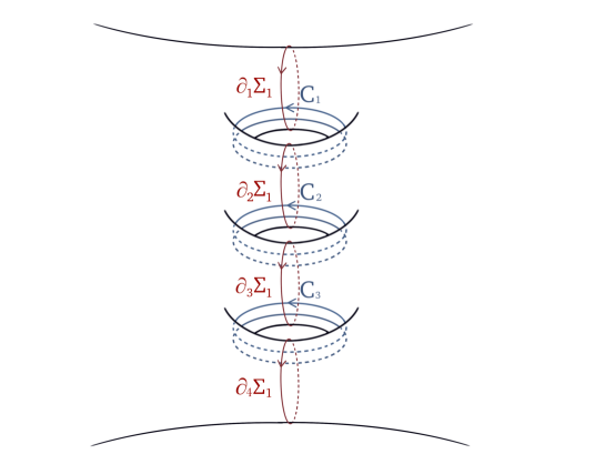
Figure 4.1. The one-forms $df_{k}$

The strips defining $df_{k}$, $k=1,2,3$ are the horizontal strips and the boundary curves are the vertical curves. Since $H_{C_{k}}$ and $df_{k}$ are in the same cohomology class, we have (by taking analytic limiting curves approaching $\partial_{m}\Sigma_{1}$)

$$\int_{\partial_{m}\Sigma_{1}}H_{C_{k}}=\int_{\partial_{m}\Sigma_{1}}df_{k}.$$

Here we let $k=1,\ldots,n-1$ where $n$ is the number of boundary curves (in Figure 4.1 we have $n=4$).

We see that

(4.22) $$\int_{\partial_{1}\Sigma_{1}}H_{C_{k}} =\left\{\begin{array}[]{ll}-1&k=1\\ 0&\text{otherwise}\end{array}\right.$$

(4.26) $$\int_{\partial_{2}\Sigma_{1}}H_{C_{k}} =\left\{\begin{array}[]{ll}1&k=1\\ -1&k=2\\ 0&\text{otherwise}\end{array}\right.$$

(4.27) $$\vdots \ \ \ \ \ \ \ \vdots$$

(4.31) $$\int_{\partial_{n-1}\Sigma_{1}}H_{C_{k}} =\left\{\begin{array}[]{ll}1&k={n-2}\\ -1&k=n-1\\ 0&\text{otherwise}\end{array}\right.$$

(4.34) $$\int_{\partial_{n}\Sigma_{1}}H_{C_{k}} =\left\{\begin{array}[]{ll}1&k={n-1}\\ 0&\text{otherwise}\end{array}\right.$$

Furthermore, the integral around any $C_{k}$ or internal homology curve is zero.

Remark 4.32.

The reason for the differing first and last integrals is that we haven’t included the redundant $H_{C_{n}}$ which corresponds to a curve traversing the outside of the entire surface.

We have the following result:

Theorem 4.33.

Assume that $\Sigma_{1}$ and $\Sigma_{2}$ are connected. Then

$$\mathcal{A}_{\mathrm{harm}}^{\mathrm{pe}}(\mathscr{R})=\{\mathbf{S}_{1}\partial\omega+\overline{\mathbf{S}}_{1}\overline{\partial}\omega:d\omega\in{\mathcal{A}_{\mathrm{harm}}(\Sigma_{1})}\}.$$

Proof.

The fact that $\mathbf{S}_{1}\partial\omega+\overline{\mathbf{S}}_{1}\overline{\partial}\omega$ is piecewise exact for $d\omega\in\mathcal{A}_{\mathrm{hm}}(\Sigma_{1})$ follows from Theorem 4.8. We need to show that such forms span the space.

To do so we first need an identity. Let $\omega_{k}$ be the harmonic function which is one on the $k$th boundary curve and zero on the remaining boundary curves. Set

$$\beta_{k}=\mathbf{S}_{1}\partial\omega_{k}+\overline{\mathbf{S}}_{1}\overline{\partial}\omega_{k}$$

We then have that by definition of $H_{C_{j}}$

$$\int_{C_{j}}\beta_{k} =(\beta_{k},\ast H_{C_{j}})_{\mathscr{R}}$$

$$=(\mathbf{S}^{\mathrm{h}}_{1}d\omega,\ast H_{C_{j}})_{\mathscr{R}}$$

$$=(d\omega,\mathbf{R}_{1}^{\mathrm{h}}\ast H_{C_{j}})_{\Sigma_{1}}$$

$$=\left(d\omega,\mathbf{R}_{1}^{\mathrm{h}}\left[\frac{1}{2}\left(\ast H_{C_{j}}-iH_{C_{j}}\right)+\frac{1}{2}\left(\ast H_{C_{j}}+iH_{C_{j}}\right)\right]\right)_{\Sigma_{1}}.$$

So

$$\int_{C_{j}}\beta_{k} =\left(\partial\omega_{k},\frac{1}{2}\mathbf{R}_{1}\left(\ast H_{C_{j}}-iH_{C_{j}}\right)\right)_{\Sigma_{1}}+\left(\,\overline{\partial}\omega_{k},\frac{1}{2}\overline{\mathbf{R}_{1}}\left(\ast H_{C_{j}}+iH_{C_{j}}\right)\right)_{\Sigma_{1}}$$

$$=\left(d\omega_{k},\frac{1}{2}\mathbf{R}_{1}\left(\ast H_{C_{j}}-iH_{C_{j}}\right)\right)_{\Sigma_{1}}+\left(\,d\omega_{k},\frac{1}{2}\overline{\mathbf{R}_{1}}\left(\ast H_{C_{j}}+iH_{C_{j}}\right)\right)_{\Sigma_{1}}$$

$$=\left(d\omega_{k},\mathbf{R}^{\mathrm{h}}_{1}\ast H_{C_{j}}\right)_{\Sigma_{1}}.$$

So we have

$$\int_{C_{j}}\beta_{k} =-\iint_{\Sigma_{1}}d\omega_{k}\wedge H_{C_{j}}$$

$$=-\int_{\partial\Sigma_{1}}\omega_{k}H_{C_{j}}$$

(4.35) $$=-\int_{\partial_{k}\Sigma_{1}}H_{C_{j}}.$$

It now follows immediately from (4.22) that the $\beta_{k}$ span $\mathcal{A}^{\mathrm{pe}}_{\mathrm{harm}}(\mathscr{R})$. This completes the proof. ∎

We also have the following elementary fact.

Proposition 4.34.

Fix a bordered Riemann surface $\Sigma$ of type $(g,n)$. Fix a subcollection $\gamma_{1},\ldots,\gamma_{m}$ of the boundary curves $\{\partial_{1}\Sigma,\ldots,\partial_{n}\Sigma\}$. For any $c_{1},\ldots,c_{m}\in\mathbb{C}$, there is an $\omega\in\mathcal{A}_{\mathrm{hm}}(\Sigma)$ whose boundary values are only non-zero on $\gamma_{1},\ldots,\gamma_{m}$ such that

$$\int_{\gamma_{k}}\omega=c_{k}.$$

Proof.

Let $j_{1},\ldots,j_{m}$ be the indices of the subcollection of curves; that is, $\gamma_{l}=\partial_{j_{l}}\Sigma$ for $l=1,\ldots,m$. Following a similar strategy as in the proof of Corollary 2.36, it is readily seen that we need to prove the existence of a solution to the system of equations

$$c_{k}=\int_{\gamma_{k}}\sum_{l=1}^{n}a_{l}\ast d\omega_{j_{l}}=\sum_{l=1}^{n}\int_{\partial_{j_{k}}\Sigma}a_{l}\ast d\omega_{j_{l}}=\sum_{l=1}^{n}\Pi_{j_{k}j_{l}}a_{l}.$$

This follows from the fact that any square submatrix of a positive-definite matrix is also positive-definite. ∎

Now we define a subclass of the harmonic measures which lie in the kernel of $\mathbf{T}_{1,2}$.

Definition 4.35.

We say that $\omega\in\mathcal{D}_{\text{harm}}(\Sigma_{1})$ is bridgeworthy if

1. it is constant on each boundary curve;

2. on any pair of boundary curves $\partial_{k}\Sigma_{1}$ and $\partial_{m}\Sigma_{1}$ that bound the same connected component of $\Sigma_{2}$, the boundary values of $\omega$ are equal.

We say that $\alpha\in\mathcal{A}_{\mathrm{hm}}(\Sigma_{1})$ is bridgeworthy if $\alpha=d\omega$ for some bridgeworthy harmonic function $\omega$. Denote the collection of bridgeworthy harmonic functions by $\lx@glossaries@gls@link{main}{Dbw}{\leavevmode\mathcal{D}_{\mathrm{bw}}}(\Sigma_{1})$, and the collection of bridgeworthy harmonic one-forms by $\lx@glossaries@gls@link{main}{Abw}{\leavevmode\mathcal{A}_{\mathrm{bw}}}(\Sigma_{1})$. The same definitions apply to $\Sigma_{2}$.

The name is meant to invoke the following geometric picture: $\omega$ is bridgeworthy if it has the same constant value on any pair of boundary curves which are connected by a “bridge” in $\Sigma_{2}$.

Remark 4.36.

If $\Sigma_{1}$ has more than one connected component, then a bridgeworthy harmonic one-form has anti-derivatives which are not bridgeworthy. This is because one can add to a bridgeworthy harmonic function $\omega$ any function which is constant on connected components without changing $d\omega$.

We will also need the following characterization of the kernel of $\mathbf{S}_{k}^{\mathrm{h}}$.

Proposition 4.37.

Assume that either $\Sigma_{1}$ or $\Sigma_{2}$ is connected. Fix $k=1$ or $k=2$. Let $d\omega_{k}\in\mathcal{A}_{\mathrm{hm}}(\Sigma_{k})$. The following are equivalent.

1. $\overline{\partial}\omega_{k}\in\overline{\partial}\mathcal{D}_{\mathrm{bw}}(\Sigma_{k})$.

2. $\partial\omega_{k}\in\partial\mathcal{D}_{\mathrm{bw}}(\Sigma_{k})$.

3. $\mathbf{S}_{k}^{\mathrm{h}}d\omega_{k}=0$.

4. $d\omega_{k}\in\mathcal{A}_{\mathrm{bw}}(\Sigma_{k})$.

Proof.

We assume throughout that $k=1$. It is then necessary and sufficient to show the equivalence for both the cases that $\Sigma_{1}$ is connected and that $\Sigma_{2}$ is connected. The case $k=2$ is obtained by symmetry.

We first show that (1) implies (3); assume that (1) holds. If $\Sigma_{2}$ is connected, then $\omega_{1}$ is constant, so $d\omega_{1}=0$ and (3) follows trivially. Now assume that $\Sigma_{1}$ is connected. Let $H\in\mathcal{D}_{\mathrm{bw}}(\Sigma_{1})$ be such that $\overline{\partial}H=\overline{\partial}\omega_{1}$. Then $\mathbf{O}_{1,2}H$ is constant on connected components of $\Sigma_{2}$, so by Theorem 4.16, $\dot{\mathbf{J}}_{1,2}H=-\dot{\mathbf{J}}_{2,2}\dot{\mathbf{O}}_{1,2}\dot{H}$ =0. So by Theorem 4.8

$$\mathbf{T}_{1,2}\overline{\partial}H+\overline{\mathbf{R}}_{1}\overline{\mathbf{S}}_{1}\overline{\partial}H=d\dot{\mathbf{J}}_{1,2}\dot{H}=0.$$

Since the holomorphic and anti-holomorphic parts must both be zero, we have $\mathbf{T}_{1,2}\overline{\partial}\omega_{1}=0$ and $\overline{\mathbf{R}}_{1}\overline{\mathbf{S}}_{1}\overline{\partial}\omega_{1}=0$. The latter implies that $\overline{\mathbf{S}}_{1}\overline{\partial}\omega_{1}=0$ by analytic continuation. The former together with Corollary 4.31 to $\overline{\omega}_{1}$, implies that

$$\mathbf{R}_{1}\mathbf{S}_{1}\partial\omega_{1}=0.$$

Hence $\mathbf{S}_{1}\partial\omega_{1}=0$ and therefore $\mathbf{S}_{1}^{\mathrm{h}}d\omega_{1}=0$. This shows that (1) implies (3). A similar argument shows that (2) implies (3).

Now assume that (3) holds, and that $\Sigma_{2}$ is connected. We will show that both (1) and (2) hold. Since holomorphic and anti-holomorphic parts of $\mathbf{S}_{1}^{\mathrm{h}}d\omega_{1}$ are zero, we have $\mathbf{S}_{1}\partial\omega_{1}=0$ and $\overline{\mathbf{S}}_{1}\overline{\partial}\omega_{1}=0$. By Corollary 4.31, we also have that

$$\mathbf{T}_{1,2}\overline{\partial}\omega_{1}=0\ \ \ \text{and}\ \ \ \overline{\mathbf{T}}_{1,2}\partial\omega_{1}=0.$$

Here, to show the left equation, we have applied the equivalence of parts (1) and (3) of Corollary 4.31 directly; whereas to show the right equation, we applied the conjugates of the equivalence of parts (1) and (3) to $\overline{\omega_{1}}$ to see that

$$0=\overline{\mathbf{S}}_{1}\overline{\partial}\omega_{1}=\overline{\mathbf{S}_{1}\partial\overline{\omega_{1}}}\ \ \Rightarrow\ \ 0=\overline{\mathbf{T}_{1,2}\overline{\partial}\overline{\omega_{1}}}=\overline{\mathbf{T}}_{1,2}\partial\omega_{1}.$$

We thus have that

$$d\mathbf{J}^{q}_{1,2}\omega_{1}=\mathbf{T}_{1,2}\overline{\partial}\omega_{1}+\overline{\mathbf{R}}_{1}\overline{\mathbf{S}}_{1}\overline{\partial}\omega_{1}=0,$$

and so $\mathbf{J}^{q}_{1,2}\omega_{1}$ is constant on connected components of $\Sigma_{2}$. Hence $H=\mathbf{O}_{2,1}\mathbf{J}_{1,2}^{q}\omega_{1}$ is bridgeworthy. Applying Theorem 4.18 yields

$$\dot{\mathbf{J}}_{1,1}\dot{\omega}_{1}-\dot{H}=\dot{\omega}_{1},$$

from which we obtain

$$d\dot{\mathbf{J}}_{1,1}\dot{\omega}_{1}-d\dot{H}=d\dot{\omega}_{1}.$$

Now Theorems 4.8 and 4.30 yield that

$$d\dot{\mathbf{J}}_{1,1}\dot{\omega}_{1}=\partial\dot{\omega}_{1}+\mathbf{T}_{1,1}\overline{\partial}\dot{\omega}_{1}+\overline{\mathbf{R}}_{1}\overline{\mathbf{S}}_{1}\overline{\partial}\dot{\omega}_{1}=0,$$

and inserting this in the above equation we obtain that $\overline{\partial}\omega_{1}=-\overline{\partial}H$. This proves that (3) implies (1) in the case that $\Sigma_{2}$ is connected. A similar argument, using the fact that $\overline{\mathbf{J}}_{1,2}^{q}\omega_{1}$ is constant on connected components of $\Sigma_{2}$ shows that $\partial\omega_{1}=-\partial G$ where $G=\mathbf{O}_{2,1}\mathbf{J}_{1,2}^{q}\omega_{1}$, so (3) implies (2) in the case that $\Sigma_{2}$ is connected.

Now assume that $\Sigma_{1}$ is connected and that (3) holds. We will show that (4) holds. We have that $\mathbf{S}_{1}^{h}d\omega_{1}=0$. Then by Theorem 4.30 $\mathbf{S}_{2}^{h}d\mathbf{O}_{2,1}\omega_{1}=0$. Thus

$$\mathbf{S}_{2}\partial\mathbf{O}_{1,2}\omega_{1}=0\ \ \ \text{and}\ \ \ \overline{\mathbf{S}}_{2}\overline{\partial}\mathbf{O}_{1,2}\omega_{1}=0.$$

Applying Corollary 4.31 parts (1)–(3) and Theorem 4.8 we see that

$$d{\mathbf{J}}_{2,1}{\mathbf{O}}_{1,2}\omega_{1}=\mathbf{T}_{2,1}\overline{\partial}\mathbf{O}_{2,1}\omega_{1}+\overline{\mathbf{R}}_{1}\overline{\mathbf{S}}_{2}\overline{\partial}\mathbf{O}_{1,2}\omega_{1}=0.$$

Thus $\mathbf{J}_{2,1}\mathbf{O}_{1,2}$ is locally constant. Similarly

$$d\mathbf{J}_{2,2}\mathbf{O}_{1,2}\omega_{1}=\overline{\partial}\mathbf{O}_{1,2}\omega_{1}+\mathbf{T}_{2,2}\overline{\partial}\mathbf{O}_{1,2}\omega_{1}+\overline{\mathbf{R}}_{2}\overline{\mathbf{S}}_{2}\overline{\partial}\mathbf{O}_{1.2}\omega_{1}=0$$

so $\mathbf{J}_{2,2}\mathbf{O}_{1,2}\omega$ is constant. Thus by Theorem 4.18 part (2) we see that

$$0=-\dot{\mathbf{O}}_{1,2}\dot{\mathbf{J}}_{2,1}\dot{\mathbf{O}}_{1,2}\dot{\omega}_{1}+\dot{\mathbf{J}}_{2,2}\dot{\mathbf{O}}_{1,2}\dot{\omega}_{1}=\dot{\mathbf{O}}_{1,2}\dot{\omega}_{1}.$$

Thus $\mathbf{O}_{1,2}\omega$ is constant, that is, $\omega_{1}$ is bridgeworthy. Thus (3) implies (4) in the case that $\Sigma_{1}$ is connected. It is obvious that (4) implies (1) and (4) implies (2) independently of the connectivity assumption.

In summary, we have shown the equivalence of (1), (2), and (3), and furthermore that (4) implies (1) and (2). It remains to show that (1) implies (4). Assuming that (1) holds, we have that $\omega_{1}=\tilde{\omega_{1}}+h$ where $\tilde{\omega_{1}}$ is bridgeworthy and $h$ is holomorphic on $\Sigma_{1}$. So $h=\omega_{1}-\tilde{\omega_{1}}$ has constant boundary values on $\partial\Sigma_{1}$. Fix a connected component $\Sigma_{1}^{0}$ and treat it as a subset of its double, so that the boundary is an analytic curve. We have that by Schwarz reflection $h$ extends to a holomorphic function on a neighbourhood of $\partial\Sigma_{1}^{0}$. Since $h$ is constant on the boundary it is constant on $\Sigma_{1}^{0}$. We have shown that $\omega_{1}=\tilde{\omega_{1}}+c$ where $c$ is constant on connected components and $\tilde{\omega_{1}}$ is bridgeworthy; thus $d\omega_{1}=d\tilde{\omega_{1}}\in\mathcal{A}_{\mathrm{b}w}(\Sigma_{1})$. ∎

5. Dirichlet problem for $L^{2}$ harmonic one-forms

5.1. Assumptions throughout this section

In this section, we consider a Riemann surface $\Sigma$ of type $(g,n)$.

5.2. About this section

In this section, we give a complete theory and solution of the Dirichlet problem for $L^{2}$ one-forms. This includes developing a theory of their boundary values, which we show can be identified with the Sobolev space $H^{-1/2}(\partial\Sigma)$. Given an element of $H^{-1/2}(\partial\Sigma)$ together with sufficient cohomological data, there is a unique $L^{2}$ harmonic one-form on $\Sigma$ with those boundary values. Furthermore, the solution depends continuously on the data.

We also characterize the boundary values in terms of equivalence classes of $L^{2}$ harmonic one-forms defined in collar neighbourhoods. We show that there is a one-to-one correspondence between elements of $H^{-1/2}$ and such equivalence classes, and this allows us to use the theory of CNT boundary values developed in Section 3 to solve the problem. Anti-derivatives of such forms have well-defined CNT boundary values, which can be identified with elements of $H^{1/2}$ (after removing a period). This reflects the fact that $H^{-1/2}$ is in some sense the set of distributional derivatives of elements of $H^{1/2}$.

We outline the approach. In Section 5.3 we give the routine solution to the Dirichlet problem for smooth boundary values. This section does not contain any original material, but rather serves to outline how the cohomological data is dealt with without the distraction of analytic complications. In particular it establishes the cohomological preliminaries used in the proof of the general case. In Section 5.4, we show the equivalence between the CNT and $H^{-1/2}$ boundary values of one-forms. The bulk of the main results, namely the proof of the well-posedness of the Dirichlet problem for CNT boundary values, is given in Section 5.5. Finally, in Section 5.6 we use the equivalence between $H^{-1/2}$ and CNT boundary values of one-forms, together with the solution to the CNT boundary value problem given in Section 5.5, to solve the $H^{-1/2}$ Dirichlet problem for $L^{2}$ one-forms.

5.3. Formulation of the regular Dirichlet problem

Let $\Sigma$ be a Riemann surface of type $(g,n)$. We describe a network of smooth curves on $\Sigma$. By Corollary 2.46 we can treat $\Sigma$ as a subset of a compact Riemann surface $\mathscr{R}$ obtained by either sewing on caps, or as a subset of the double. In the latter case, the boundary curves are analytic, and in the former, the boundary curves can be taken to be analytic, if one sews on caps via analytic parametrizations.

For the moment, let $\gamma_{1},\ldots,\gamma_{2g}$ be specific simple smooth closed curves which are generators of the homology of the surface $\mathscr{R}$ obtained by sewing on caps. We choose these curves such that they lie in $\Sigma$, and furthermore, such that when $\mathscr{R}$ is cut along these curves we obtain a polygonal decomposition of $\mathscr{R}$ in the standard way. Denote by $c_{k}$ curves which are isotopic to the boundaries $\partial_{k}\Sigma$ for $k=1,\ldots,n$; we assume that these are non-intersecting. See Figure 5.1 for a picture of the polygonal decomposition.

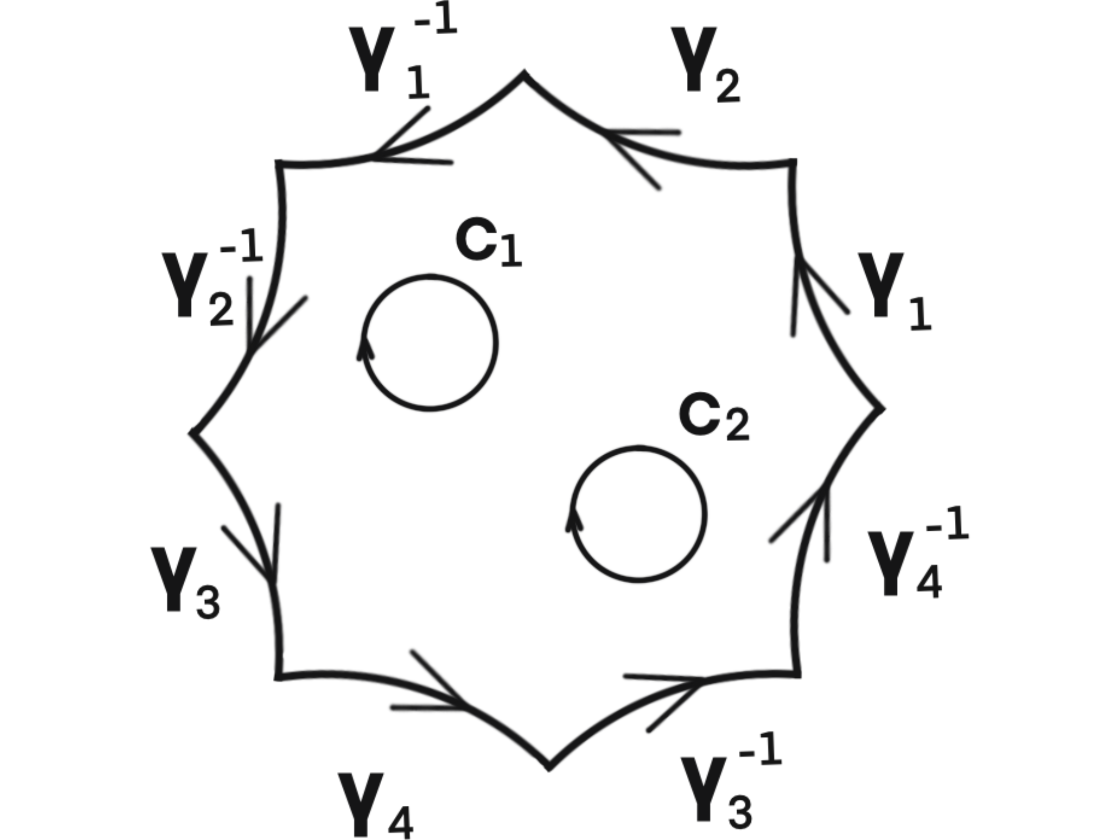
Figure 5.1. Polygononal decomposition of the bordered surface

For any $\alpha\in\mathcal{A}_{\mathrm{harm}}(\Sigma)$, we have that $\int_{\gamma}\alpha$ depends only on the homotopy class of $\gamma$, so we can define

$$\int_{\partial_{k}\Sigma}\alpha=\int_{c_{k}}\alpha,$$

and with this definition, it is clear that if we let $\gamma$ denote the boundary of the polygon then

(5.1) $$\sum_{k=1}^{n}\int_{\partial_{k}\Sigma}\alpha=-\int_{\gamma}\alpha=0$$

for any $\alpha\in\mathcal{A}_{\mathrm{harm}}(\Sigma)$.

We also need the following facts regarding the double $\Sigma^{d}$ of $\Sigma$. There is a basis of generators $\{\Gamma_{1},\ldots,\Gamma_{4g+2n-2}\}$ for the homology of $\Sigma^{d}$ so that $\Gamma_{k}=\gamma_{k}$ for $k=1,\ldots,2g$ and $\Gamma_{k}=\partial_{k}\Sigma$ for $k=2g+2,\ldots,2g+n-1$.

Now let $\{\varepsilon_{1},\ldots,\varepsilon_{4g+2n-2}\}$ be a dual basis of closed one-forms on $\Sigma^{d}$. By the Hodge decomposition theorem these can be chosen to be harmonic. We thus have

(5.2) $$\int_{\Gamma_{k}}\varepsilon_{j}=\delta_{j}^{k},\ \ \ \ j,k=1,\ldots,4g+2n-2$$

where $\delta_{j}^{k}$ is the Kronecker delta.

Our data in the Dirichlet problem will consist of continuous one-forms on the boundary curves together with specified period information. Since $\Sigma$ is a bordered surface, the notion of continuous or smooth one-forms is well-defined; explicitly, $\alpha$ is a continuous or smooth one-form if for some collar chart $\phi$ of $\partial_{k}\Sigma$, setting $\psi=\left.\phi\right|_{\partial_{k}\Sigma}$ its expression in coordinates is $\psi^{*}\alpha=h(e^{i\theta})\,d\theta$ for some continuous or smooth function $h$ (see Remark 2.15).

The $\mathcal{C}^{\infty}$ Dirichlet problem for one-forms is as follows. Let $\Sigma$ be a Riemann surface of type $(g,n)$. We refer to the following data as smooth Dirichlet data for forms on a Riemann surface:

1. $\mathcal{C}^{\infty}$ one-forms $\beta_{k}$ on $\partial_{k}\Sigma$ for each $k=1,\ldots,n$, satisfying

   $$\int_{\partial_{1}\Sigma}\beta_{1}+\cdots+\int_{\partial_{n}\Sigma}\beta_{n}=0;$$

2. constants $\rho_{1},\ldots,\rho_{n}\in\mathbb{C}$ satisfying

   $$\rho_{1}+\cdots+\rho_{n}=0;$$

   and

3. constants $\sigma_{1},\ldots,\sigma_{2g}\in\mathbb{C}$.

Definition 5.1.

We say that a harmonic one-form $\alpha$ on $\Sigma$ solves the Dirichlet problem with data $(\beta,\rho,\sigma)$ if $\alpha$ extends smoothly to $\partial\Sigma$ and

1. for any tangent vector $v_{p}$ to $\partial_{k}\Sigma$ at any point $p\in\partial_{k}\Sigma$, $\alpha(v_{p})=\beta_{k}(v_{p})$;

2. for all $k=1,\ldots,n$

   $$\int_{\partial_{k}\Sigma}\ast\alpha=\rho_{k};$$

   and

3. for all $k=1,\ldots,2g$

   $$\int_{\gamma_{k}}\alpha=\sigma_{k}.$$

Note that the one-forms $\beta_{k}$ specify the periods around the boundary curves $\partial_{k}\Sigma$. Condition (2) is motivated as follows. For any harmonic measure $\sum_{k}d\omega_{k}$ and any solution $\alpha$, the form $\alpha+\sum_{k}d\omega_{k}$ still satisfies (1) and (3), because $\sum_{k}d\omega_{k}$ is exact and $\sum_{k}d\omega_{k}=0$ along $\partial\Sigma$. In fact, this is the only indeterminacy and the condition (2) uniquely determines the solution.

It is elementary that a solution exists; in fact, the smooth Dirichlet problem for one-forms is essentially a smooth Dirichlet problem for functions. One simply subtracts off forms whose periods match the data, so that one obtains boundary values of exact forms. One then solves the Dirichlet problem for functions with respect to the primitive on the boundary. The solution to the problem for functions is well-known:

Theorem 5.2.

Let $X$ be a compact Riemannian manifold with boundary $\partial X,$ and $\Delta$ is the Laplacian on $X$. Then the Dirichlet problem

(5.3) $$\begin{cases}\Delta u=0\\ u|_{\partial X}=f\in\mathcal{C}^{\infty}(\partial X)\end{cases}$$

has a unique solution $u\in\mathcal{C}^{\infty}(X)$.

For the proof see e.g. [Hormander] page 264 Example 1.

Theorem 5.3.

For smooth Dirichlet data $(\beta,\rho,\sigma)$ there exists an $\alpha\in\mathcal{C}^{\infty}(\mathrm{cl}(\,\Sigma))$ which solves the smooth Dirichlet problem.

Proof.

We assume that $\Sigma$ is included in its double, so that the boundary curves are analytic. Setting

$$\lambda_{k}=\int_{\partial_{k}\Sigma}\beta_{k}$$

for $k=1,\ldots,n$, by Corollary 2.36 there is a $\mu\in\ast\mathcal{A}_{\mathrm{hm}}$ such that

(5.4) $$\int_{\partial_{k}\Sigma}\mu=\lambda_{k}$$

for every $k$ and a harmonic one-form $\eta$ in the span of $\{\varepsilon_{1},\ldots,\varepsilon_{2g}\}$, which were defined in connection to (5.2), such that

$$\int_{\gamma_{j}}\eta=\sigma_{j}-\int_{\gamma_{j}}\mu$$

for $j=1,\ldots,2g$. Since $\partial_{k}\Sigma$ is null-homotopic in $\mathscr{R}$, we have

(5.5) $$\int_{\partial_{k}\Sigma}\eta=0$$

for $k=1,\ldots,n$. Observe that the one-forms $\eta$ and $\mu$ are smooth on $\partial\Sigma$.

Define functions $h_{k}$ on the boundary curves $\partial_{k}\Sigma$ as follows. Each $h_{k}$ is the anti-derivative of $\beta_{k}-\mu-\eta$ on $c_{k}$, that is, for any tangent vector $v$ to the boundary $c_{k}$

$$dh_{k}(v)=\beta_{k}(v)-\mu(v)-\eta(v).$$

Note that each anti-derivative is single-valued by (5.3) and the definition of $\varepsilon_{k}$. By Theorem 2.35 we can add a suitable harmonic measure $d\omega\in\mathcal{A}_{\mathrm{hm}}(\Sigma)$ (which is exact and does not change the periods) in order to ensure that condition (2) in Definition 5.1 is satisfied. Solving now the ordinary Dirichlet problem with smooth data $h_{1},\ldots,h_{n}$ on the boundary curves using Theorem 5.3, we obtain a smooth $h\in\mathcal{D}_{\mathrm{harm}}(\Sigma)$. Then

$$\alpha=dh+\mu+\eta$$

is the desired solution to the problem. It is not hard to show that the solution is unique by keeping track of the periods and using uniqueness in Theorem 5.3. ∎

5.4. Boundary values of $L^{2}$ forms and $H^{-1/2}$

In this section, we will show that $H^{-1/2}(\partial_{k}\Sigma)$ of a boundary curve $\partial_{k}\Sigma$ can be identified with an equivalence class of harmonic one-forms defined in a collar neighbourhood. The idea is fairly simple, and we give a sketch in the case of the circle $\mathbb{S}^{1}$ before launching into the details. We can think of smooth one-forms $h(\theta)d\theta$ on the circle as dual to functions on the circle via the pairing

$$L_{hd\theta}(f)=\int_{\mathbb{S}^{1}}f\cdot hd\theta.$$

Of course if $hd\theta$ is in $H^{-1/2}(\mathbb{S}^{1})$ and $f\in H^{1/2}(\mathbb{S}^{1})$, then this only makes sense distributionally.

On the other hand, given an $\alpha\in\mathcal{A}_{\mathrm{harm}}(\mathbb{A}_{r,1})$ for an annulus $\mathbb{A}_{r,1}$, by the First Anchor Lemma 3.14 one can define a pairing

(5.6) $$\lim_{r\nearrow 1}\int_{|z|=r}f\alpha.$$

If $\alpha$ were smooth, we could identify this integral with

$$\int_{\mathbb{S}^{1}}f\alpha.$$

In the general case that $f$ is in $H^{1/2}(\mathbb{S}^{1})$, it turns out that the pairing makes sense, and in fact all elements of $H^{-1/2}(\mathbb{S}^{1})$ can be represented this way. The same idea works for the border of a Riemann surface, provided that we treat it as an analytic curve (see Remark 2.30).

The remainder of this section is dedicated to filling in the details of this sketch. The payoff of this approach is that it makes it possible to use the machinery of CNT boundary values to solve the Dirichlet problem for one-forms with $H^{-1/2}$ boundary data. In this way one obtains a complete theory of the boundary values of $L^{2}$ harmonic one-forms for bordered surfaces.

We begin by defining an equivalence relation, such that the equivalence classes represent the boundary values of the one-form. Later we will see that each equivalence class can be identified with a unique element of $H^{-1/2}$, and vice-versa.

Definition 5.4 (Equivalence relation for CNT Dirichlet boundary values of one-forms).

For collar neighbourhoods $A$ and $B$ of $\partial_{k}\Sigma$, let $\alpha\in\mathcal{A}_{\mathrm{harm}}(A)$ and $\beta\in\mathcal{A}_{\mathrm{harm}}(B)$. We say that $\alpha\sim\beta$ if

1. there is a collar neighbourhood $U_{k}\subseteq A\cap B$ of $\partial_{k}\Sigma$ and a $\delta\in\mathcal{A}_{\mathrm{harm}}(U_{k})$ such that $\alpha-\delta,\beta-\delta\in\mathcal{A}^{\mathrm{e}}_{\mathrm{harm}}(U_{k})$;

2. if $f,g\in\mathcal{D}_{\mathrm{harm}}(U_{k})$ are such that $df=\alpha-\delta$ and $dg=\beta-\delta$, then the CNT boundary values of $f-g$ are constant on $\partial_{k}\Sigma$ up to a null set.

In brief, $\alpha$ and $\beta$ are equivalent if their multi-valued primitives agree on the boundary up to integration constant. When the boundary curve is not clear from context, we will say “$\alpha\sim\beta$ on $\partial_{k}\Sigma$”.

It turns out that if $\alpha\sim\beta$ via some $\delta$, then any one-form $\delta^{\prime}\in\mathcal{A}_{\mathrm{harm}}(U^{\prime})$ satisfying (1) also satisfies (2). To see this, choose a collar neighbourhood $V\subset U\cap U^{\prime}$, which exists by Proposition 2.16. Observe that $\delta^{\prime}-\delta=(\alpha-\delta)-(\alpha-\delta^{\prime})$ has a primitive $h$ on $V$. So if $f$ and $g$ are the primitives of $\alpha-\delta$ and $\beta-\delta$ respectively, then $f-h$ and $g-h$ are the unique primitives of $\alpha-\delta^{\prime}$ and $\beta-\delta^{\prime}$ up to constants. But $(f-h)-(g-h)=f-g$ has constant CNT boundary values on $\partial_{k}\Sigma$ up to a null set, which proves the claim. With this fact in hand, it is not hard to verify that $\sim$ is an equivalence relation.

Definition 5.5.

[CNT Dirichlet boundary values for one-forms] Let $\mathcal{U}_{k}$ denote the collection of collar neighbourhoods of $\partial_{k}\Sigma$. Define

$$\lx@glossaries@gls@link{main}{Dbvaluescomp}{\leavevmode\mathcal{H}^{\prime}(\partial_{k}\Sigma)}=\{\alpha\in\mathcal{A}_{\mathrm{harm}}(U_{k});\,U_{k}\in\mathcal{U}_{k}\}/\sim.$$

We also denote

$$\lx@glossaries@gls@link{main}{Dbvalues}{\leavevmode\mathcal{H}^{\prime}(\partial\Sigma)}=\{([\alpha_{1}],\ldots,[\alpha_{n}]);\,\alpha_{k}\in\mathcal{H}^{\prime}(\partial_{k}\Sigma)\}.$$

If $\alpha\in\mathcal{A}_{\mathrm{harm}}(U)$ where $U$ contains a collar neighbourhood $U_{k}$ of each boundary, then we set

$$[\alpha]:=([\alpha_{1}],\ldots,[\alpha_{n}]),$$

where $\alpha_{k}=\left.\alpha\right|_{U_{k}}$.

For fixed $k$, any equivalence class $[\beta]\in\mathcal{H}^{\prime}(\partial_{k}\Sigma)$ has a well-defined boundary period. Given a representative $\beta\in\mathcal{A}_{\mathrm{harm}}(U_{k})$ for some collar neighbourhood $U_{k}$, let $c_{k}$ be a smooth closed curve in $U_{k}$ which is homotopic to $\partial_{k}\Sigma$, and define

$$\int_{\partial_{k}\Sigma}[\beta]=\int_{c_{k}}\beta.$$

To see that this is well-defined, let $\beta^{\prime}\in\mathcal{A}_{\mathrm{harm}}(U_{k}^{\prime})$ be another representative of $[\beta]$ and $c_{k}^{\prime}$ be another such curve. By Proposition 2.16 there is a canonical collar chart $\phi_{k,r}:U_{k,r}\rightarrow\mathbb{A}_{r,1}$ such that the inner boundary $\Gamma$ of $U_{k,r}$ is contained in $U_{k}\cap U_{k}^{\prime}$ and $\phi_{k,r}$ extends analytically to $\Gamma$. Since $\Gamma$ is isotopic to $\partial_{k}\Sigma$, it is isotopic to $c_{k}$ in $U_{k}$ and isotopic to $c_{k}^{\prime}$ in $U_{k}^{\prime}$. Thus

$$\int_{c_{k}^{\prime}}\beta^{\prime}=\int_{\Gamma}\beta=\int_{c_{k}}\beta,$$

proving the claim.

It also follows directly from the definition of the equivalence classes that $\mathcal{H}^{\prime}(\partial\Sigma)$ is conformally invariant in the following sense.

Proposition 5.6.

Let $\Sigma_{1}$ and $\Sigma_{2}$ be bordered surfaces and fix borders $\partial_{k_{1}}\Sigma_{1}$ and $\partial_{k_{2}}\Sigma_{2}$ which are homeomorphic to $\mathbb{S}^{1}$. Let $U$ and $V$ be collar neighbourhoods of $\partial_{k_{1}}\Sigma_{1}$ and $\partial_{k_{2}}\Sigma_{2}$ respectively, and let $f:U\rightarrow V$ be a conformal map. Then for any two representatives $\alpha$ and $\beta$ of $[\alpha]\in\mathcal{H}^{\prime}(\partial_{k_{2}}\Sigma_{2})$ we have

$$[f^{*}\alpha]=[f^{*}\beta].$$

In particular, we have a well-defined pull-back map

$$f^{*}:\mathcal{H}^{\prime}(\partial_{k_{2}}\Sigma_{2}) \rightarrow\mathcal{H}^{\prime}(\partial_{k_{1}}\Sigma_{1})$$

$$[\alpha] \mapsto[f^{*}\alpha].$$

We will require the following elementary lemma, in order to define a norm on $\mathcal{H}^{\prime}(\partial_{k}\Sigma)$.

Lemma 5.7.

Let $[\alpha]\in\mathcal{H}^{\prime}(\mathbb{S}^{1})$ treated as the border of a subset of the disk $\mathbb{D}$. Then $\alpha$ has a unique representative of the form

$$\alpha=f(z)dz+\overline{g(z)}d\bar{z}+\delta$$

where $f(z),g(z)\in\mathcal{D}(\mathbb{D})$ have the form

$$f(z)=\sum_{n=2}^{\infty}f_{n}\,z^{n},\ \ \ \overline{g(z)}=\sum_{n=2}^{\infty}\overline{g_{n}}\,\overline{z}^{n},$$

and

$$\delta=\frac{a}{4\pi i}\left(\frac{dz}{z}-\frac{d\overline{z}}{\overline{z}}\right).$$

for some constant $a\in\mathbb{C}$

Proof.

This follows easily from the definition of $\mathcal{H}^{\prime}(\Gamma)$ and the existence of solutions to the Dirichlet problem on the disk, after observing that

$$b\left(\frac{dz}{z}+\frac{d\bar{z}}{\bar{z}}\right)$$

is equivalent to $0$ in $\mathcal{H}^{\prime}(\mathbb{S}^{1})$ for any $b\in\mathbb{C}$. Uniqueness is obvious. ∎

This allows us to define a norm on $\mathcal{H}^{\prime}(\mathbb{S}^{1})$. Given any $[\alpha]$ let

$$\alpha=f(z)dz+\overline{g(z)}d\overline{z}+\frac{\lambda}{4\pi i}\left(\frac{dz}{z}-\frac{d\bar{z}}{\bar{z}}\right)$$

be the representative given by Lemma 5.7. We define

$$\|[\alpha]\|^{2}_{\mathcal{H}^{\prime}(\mathbb{S}^{1})}=\|f(z)dz+\overline{g(z)}d\bar{z}\|^{2}_{\mathcal{A}_{\mathrm{harm}}(\mathbb{D})}+|\lambda|^{2}.$$

For any boundary curve $\partial_{k}\Sigma$, we define a norm on $\mathcal{H}^{\prime}(\partial_{k}\Sigma)$ as follows. Choose a collar chart $\phi:U\rightarrow\mathbb{A}_{r,1}$ of $\partial_{k}\Sigma$. Implicitly using Proposition 5.6, we define

(5.7) $$\|[\alpha]\|_{\mathcal{H}^{\prime}(\partial_{k}\Sigma)}=\|\phi^{*}[\alpha]\|_{\mathcal{H}^{\prime}(\mathbb{S}^{1})}.$$

This norm of course depends on the collar chart. However, we will see ahead that different collar charts induce equivalent norms.

Given a collection $\phi=(\phi_{1},\ldots,\phi_{n})$ of collar charts of $\partial_{1}\Sigma,\ldots,\partial_{n}\Sigma$, we define a norm on $\mathcal{H}^{\prime}(\partial\Sigma)$ by

(5.8) $$\|([\alpha_{1}],\ldots,[\alpha_{n}])\|^{2}_{\mathcal{H}^{\prime}(\partial\Sigma)}=\|[\alpha_{1}]\|^{2}_{\mathcal{H}^{\prime}(\partial_{1}\Sigma)}+\cdots\|[\alpha_{n}]\|^{2}_{\mathcal{H}^{\prime}(\partial_{n}\Sigma)}.$$

Again, this norm depends on the collection of collar charts $\phi$.

Regarding the norm defined above, we state the following lemma which will be useful in connection to Theorem 5.11 and Lemma 5.19 ahead.

Lemma 5.8.

Let $\phi:U\rightarrow\mathbb{A}_{r,1}$ be a collar chart defined near $\partial_{k}\Sigma$ for fixed $k$. Then

$$h\mapsto h\circ\phi$$

is a bounded isomorphism from $H^{1/2}(\mathbb{S}^{1})$ to $H^{1/2}(\partial_{k}\Sigma)$.

Proof.

By Carathéodory’s theorem and the Schwarz reflection principle, $\phi$ extends to a conformal map from a doubly connected neighbourhood $V$ of $\partial_{k}\Sigma$ to the annulus $\mathbb{A}_{r,1/r}$. The restriction of $\phi$ to $\partial_{k}\Sigma$ is thus an analytic diffeomorphism between the compact manifolds $\partial_{k}\Sigma$ and $\mathbb{S}^{1}$, from which and Lemma 2.26 the claim follows. ∎

Lemma 5.9.

Let $\varphi:C_{1}\to C_{2}$ be a quasisymmetric mapping between the closed smooth curves $C_{j}$, $j=1,2$. Then $\varphi$ induces an equivalence between $\dot{H}^{\frac{1}{2}}(C_{1})$ and $\dot{H}^{\frac{1}{2}}(C_{2})$, i.e.

$$\|f\|_{\dot{H}^{\frac{1}{2}}(C_{2})}\approx\|f\circ\varphi\|_{\dot{H}^{\frac{1}{2}}(C_{1})}.$$

As a consequence, we have that if $\phi_{k}$ is a quasisymmetric map from $\mathbb{S}^{1}\to\partial_{k}\Sigma$ then

$$\|f\|_{\dot{H}^{\frac{1}{2}}(\partial_{k}\Sigma)}\approx\|f\circ\varphi_{k}\|_{\dot{H}^{\frac{1}{2}}(\mathbb{S}^{1})}.$$

Proof.

This is just a special case of Theorem 5.1 in [Koskela]. ∎

Let $\Sigma$ be a bordered Riemann surface of type $(g,n)$. Fixing $k$, we can define a pairing between elements of $H^{1/2}(\partial_{k}\Sigma)$ and $\mathcal{H}^{\prime}(\partial_{k}\Sigma)$ as follows. Given $[\alpha]\in\mathcal{H}^{\prime}(\partial_{k}\Sigma)$ and $h\in H^{1/2}(\partial_{k}\Sigma)$, let $\alpha\in\mathcal{A}(U)$ be a representative of $[\alpha]$ for a collar neighbourhood $U$ of $\partial_{k}\Sigma$, and let $H\in\mathcal{D}_{\mathrm{harm}}(U^{\prime})$ have CNT boundary values $h$. There exists at least one such $H$, by solving the Dirichlet problem on $\Sigma$ with $H=h$ on $\partial_{k}\Sigma$ and $0$ on the other boundary curves. By Proposition 2.16 we can choose a common collar neighbourhood $V\subset U\cap U^{\prime}$. Define

(5.9) $$L_{[\alpha]}(h)=\int_{\partial_{k}\Sigma}[H\alpha]=\lim_{\epsilon\searrow 0}\int_{\Gamma_{\epsilon}}H\alpha$$

for limiting curves $\Gamma_{\epsilon}$ approaching $\partial_{k}\Sigma$. We have already shown that for fixed $H$ this is well-defined. By the second anchor Lemma 3.15 for any two $H_{m}\in\mathcal{D}_{\mathrm{harm}}(U_{m})$ on collar neighbourhoods $U_{m}$ for $m=1,2$ with the same boundary values, we have for fixed $\alpha$

$$\int_{\partial_{k}\Sigma}H_{1}\alpha=\int_{\partial_{k}\Sigma}H_{2}\alpha.$$

Thus $L_{[\alpha]}$ is well-defined.

The pairing is invariant under pull-back.

Proposition 5.10.

Let $\Sigma_{1}$ and $\Sigma_{2}$ be bordered surfaces and fix borders $\partial_{k_{1}}\Sigma_{1}$ and $\partial_{k_{2}}\Sigma_{2}$ which are homeomorphic to $\mathbb{S}^{1}$. Let $U$ and $V$ be collar neighbourhoods of $\partial_{k_{1}}\Sigma_{1}$ and $\partial_{k_{2}}\Sigma_{2}$ respectively, and let $f:U\rightarrow V$ be a conformal map. For any $H\in H^{1/2}(\partial_{k_{2}}\Sigma_{2})$,

$$\int_{\partial_{k_{2}}\Sigma_{2}}[\alpha]H=\int_{\partial_{k_{1}}\Sigma_{1}}f^{*}[\alpha]\,H\circ f.$$

Proof.

Let $\phi:U_{2}\rightarrow\mathbb{A}_{r,1}$ be a collar chart of $\partial_{k_{2}}\Sigma_{2}$. Then $\phi\circ f:U_{1}\rightarrow\mathbb{A}_{r,1}$ is a collar chart of $\partial_{k_{1}}\Sigma$, shrinking $U_{2}$ if necessary. Let $\Gamma^{2}_{r}$ be the limiting curves $\phi^{-1}(|z|=r)$ induced by $\phi$, and similarly $\Gamma^{1}_{r}$ by $\phi\circ f$ (so that $f(\Gamma^{1}_{r})=\Gamma^{2}_{r})$.

Now choose a representative $\alpha$ of $[\alpha]$ and let $h$ be an extension of $H$ to a collar neighbourhood of $\partial_{k_{2}}\Sigma_{2}$. Then by the Anchor Lemmas 3.14 and 3.15 and a change of variables, we have

$$\int_{\partial_{k_{2}}\Sigma_{2}}[\alpha]H =\lim_{r\nearrow 1}\int_{\Gamma^{2}_{r}}\alpha h=\lim_{r\nearrow 1}\int_{\Gamma^{1}_{r}}f^{*}\alpha\,h\circ f$$

$$=\int_{\partial_{k_{1}}\Sigma_{1}}f^{*}[\alpha]H\circ f$$

where in the last equality we have also used Proposition 5.6. ∎

Theorem 5.11.

Let $\Sigma$ be a bordered Riemann surface of type $(g,n)$. For any fixed $k\in\{1,\ldots,n\}$, the bijection

$$\mathcal{H}^{\prime}(\partial_{k}\Sigma) \rightarrow H^{-1/2}(\partial_{k}\Sigma)$$

$$[\alpha] \mapsto L_{[\alpha]}$$

is a bounded isomorphism.

The proof of the theorem will require the following result.

Theorem 5.12.

Let $L$ be in $H^{-1/2}(\mathbb{S}^{1})$. Then there is an $\alpha\in\mathcal{A}_{\mathrm{harm}}(\mathbb{A}_{r,1})$ such that

(5.10) $$L(f)=\lim_{s\nearrow 1}\int_{|z|=s}f\alpha.$$

Proof.

Since $H^{1/2}(\mathbb{S}^{1})$ is a Hilbert space, Riesz representation theorem yields that there exists a unique $F\in H^{1/2}(\mathbb{S}^{1})$ such that, if $f=\sum_{n=-\infty}^{\infty}\hat{f}(n)e^{in\theta}$ and $F=\sum_{n=-\infty}^{\infty}\hat{F}(n)e^{in\theta}$ then

$$L(f)=\langle f,F\rangle_{H^{1/2}(\mathbb{S}^{1})}=\sum_{n=-\infty}^{\infty}\left(1+|n|^{2}\right)^{1/2}\hat{f}(n)\overline{\hat{F}(n)}.$$

Moreover $\|L\|_{H^{-1/2}(\mathbb{S}^{1})}=\|F\|_{H^{1/2}(\mathbb{S}^{1})}.$ Now by Parseval’s formula we also have

(5.11) $$\sum_{n=-\infty}^{\infty}\left(1+|n|^{2}\right)^{1/2}\hat{f}(n)\overline{\hat{F}(n)}=\frac{1}{2\pi}\int_{0}^{2\pi}f(e^{i\theta})((1-\partial^{2}_{\theta})^{1/2}F)(e^{i\theta})\,d\theta.$$

This and the requirement of harmonicity of $\alpha$ suggests that the desired $\alpha$ should be taken as the Poisson extension of $((1-\partial^{2}_{\theta})^{1/2}F)(e^{i\theta})$ (i.e. its convolution with the Poisson kernel of the unit disk), which for $s\leq 1$ yields that

(5.12) $$\alpha(se^{i\theta})=\sum_{n=-\infty}^{\infty}\left(1+|n|^{2}\right)^{1/2}\hat{F}(n)\,s^{|n|}\,e^{in\theta}.$$

Moreover, a calculation reveals that for $0<r<1$ one has

(5.13) $$\|\alpha\|^{2}_{L^{2}(\mathbb{A}_{r,1})}=\pi\sum_{n=-\infty}^{\infty}(1-r^{2|n|+2})\frac{1+|n|^{2}}{1+|n|}|\hat{F}(n)|^{2}\lesssim\sum_{n=-\infty}^{\infty}(1+|n|^{2})^{1/2}|\hat{F}(n)|^{2}<\infty$$

since $F\in H^{1/2}(\mathbb{S}^{1}).$ Therefore $\alpha\in\mathcal{A}_{\mathrm{harm}}(\mathbb{A}_{r,1})$, as desired. ∎

We now return to the proof of Theorem 5.11.

Proof of Theorem 5.11.

Let $\phi:U\rightarrow\mathbb{A}_{r,1}$ be a collar chart. For any $h\in H^{1/2}(\partial_{k}\Sigma)$, recall that we have

(5.14) $$\int_{\partial_{k}\Sigma}[\alpha]h=\int_{\mathbb{S}^{1}}\phi^{*}[\alpha]h\circ\phi$$

by Proposition 5.10. Thus, by Lemma 5.8 and recalling the definition (5.7) of the chart-dependent norm, it is enough to prove the claim on $\mathcal{H}^{\prime}(\mathbb{S}^{1})$.

We first need to show that for any given $[\alpha]\in\mathcal{H}^{\prime}(\mathbb{S}^{1})$, the linear functional $L_{[\alpha]}$ is bounded, and hence in $H^{-1/2}(\mathbb{S}^{1})$. To see this, let $\alpha$ be a representative as in Lemma 5.7, so that $\alpha-\delta$ is exact where

$$\delta=\frac{a}{4\pi i}\left(\frac{dz}{z}-\frac{d\bar{z}}{\bar{z}}\right)$$

for some $a\in\mathbb{C}$. Observe that

$$a=\int_{\mathbb{S}^{1}}[\alpha].$$

For any $h\in H^{1/2}(\mathbb{S}^{1})$ let $H$ be its unique harmonic extension in $\mathcal{D}_{\mathrm{harm}}(\mathbb{D})$, and write $H(z)=H_{1}(z)+H(0)$ where $H_{1}(0)=0$. Recall that

$$\|h\|^{2}_{\mathcal{H}^{1/2}(\mathbb{S}^{1})}=|H(0)|^{2}+\|dH\|^{2}_{\mathcal{D}_{\mathrm{harm}}(\mathbb{D})}.$$

By the mean-value theorem for the harmonic function $H_{1}$, one has

$$\lim_{r\nearrow 1}\int_{|z|=r}\alpha(z)H(z) =\lim_{r\nearrow 1}\int_{|z|=r}H(0)\alpha(z)+\lim_{r\nearrow 1}\int_{|z|=r}\alpha H_{1}(z)$$

$$=\lim_{r\nearrow 1}\int_{|z|=r}H(0)\delta(z)+\lim_{r\nearrow 1}\int_{|z|=r}(\alpha-\delta)H_{1}(z)$$

$$={{a}}H(0)-\iint_{\mathbb{D}}(\alpha-\delta)\wedge_{w}dH_{1}(z),$$

so the Cauchy-Schwarz inequality and Corollary 2.28 yield

$$\left|\lim_{r\nearrow 1}\int_{|z|=r}\alpha(z)H(z)\right| \leq|aH(0)|+\|\alpha-\delta\|_{\mathcal{A}_{\mathrm{harm}}(\mathbb{D})}\|H\|_{\mathcal{D}_{\mathrm{harm}}(\mathbb{D})}$$

$${\leq C\|\alpha\|_{\mathcal{H}^{\prime}(\mathbb{S}^{1})}\|h\|_{H^{1/2}(\mathbb{S}^{1})}},$$

for some constant $C$. Thus $L_{[\alpha]}\in H^{-1/2}(\mathbb{S}^{1})$. The same computation also shows that the map $[\alpha]\rightarrow L_{[\alpha]}$ is bounded.

The map $[\alpha]\rightarrow L_{[\alpha]}$ is surjective by Theorem 5.11, so it remains to show that it is injective. Assume that $L_{[\alpha]}h=0$ for all $h\in H^{1/2}(\mathbb{S}^{1})$. Let $\alpha,\delta,f,\overline{g}$ be as in Lemma 5.7. Since

$$0=L_{[\alpha]}(1)=\lim_{r\nearrow 1}\int_{|z|=r}\alpha=b$$

we must have $a=0$. Similarly using $0=L_{[\alpha]}(z^{n})=L_{[\alpha]}(\bar{z}^{n})$ for all $n=1,\ldots,\infty$ shows that $f=\overline{g}=0$, so $\alpha=0$. Thus $[\alpha]=0$. ∎

This shows that different collar charts induce equivalent norms, as promised.

Corollary 5.13.

For any fixed $k$, and any pair of collar charts $\phi,\psi$ near $\partial_{k}\Sigma$, the norm induced on $\mathcal{H}^{\prime}(\partial_{k}\Sigma)$ by $\phi$ and $\psi$ are equivalent.

Similarly, for any two collections of collar charts $\phi=(\phi_{1},\ldots,\phi_{n})$ and $\psi=(\psi_{1},\ldots,\psi_{n})$ of the boundaries $\partial_{1}\Sigma,\ldots,\partial_{n}\Sigma$, the norms induced on $\mathcal{H}^{\prime}(\partial\Sigma)$ by $\phi$ and $\psi$ are equivalent.

Proof.

It suffices to establish the case of one boundary curve. Fixing a collar chart $\phi$ by Theorem 5.11 the map $[\alpha]\rightarrow L_{[\alpha]}$ is a bounded isomoprhism between $\mathcal{H}^{\prime}(\partial_{k}\Sigma)$ and $H^{-1/2}(\partial_{k}\Sigma)$ with respect to the norm on $\mathcal{H}^{\prime}(\partial_{k}\Sigma)$ induced by this chart. Since this is true for any collar chart, the norms induced by different collar charts must be equivalent. ∎

Finally, we observe that harmonic measures generate the zero equivalence class of $\mathcal{H}^{\prime}(\partial_{k}\Sigma)$ for any $k=1,\ldots,n$.

Proposition 5.14.

For any $d\omega\in\mathcal{A}_{\mathrm{hm}}(\Sigma)$ we have

$$[d\omega]=0.$$

Proof.

By Theorem 5.11 it suffices to show that $L_{[d\omega]}=0$. Since $L_{[d\omega]}$ is bounded, it suffices to show that it is zero on the dense subset $H^{1}_{\mathrm{conf}}(U)$ where $U$ is a doubly connected neighbourhood of $\partial_{k}\Sigma$ in the double of $\Sigma$. Observing that $d\omega$ has an extension to the double, for any such $h\in H^{1}_{\mathrm{conf}}(U)$ we obtain

$$L_{[d\omega]}(h)=\int_{\partial_{k}\Sigma}h\,d\omega$$

where the integral on the right hand side can be evaluated directly on the curve $\partial_{k}\Sigma$. Since $d\omega=0$ for vectors tangent to $\partial_{k}\Sigma$, this completes the proof. ∎

A model of the homogeneous space $\dot{H}^{-1/2}(\partial_{k}\Sigma)$ can also be given in terms of one-forms. Consider the Sobolev space $\dot{H}^{1/2}(\partial_{k}\Sigma)$ to consist of functions modulo constants. Let $\dot{H}^{-1/2}(\partial_{k}\Sigma)$ denote its dual space.

Observe that if $[\alpha]=[\beta]$ in $\mathcal{H}^{\prime}(\partial_{k}\Sigma)$, and $\alpha$ is exact, then $\beta$ is also exact. Thus we may define

$$\lx@glossaries@gls@link{main}{BVexactcomp}{\leavevmode\dot{H}^{\prime}(\partial_{k}\Sigma)}=\{[\alpha]\in\mathcal{H}^{\prime}(\partial_{k}\Sigma):[\alpha]\text{ has an exact representative}\}.$$

We can similarly define ˙H′(∂Σ) as above.

It is easy to see that for $[\alpha]\in\dot{H}^{\prime}(\partial_{k}\Sigma)$, for any constant function $c\in H^{1/2}(\partial_{k}\Sigma)$ we have

$$L_{[\alpha]}c=0.$$

Thus, $[\alpha]$ generates a well-defined functional on $H^{1/2}(\partial_{k}\Sigma)$. We can define

It is easy to see that we have

Theorem 5.15.

Let $\Sigma$ be a bordered Riemann surface of type $(g,n)$. For any fixed $k\in\{1,\ldots,n\}$, the bijection

$$\dot{\mathcal{H}}^{\prime}(\partial_{k}\Sigma) \rightarrow\dot{H}^{-1/2}(\partial_{k}\Sigma)$$

$$[\alpha] \mapsto L_{[\alpha]}$$

is a bounded isomorphism.

5.5. Formulation and solution of the CNT Dirichlet problem for $L^{2}$ one-forms

We can now state the general Dirichlet problem for $L^{2}$ one-forms.

Definition 5.16 (CNT Dirichlet data for one-forms).

By CNT Dirichlet data for one-forms, we mean $([\beta],\rho,\sigma)$ where

1. $[\beta]=([\beta_{1}],\ldots,[\beta_{n}])\in\mathcal{H}^{\prime}(\partial\Sigma)$ such that

   $$\int_{\partial_{1}\Sigma}[\beta_{1}]+\cdots+\int_{\partial_{n}\Sigma}[\beta_{n}]=0;$$

2. $\rho=(\rho_{1},\ldots,\rho_{n})\in\mathbb{C}^{n}$ satisfying

   $$\rho_{1}+\cdots+\rho_{n}=0;$$

   and

3. $\sigma=(\sigma_{1},\ldots,\sigma_{2g})\in\mathbb{C}^{2g}$.

The Dirichlet problem for this data is as follows.

Definition 5.17 (CNT Dirichlet problem for one-forms).

We say that a harmonic one-form $\alpha$ on $\Sigma$ solves the CNT Dirichlet problem with data $([\beta],\rho,\sigma)$, if $([\beta],\rho,\sigma)$ is CNT Dirichlet data and

1. $[\alpha]=([\beta_{1}],\ldots,[\beta_{n}])$;

2. for all $k=1,\ldots,n$

   $$\int_{\partial_{k}\Sigma}\ast\alpha=\rho_{k};$$

   and

3. for all $k=1,\ldots,2g$

   $$\int_{\gamma_{k}}\alpha:=\sigma_{k}.$$

The CNT Dirichlet problem has a solution which depends continuously on the data.

Theorem 5.18 (Well-posedness of Dirichlet’s problem for CNT data).

For CNT Dirichlet data $([\beta],\rho,\sigma)$ there exists a unique $\alpha\in\mathcal{A}_{\mathrm{harm}}(\Sigma)$ which solves the Dirichlet problem. Moreover, the operator

$$\lx@glossaries@gls@link{main}{Dir}{\leavevmode\mathbf{Dir}}_{\partial\Sigma,\Sigma}:\mathcal{H}^{\prime}(\partial\Sigma)\oplus\mathbb{C}^{2g+n-1}\rightarrow\mathcal{A}_{\mathrm{harm}}(\Sigma)$$

taking $([\beta],\rho,\sigma)$ to the solution is bounded. Here the entries of $\mathbb{C}^{2g+n-1}$ are

$$(\rho_{1},\ldots,\rho_{n-1},\sigma_{1},\ldots,\sigma_{2g}).$$

Before we prove of this result, we will need some preparations. To that end, fix $k\in\{1,\ldots,n\}$ and let

$$\mathcal{H}_{\mathrm{e}}^{\prime}(\partial_{k}\Sigma)=\left\{[\alpha]\in\mathcal{H}^{\prime}(\partial_{k}\Sigma):\int_{\partial_{k}\Sigma}[\alpha]=0\right\}.$$

Let $\phi:U\rightarrow\mathbb{A}_{r,1}$ be a collar chart defined near $\partial_{k}\Sigma$. Define a linear map

$$\lx@glossaries@gls@link{main}{Bphi}{\leavevmode\mathbf{B}(\phi)}:\mathcal{H}_{\mathrm{e}}^{\prime}(\partial_{k}\Sigma)\rightarrow H^{1}_{\mathrm{conf}}(\mathbb{D})$$

as follows. Given $[\alpha]\in\mathcal{H}_{\mathrm{e}}^{\prime}(\partial_{k}\Sigma)$, choose a representative $\alpha$ of $[\alpha]$ and let $h\in H^{1}_{\mathrm{conf}}(U)$ be such that $h=d\alpha$ (shrinking $U$ if necessary using Proposition 2.16). Now let $H=\mathbf{G}_{\mathbb{A}_{r,1},\mathbb{D}}h\circ\phi$ and observe that $H\in H^{1}_{\mathrm{conf}}(\mathbb{D})$ is the unique harmonic map whose CNT boundary values agree with those of $h\circ\phi$ up to a constant. We then impose the integral condition

(5.15) $$\int_{\mathbb{S}^{1}}H(e^{i\theta})\,d\theta=0$$

on the boundary and set

$$\mathbf{B}(\phi)[\alpha]=H.$$

Equivalently, we may say that $H$ is the unique harmonic function on $\mathbb{D}$ whose boundary values are $\left.h\circ\phi\right|_{\mathbb{S}^{1}}$ up to a constant, which satisfies (5.15).

Lemma 5.19.

For a collar chart $\phi:U\rightarrow\mathbb{A}_{r,1}$ near $\partial_{k}\Sigma$, $\mathbf{B}(\phi)$ is bounded.

Proof.

Treating $\partial_{k}\Sigma$ as an analytic curve in the double, observe that $\phi$ has a biholomorphic extension taking a doubly-connected neighbourhood of $\partial_{k}\Sigma$ to $\mathbb{A}_{r,1/r}$ and $h\mapsto h\circ\phi$ is a bijection which is bounded from $\dot{H}^{1/2}(\partial_{k}\Sigma)$ to $\dot{H}^{1/2}(\mathbb{S}^{1})$, by Lemma 5.9. Furthermore, since the extension of $h\circ\phi$ from $\dot{H}^{1/2}(\mathbb{S}^{1})$ to $\mathcal{D}_{\text{harm}}(\mathbb{D})$ with any choice of constant is bounded with respect to the Dirichlet norm, and since condition (5.15) yields that

$$\|H\|_{H^{1}_{\mathrm{conf}}(\mathbb{D})}\approx\|H\|_{\mathcal{D}_{\text{harm}}(\mathbb{D})},$$

one obtains the desired boundedness result. ∎

Proof of Theorem 5.18.

First, we show that the exact solution to the Dirichlet problem depends continuously on the data. Let

$$\mathcal{H}^{\prime}_{\mathrm{e}}(\partial\Sigma)=\oplus_{k=1}^{n}\mathcal{H}^{\prime}_{\mathrm{e}}(\partial_{k}\Sigma).$$

The solution to the boundary value problem or exact forms with data in $\mathcal{H}^{\prime}_{\mathrm{e}}(\partial\Sigma)$ is as follows: given $([\alpha],\rho_{1},\ldots,\rho_{n-1})\in\mathcal{H}^{\prime}_{\mathrm{e}}(\partial\Sigma)\oplus\mathbb{C}^{n-1}$ we want a one-form $\beta\in\mathcal{A}_{\mathrm{harm}}(\Sigma)$ such that $[\beta]=[\alpha]$ and

(5.16) $$\int_{\partial_{k}\Sigma}\ast\beta=\rho_{k},\ \ \ k=1,\ldots,n.$$

We will define a map

$$\lx@glossaries@gls@link{main}{E}{\leavevmode\mathbf{E}}:\mathcal{H}^{\prime}_{\mathrm{e}}(\partial\Sigma)\oplus\mathbb{C}^{n-1}\rightarrow\mathcal{A}_{\mathrm{harm}}(\Sigma)$$

taking data to the solution as follows. First, for $k=1,\ldots,n$ let $\psi_{k}:U_{k}\rightarrow\mathbb{A}_{r_{k},1}$ be the collar chart constructed in Lemma 3.20. By the same lemma, for any $[\alpha_{k}]\in\mathcal{H}^{\prime}_{e}(\partial_{k}\Sigma)$

(5.17) $$\int_{\partial_{k}\Sigma}\mathbf{C}_{\phi_{k}^{-1}}\mathbf{B}(\psi_{k})[\alpha_{k}]\ast d\omega_{k}=\int_{\mathbb{S}^{1}}\mathbf{B}(\psi_{k})[\alpha_{k}]\,d\theta=0.$$

If we set $\psi=(\psi_{1},\ldots,\psi_{n})$ and define

$$\mathbf{B}(\psi)=\oplus_{k=1}^{n}\mathbf{B}(\psi_{k}):\mathcal{H}_{\mathrm{e}}^{\prime}(\partial\Sigma)\rightarrow\oplus_{k=1}^{n}H^{1}_{\mathrm{conf}}(\mathbb{D}),$$

by Lemma 5.19 this is bounded. Let $\mathbf{C}_{\phi^{-1}}$ be as in Lemma 3.27. Let $\mathbf{R}^{\mathrm{h}}_{\mathbb{D}^{n},\mathbb{A}^{n}}=\oplus_{k=1}^{n}\mathbf{R}^{\mathrm{h}}_{\mathbb{D},\mathbb{A}_{r_{k},1}}$. Finally define

(5.18) $$\mathbf{E}([\alpha],\rho_{1},\ldots,\rho_{n-1})=d\mathbf{G}_{U,\Sigma}\mathbf{C}_{\phi^{-1}}\mathbf{R}^{\mathrm{h}}_{\mathbb{D}^{n},\mathbb{A}^{n}}\mathbf{B}(\phi)[\alpha]+\sum_{m=1}^{n-1}b_{m}d\omega_{m}$$

where the $c_{k}$ are defined by

$$c_{k}=\int_{\partial_{k}\Sigma}\ast dH\ \ \ \mathrm{with}\ \ H=\mathbf{G}_{U,\Sigma}\mathbf{C}_{\phi^{-1}}\mathbf{R}^{\mathrm{h}}_{\mathbb{D}^{n},\mathbb{A}^{n}}\mathbf{B}(\phi)[\alpha]$$

and the $b_{k}$ are defined by

$$\rho_{k}-c_{k}=\sum_{m=1}^{n-1}\Pi_{km}b_{m},$$

with the help of Theorem 2.35.

We show that $\mathbf{E}([\alpha],(\rho_{1},\ldots,\rho_{n-1})$ solves the boundary value problem. By construction $\beta=\mathbf{E}([\alpha],(\rho_{1},\ldots,\rho_{n-1}))$ satisfies

$$[\beta]=[\alpha]$$

since $[d\omega_{k}]=0$ for all $k=1,\ldots,n$ by Proposition 5.14. To see that (5.16) is satisfied, we set $\beta=\mathbf{E}([\alpha],(\rho_{1},\ldots,\rho_{n-1}))$ and compute

$$\int_{\partial_{k}\Sigma}\ast\beta =c_{k}+\sum_{m=1}^{n-1}b_{m}\int_{\partial_{k}\Sigma}\ast d\omega_{m}=c_{k}+\sum_{m=1}^{n-1}b_{m}\Pi_{km}$$

$$=\rho_{k}.$$

Finally we show that $\mathbf{E}$ is bounded. The boundedness of the first term follows from Theorem 3.24, Lemma 5.19, and Lemma 3.27. To bound the second term, observe that

$$c_{k} =\int_{\partial_{k}\Sigma}\ast dH=\int_{\partial\Sigma}\omega_{k}\ast dH$$

$$=\iint_{\Sigma}d\omega_{k}\wedge\ast dH,$$

so

$$\|(c_{1},\cdots,c_{n-1})\|_{\mathbb{C}^{n-1}}\leq\|H\|_{H^{1}_{\mathrm{conf}}(\Sigma)}\sup_{k=1,\ldots,n}\|d\omega_{k}\|_{\mathcal{A}_{\mathrm{harm}}(\Sigma)}.$$

This together with the facts that $H$ is bounded by the data, and that $\Pi$ is a finite matrix and therefore bounded, proves the claim.

The remainder of the proof takes into account the cohomological data. We are given an arbitrary $([\beta],\rho,\sigma)\in\mathcal{H}^{\prime}(\partial\Sigma)\oplus\mathbb{C}^{2g+n-1}$. Setting

(5.19) $$\lambda_{k}=\int_{\partial_{k}\Sigma}[\beta_{k}]$$

for $k=1,\ldots,n$, by Corollary 2.36 there is a $\delta\in\ast\mathcal{A}_{\mathrm{hm}}(\Sigma)$ such that

(5.20) $$\int_{\partial_{k}\Sigma}\delta=\lambda_{k}$$

for every $k$. Furthermore, there is a unique harmonic one-form $\eta$ in the span of $\{\varepsilon_{1},\ldots,\varepsilon_{2g}\}$ such that

(5.21) $$\int_{\gamma_{j}}\eta=\sigma_{j}-\int_{\gamma_{j}}\delta$$

for $j=1,\ldots,2g$. We also have by definition of $\varepsilon_{k}$ that

(5.22) $$\int_{\partial_{k}\Sigma}\eta=0,$$

for $k=1,\ldots,n$. Thus $[\beta-\delta-\eta]\in\mathcal{H}^{\prime}_{\mathrm{e}}(\partial\Sigma)$.

We will require several estimates; the reader should keep in mind that they are elementary due to the fact that only finite-dimensional spaces are involved. Since $\delta$ is in the span of the finite-dimensional space $\ast\mathcal{A}_{\mathrm{hm}}$, and uniquely determined by $\lambda=(\lambda_{1},\ldots,\lambda_{n-1}),$ we have that

(5.23) $$\|[\delta]\|_{\mathcal{H}^{\prime}(\partial\Sigma)}\leq C\|\lambda\|_{\mathbb{C}^{n-1}}\leq C\|[\beta]\|_{\mathcal{H}^{\prime}(\partial\Sigma)\oplus\mathbb{C}^{2g+n-1}}.$$

Similarly

(5.24) $$\|\delta\|_{\mathcal{A}_{\mathrm{harm}}(\Sigma)}\leq C\|\lambda\|_{\mathbb{C}^{n-1}}\leq C\|[\beta]\|_{\mathcal{H}^{\prime}(\partial\Sigma)\oplus\mathbb{C}^{2g+n-1}}.$$

If desired, an explicit estimate could be obtained from the supremum over $k=1,\ldots,n-1$ of the norms of $\ast d\omega_{k}$, but this won’t be needed.

Similarly, since the span of $\{\varepsilon_{1},\ldots,\varepsilon_{2g}\}$ is finite-dimensional, the dependence of $\eta$ on the data is continuous. Observe that

$$e_{j}=\int_{\gamma_{j}}\delta,\ \ \ j=1,\ldots,2g$$

depend linearly on $\delta$ and hence continuously on $\|[\beta]\|_{\mathcal{H}^{\prime}(\partial\Sigma)\oplus\mathbb{C}^{2g+n-1}}$. Now by the definition (5.21) of $\eta$, using the fact that $\eta$ is restricted to a finite-dimensional space that (denoting $e=(e_{1},\ldots,e_{2g})$) we obtain

(5.25) $$\|[\eta]\|_{\mathcal{H}^{\prime}(\partial\Sigma)}\leq C\|\sigma-e\|_{\mathbb{C}^{2g}}\leq C\|([\beta],\rho,\sigma)\|_{\mathcal{H}^{\prime}(\partial\Sigma)\oplus\mathbb{C}^{2g+n-1}}.$$

Similarly

(5.26) $$\|\eta\|_{\mathcal{A}_{\mathrm{harm}}(\Sigma)}\leq C\|([\beta],\rho,\sigma)\|_{\mathcal{H}^{\prime}(\partial\Sigma)\oplus\mathbb{C}^{2g+n-1}}.$$

We need one further bound. Set $d=(d_{1},\ldots,d_{n-1})$ where

$$d_{k}=\int_{\partial_{k}\Sigma}\ast(\eta+\delta),\ \ k=1,\ldots,n$$

(note that $d_{n}$ is $1-d_{1}-\cdots d_{n-1}$). The $d_{k}$’s depend boundedly on $\delta$ and $\eta$, so

(5.27) $$\|d\|_{\mathbb{C}_{n-1}}\leq\|([\beta],\rho,\sigma)\|_{\mathcal{H}^{\prime}(\partial\Sigma)\oplus\mathbb{C}^{2g+n-1}}.$$

Given the definitions of $\delta$, $\eta$, and $d$, it is easily verified that the solution to the Dirichlet problem is

(5.28) $$\mathbf{Dir}_{\partial\Sigma,\Sigma}([\beta],\rho,\sigma)=\mathbf{E}([\beta-\eta-\delta],\rho-d)+\eta+\delta.$$

The continuous dependence is now easily obtained: by boundedness of $\mathbf{E}$, (5.23), (5.25), and (5.27) we have

$$\|\mathbf{E}([\beta-\eta-\delta],\rho-d)\|_{\mathcal{A}_{\mathrm{harm}}(\Sigma)} \leq\|[\beta-\eta-\delta]\|_{\mathcal{H}^{\prime}(\partial\Sigma)}+\|\rho-d\|_{\mathbb{C}^{n-1}}$$

$$\leq\|\beta\|_{\mathcal{H}^{\prime}(\partial\Sigma)}+\|\delta\|_{\mathcal{H}^{\prime}(\partial\Sigma)}+\|\eta\|_{\mathcal{H}^{\prime}(\partial\Sigma)}+\|\rho-d\|_{\mathbb{C}^{n-1}}$$

$$\leq C\|([\beta],\rho,\sigma)\|_{\mathcal{H}^{\prime}(\partial\Sigma)\oplus\mathbb{C}^{2g+n-1}}.$$

Therefore (5.28), the above bound together with (5.24) and (5.26) yield that

$$\|\mathbf{Dir}_{\partial\Sigma,\Sigma}([\beta],\rho,\sigma)\|_{\mathcal{A}_{\mathrm{harm}}(\Sigma)}\leq C\|([\beta],\rho,\sigma)\|_{\mathcal{H}^{\prime}(\partial\Sigma)\oplus\mathbb{C}^{2g+n-1}}.$$

It remains to show that the solution is unique. Let $\alpha^{\prime}$ be another solution to the Dirichlet problem. Conditions (1) and (3) of Definition 5.21 imply that $\alpha^{\prime}-\alpha$ is exact and has a global primitive $h$, which has constant CNT boundary values on $\partial\Sigma$. So $h$ is in the linear span of the harmonic measures. Condition (2) implies that $\alpha^{\prime}=\alpha$. Summing up, we have shown that the Dirichlet problem with the aforementioned CNT data is well-posed in the spaces that are given in the statement of the theorem. ∎

Remark 5.20.

Because of condition (1) on CNT Dirichlet boundary data, one of the constants $\lambda_{n}$ in the $\mathcal{H}^{\prime}(\partial\Sigma)$ is redundant and depends continuously on the other constants. So one constant can be removed from the norm of $\mathcal{H}^{\prime}(\partial\Sigma)$ in the estimate.

Remark 5.21 (Special cases $n=1$ and $g=0$).

If there is only one boundary curve $\partial_{1}\Sigma$, then condition (2) requires that

$$\int_{\partial_{1}\Sigma}\ast\alpha=0.$$

This is true for any $\ast\alpha\in\mathcal{A}_{\mathrm{harm}}(\Sigma)$, so condition (2) may be omitted. Similarly, in condition (1) it is required that

$$\int_{\partial_{1}\Sigma}[\beta_{1}]=0,$$

which is true for any $[\beta_{1}]\in\mathcal{H}^{\prime}(\partial\Sigma)$, and thus this part of condition (1) can be omitted.

If the genus $g$ of $\Sigma$ is zero, then the third condition is omitted.

In either case, some steps in the proof of Theorem 5.18 can be omitted.

The following proposition verifies that the CNT Dirichlet problem is natural.

Proposition 5.22.

If the Dirichlet data $([\beta],\rho,\sigma)$ is such that $[\beta]$ has a representative on a collar neighbourhood which is $\mathcal{C}^{\infty}$, then $\mathbf{Dir}_{\partial\Sigma,\Sigma}([\beta],\rho,\sigma)$ is the solution to the $\mathcal{C}^{\infty}$ Dirichlet problem.

Proof.

Choose a representative $(\beta_{1},\ldots,\beta_{n})$ of $[\beta]$ on a collection of collar neighbourhoods $U_{k}$ of $\partial_{k}\Sigma$ for $k=1,\ldots,n$, which are smooth on $\partial_{k}\Sigma$. By Theorem 5.3 there is a $\mathcal{C}^{\infty}$ solution $\alpha$ to the Dirichlet problem with data given by $(\beta,\rho,\sigma)$ with $\beta$ given by the restriction of $\beta_{k}$ to the boundaries $\partial_{k}\Sigma$ for $k=1,\ldots,n$.

We claim that $\alpha$ is the solution to the CNT Dirichlet problem. Once this is shown, the proof is complete thanks to uniqueness statement of Theorem 5.18. First, observe that since $\alpha$ is $\mathcal{C}^{\infty}$ on $\text{cl}\,\Sigma$, it is in $\mathcal{A}_{\mathrm{harm}}(\Sigma)$. So we need only show that the CNT boundary values of the $\mathcal{C}^{\infty}$ solution are equal to $[\beta]$.

To see this, choose one-forms $\delta_{k}$ on a collar neighbourhood $U_{k}$ of $\partial_{k}\Sigma$, which extend smoothly to $\partial_{k}\Sigma$ and such that

$$\int_{\partial_{k}\Sigma}(\alpha-\delta_{k})=0$$

for $k=1,\ldots,n$. This can be arranged for example by considering $\Sigma$ to be a subset of its double. The primitive $h_{k}$ of $\alpha-\delta_{k}$ on $U_{k}$ is $\mathcal{C}^{\infty}$, and in particular extends continuously to $\partial_{k}\Sigma$ for $k=1,\ldots,n$. But the CNT boundary values must equal the continuous extension by definition. By definition of the $\mathcal{C}^{\infty}$ solution to the Dirichlet problem, $dh_{k}=\beta_{k}-\delta_{k}$ on the boundary so $[\alpha]=[\beta]$. This completes the proof. ∎

5.6. Dirichlet problem for one-forms with $H^{-1/2}$ data

The solution to the Dirichlet problem can be phrased in terms of $H^{-1/2}$ boundary data as follows.

Definition 5.23 ($H^{-1/2}$ data for one-forms).

By $H^{-1/2}$ data for one-forms we mean the following:

1. $L=(L_{1},\ldots,L_{n})\in\bigoplus_{k=1}^{n}H^{-1/2}(\partial_{k}\Sigma)$ such that

   $$L_{1}(1)+\cdots L_{n}(1)=0;$$

2. $\rho=(\rho_{1},\ldots,\rho_{n})\in\mathbb{C}^{n}$ satisfying

   $$\rho_{1}+\cdots+\rho_{n}=0;$$

   and

3. $\sigma=(\sigma_{1},\ldots,\sigma_{2g})\in\mathbb{C}^{2g}$.

In the following, recall the definition (5.9) for the element $L_{[\alpha]}$ of $H^{-1/2}(\partial_{k}\Sigma)$ associated to a one-form $\alpha$.

Definition 5.24 ($H^{-1/2}$ Dirichlet problem for one-forms).

We say that a harmonic one-form $\alpha$ on $\Sigma$ solves the $H^{-1/2}$ Dirichlet problem with $H^{-1/2}$ Dirichlet data $(L,\rho,\sigma)$ if

1. for $k=1,\ldots,n$, for any $h_{k}\in\mathcal{H}^{1/2}(\partial_{k}\Sigma)$ we have

   $$L_{k}(h_{k})=L_{[\alpha]}h_{k};$$

2. for all $k=1,\ldots,n$

   $$\int_{\partial_{k}\Sigma}\ast\alpha=\rho_{k};$$

   and

3. for all $k=1,\ldots,2g$

   $$\int_{\gamma_{k}}\alpha:=\sigma_{k}.$$

The CNT Dirichlet problem has a solution which depends continuously on the data.

Theorem 5.25 (Well-posedness of Dirichlet’s problem for $H^{-1/2}$ data).

For $H^{-1/2}$ Dirichlet data $(L,\rho,\sigma)$ there exists a unique $\alpha\in\mathcal{A}_{\mathrm{harm}}(\Sigma)$ which solves the Dirichlet problem. The operator

$$\widetilde{\mathbf{Dir}}_{\partial\Sigma,\Sigma}:\bigoplus_{k=1}^{n}\mathcal{H}^{-1/2}(\partial_{k}\Sigma)\oplus\mathbb{C}^{2g+n-1}\rightarrow\mathcal{A}_{\mathrm{harm}}(\Sigma)$$

taking $(L,\rho,\sigma)$ to the solution is bounded. Here the entries of $\mathbb{C}^{2g+n-1}$ are

$$(\rho_{1},\ldots,\rho_{n-1},\sigma_{1},\ldots,\sigma_{2g}).$$

Proof.

This follows immediately from Theorems 5.11 and 5.18. ∎

6. Overfare of harmonic one-forms

6.1. Assumptions throughout this section

The following assumptions which will be in force throughout Section 6. Additional hypotheses are added to the statement of each theorem where necessary.

1. $\mathscr{R}$ is a compact Riemann surface;

2. $\Gamma=\Gamma_{1}\cup\cdots\cup\Gamma_{n}$ is a collection of quasicircles;

3. $\Gamma$ separates $\mathscr{R}$ into $\Sigma_{1}$ and $\Sigma_{2}$ in the sense of Definition 3.33.

We will furthermore assume that the ordering of the boundaries of $\partial\Sigma_{1}$ and $\partial\Sigma_{2}$ is such that $\partial_{k}\Sigma_{1}=\partial_{k}\Sigma_{2}=\Gamma_{k}$ as sets for $k=1,\ldots,n$.

6.2. About this Section

In this Section, we address the problem of overfare of one-forms. That is, given an $L^{2}$ harmonic one-form on $\Sigma_{1}$, we show that there is an $L^{2}$ harmonic one-form on $\Sigma_{2}$ with the same boundary values. To do this, we first show that the local boundary values in $H^{-1/2}(\partial_{k}\Sigma_{1})$ (equivalently, in $\mathcal{H}^{\prime}(\partial_{k}\Sigma_{1})$) uniquely determine boundary values in $H^{-1/2}(\partial_{k}\Sigma_{2})$ (equivalently, in $\mathcal{H}^{\prime}(\partial_{k}\Sigma_{2})$).

Of course, to uniquely determine the one-form on $\Sigma_{2}$ one also needs to specify cohomological data. One way to do this is simply to specify the CNT Dirichlet data for forms on $\Sigma_{2}$ as in Section 5.5. We also give an alternate approach, using forms in $\mathcal{A}_{\mathrm{harm}}(\mathscr{R})$ to specify the extra data. We call these forms catalyzing forms. This point of view illuminates the scattering process and the cohomological properties of the Schiffer operators, as we will see in Sections LABEL:se:index_cohomology and LABEL:se:scattering ahead. It also plays a central role in our approach to the generalized period matrices in Section LABEL:se:period_mapping.

6.3. Partial overfare of one-forms

In this section we define overfare of one-forms and functions, and show that it exists and is bounded.

This subsection is devoted to a kind of “partial” overfare, where only the boundary data is mapped into the new surface. We first define this for $H^{1/2}$. Recall that the Sobolev spaces are defined by treating the boundary curves of $\Sigma_{k}$ as analytic curves in the double. Thus, we distinguish $H^{1/2}(\partial_{k}\Sigma_{1})$ and $H^{1/2}(\partial_{k}\Sigma_{2})$.

We define the partial overfare as follows. Let $h_{1}\in\mathcal{H}^{1/2}(\partial_{1}\Sigma)$. Let $\phi:U\rightarrow\mathbb{C}$ be a doubly-connected chart defined in a neighbourhood of $\partial_{k}\Sigma$, whose inner curves are analytic. For any extension $H_{1}\in\mathcal{D}_{\mathrm{harm}}(U_{1})$ whose CNT boundary values equal $h$, let $H_{2}\in\mathcal{D}_{\mathrm{harm}}(U_{2})$ be as in Lemma 3.45, and let $h_{2}$ be its CNT boundary values. We set

$$\mathbf{O}(\partial_{k}\Sigma_{1},\partial_{k}\Sigma_{2}):H^{1/2}(\partial_{k}\Sigma_{1}) \rightarrow H^{1/2}(\partial_{k}\Sigma_{2})$$

$$h_{1} \mapsto h_{2}.$$

We define $\mathbf{O}(\partial_{k}\Sigma_{2},\partial_{k}\Sigma_{1})$ similarly.

Proposition 6.1.

Given $h\in H^{1/2}(\partial_{k}\Sigma_{1})$, let $H$ be any element of $\mathcal{D}_{\mathrm{harm}}(\Sigma_{1})$ whose CNT boundary values equal $h$ on $\partial_{k}\Sigma_{1}$. Then the boundary values of $\mathbf{O}_{1,2}H$ equal $\mathbf{O}(\partial_{k}\Sigma_{1},\partial_{k}\Sigma_{2})h$.

Proof.

This follows immediately from the observation that the CNT boundary values of $\mathbf{O}(\partial_{k}\Sigma_{1},\partial_{k}\Sigma_{2})h$ agree with those of $h$, and therefore with those of $H$. By definition of overfare, the CNT boundary values of $\mathbf{O}_{1,2}H$ agree with those of $H$. ∎

In particular, $\mathbf{O}(\partial_{k}\Sigma_{1},\partial_{k}\Sigma_{2})$ is independent of the choice of extension $H_{1}$ and doubly-connected chart.

We also have that the partial overfare is bounded.

Proposition 6.2.

The following statements hold:

(1) $\mathbf{O}(\partial_{k}\Sigma_{1},\partial_{k}\Sigma_{2})$ is bounded as a map from $\dot{H}^{1/2}(\partial_{k}\Sigma_{1})$ to $\dot{H}^{1/2}(\partial_{k}\Sigma_{2})$.

(2) If $\partial_{k}\Sigma_{1}$ is a BZM quasicircle, then $\mathbf{O}(\partial_{k}\Sigma_{1},\partial_{k}\Sigma_{2})$ is bounded as a map from ${H}^{1/2}(\partial_{k}\Sigma_{1})$ to ${H}^{1/2}(\partial_{k}\Sigma_{2})$.

Proof.

By Proposition 6.1 we may choose any doubly-connected chart to define the partial overfare. Choose a such a chart $\phi$ on a doubly-connected domain $U$ and let $U_{1},U_{2}$ be collar neighbourhoods of $\partial_{k}\Sigma_{1}$ and $\partial_{k}\Sigma_{2}$ as in Lemma 3.45. As in the proof of that lemma, we obtain a pair of domains in the plane $\Omega_{k}$ bounded by $\gamma=\phi(\partial_{k}\Sigma_{1})=\phi(\partial_{k}\Sigma_{2})$. Both claims now follows from Lemma 3.45, and boundedness of Sobolev trace and extension from $H^{1}(\Omega_{k})$ to $H^{1/2}(\gamma)$ and $\dot{H}^{1}(\Omega)$ to $\dot{H}^{1/2}(\gamma)$. (Note that the definition of $H^{1/2}(\gamma)$ depends on the choice of side $\Omega_{1}$ or $\Omega_{2}$, treating $\gamma$ as an analytic curve in the double of $\Omega_{1}/\Omega_{2}$ respectively). ∎

Remark 6.3 (Unique extension from $H^{1/2}$ to $\mathcal{H}$).

Let $\Gamma$ be a border of a Riemann surface $\Sigma$. We treat $\Gamma$ as an analytic curve in the double. We assume for simplicity that there are no other boundary points, although the discussion holds in the general case.

Elements of $H^{1/2}(\Gamma)$ which agree with each other almost everywhere are the same in that Sobolev space. On the other hand, functions in $\mathcal{H}(\Gamma)$ are the same only if they agree up to a (potential-theoretic) null set. Sets of measure zero need not be null; for example, in the circle, not every set of measure zero has logarithmic capacity zero. Thus, an element of $H^{1/2}(\Gamma)$ does not a-priori lead to a well-defined element of $\mathcal{H}(\Gamma)$.

However, given $h\in H^{1/2}(\Gamma)$, a well-defined element of $\mathcal{H}(\Gamma)$ can be obtained as follows. Let $H\in H^{1}(\Sigma)$ be the unique harmonic Sobolev extension of $h$. In particular, $H\in\mathcal{D}_{\mathrm{harm}}(\Sigma)$ and thus has CNT boundary values $\tilde{h}$ defined except possibly on a null set. Therefore $h$ determines a unique element of $\mathcal{H}(\Gamma)$.

Remark 6.4 (Subtlety in defining overfare on $H^{1/2}$).

There is an important technical subtlety in the definition of the partial overfare. For simplicity, we assume that $\Sigma_{1}$ and $\Sigma_{2}$ have only one border $\partial\Sigma_{1}=\partial\Sigma_{2}$ which is shared between them. As above, the discussion here applies to the general case.

Given $h_{1}\in H^{1/2}(\partial_{1}\Sigma)$, one might seek an element $h_{2}\in H^{1/2}(\partial_{2}\Sigma)$ which agrees with $h_{1}$ almost everywhere. This is not even well-defined, because sets of measure zero in $\partial_{1}\Sigma$ are not necessarily of measure zero in $\partial_{2}\Sigma$. For example, if $\Gamma$ is a quasicircle in the plane bounding $\Omega_{1}$ and $\Omega_{2}$, sets of measure zero in $\Gamma$ treated as an analytic curve in the double of $\Omega_{1}$ are precisely sets of harmonic measure zero. Sets of harmonic measure zero in $\Gamma$ with respect to $\Omega_{1}$ need not be harmonic measure zero with respect to $\Omega_{2}$. Thus the partial overfare cannot be formulated this way, necessitating the definition above and 6.1 and 6.2.

On the other hand, using Remark 6.3 the definition of partial overfare can be stated succinctly as follows. Given $h_{1}\in H^{1/2}(\partial_{k}\Sigma_{1})$, let $\tilde{h}\in\mathcal{H}(\partial_{k}\Sigma_{1})=\mathcal{H}(\partial_{k}\Sigma_{2})$ be the unique element corresponding to $h$. Then $\tilde{h}$ agrees with a unique element $h_{2}\in H^{1/2}(\partial_{k}\Sigma_{2})$, and we can set

$$h_{2}=\mathbf{O}(\partial_{k}\Sigma_{1},\partial_{k}\Sigma_{2})h_{1}.$$

Next, we will define a partial overfare of elements of $H^{-1/2}$. Again, recall that $H^{-1/2}(\partial_{k}\Sigma_{m})$ is defined by treating $\partial_{k}\Sigma_{m}$ as an analytic curve in the double of $\Sigma_{m}$, and therefore we must distinguish $H^{-1/2}(\partial_{k}\Sigma_{1})$ from $H^{-1/2}(\partial_{k}\Sigma_{2})$.

Let $L\in H^{-1/2}(\partial_{k}\Sigma_{1})$. We define

$$\mathbf{O}^{\prime}(\partial_{k}\Sigma_{1},\partial_{k}\Sigma_{2}):H^{-1/2}(\partial_{k}\Sigma_{1})\rightarrow H^{-1/2}(\partial_{k}\Sigma_{2})$$

by

$$[\lx@glossaries@gls@link{main}{oprime}{\leavevmode\mathbf{O}^{\prime}}(\partial_{k}\Sigma_{1},\partial_{k}\Sigma_{2})L](h)=-L(\mathbf{O}(\partial_{k}\Sigma_{2},\partial_{k}\Sigma_{1})h)\ \ \ \text{for all}\ h\in H^{1/2}(\partial_{k}\Sigma_{1}).$$

$\mathbf{O}^{\prime}(\partial_{k}\Sigma_{2},\partial_{k}\Sigma_{1})$ is defined similarly.

Remark 6.5.

The negative sign is introduced in order to take into account the change of orientation of the boundary, as we will see below.

We also define

$$\lx@glossaries@gls@link{main}{oprimedot}{\leavevmode\dot{\mathbf{O}}^{\prime}}_{1,2}:\dot{H}^{-1/2}(\partial_{k}\Sigma_{1})\rightarrow\dot{H}^{-1/2}(\partial_{k}\Sigma_{2})$$

and

$$\dot{\mathbf{O}}^{\prime}_{2,1}:\dot{H}^{-1/2}(\partial_{k}\Sigma_{2})\rightarrow\dot{H}^{-1/2}(\partial_{k}\Sigma_{1})$$

in the obvious way. It is easily verified that these are well-defined.

Proposition 6.6.

For any $L\in H^{-1/2}(\partial_{k}\Sigma)$,

$$[\mathbf{O}^{\prime}(\partial_{k}\Sigma_{1},\partial_{k}\Sigma_{2})L](1)=-L(1).$$

Proof.

This follows from the easily-verified fact that $\mathbf{O}(\partial_{k}\Sigma_{1},\partial_{k}\Sigma_{2})1=1$. ∎

Proposition 6.7.

The following statements are valid:

(1) The partial overfare $˙O′˙O′$