AWESOME: Empowering Scalable Data Science on
Social Media Data with an Optimized Tri-Store Data System

Abstract.

Modern data science applications increasingly use heterogeneous data sources and analytics. This has led to growing interest in polystore systems, especially analytical polystores. In this work, we focus on emerging multi-data model analytics workloads over social media data that fluidly straddle relational, graph, and text analytics. Instead of a generic polystore, we build a “tri-store” system that is more aware of the underlying data models to better optimize execution to improve scalability and runtime efficiency. We name our system AWESOME (Analytics WorkbEnch for SOcial MEdia). It features a powerful domain-specific language named ADIL. ADIL builds on top of underlying query engines (e.g., SQL and Cypher) and features native data types for succinctly specifying cross-engine queries and NLP operations, as well as automatic in-memory and query optimizations. Using real-world tri-model analytical workloads and datasets, we empirically demonstrate the functionalities of AWESOME for scalable data science over social media data and evaluate its efficiency.

1. Introduction

The rise of data science over large-scale social media data has been transforming several fields, including many social sciences, digital humanities, and cybersecurity (Wolff and Schmidt, 2021; Moustaka et al., 2018; Lu and Da Xu, 2018). For instance, in our own ongoing multi-year collaboration with political scientists at UC San Diego, unified analyses of large volumes of data from Twitter, microblogs, and news corpora are enabling a deeper understanding of pressing sociopolitical phenomena observed in social media such as conspiratorial disinformation spreading during elections and changes in criminal justice  (Wu et al., 2019; Zheng and Gupta, 2019).

A defining characteristic of such emerging data science workloads is that they are multi-model, more specifically tri-model, spanning the canonical logical data models of relational, graph, and text data. This is largely a consequence of the end-users (e.g., political scientists or security policy experts) naturally thinking at the level of abstraction offered by all three of tables, graphs, and natural language text. Furthermore, apart from the content of the social media data (viz., tweets or other microblogs such as Sina Weibo), large text corpora in the form of news articles, court documents, public records, etc., and relational corpora in the form of entity dictionaries, census data, geographic data, etc., are also commonly used in such analytics tasks. Naturally, it is increasingly common at the software level to handle such workloads using a mix of graph DBMSs (e.g., Neo4j (neo, 2021)), relational DBMSs (e.g., PostgreSQL (pos, 2021)), and full-text search systems (e.g., Solr (sol, 2021)).

Example: PoliSci Workload.

Figure 1 illustrates a simplified political science workload on tweet data from the last few years. Given a set of keywords about COVID-19, recent news articles containing any of them are found out through text queries against a Solr document database. Then, a named entity recognition (NER) algorithm is invoked on the collected documents to retrieve named entities (e.g., “President Trump”). The returned entity list is then joined with a table with Twitter handles of US Senators, which is stored in a PostgreSQL relational database, to obtain the Twitter users for named entities who are Senators. Finally, the Twitter social network, stored in a Neo4j graph, is queried to retrieve all the users who mentioned any of these Twitter users and all tweets that contain any of these senators’ names.

While libraries in Python/R suffice for small datasets, handling such data science workloads at scale is a key database systems research challenge. Naturally, there is a growing body of work on polystore systems, e.g., (Duggan et al., 2015b; Khan et al., 2019; Lu and Holubová, 2019; Shrestha and Bhalla, 2020; Guo et al., 2020). In a polystore, a query processing middleware is built to access multiple underlying data stores, giving users the illusion of a single engine. However, as the complexity of social media analytics workloads grow, it is increasingly crucial to support not just cross-store queries for retrieval or simple analysis but also complex analytical operations. Such operations could involve the DBMS invoking specific external libraries, e.g., an NLP library for NER in our PoliSci example. Other examples include machine learning-based classification tasks on relational tuples and graph analytics tasks such as centrality computation.

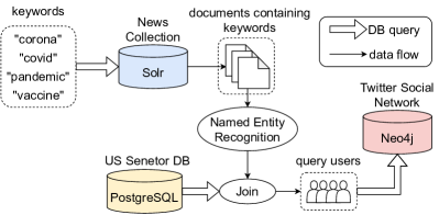
Figure 1. Illustration of PoliSci workload.

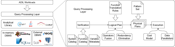
Figure 2. Illustration of the AWESOME system architecture.

Unfortunately, we find that most prior polystores do not support such rich analytics across these three data models. Furthermore, much prior art also aim to be highly general in supporting many stores, which often significantly restricts their ability to look into the specifics of the cross-engine dataflows to optimize their runtime performance at scale. In this work, we mitigate these issues by proposing a “tri-store” system focused specifically on relational, graph, and text analytics and elevating cross-engine dataflow optimization to the middleware. We call our system AWESOME: Analytics WorkbEnch for SOcial MEdia data. Table 1 summarizes the differences between AWESOME and key prior polystores (elaborated further in Section 8). We now explain the key desiderata and design decisions for our system.

1.1. System Desiderata and Design Decisions

• Tri-Model Dataflow Language. AWESOME must offer a unified high-level language to enable users to succinctly express tri-store analytics spanning relations, graph, and text. It should support “unistore-native” queries (e.g., SQL over RDBMS), basic control flows such as iteration and conditionals, and basic data types such as List and String to handle intermediates and pass arguments to unistore-native queries.

• Tri-Store Middleware. AWESOME must work transparently with underlying uni-stores to handle relational, graph, and text data. We use PostgreSQL, SQLite, Neo4j, Tinkerpop, and Solr as exemplars. Intermediate data must be handled automatically without manual exports/imports. In our PoliSci example, the named entities are joined with a PostgreSQL table and the join result must be passed to a Cypher query in Neo4j.

• Complex Analytical Functions. AWESOME must provide a set of popular complex analytical operators to support the tri-store analytics, including NLP algorithms on text and graph analytics algorithms. Extensibility via user-defined functions is desired. In our PoliSci example, the Solr query result is sent to an NER operator implemented by a popular NLP library.

• Execution Optimizations. AWESOME must support transparent physical query optimizations such as splitting computations across underlying unistores carefully and automatically caching (intermediate) data in memory when possible to reduce runtime. In our PoliSci example, NER returns a table that is much larger than the senators table in PostgreSQL. So, loading the senators table into memory to process the join in memory can be faster than pushing down the NER result to PostgreSQL.

• Strict Validation Mechanism. Some analytical operations such as PageRank are time-consuming and run-time errors/exceptions (e.g., type mismatch) lead to high overheads. So, a rigorous semantics check mechanism at compile time is needed to avoid runtime errors as much as possible.

1.2. Technical Contributions

In summary, this paper makes the following technical contributions.

• We present a formal description of ADIL, a dataflow language straddling relations, graphs, and text data models with rigorous semantics that enables the expression of complex workloads. An early version of ADIL was briefly introduced but not formalized in (Dasgupta et al., 2016).

• We present the architecture of AWESOME, the first optimized tri-store system to enable rich data science over social media data at scale, spanning relations, graphs, and text data. Figure 2 illustrates our system architecture. AWESOME automates handling of intermediate data to enable seamless user experience.

• We formalize the logical and physical levels of query planning in AWESOME. We present a suite of transparent optimizations to reduce runtime, including reducing data movement, placing computations in memory, careful apportioning of resources, and a cost model-based selection of execution plans.

• We present an extensive set of experiments using real-world datasets to demonstrate AWESOME’s support for rich social media analytics, while also enabling higher scalability and runtime efficiency than baseline approaches based only on an RDBMS or in-memory Python.

Table 1. Features of existing polystore systems and AWESOME.

	Language					System Design
	Native DBMS Query	Function	Graph Analytics	Text Analytics	Control Flow	Native Tri- Data Model	RDBMS Support	Graph DBMS Support	Text DBMS Support	In-memory DBMS Support
BigDAWG (She et al., 2016)	✓						✓		✓
Rheemix (Kruse et al., 2020; Agrawal et al., 2018)		✓	✓	✓	✓		✓
Estocada (Alotaibi et al., 2020)	✓						✓		✓
Tatooine (Bonaque et al., 2016)	✓						✓	✓	✓
Myria (Wang et al., 2017)	✓	✓	✓		✓		✓
Hybrid (Simmons et al., 2017; Podkorytov and Gubanov, 2019)	✓	✓					✓			✓
AWESOME	✓	✓	✓	✓	✓	✓	✓	✓	✓	✓

2. ADIL: A Dataflow Language

ADIL, the surface language for AWESOME, is designed as a dataflow language. The user expresses an analysis workload in ADIL as a sequence of assignment statements where the LHS of the assignment is a variable or multiple variables and the RHS is an expression. Figure 3 presents the ADIL script for the PoliSci workload.

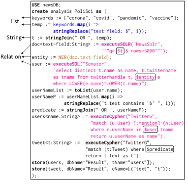
Figure 3. PoliSci represented in ADIL.

2.1. Data Types

ADIL supports the following data types in native. We annotate the data types for some variables in Figure 3.

• Primitive types: Integer, Double, String, and Boolean.

• Relation and Record: A Relation variable represents a relational table and a Record variable is a single tuple of a relation.

• Property Graph and Graph Element: Users can construct, query against, or apply analytical functions (e.g., PageRank) on property graphs. A GraphElement variable can be either a node or an edge with labels and properties.

• Corpus and Document: A Corpus is a collection of documents, and each document consists of document content (String), a document identifier (Integer) and tokens (List¡String¿).

• Matrix: We support Matrix data type and commonly-used matrix operators such as dot products on matrix-valued variables. In addition, an AWESOME matrix has optional row map and column map properties which are semantic mappings from matrix row (resp. column) indices to values in another data type. For example, for a document term matrix, the row map is a mapping from row indices to the document ids and the column map is a mapping from column indices to terms (i.e., tokens).

• Collection: A List is a collection of indexed elements with homogeneous type; a Tuple is a finite ordered sequence of elements with any type. List data type is strictly homogeneous: each element should have the same type. However, there can be heterogeneous objects in a Tuple variable. For example, the following tuple $T$ contains a relation, a graph, a list and constant values.

  R := executeSQL(..., ...); //produces relation RG := BuildGraphFromRelation(...); //produces graph GT := {R, G, [1, 2, 3], "string", 2 };

In this paper, Relation, PropertyGraph and Corpus types are collectively referred to as the “constituent data models” because they correspond to the data models of underlying stores.

2.2. ADIL Workload Structure

An ADIL script starts by declaring a polystore instance registered in AWESOME system catalog:

USE newsDB;create analysis NewsAnalysis as {/*main code block*/}AWESOME system catalog is a file that maintains the metadata for each user-defined polystore instance including the alias, connection detail, and schema of data stores in this instance. For underlying data store which admits a schema (e.g., PostgreSQL, Solr), a copy of the schema is maintained in the catalog. For stores that do not admit a schema (e.g., Neo4j), a set of schema-like information (e.g., node/edge labels/properties) is maintained. In the above example, the metadata of polystore instance newsDB will be retrieved from the system catalog which contains the information of all DBMSs used in the workload named NewsAnalysis.

The main code block contains a sequence of assignment statements (Section 2.3) and store statements (Section 2.4).

2.3. Assignment Statement

An ADIL assignment statement evaluates an RHS expression and assigns the result to one or more LHS variables. The grammar for assignment statement is shown as follows.

¡assignment-statement¿ ::= ¡var1¿ ‘, ’ ¡var2¿ ‘, ’ $\cdots$ ‘:=’ ¡assign¿

¡assign¿ ::= ¡basic-expr¿ — ¡ho-expr¿ The RHS expression (¡assign¿) can be “basic” or “higher-order” explained by the following grammar fragments, ¡basic-expr¿ ::= ¡const¿—¡query¿—¡func¿

¡ho-expr¿ ::= ¡assign¿ ‘¿’ — ‘==’ — ‘¡’ ¡assign¿ ¡var¿‘.map(’ ¡lVar¿ ‘-¿’ ¡assign¿ ‘)’ ¡var¿‘.reduce((’ ¡lVar1¿ ‘,’ ¡lVar2¿ ‘) -¿’ ¡assign¿ ‘)’ ¡var¿ ‘ where ’ ¡assign¿

2.3.1. Basic Expression

¡basic-expr¿ includes three types:

Constant Expression (¡const¿): A constant expression evaluates to a constant of any allowed data type. The expression can itself be a constant, e.g., [’x’, ’y’, ’z’], or a prior constant variable, or an element of a prior collection variable, e.g., a[1].

Query Expression (¡query¿): A query expression executes a query against a data store or against an AWESOME variable with a constituent data model. It uses standard query languages: SQL-93 for relational queries, OpenCypher (Francis et al., 2018) for property graph queries, and Lucene (McCandless et al., 2010) for retrieval from text indices. In Figure 3, three query expressions are marked in pink and they use executeSOLR, executeSQL and executeCypher keywords respectively. The first argument of a query expression is the alias of target DBMS registered in the polystore instance. If the query is against a variable created in prior statements, the first argument is left empty. The second argument is a standard Lucene/SQL/Cypher query with the exception of the $ followed by a variable name (highlighted by the rounded rectangles in the figure). ADIL uses $ as a prefix of the variable passed as a parameter to a query.

Function Expression (¡func¿): AWESOME supports a rich native library for common data analytical tasks. The expression includes function name with required positional parameters followed by optional and named parameters. A parameter can be a constant or a variable. The expression can return a single or multiple variables. The NER function expression marked as brown in Figure 3 takes a relation variable as parameter and returns a relation variable.

2.3.2. Higher-Order Expression.

A higher-order expression is recursively defined where another expression serves as its sub-expression. The following snippet from NewsAnalysis workload shows an example statement where the RHS is a nested higher-order expression:

wtmPerTopic := topicID.map(i =>        WTM where getValue(_:Row, i) > 0.00);topicID is a list of Integers and WTM is word-topic matrix where each row presents a word’s weights on all topics. For each topic, it produces a word-topic matrix consisting of words with weights higher than 0 on this topic. This snippet contains map, filter and binary comparison which are explained as follows.

Map Expression: A map expression operates on a collection variable, evaluates a sub-expression for each element in the collection, and returns a new collection object. The sub-expression can be a constant, a query, a function or another higher-order expression. In this snippet, it takes a list of integers (topicID) as input, and for each, applies another higher-order expression (a filter expression) on the WTM matrix to generate a matrix. Thus the returned variable (wtmPerTopic) is a list of matrices.

Filter Expression: The filter expression is indicated by the where clause – its sub-expression is a predicate; it returns a new collection with values which satisfy the given predicate. Since a matrix can be iterated by rows or by columns, users need to specify the iteration mode: the underscore sign ($\_$) is used to represent every single element in the matrix, and the colon ($:$) followed by the type specify the element type. In the example snippet, it applies a binary comparison predicate on each row of the matrix and returns a new matrix consists of the rows satisfying the predicate.

Binary Comparison and Logical Operations: A binary comparison accepts two expressions and compares their values to return a Boolean value. In the example above,

getValue(_:Row, i) > 0.00

checks whether the $i$-th element of a row vector is positive. More generally, ADIL supports any binary logical operators such as AND, OR and NOT over predicates.

Reduce Expression: A reduce operation aggregates results from a collection by passing a commutative and associative binary operator as its sub-expression. For example, the following snippet

R := relations.reduce((r1,r2) => join(r1,r2,on="id"))takes a list of relations as input and then joins each two tables and returns a new table at the end.

2.4. Store Statement

A store statement specifies the variables to be stored to a persistent storage, which can be an underlying DBMS registered in the system catalog or the AWESOME file system; it also includes the instructions for how to store the variable. In Figure 3, the last two lines store users and tweet variables to relational DBMS, and specifies the DBMS alias (dbName parameter), table name (tName optional parameter) and mapping between the targeted column names to the relational variables’ column names (cName optional parameter).

2.5. Some Properties of ADIL

A full discussion of the formal properties of ADIL is beyond the scope of this paper. Here we provide a few properties that will be useful in validating and developing logical plans from ADIL scripts.

1. ADIL does not have a for loop or a while operation. Instead, it uses the map operation to iterate over a collection and apply function over each element, the filter operation to select out elements from a collection that satisfies predicates, the reduce operation to compute an aggregate function on a collection. In ADIL, the collection must be completely constructed before the map (resp. filter or reduce) operation can be performed. Therefore, these operations are guaranteed to terminate.

2. ADIL is strongly typed.

3. In an assignment where the RHS expression is a query in a schemaless language like OpenCypher, the user must specify a schema for the LHS variable in the current system.

4. The data type and some metadata information of any LHS variable can be uniquely and correctly determined by analyzing the RHS expression (see Section 4).

3. System Architecture

The system architecture of AWESOME polystore is shown in Figure 2. We summarize some primary architectural components:

(a) Data Stores. It supports on-disk DBMSs (Neo4j, Postgres and Solr) and in-memory DBMSs (Tinkerpop and SQLite).

(b) Analytical Capability. It incorporates existing analytical libraries for NLP and graph algorithms such as CoreNLP and JGraphT, and AWESOME native functions written in Java.

(c) Query Processing. The “query” in AWESOME is essentially a multi-statement analysis plan consisting of data retrieval, transformation, storage, function execution and management of intermediate results. The query processor verifies an ADIL script, creates the optimal logical plan, generates a set of physical plans and then applies cost model and data parallelism mechanism to create an optimal execution plan.

4. Validating ADIL Scripts

An ADIL script is complex with many expensive operations. To reduce the avoidable run-time errors, AWESOME implements a strict compile-time semantics check mechanism which consists of two parts: 1) Validation refers to determining the semantic correctness of each expression, 2) Inference refers to inferring the data type and metadata of the variables generated from each expression.

4.1. Validation

For different RHS expressions, the validation process is different.

System catalog based validation. To validate a query expression (¡query¿) against an external DBMS, the system catalog is used to get the schema information. For example, for a SQL query, it checks if the relations and columns in the query exist in the database.

Function catalog based validation. For a function expression, AWESOME checks if the data types of the input variables/constant values are consistent with the parameters information registered in the function catalog.

Validation with Variable Metadata. Variable metadata map stores the key properties of variables and is built through inference process. It is looked up for every expression containing a variable. For a query expression, if it queries on relation-valued variables, their schema is found from the variable metadata map instead of the system catalog. For a function expression, if an input parameter is a variable, its data type will be found in the map.

Validation Example. Usually, more than one types of validation need to be used. We use the example snippet from Sec. 2.3.2 to show how to validate a nested higher-order expression. To validate the Map expression, it gets the data type and element type of topicID from the variable metadata map, then it checks if the variable has a collection type and the element type will be used to validate the sub-expression which is a Filter expression; to validate the Filter expression, similar to the Map expression, the data type of WTM is checked and the element type is used to validate the sub-expression which is a binary comparison expression, besides, it also checks if the return type of the sub-expression is a Boolean; to validate the binary comparison expression, it validates if the two operands have the same data type and the data type is comparable: in this example, the type of the left operand can be inferred based on the function catalog; At the end, it checks the getValue function using the element type information of WTM and topicID.

4.2. Inference

Inference refers to building variable metadata map. Table 2 in the technical report shows the variable types, and their corresponding metadata properties. For each statement in an analysis plan, the RHS expression is validated and then the type and metadata of the LHS variables are inferred as much as possible and be stored in the map.

Table 2. Metadata for different data types.

Data Type	Metadata
Relation	Schema $S=\{\textit{ColName}:\textit{Type}\}$
Property Graph	Node labels set $NL$ Node properties map $NP=\{\textit{PropName}:\textit{Type}\}$ Edge labels set $EL$ Edge properties map $EP=\{\textit{PropName}:\textit{Type}\}$
List	Element type, Element metadata, Size
Tuple	Each element’s type and metadata, Size
Map	Key type, Key metadata, Value type, Value metadata, Size
Matrix	Row (and column) count, Element type

The inference mechanisms are different for different expressions. For a SQL query expression, the schema of the returned relation is inferred by parsing the SELECT clause and looking up the system catalog/variable metadata map to get column types. For function expressions, the return types reside in the function catalog. For example, the following expression invokes function lda. By querying the function catalog, we know that it outputs two matrix variables. Thus the data types of DTM and WTM will be set as Matrix.

DTM, WTM := lda(processedNews,              docid=true, topic=numTopic);For nested expressions, the inference is handled from the innermost expression to the outermost expression. Taking the snippet shown in Sec. 2.3.2 as an example, the LHS variable’s type and metadata is inferred by the following steps: 1) the Filter expression returns a matrix since WTM is a matrix; and 2) Map expression will return a list of matrices since its sub-expression returns a matrix.

5. Logical Plan

After validating the correctness of an ADIL script, a logical plan will be constructed. A logical plan is a DAG where each node represents a logical operator.

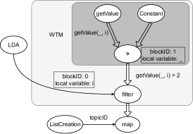
Figure 4. Logical plan of higher-order expressions.

5.1. Logical Plan Creation

The initial logical plan is directly translated from the parsing results. In most cases, each expression in the ADIL script corresponds to a single logical operator. For example, an ExecuteSQL query expression will be mapped to an ExecuteSQL logical operator. However, for specific functions expressions or higher-order expressions, extra processing steps are required to generate the initial logical plan.

Input-based Function Translation. For analytical functions, the corresponding logical operators can vary based on different function inputs. Table 3 presents some functions. For example, the function LDA can take either a Matrix variable or a Corpus variable as input, which corresponds to logical operators LDAOnTextMatrix and LDAOnCorpus respectively.

Higher-order Expressions to Sub-plans. For higher-order expressions (e.g., map expressions), a single expression will be translated to a sub-plan since it contains sub-expressions. For the nested higher order expression shown in Section 2.3.2, the logical plan is given in Figure 4. In Figure 4, there are two types of edges denoting data flow and sub-operator consumption, respectively. The Filter operator takes data from LDA and applies a binary comparison sub-operator. The Map operator takes data from ListCreation and applies the Filter sub-operator on each element of the data. Both Map and Filter create a local variable to denote each element of a collection, and the scope of such local variable is the sub-expression block of that higher-order expression.

Table 3. Some of ADIL functions and logical operators.

ADIL Function	Input Parameter	Logical Operator(s)
Preprocess	Column List<String> Corpus	CreateCorpusFromColumn CreateCorpusFromList NLPAnnotator(tokenize) NLPAnnotator(ssplit) NLPAnnotator(pos) NLPAnnotator(lemma) FilterStopWords
NER	Column List<String> Corpus AnnotatedCorpus	CreateCorpusFromColumn CreateCorpusFromList NLPAnnotator(tokenize) NLPAnnotator(ssplit) NLPAnnotator(pos) NLPAnnotator(lemma) NLPAnnotator(ner)
TopicModel	TextMatrix	TopicModelOnTextMatrix
	Corpus	TopicModelOnCorpus
LDA	Matrix	LDAOnTextMatrix
	Corpus	LDAOnCorpus
SVD	Matrix	CreateTextMatrix SVDOnTextMatrix
	Corpus
Sum	List	Column2List GetVector SumList SumVector
	Column
	Vector
	Matrix, Index

5.2. Logical rewriting

After creating the initial logical plan, a set of rewriting rules will be applied to generate an optimized logical plan.

Rule 1: Function decomposition. Some functions can be decomposed to several logical operators to achieve a deeper level of optimization. For example, for NER function which recognizes named entities in corpus, it will be translated to a series of CoreNLPAnnotator operators with different annotation sub-operators.

Rule 2: Redundancy elimination. The same operators which take the same input data will only be executed once. As Table 3 shows, some functions may share common logical operators, and these common operators will be merged.

Rule 3: Operators fusion. There are two special operators which apply a sub-operator on each single element of a collection variable: Map and NLPAnnotator. For a series of Map or NLPAnnotator, they will be fused and the sub-operators of them will be connected, which are termed as Map Fusion and NLP annotation pipeline. Figure 5 shows an example that corresponds to a snippet of workload NewsAnalysis, the left plot is the initial logical plan, and the right one applies map fusion. This rewriting has two advantages: 1) the intermediate results will not be materialized which saves memory. 2) it will benefit the candidate physical plans generation which will be discussed in detail in the physical planning section (Section 6).

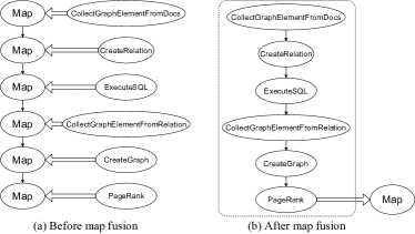
Figure 5. Illustration of map fusion.

Supposing the following ADIL snippet,

    processedDoc:= Preprocess(doc);    entity:= NER(doc);Figure 6 illustrates the aforementioned rewriting rules. The first part is the initial logical plan, and the second part shows the plan after applying the function decomposition rule. For the third part, functions Preprocess and NER share a series of common logical operators which are merged based on Rule 2. The final part applies Rule 3 to generate an NLP annotator pipeline, which is a common practice in NLP toolkits such as Standford coreNLP.

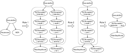
Figure 6. An Illustration of logical plan rewriting rules.

6. Physical Plan

Based on the optimized logical plan, we introduce the physical planning details of AWESOME. As shown in Algorithm 1, there are mainly three steps to generate the candidate physical plans, each of which will be introduced in the following sections.

Input: A logical plan $G=(V,E)$, a boolean flag $buffer$.

Output: Candidate physical plans: $candPlans$

1 $candPlans\leftarrow$ CandidatePhsicalPlanGen ($G$);

2 $candPlans\leftarrow$ AddDataParallelism ($candPlans$);

3 if $buffer$ then $candPlans\leftarrow$ AddBuffering ($candPlans$);

Algorithm 1 Physical Plan Generation

6.1. Candidate Physical Plans Generation

We introduce the pattern based transform algorithm to generate a set of candidate physical plans from a logical plan DAG. To begin with, we provide some definitions as follows.

Definition 6.1 (Pattern Set).

A pattern set $Pat:\{\{OP^{l},E^{l}\}\to\{\{OP^{p},E\}\}\}$ is a mapping where a key is a logical sub-DAG and a value is a set of physical sub-plans. The pattern set is ordered by the sizes of keys (i.e., the numbers of nodes in the logical sub-DAGs) to make sure that in the subsequent procedures the larger patterns in a logical plan are matched earlier.

Definition 6.2 (Candidate Physical Plans).

Candidate physical plans consist of a DAG $PG=\{OP^{p},E\}$ which contains some virtual nodes, and a map $PM:I\to\{OP^{p},E\}$ where a key is a virtual node id and a value is a set of physical sub-plans.

Input: An ordered pattern set $Pat$; An optimal logical plan DAG $G=(V,E)$.

Output: Candidate physical plans: $PG$ and $PM$.

1 $PG\leftarrow G,PM\leftarrow\{\}$;

/* match patterns from the largest to the smallest. */

2 for $pat\in Pat$ do

3       $pSubs\leftarrow Pat[pat]$;

4       $lSubs\leftarrow$ FindMatchPattern ($PG,pat$) ;

5       for $sub\in lSubs$ do

             /* for a pattern which only has one physical sub-plan, directly replace the pattern with the DAG. */

6             if $pSubs.size==1$ then

7                   $PG\leftarrow$SingleOperatorTransform ($PG,sub,pSubs$);

8                  

            /* for a pattern with several candidate physical sub-plans, transform $sub$ to a virtual node and add the node id and physical sub-plans to map $PM$. */

9             else

10                   $PG,PM\leftarrow$ PatternTransform ($PG,PM,sub,pSubs$);

11                  

Algorithm 2 Candidate Physical Plan Generation

We propose Algorithm 2 to generate the candidate physical plans. Table 4 lists some logical operators and their corresponding physical operators. For some logical operators like LDAOnCorpus or some logical sub-DAGs, each corresponds to only one candidate physical operator or sub-plan. In this case, each operator or sub-DAG will be directly replaced by the physical operator or sub-plan (lines 6-7). On the other hand, there exist logical operators or sub-DAGs corresponding to multiple candidate physical operators or sub-plans. For example, in Figure 7, a logical sub-DAG CreateGraph $\to$ ExecuteCypher can be transformed to multiple different physical sub-plans shown in the dashed rectangle marked by Node 1. In this case, the operator or sub-DAG will be replaced by a virtual node, and the virtual node ID with its corresponding physical sub-plans will be stored in the map $PM$ (lines 8-9).

Table 4. Summary of AWESOME logical and physical operators.

Types	Logical Operators	Physical Operators	DataParallelCap	BufferingCap
Query	ExecuteCypher ExecuteSQL ExecuteSolr	ExecuteCypherInNeo4j ExecuteCypherInTinkerpop ExecuteSQLInPostgres ExecuteSQLInSQLite ExecuteSolr	ST EX ST EX ST	SO SO SO SO SO
Graph Operations	BuildWordNeighborGraph BuildGraphFromRelation PageRank	CollectGraphElementsFromDocs CollectGraphElementsFromRelation CreateTinkerpopGraph CreateNeo4jGraph PageRankTinkerpop	PR PR ST ST EX	SS SS SI SI SO
Text Operations	NLPAnnotator LDAOnCorpus TopicModel	CreatDocumentsFromRecords CreatDocumentsFromList CreateTextMatrix LDAOnCorpus SVD	PR PR PR EX EX	SS SS SS SI B

Figure 7 shows the candidate physical plans for the logical plan in Figure 5. There are two virtual nodes and each corresponds to several physical sub-plans. This figure also shows the advantage of Map Fusion which connects all the sub-operators of a series of Maps so that the sub-DAG matched with a pattern in the pattern set could have larger size and thus leads to more efficient candidate plans. For example, after map fusion, the CreateGraph$\to$ExecuteCypher pattern will be translated to three physical sub-plans. However, without map fusion, the CreateGraph itself will be translated to three candidate operators: CreateTinkerpopGraph, CreateNeo4jGraph and CreateJgrapht, since the JgraphT library does not support Cypher queries, if CreateJgrapht is chosen during execution, then it will initiate a set of typecasting transformations before executing ExecuteCypher, which increases the overall cost.

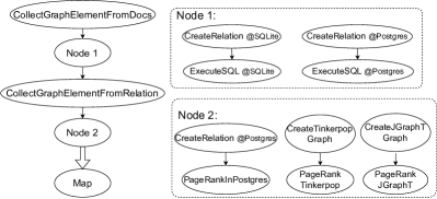
Figure 7. Candidate physical plans for Figure 5 logical plan.

6.2. Partitioned Data Parallelism

AWESOME exploits data parallelism to take advantage of modern multi-core systems. Table 4 presents some physical operators with their data parallel capabilities. ST means single-threaded operators which can not be executed in a data parallel fashion, PR means data parallelizable operators, and EX means operators provided by external libraries. The execution of EX operators is fully supported by external libraries and can utilize multi-core feature in their native implementation, and thus they are excluded from the subsequent AWESOME optimizations which are based on data parallelism.

For a PR operator with multiple inputs, it is associated with a $capOn$ attribute specifying the input on which it has data parallelism capability. For example, the FilterStopWords operator takes a corpus and also a list of stop-words as input, and it can be executed in parallel by partitioning the corpus input. In this case, $capOn$ will be set as the ID of the corpus variable. Every PR operator will be executed in parallel by partitioning the $capOn$ input data. Figure 8 shows an illustration. The left sub-figure shows the original physical plan DAG and the right sub-figure shows the plan DAG after considering data-parallelism. When an operator with PR capability gets its input: if its $capOn$ input was not partitioned, a Partition step will be added which generates partitioned result; if a non-$capOn$ input was partitioned, then a Merge step will be added to collect data from multi-threads to a single collection; When an operator with ST capability gets data from an operator with PR capability, a Merge step will be added.

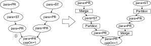
Figure 8. Illustration of data parallel execution.

6.3. Buffering Mechanism

AWESOME employs a buffering mechanism to avoid storing unnecessary intermediate results in memory. Different from pipeline, buffering mechanism does not utilize multiple cores to execute different operators simultaneously. Some operators can process input in a batch-by-batch manner, and some can generate output in a batch-by-batch manner. We refer data with this manner as stream hereafter. There are four types of buffering capabilities:

1. $SI$ (Stream-Input): the input can be passed as stream to the operator, but it produces a whole inseparable result at once;

2. $SO$ (Stream-Output): the operator takes an inseparable input but can produce result progressively as stream;

3. $B$ (Blocking): both the input and output need to be a whole;

4. $SS$ (Stream-Stream): both the input and output can be a stream.

Each physical operator is associated with its buffering capability. Table 4 presents it for some physical operators. Similar to data parallelism capability, there is another $capOn$ attribute associated if the operator has more than one input. The physical DAG will be partitioned to a collection of chains. Inside each chain, the intermediate result is not stored in memory; the upstream operator produces stream output to be consumed by the downstream operator. The data across chains has to be stored in memory.

The collection of chains is collected from the physical DAG by partitioning it based on the partition rules which are shown below and also illustrated in Fig. 9:

• For an edge $e=(op_{e1},op_{e2})$, if $op_{e1}$ can’t generate stream result or $op_{e2}$ can’t take stream input, $e$ will be cut. For example, in Fig. 9, the edge between $op_{1}$ and $op_{21}$ is cut.

• For an edge $e=(op_{e1},op_{e2})$, if data from $op_{e1}$ to $op_{e2}$ is not the $capOn$ input of $op_{e2}$, $e$ will be cut. In Fig. 9, the edge between $op_{22}$ and $op_{12}$ is cut.

• For an operator $op$, if it has more than one outgoing edges, then all outgoing edges will be cut. In Fig. 9, the outgoing edges from $op_{2}$ are all cut.

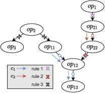
Figure 9. Illustration of buffering rules.

AWESOME users have the option to turn on buffering mechanism. The buffering mechanism would be very helpful if : 1) the analysis plan contains many data flow edges which buffer can be added to; or 2) AWESOME is running on a memory-limited machine; or 3) users care about the responsiveness of the system and expect to get some initial results back soon without waiting for the complete results.

6.4. Failed Attempt: Pipeline + Data Parallelism

We built a framework that hybridizes pipeline (i.e., task parallelism) and data parallelism, however, the experimental results reveal that such framework is not suitable for AWESOME. We briefly introduce this framework and explain why this technique did not boost performance to provide some insights for future researches.

Similar to the buffering mechanism, an AWESOME physical DAG is partitioned into a list of chains based on the partition rules. Then each chain will form a pipeline where operators can be executed simultaneously using multi-cores. Once the upstream operator produces a batch of results, the downstream operator will be executed on that batch immediately and simultaneously. Both pipeline and data parallelism utilizes multi-cores to increase resources utilization, thus we define a scheduling problem to allocate a specific amount of cores (the number of cores in an OS) to operators in each pipeline chain. A simple solution is to allocate cores to match the produce and consume rates of data.

However, from the experimental results, this framework is not more efficient than data parallelism framework even under the best allocation strategy due to two properties of AWESOME operators. We theoretically explain the reason why this framework does not outperfrom data parallelism framework. For a simple pipeline chain with two operators: $op_{1}\to op_{2}$, suppose that there are a total of $n$ cores and it costs $t_{1}$ for $op_{1}$ to produce a batch of data and $t_{2}$ for $op_{2}$ to consume the batch, then there will be $t_{1}n/(t_{2}+t_{1})$ cores assigned to $op_{1}$ and the rest of cores assigned to $op_{2}$.

Suppose that $op_{1}$ will produce $m$ batches in total, then the execution time of applying data parallelism solely $T_{1}$ and of applying pipeline + data parallelism $T_{2}$ can be computed as,

(1) $$\begin{split}T_{1}&=\frac{(t_{1}+t_{2})m}{n}+agg*n\\ T_{2}&=\max\{\frac{t_{1}m}{n_{1}},\frac{t_{2}m}{n-n_{1}}\}+agg*n_{1},\end{split}$$

where $n_{1}$ is the number of cores assigned to $op_{1}$, and $agg*\#core$ is the sequential aggregation cost of data parallelism. Since for AWESOME aggregation operators such as SUM, the aggregation cost is usually very small and can be negligible comparing to other time-consuming analytical functions, we can prove that $T_{1}\approx\frac{(t_{1}+t_{2})m}{n}\leq\max\{\frac{t_{1}m}{n_{1}},\frac{t_{2}m}{n-n_{1}}\}\approx T_{2}$ always holds where the equality is achieved when the above optimal allocation solution is applied. Thus, the pipeline and data parallelism framework can’t outperform data parallelism if all operators in a chain are data parallel-able.

Appendix D presents the data parallel capability and buffering capabilities for most AWESOME operators. In the future, when there are more operators with different properties are added to AWESOME, this framework may have chance to outperform the solely data parallelism framework.

7. Learned Cost model

The query planning stage generates multiple candidate physical plans, and in the execution stage, the optimal one will be chosen at run-time based on a learned cost model.

For each virtual node which corresponds to multiple candidate sub-plans, the cost model is applied to each sub-plan to estimate the execution cost and the sub-plan with the lowest cost will be chosen. We use a learned cost model instead of a rule-based model based on two reasons:

• Cost should be decided at sub-plan level instead of operator-level, which makes rule-based optimization hard to design. For a single logical operator with different physical implementations, it is easy to design rules to decide which implementation should be chosen under what circumstance. However, in the pattern set, each logical sub-plan may consist of several logical operators and each of them may be transferred to multiple different physical operators, leading to a large size of rules space.

• The cost of a physical operator may depend on several features and a rule-based model is too simple to represent the complex relationship.

7.1. Cost Model

We provide a learned cost model to estimate the execution time for each candidate physical sub-plan denoted as $S$. Suppose that $S$ consists of multiple operators $\{op_{1},\cdots,op_{n}\}$, the overall cost estimation is given as the sum of the estimated cost of all operators since AWESOME does not apply task parallelism, i.e.,

(2) $$est_{S}=Cost(op_{1})+\cdots+Cost(op_{n}),$$

where $Cost(\cdot)$ is a trained linear regression model with the polynomial of raw features (degree 2) as variables that predicts the execution cost of a physical operator, i.e.,

(3) $$\begin{split}Cost(op)=w_{0}+w_{1}f_{1}+\cdots+w_{n}f_{n}+w^{\prime}_{1}f^{2}_{1}+\cdots+w^{\prime}_{n}f^{2}_{n}\\ +w_{(1,2)}f_{1}f_{2}+\cdots+w_{(n-1,n)}f_{n-1}f_{n},\end{split}$$

where $f_{1},\cdots,f_{n}$ are the raw features for $op$. $Cost(op)$ is trained based on training data collected from calibration for operator $op$. For relation-related operators, the raw features include the sizes of tables; for graph-related operators, node count or edge count is selected as a raw feature and for some graph queries, the predicate size can also be a raw feature.

7.2. Calibration

To train the individual cost model $Cost(\cdot)$, we design a set of synthetic datasets which vary at some parameters, and run each operator on different datasets to collect a set of execution time.

Operators and features. We mainly train cost model for operators which are graph-related or relation-related.

For graph operators, we evaluate common operators such as CreateGraph and PageRank. The graph size serves as one feature for the cost estimation. For ExecuteCypher, there are various types of Cypher queries and we evaluate two typical types of queries: Type I: Queries with a series of node or edge property predicates. For example, Match (n)-[]-(m) where n.value in L and m.value in L where $L$ is a list of strings. The size of $L$ is another raw feature that decides the query cost.

Type II: Full text search queries. In this kind of queries, there is a node/edge property which contains long text and the queries will find out nodes/edges whose text property contains specific strings. For example, Match (n)-[]-(m) where n.value contains string1 or n.value contains string2 or …... The number of the OR predicates is another raw feature of the cost model.

For relation operators, we test the ExecuteSQL operator. Based on the locations of the tables in the query, there are different candidate execution sub-plans for this operator. For example, if all tables involved are AWESOME tables generated from the upstream operators, then there are two candidate plans: (a) store all relations to in-memory SQLite, and execute the query in SQLite; (b) store all relations in PostgreSQL, and execute the query in PostgreSQL. If there are both AWESOME tables and PostgreSQL tables involved in the query, the two candidate plans are illustrated in Figure 10(a): (a) as the left dashed rectangle shows, we store AWESOME tables to PostgreSQL, then execute the query in PostgreSQL; (b) as the right dashed rectangle shows, we store AWESOME tables to SQLite and select the columns needed from PostgreSQL tables and store them to SQLite, then the query will be executed in SQLite.

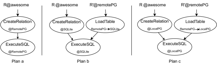
(a) Execution Sub-plans

(b) Row count of R: 100.

(c) Row count of R: 10K.

Figure 10. Execution sub-plans and calibration results for cross-engine ExecuteSQL. The part with ’//’ denote execution time of ExecuteSQL operator.

Datasets. We design a set of graph datasets and relation datasets which are used for graph- and relation-related operators respectively. We present the statistics in Table 5.

Table 5. Parameters of synthetic datasets for cost model.

	Parameter	Value
graph dataset 1	edge size	500, 1k, $\cdots$, 800k
	avg. density	2
	node property	value: String
	keyword size	50, 100, 500, 1k, 2k
graph dataset 2	node size	5k, 10k, $\cdots$, 500k
	node property	tweet: String
	keyword size	50, 100, 500, 1000
relation dataset	PostgreSQL table row count	100, 1k, 10k, 100k
	Awesome table row count	100, 1k, 10k, 100k

For graph datasets, there are two types of graphs: The first type of datasets is used to test operators including CreateGraph, PageRank and the Type I Cypher queries: We created several property graphs with different edge sizes, and to simplify the model we kept the density of graphs as a constant value 2; each node (or edge) has a value property which is a unigram and we make sure each node’s (or edge’s) property is unique, then we created keywords lists with different sizes from the values set as the predicates. The second dataset is designed for the Type II Cypher queries: We created graphs with different node sizes and each node has a tweet property whose value is a tweet text collected from Twitter; All the unigrams are collected from these tweets and after removing the most and the least frequent words, we randomly selected words to create different sizes of keywords lists which will be used to do text search.

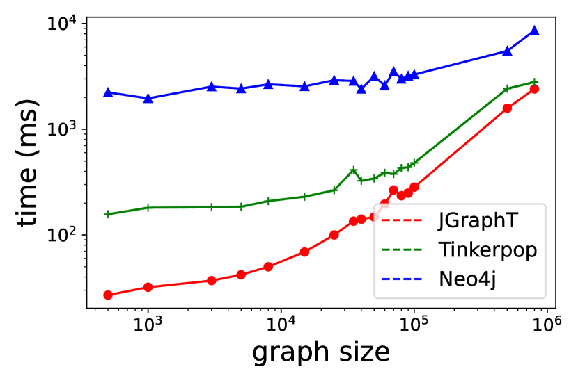
(a) Graph Creation

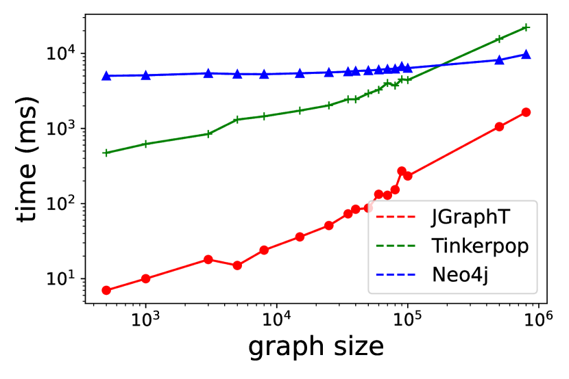
(b) Page Rank

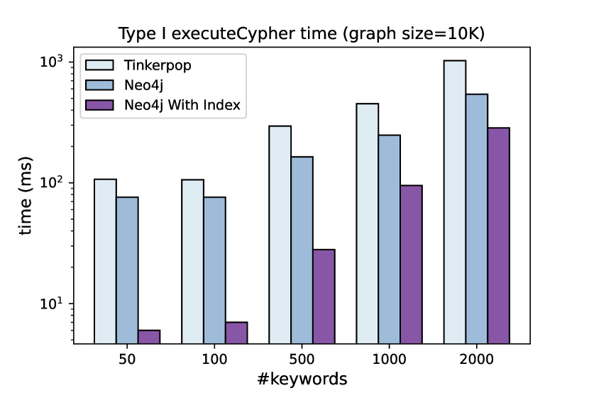
(c) Type I Cypher Query

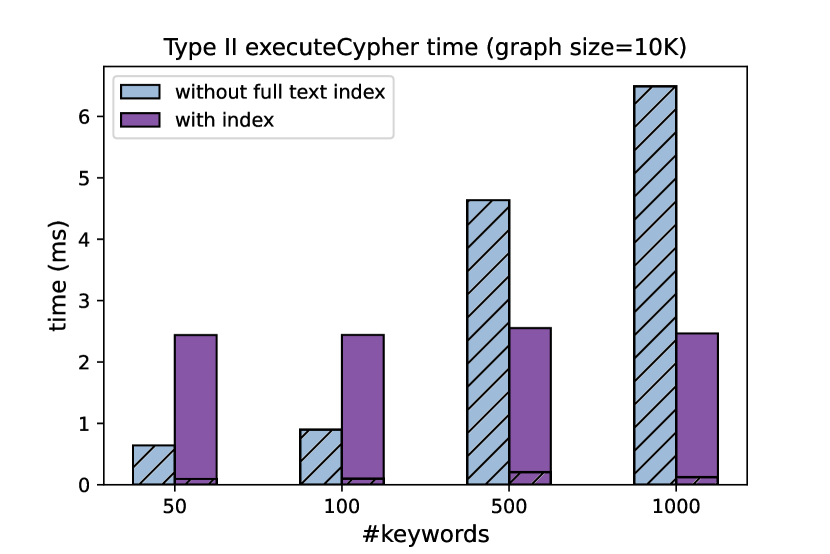
(d) Type II Cypher Query

Figure 11. Calibration results for graph operators

Calibration Results. We present some calibration results for some operators/patterns in Figure 11, Figure 10(b) and Figure 10(c). Figure 11 shows part of the calibration results for some graph operators. Figure 10(b) and 10(c) show the calibration results for the ExecuteSQL operator where the query includes a PostgreSQL table and an AWESOME table and the two sub-plans correspond to the sub-plans in Figure 10(a).

7.3. Training and Cost Estimation

The individual cost model for each operator is trained based on the calibration results to minimize the loss function, i.e., mean squared error. At run-time, when the input of a virtual node is returned from the upstream operator, the features are collected and passed to the overall cost model (Equation 2) to compute the cost for each candidate physical sub-plan. The best sub-plan with the lowest cost will be selected.

8. Experiments

In this section, we first empirically validate whether AWESOME is able to improve efficiency of analytical polystore workloads. Then, we drill into how the cost model of AWESOME contributes.

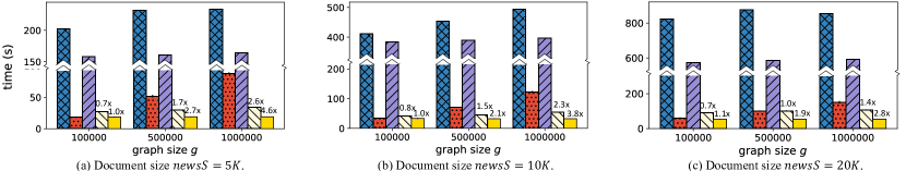
Figure 12. Total execution time for PoliSci w.r.t. different $newsS$.

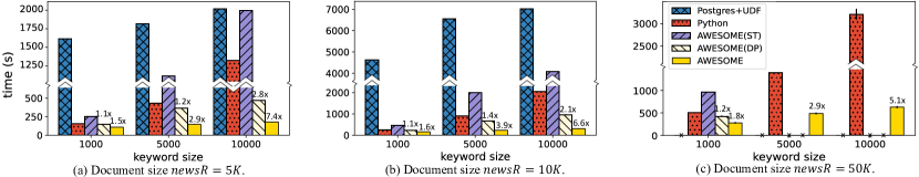
Figure 13. Total execution time for NewsAnalysis w.r.t. different $newsR$.

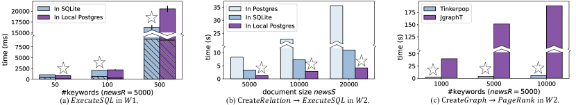
Figure 14. Execution time of different physical plans.

8.1. Experimental Setup

We focus on the single-machine multi-cores setting, and the distributed version of AWESOME will be our future work. The experiments were run on CloudLab (Duplyakin et al., 2019), a free and flexible cloud platform for research. The machine has 24-core AMD 7402P CPUs, 128 GB memory and 1.6 TB disk space. It runs Ubuntu 18.04.

Datasets. We collect four real world datasets to run the workloads.

• Newspaper: A relation stored in a PostgreSQL database aliased as News with size around 36 GB. There are over 1M news articles with an average length of 500 words collected from the Chicago Tribune newspaper.

• SenatorHandler: A PostgreSQL relation of about 90 United States senators with their names and twitter user names stored in PostgresSQL database aliased as Senator.

• NewsSolr: A collection of news stored in the Solr engine with size around 20 GB.

• TwitterG: Attribute graphs stored in Neo4j that represent the Twitter social networks of different sizes. A node in TwitterG is labeled as either “User” or “Tweet”. A User node has a property userName, and a Tweet node has a property tweet storing tweet content. A User node connects to another User node by a directed edge if the first one mentions the second, and a User node connects to a Tweet node by a directed edge if the user authors the tweet.

Workloads. We evaluate two analytical workloads. W1: PoliSci focuses on the polystore aspect of the system where input data is stored in heterogeneous data stores. W2: NewsAnalysis, a complex text analytical task, focuses on analytical functions including graph algorithm like PageRank (Page et al., 1999) and NLP functions like LDA (Pritchard et al., 2000).

The illustration and ADIL script of PoliSci are shown in Figure 1 and Figure 3. This workload queries on the NewsSolr, SenatorHandler and TwitterG dataset. For workload NewsAnalysis, the corresponding ADIL script is given in Appendix B. It selects news from News dataset and applies LDA model to detect topics from the corpus. Then it implements the method in (Gollapalli and Li, 2018) to evaluate the quality of each topic. Specifically, for each topic, from news corpus a word-neighbor graph is constructed which consists of the keywords in the topic and the aggregated PageRank value of these keywords in this graph will be used as a metric to evaluate the quality of the topic.

Parameter Settings. For the PoliSci workload, we change two parameters: 1) $newsS$, the size of documents $doc$ selected from NewsSolr dataset and is set by changing $rows=5000$ in the Solr query to different values. $newsS\in\{5K,10K,20K\}$. 2) the size of the graph $TwitterG$: the graph size, denoted by $g$, is the number of nodes in it. $g\in\{100K,500K,1M\}$. $newsS$ will have impact on the size of $entity$ and thus will influence the executeSQL execution time, and $g$ will influence on executing the two Cypher queries. For the NewsAnalysis workload, we vary two parameters: $newsR$ is the size of news selected from Newspaper relation: $newsR\in\{5K,10K,50K\}$; $t$ is the number of keywords in each topic: $t\in\{1K,5K,10K\}$ for the end-to-end experiments and $t\in\{50,100,500\}$ for the drill down analysis. $newsR$ and $t$ control the size of the documents and the size of the word-neighbor graph for each topic.

Compared Methods. We implement and compare the following methods. We put the SQL scripts for Postgres+UDF method and Python code for Python in Appendix A and C. For Postgres+UDF implementation, the scripts have around 400 and 1000 tokens respectively for the two workloads and Python codes have around 380 and 600 tokens for each. While ADIL scripts only have around 100 tokens for each.

• Postgres+UDF: It stores all datasets to a single store, Postgres, and uses pure SQL scripts with user-defined functions written in Python or implemented by MADLIB (Hellerstein et al., 2012) toolkit.

• Python: The workloads were implemented in Python. To make sure the results are the same as AWESOME’s and to make the comparison fair, for analytical functions such as LDA and NER, we use the same toolkits as used by AWESOME.

• AWESOME(ST): ST stands for single threaded. It does not use any AWESOME features including logical plan optimization, data parallel execution and cost model.

• AWESOME(DP): DP stands for data parallelism. It only applies data parallelism feature.

• AWESOME: It has full AWESOME features including logical optimization, cost model and data parallelism.

8.2. End-To-End Efficiency

For AWESOME baselines, the end-to-end execution time is the total execution time from taking a workload as input, parsing, validating, logical planning, physical planning and executing. For Postgres+UDF baseline, to make the comparison fair, we exclude the data movement cost, which is the time spent to move data from others stores to Postgres, from the total cost. Figure 14 and Figure 14 present the end-to-end execution costs of the four compared methods. The numbers on top of bars denote the speed-up ratio to the Python baseline. The black Xs mean that the program either pops out an error or can not finish in 3 hours.

From the results, AWESOME(DP) and AWESOME show great efficiency and scalability when varying the parameters. It dramatically speeds up the execution time over Postgres+UDF. For NewsAnalysis, when $newsR=50K$, Postgres+UDF pops out a sever connection lost error message when running in-Postgres LDA function. Comparing with AWESOME(ST), data parallelism achieves significant performance under any parameter setting. In the following, we mainly discuss the performance gain of AWESOME(DP) and AWESOME over the baseline method Python.

For workload PoliSci, when the graph size $g$ increases, AWESOME achieves an increasingly large speedup over the Python implementation. When $g=100K$, AWESOME(DP) is a little bit slower than Python, but with the cost model, AWESOME has similar performance as Python; When $g$ is increased to $1M$ and $newsS=5K$, AWESOME(DP) and AWESOME speeds up the execution time by $\sim 3$x and $\sim 5$x respectively.

For workload NewsAnalysis, when $newsR=5K$ and keywords size is large ($t=10K$), AWESOME(DP) and AWESOME can achieve up to $\sim 3$x and $\sim 7$x speed-up respectively over Python; when $newsR=50K$ and keyword size is $10K$, AWESOME(DP) pops out an out of memory error because it selected a bad execution plan, while AWESOME is scalable and can finish in around 10 minutes which is about $5$x speedup over Python.

Why not single DBMS with UDF? From our experience with implementing the Postgres+UDF, we found that this single DBMS with UDF setting fails to qualify polystore analytical tasks for three reasons: 1) Data movement cost. Users need to write ad-hoc code to move data from various stores to a single store. 2) Programming difficulty. It is not flexible to program with pure SQL. For workload NewsAnalysis, even with MADLIB toolkit which implements LDA and PageRank UDFs, hundreds of lines of SQL needed to be written (as shown in the Appendix A). 3) Efficiency. The in-DBMS implementation of analytical functions such as LDA and PageRank are much less efficient than using the mature packages from Java or Python, and the current in-DBMS implementation of some analytical functions is not scalable as well.

8.3. Drill-Down Analysis

We present some detailed evaluation results to explain how AWESOME achieves a better performance over AWESOME(DP).

We take some snippets from each workload and show the execution time of different candidate sub-plans for these snippets in Figure 14. The parts with “//” hatch denote execution time for ExecuteSQL physical operator. The bars with stars on top are the best execution plans selected by AWESOME cost model.

For workload PoliSci, Figure 14 (a) presents the execution time for different sub-plans regarding to the cross engine ExecuteSQL logical operator where one table ($SenatorHandler$ table) is from PostgreSQL and another (named entity table) is an AWESOME table. The three execution plans are illustrated in Figure  10(a). When the selected documents size increases, the named entity table’s size will increase and the in local Postgres execution plan will be much more effective than the in remote Postgres one by not moving large size of data to a remote Postgres server. In SQLite execution is not efficient because even though storing table data to in memory SQLite is fast, SQLite is slow when the two tables join on Text columns.

For workload NewsAnalysis, Figure 14 (b) shows the execution time for logical plan ExecuteSQL. The possible physical sub-plans are shown in Node 1 in Figure 7. The cost model does not look at each single operator, e.g., ExecuteSQL, to decide the best physical operator, instead, it looks at the sub-plan which consists of both creation and query execution to determine the best physical sub-plan. We selected some small keywords sizes for this drill down analysis: $t=\{50,100,500\}$ since when $t$ gets larger, the In-SQLite execution always dominates. As (b) shows, the SQL query execution time of local Postgres is less than that of SQLite, however, when considering both table creation time and execution time, the in-memory SQLite plan will be chosen for $t=\{100,500\}$. These results on small snippets demonstrate the effectiveness of our cost model.

We pick a snippet from NewsAnalysis to analyze the effectiveness of buffering mechanism:

rawNews := executeSQL("News", "select id as newsid,            news as newsText from usnewspaper            where src = $src limit 1000");processedNews := tokenize(rawNews.newsText,            docid=rawNews.newsid,            stopwords="stopwords.txt");This snippet is translated to a chain of physical operators where a buffer mechanism can be added to any two successive operators: ExecuteSQL $\to$ CreateCorpusFromColumn $\to$ SplitByPatterns $\to$ FilterStopWords. The number of documents retrieved by the SQL query is set as 1 million by changing the “limit” clause. The memory footprint is presented in Figure 15. Adding buffering mechanism decreases the used heap size from around 27 GB to about 17 GB ($\sim 37\%$ reduction) with a small run-time overhead ($\sim 8\%$ increase).

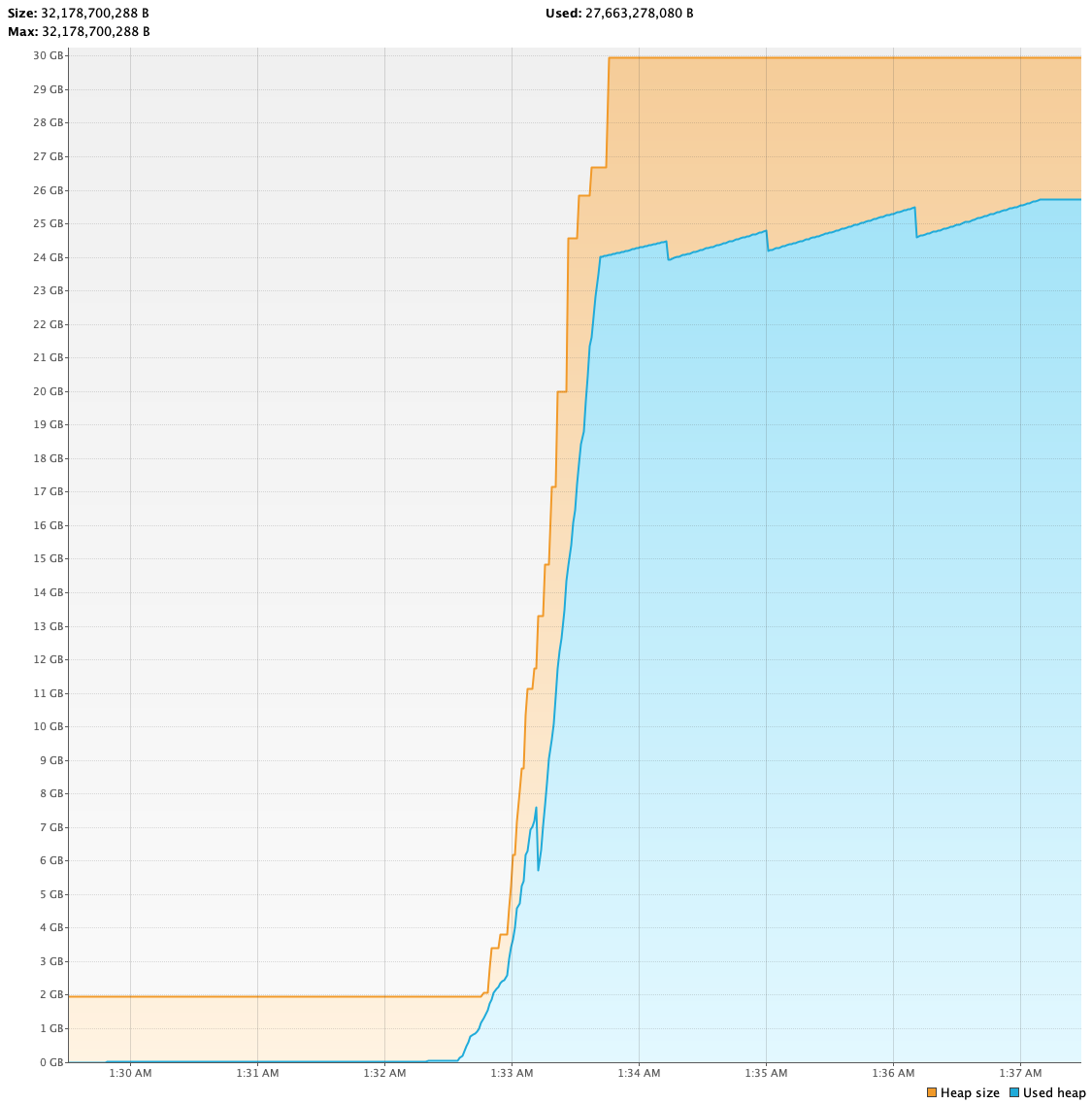
(a) Without buffering mechanism.

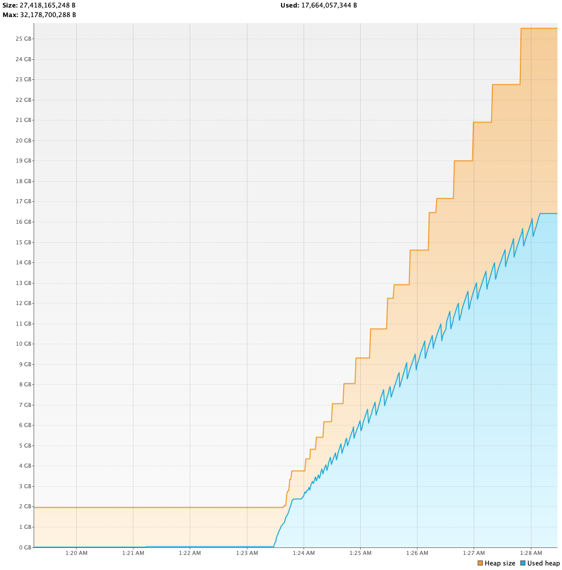
(b) With buffering mechanism.

Figure 15. Memory footprint of executing a chain.

9. Related Work

We present the features comparison of selected prior polystore systems and AWESOME in Table 1. Besides the systems shown here, there are some existing work (Lucas et al., 2018; Kruse et al., 2020; Khayyat et al., 2015; Gog et al., 2015; Doka et al., 2016) which focus on integrating multiple data processing platforms such as Spark, Hadoop, GraphX to process heterogeneous data. However, they do not focus on DBMSs, and hence are not discussed in detail in this paper. We conclude some important language and system design features for analytical polystores based on our experience working with domain scientists. As the table suggests, none of the prior polystore systems has all of these features.

9.1. Polystore Languages

BigDAWG (Duggan et al., 2015a; She et al., 2016; Duggan et al., 2015b), Estocada (Alotaibi et al., 2019, 2020) and Tatooine (Bonaque et al., 2016) all support querying backend DBMSs using native languages. However, they do not support analytical functions or any control flow logic such as IF-ELSE or For loop.

RheemLatin (Kruse et al., 2020; Lucas et al., 2018; Agrawal et al., 2018) is an extension from PigLatin (Olston et al., 2008). Similar to ADIL, it has its native data models and grammars; it has Loop operators to support tasks with iterations. Users write platform agnostic analysis plan using Rheem keywords which makes it easier to do query optimization but also brings several deficiencies: 1) For queries against DBMSs, it shows that users can express a SQL query in RheemLatin, however, it will be hard or impossible to rewrite a Cypher query or Solr query using Rheem keywords. 2) It does not support analytical functions such LDA or NLP annotations in native. Users can write an analytical function as a combination of RheemLatin keywords, however, it requires a lot of programming efforts and expert knowledge.

Myria (Wang et al., 2017) provides a hybrid imperative-declarative query language called MyriaL. It consists of a sequence of assignment statements where the left-hand sides are relation variables and the right-hand sides can be a SQL query, comprehensions, or function calls. It also supports flow control logic such as DO-WHILE structure. However, SQL is the only supported query language.

Hybrid.Poly (Podkorytov et al., 2017; Podkorytov and Gubanov, 2019) provides a hybrid relational analytical query language stemming from SQL which is based on their extended relational model. It uses an SQL-like language where analytical functions (e.g., dot products) are specified in the SELECT clause, but it does not provide built-in text or graph analytical functions.

9.2. Polystore Systems

All of these polystore systems support RDBMS, but to the best of our knowledge, none of them support both graph and text DBMS. Among all of them, only Hybrid supports in-memory database engines. We conclude some design details for selected systems.

BigDAWG (Duggan et al., 2015a; She et al., 2016; Duggan et al., 2015b) organizes storage engines into a number of islands. An island is composed of a data model, a set of operations and a set of candidate storage engines. It supports heterogeneous data models including relational tables and arrays, and supports cast functions to migrate data from one island with one data model to another island with a different model. To our best knowledge, BigDAWG does not support graph DBMS or analytical functions.

The Rheemix system (Kruse et al., 2020) is a cross-platform system built over diverse engines including PostgreSQL, Spark, Flink and Java Streams. In Rheemix, analytical tasks are specified as a workflow of Rheemix operators (e.g., filter, map, groupBy) that are directly mapped to operators of the underlying systems through operator inflation. Their operators are primitive (fine-granular) operators, which makes optimization easier at the cost of expressiveness.

Hybrid.Poly (Podkorytov et al., 2017; Podkorytov and Gubanov, 2019), a relationally backed in-memory polystore system, only uses one consolidated parallel engine as a back-end to store all data. It decomposes a full analysis into a series of analytical queries where variables are passed by explicitly creating tables of intermediate results. It extends the relational data model with additional types and operations to support matrix and vector abstractions and operators over them. Different from AWESOME, it does not support text or graph data models or any on-disk databases.

Our general observation is that, while there is a clear growth in creating and using polystores for different applications, no existing polystore system supports all requisite features needed by domain scientists to solve a variety of real-world analytical workloads.

10. Conclusion and Future Work

In this work, we empower an emerging class of large-scale data science workloads over social media data that naturally straddle analytics over relations, graphs, and text. In contrast to complementary work on polystores that aim for high generality, we build a more specific tri-store system we call AWESOME that offers a succinct domain-specific language on top of standard unistore engines, automatically handles intermediate data, and performs automatic query optimizations. We empirically demonstrate the functionality and efficiency of AWESOME. As for future work, we plan to pursue new cross-model query optimization opportunities to make AWESOME even faster and also scale to distributed execution.

Appendix A SQL script for two workloads

A.1. NewsAnalysis

create function buildgraphfromtext(text character varying[], distance integer)returns character varying[]    language plpython2uas$$count = {}for i in range(len(text)-distance):    for j in range(1, distance):        temp = (text[i], text[i+j])        if temp in count:            count[temp] += 1        else:            count[temp] = 1result = []for key in count:    result.append([key[0], key[1], count[key]])return result$$;create function unnest_2d_1d(anyarray) returns SETOF anyarray    immutable    strict    parallel safe    language sqlas$$SELECT array_agg($1[d1][d2])FROM   generate_subscripts($1,1) d1    ,  generate_subscripts($1,2) d2GROUP  BY d1ORDER  BY d1$$;drop table if exists tokenizednews, graph, topicgraph CASCADE;drop MATERIALIZED VIEW if exists graphelement;-- set execution begin timeINSERT INTO timenow(type, starttime, stoptime)SELECT ’5k’, now(), clock_timestamp();---- tokenize and build word neighbor graphCREATE table tokenizednews as (select id as docid, news from newspaperwhere  src = ’ http://www.chicagotribune.com/’order by id limit 5000);ALTER TABLE tokenizednews ADD COLUMN words TEXT[];UPDATE tokenizednews SET words =    regexp_split_to_array(lower(    regexp_replace(news, E’[,.;\’]’,’’, ’g’)    ), E’[\\s+]’);create MATERIALIZED VIEW graphelement as (with temp as (    select unnest_2d_1d(buildgraphfromtext(words, 5)) as n    from tokenizednews),temp2 as (    select n[1] as word1, n[2] as word2, n[3]::INTEGER as cnt    from temp)select word1, word2, sum(cnt) from temp2 group by word1, word2);---- LDADROP TABLE IF EXISTS news_tf, news_tf_vocabulary,lda_model,lda_output_data, helper_output_table,topicgraph,  pagerank_out, pagerank_out_summary;SELECT madlib.term_frequency(    ’tokenizednews’,    -- input table    ’docid’,     -- document id column    ’words’,     -- vector of words in document    ’news_tf’,   -- output test table with term frequency    TRUE);       -- TRUE to created vocabulary tableSELECT madlib.lda_train(    ’news_tf’,     -- test table in the form of term frequency    ’lda_model’,   -- model table created by LDA training    ’lda_output_data’,  -- readable output data table    200000,         -- vocabulary size    10,             -- number of topics    1000,           -- number of iterations    1,      -- Dirichlet prior for the per-doc topic multinomial    0.01    -- Dirichlet prior for the per-topic word multinomial    );SELECT madlib.lda_get_topic_desc(    ’lda_model’,    -- LDA model generated in training    ’news_tf_vocabulary’,  -- vocabulary table that maps wordid to word    ’helper_output_table’,  -- output table for per-topic descriptions    20000);INSERT INTO timenow(type, starttime, stoptime)SELECT ’LDA’, now(), clock_timestamp();--- create a text network graphcreate table graph as (    select word1, word2 from graphelement where word1!=’’ and word2!=’’    group by word1, word2);---- build graph for each onecreate table topicgraph as (    with topicwords as        (select word,wordid        from helper_output_table        where prob > 0 and topicid = 0        order by prob desc limit 7000),    temp as (        select wordid, word2  from graph, topicwords        where word1 = word)        select temp.wordid as word1, topicwords.wordid as word2, 1 as topic        from temp, topicwords        where temp.word2=word );insert into topicgraph(word1, word2, topic) (    with topicwords as        (select word,wordid        from helper_output_table        where prob > 0 and topicid = 1        order by prob desc limit 7000),    temp as (        select wordid, word2  from graph, topicwords        where word1 = word)        select temp.wordid as word1, topicwords.wordid as word2, 2 as topic        from temp, topicwords        where temp.word2=word );insert into topicgraph(word1, word2,  topic) (    with topicwords as        (select word,wordid        from helper_output_table        where prob > 0 and topicid = 2        order by prob desc limit 7000),    temp as (        select wordid, word2  from graph, topicwords        where word1 = word)        select temp.wordid as word1, topicwords.wordid as word2, 3 as topic        from temp, topicwords        where temp.word2=word );insert into topicgraph(word1, word2,  topic) (    with topicwords as        (select word,wordid        from helper_output_table        where prob > 0 and topicid = 3        order by prob desc limit 7000),    temp as (        select wordid, word2  from graph, topicwords        where word1 = word)        select temp.wordid as word1, topicwords.wordid as word2, 4 as topic        from temp, topicwords        where temp.word2=word );insert into topicgraph(word1, word2,  topic) (    with topicwords as        (select word,wordid        from helper_output_table        where prob > 0 and topicid = 4        order by prob desc limit 7000),    temp as (        select wordid, word2  from graph, topicwords        where word1 = word)        select temp.wordid as word1, topicwords.wordid as word2, 5 as topic        from temp, topicwords        where temp.word2=word );insert into topicgraph(word1, word2,   topic) (with topicwords as        (select word,wordid        from helper_output_table        where prob > 0 and topicid = 5        order by prob desc limit 7000),    temp as (        select wordid, word2  from graph, topicwords        where word1 = word)        select temp.wordid as word1, topicwords.wordid as word2, 6 as topic        from temp, topicwords        where temp.word2=word );insert into topicgraph(word1, word2,   topic) (    with topicwords as        (select word,wordid        from helper_output_table        where prob > 0 and topicid = 6        order by prob desc limit 7000),    temp as (        select wordid, word2  from graph, topicwords        where word1 = word)        select temp.wordid as word1, topicwords.wordid as word2, 7 as topic        from temp, topicwords        where temp.word2=word );insert into topicgraph(word1, word2,   topic) (   with topicwords as        (select word,wordid        from helper_output_table        where prob > 0 and topicid = 7        order by prob desc limit 7000),    temp as (        select wordid, word2  from graph, topicwords        where word1 = word)        select temp.wordid as word1, topicwords.wordid as word2, 8 as topic        from temp, topicwords        where temp.word2=word );insert into topicgraph(word1, word2,   topic) (with topicwords as        (select word,wordid        from helper_output_table        where prob > 0 and topicid = 8        order by prob desc limit 7000),    temp as (        select wordid, word2  from graph, topicwords        where word1 = word)        select temp.wordid as word1, topicwords.wordid as word2, 9 as topic        from temp, topicwords        where temp.word2=word );insert into topicgraph(word1, word2,   topic) (with topicwords as        (select word,wordid        from helper_output_table        where prob > 0 and topicid = 9        order by prob desc limit 7000),    temp as (        select wordid, word2  from graph, topicwords        where word1 = word)        select temp.wordid as word1, topicwords.wordid as word2,        10 as topic        from temp, topicwords        where temp.word2=word );--- pagerank for each topicSELECT madlib.pagerank(        ’news_tf_vocabulary’,     -- Vertex table        ’wordid’,                 -- Vertix id column        ’topicgraph’,               -- Edge table        ’src=word1, dest=word2’, -- Comma delimted string of        ’pagerank_out’,       -- Output table of PageRank         NULL,                 -- Default damping factor (0.85)         NULL,                 -- Default max iters (100)         0.00000001,           -- Threshold        ’topic’);INSERT INTO timenow(type, starttime, stoptime)SELECT ’5k_0’, now(), clock_timestamp();

A.2. PoliSci

create function callner (tname character varying,colname character varying,filename character varying)returns character varying    language plpython3uas$$import osimport subprocesswith open(filename, ’w’) as f:    for row in plpy.cursor("SELECT " + colname + " FROM "+tname):        f.write(row[colname]+’\n’)temp_file = filename.split(".")[0]subprocess.call([’java’, ’-jar’,    ’/var/lib/postgresql/data/ner/target/NER-1.0-SNAPSHOT.jar’,    ’-i’, filename, ’-o’, temp_file])return temp_file$$;drop table if exists keynews, keyusers, namedentity, timenow;--- record start timeINSERT INTO timenow( type, starttime, stoptime)    SELECT ’ner_start’, now(), clock_timestamp();create table keynews as (    select news from newspaper    where news @@ to_tsquery(’corona|covid|pandemic|vaccine’)    limit 5000);select callner(’xw_keynews’, ’news’, ’news.txt’);CREATE TABLE namedentity (  type text,  entity text);COPY namedentity(type, entity)FROM ’news’DELIMITER ’,’CSV HEADER;create table keyusers as (select distinct t.name as name, t.twittername as twittername              from twitterhandle t,                   namedentity e              where LOWER(e.entity) = LOWER(t.name));--- record ner timeINSERT INTO timenow( type, starttime, stoptime)    SELECT ’ner_end’, now(), clock_timestamp();select text from neo4j_tweet50000, keyusers    where text ilike ’%’ || keyusers.name || ’%’;select * from neo4j_user_user50000    where userid2 in (        select userid from neo4j_user50000        where username in (select twittername from keyusers));--- record end timeINSERT INTO timenow( type, starttime, stoptime)    SELECT ’all’, now(), clock_timestamp();

Appendix B ADIL Script for Workload NewsAnalysis

/*specify configuration file*/USE newsDB;/* main code block */create analysis NewsAnalysis as (src :=  "http://www.chicagotribune.com/";rawNews := executeSQL("News",        "select id as newsid, news as newsText         from newspaper         where src = $src limit 1000");processedNews := preprocess(rawNews.newsText,        docid=rawNews.newsid,        stopwords="stopwords.txt");numTop := 10;DTM, WTM := lda(processedNews, docid=true, topic=numTop);topicID := [range(0, numberTopic, 1)];wtmPerTopic := topicID.map(i =>        WTM where getValue(_:Row, i) > 0.00);wordsPerTopic := wtmPerTopic.map(i => rowNames(i));wordsOfInterest := union(wordsPerTopic);G := buildWordNeighborGraph(processedNews,        maxDistance=5, splitter=".",        words=wordsOfInterest);relationPerTopic := wordsPerTopic.map(words =>        (<n:String, m:String, count:Integer>)        executeCypher(G,  "match (n)-[r]->(m)         where n in $words and m in $words         return n, m, r.count as count"));graphPerTopic := relationPerTopic.map(r =>    ConstructGraphFromRelation(r,    (:Word {id: r.n})-[:Cooccur{count: r.count}]->    (:Word{id: r.m})));scores := graphPerTopic.map(g =>        pageRank(g, topk=true, num=20));aggregatePT := scores.map(i => sum(i.pagerank));/* store a list to rDBMS as a relation*/store(aggregatePT t, dbName="News",  tableName="aggregatePageRankofTopk",  columnName=[("id",t.index), ("pagerank",t.value)]);

Figure 16. NewsAnalysis workload written in ADIL script.

Appendix C Python code for two workloads

C.1. NewsAnalysis

import getoptimport ioimport numpy as npimport sysimport timefrom multiprocessing import Poolimport mathimport networkx as nximport sqlalchemy as salfrom gensim import corporafrom gensim.models.ldamulticore import LdaMulticorefrom gensim.models.wrappers import LdaMalletfrom sqlalchemy import text# tokenizedef tokenize(doc):    return doc.split(" ")def build_graph_from_text(docs, dis, words):    count = {}    for doc in docs:        for i in range(len(doc) - dis):            if doc[i] in words:                for j in range(1, dis):                    tempPair = (min(doc[i], doc[i + j]),                                max(doc[i], doc[i + j]))                    if doc[i + j] in words:                        if tempPair in count:                            count[tempPair] += 1                        else:                            count[tempPair] = 1    return countdef split(list_a, chunk_size):    for idx in range(0, len(list_a), chunk_size):        yield list_a[idx:idx + chunk_size]# LDAdef LDA(docs):    id2word = corpora.Dictionary(docs)    corpus = [id2word.doc2bow(text) for text in docs]    model = LdaMulticore(corpus=corpus, num_topics=10,                         iterations=1000, id2word=id2word,workers=15)    return model.show_topics(num_words=len(id2word))def LDA_mallet(docs, threshold):    path_to_mallet_binary = "/users/Xiuwen/Mallet/bin/mallet"    id2word = corpora.Dictionary(docs)    corpus = [id2word.doc2bow(text) for text in docs]    model = LdaMallet(path_to_mallet_binary, corpus=corpus, num_topics=10,                        iterations=1000, id2word=id2word,                        random_seed=2, alpha=0.1, workers=96)    matrix = model.get_topics()    words = []    for row in matrix:        words_ids = np.argsort(row)[-threshold :]        words.append(set([id2word[w] for w in words_ids]))    return wordsdef page_rank(graph_data, num_of_point):    G = nx.Graph()    for i in graph_data:        G.add_edge(i[0], i[1], weight=i[2])    pr = nx.pagerank(G)    return sorted(pr.items(), key=lambda val: val[1],                  reverse=True)[:num_of_point]if __name__ == ’__main__’:    num_of_docs = ""    threshold = ""    argv = sys.argv[1:]    core = 1    try:        opts, args = getopt.getopt(argv, "i:t:c:")    except getopt.GetoptError:        print(’query1.py -i <size> -t <threshold> -c <cores>’)        sys.exit(2)    for opt, arg in opts:        if opt == "-i":            num_of_docs = arg        elif opt == "-t":            threshold = arg        elif opt == "-c":            core = int(arg)    if num_of_docs == "" or threshold == "":        print(’query1.py -i <size> -t <threshold> -c <cores>’)        sys.exit(2)    start = time.time()    # read data    engine = sal.create_engine(’postgresql+psycopg2://’)    conn = engine.connect()    sql = text("select newstext from xw_news_"+num_of_docs)    result = conn.execute(sql)    sql_exe = time.time()    print("sql execution time: " + str(sql_exe - start))    tokenized_docs = [tokenize(i[0]) for i in result]    tk_exe = time.time()    print("tokenize execution time: " + str(tk_exe - sql_exe))    # read LDA results    path = "/proj/awesome-PG0/data/"    if num_of_docs==’5000’:        path = path + "5k/"    else:        path = path + "50k/"    # path = "C://Users//xiuwen//Documents//"    # get only partial words    words_index_per_topic = []    words_file = open(path+’sortedwords.txt’, ’r’)    words_lines = words_file.readlines()    for words in words_lines:        words_index = [int(i) for i in words.strip().split(", ")][:int(threshold)]        words_index_per_topic.append(words_index)    alphabet_file = io.open(path +’alphabet.txt’, ’r’, encoding=’utf-8’)    alphabet = alphabet_file.readline().strip().split(", ")    words_per_topic = [set([alphabet[i] for i in index])                       for index in words_index_per_topic]    # get all words    all_words = list(set.union(*words_per_topic))    print("size of keywords after union: " + str(len(all_words)))    lda_exe = time.time()    print("lda execution time: " + str(lda_exe - tk_exe))    pool = Pool(processes=core)    jobs = []    # split data to the number of cores partitions    size = int(math.ceil(float(len(tokenized_docs)) / core))    count_threads = []    sublists = list(split(tokenized_docs, size))    print(len(sublists))    for alist in sublists:        count_threads.append(pool.apply_async(            build_graph_from_text, (alist, 5, all_words)))    pool.close()    pool.join()    graph_elements = []    total_counts = {}    for c_count in count_threads:        c_count_map = c_count.get()        for key in c_count_map:            if key in total_counts:                total_counts[key] += c_count_map[key]            else:                total_counts[key] = c_count_map[key]    for key in total_counts:        graph_elements.append([key[0], key[1], total_counts[key]])    print (graph_elements[:10])    bg_exe = time.time()    print("bg execution time: " + str(bg_exe - lda_exe))    graph_data_per_topic = []    # get graph data for each topic    for i in range(10):        words_in_this_topic = words_per_topic[i]        temp_graph = [g for g in graph_elements if g[0]                      in words_in_this_topic and g[1] in words_in_this_topic]        graph_data_per_topic.append(temp_graph)    bsg_exe = time.time()    print("bg execution time: " + str(bsg_exe - bg_exe))    # get pagerank for each topic    pagerank_all_topics = [page_rank(i, 20) for i in graph_data_per_topic]    print(pagerank_all_topics)    end = time.time()    print("pr execution time: " + str(end - bsg_exe))    print(end - start)

C.2. PoliSci

import timeimport sqlalchemy as salfrom sner import Nerimport getoptimport sysif __name__ == ’__main__’:    num_of_docs = ""    tweet = ""    argv = sys.argv[1:]    core = 1    try:        opts, args = getopt.\            getopt(argv, "i:t:c:")    except getopt.GetoptError:        print(’query2.py -i <size> -t <tweet>’)        sys.exit(2)    for opt, arg in opts:        if opt == "-i":            num_of_docs = arg        elif opt == "-t":            tweet = arg    if num_of_docs == "" or tweet == "":        print(’query1.py -i <size> -t <threshold> -c <cores>’)        sys.exit(2)    start = time.time()    # sql query without full text search index    sql = "select news from usnewspaper where news " \          "@@ to_tsquery(’corona|covid|pandemic|vaccine’) limit " \          + num_of_docs    engine = sal.create_engine(’postgresql+psycopg2://’)    conn = engine.connect()    result = conn.execute(sql)    docs = [i[0] for i in result]    # print([ner(i[0]) for i in result])    print("full text search cost: " + str(time.time() - start))    # NER    nes = []    tagger = Ner(host=’localhost’, port=9299)    for d in docs:        try:            en = tagger.get_entities(d)            nes.extend(en)        except:            continue    key_nes = set([i[0].lower() for i in nes if i[1] != ’O’])    # get senators    sql = "select name, twittername from twitterhandle"    conn = engine.connect()    result = conn.execute(sql)    senators_name_tn = [[i[0].lower(), i[1]] for i in result]    # get userid-username    sql = "select userid, username from xw_neo4j_user"+tweet    conn = engine.connect()    result = conn.execute(sql)    user_id_name = [[i[0], i[1]] for i in result]    # get user-tweet network    sql = "select text from xw_neo4j_tweet"+tweet    conn = engine.connect()    result = conn.execute(sql)    texts = [i[0].lower() for i in result]    # get user-user network    sql = "select userid1, userid2 from xw_neo4j_user_user"+tweet    conn = engine.connect()    result = conn.execute(sql)    users_users = [[i[0], i[1]] for i in result]    # get key users name and id    key_names = set()    key_users = set()    for i in key_nes:        for s in senators_name_tn:            name = [i for i in s[0].lower().split(" ") if len(i) > 2]            if i in name:                key_names.add(i)                key_users.add(s[1])    key_users_ids = []    for i in key_users:        for j in user_id_name:            if i == j[1]:                key_users_ids.append(j[0])        # get tweets that contain key users names    key_tweets = []    for t in texts:        for i in key_names:            if i in t.split(" "):                key_tweets.append(t)                break    # get users that mention key user id    second_key_users = []    for i in key_users_ids:        for j in users_users:            if j[1] == i:                second_key_users.append(j[0])    print("total cost: " + str(time.time() - start))    print(len(second_key_users))    print(len(key_tweets))

Appendix D Calibration results.

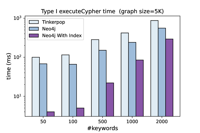
(a) Graph size $=5K$.

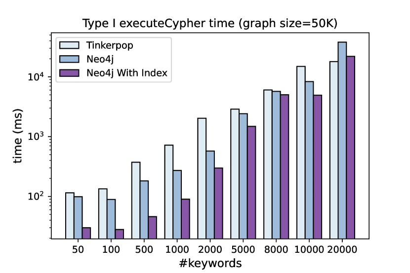
(b) Graph size $=50K$.

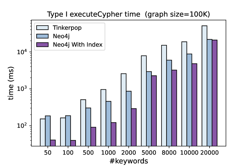
(c) Graph size $=100K$.

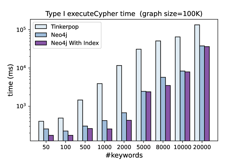
(d) Graph size $=500K$.

Figure 17. Calibration results for Type I Cypher query w.r.t. different graph sizes and #keywords.

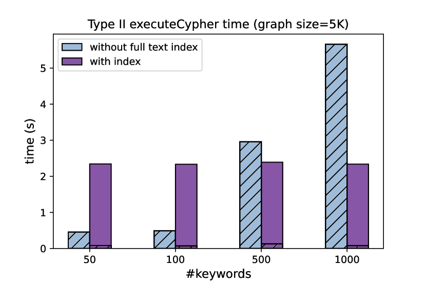
(a) Graph size $=5K$.

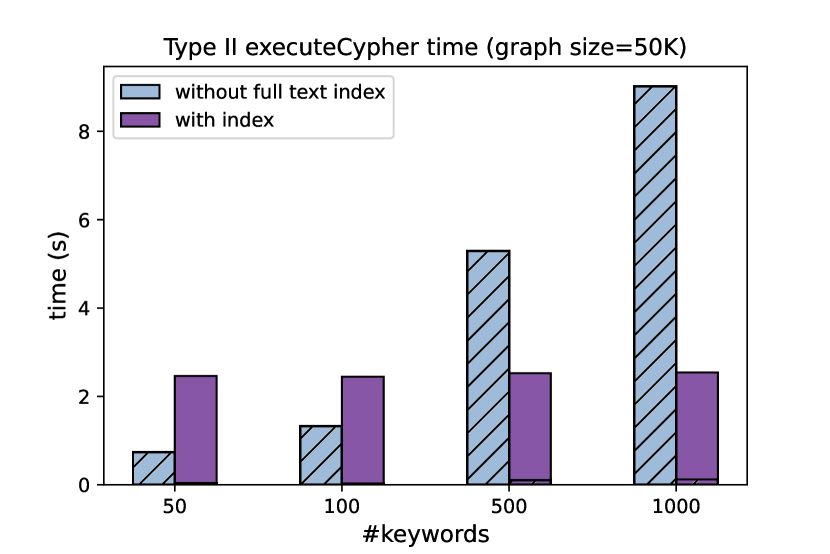
(b) Graph size $=50K$.

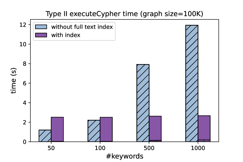
(c) Graph size $=100K$.

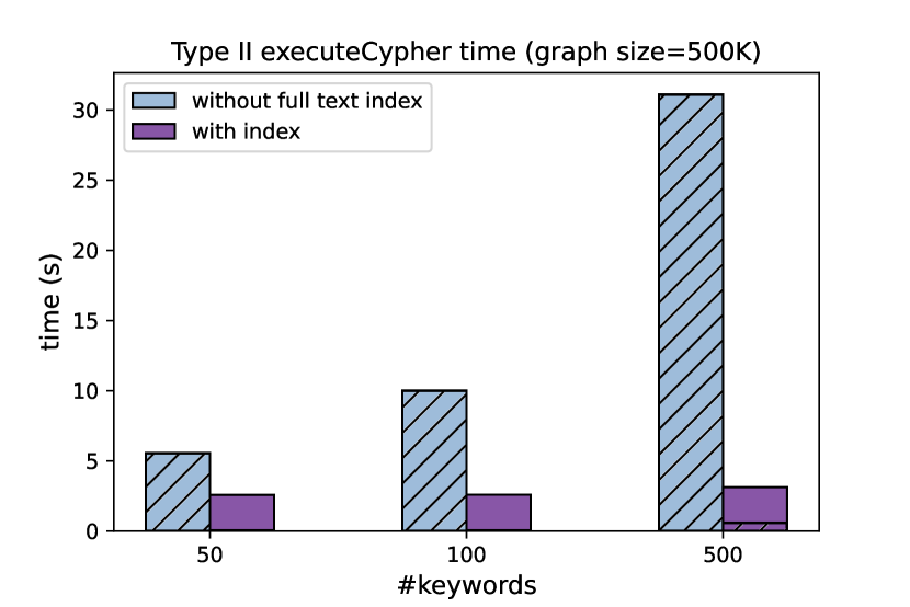
(d) Graph size $=500K$.

Figure 18. Calibration results for Type II Cypher query w.r.t. different graph sizes and #keywords.

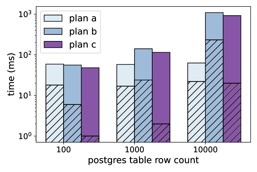
(a) Row count of R: 100.

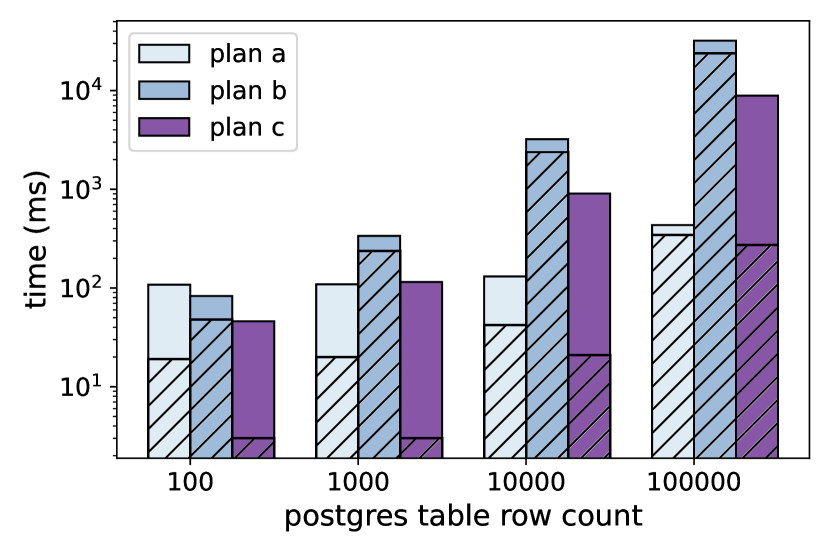
(b) Row count of R: 1K.

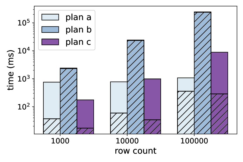
(c) Row count of R: 10K.

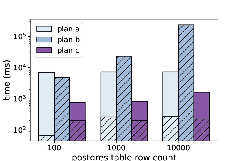
(d) Row count of R: 100K.

Figure 19. Calibration results for cross engine executeSQL

Appendix E AWESOME logical and physical operators.

Table 6. AWESOME logical and physical operators.

Types	Logical Operators	Physical Operators	DataParallelCap	BufferingCap
Query	ExecuteCypher ExecuteSQL ExecuteSolr	ExecuteCypherInNeo4j ExecuteCypherInMeomory ExecuteSQLInPostgres ExecuteSQLInSQLite ExecuteSolr FetchDBMSResults	ST ST ST ST ST ST	B B B B B SO
Graph Operations	BuildWordNeighborGraph BuildGraphFromRelation BuildGraph PageRank ComputeNodeDegrees ComputeKNeighbors	CollectGraphElementsFromDocs CollectGraphElementsFromRelation CreateNeo4jGraph CreateInMemoryGraph PageRankInNeo4j PageRankInMemory ComputeNodeDegrees ComputeKNeighbors	PR PR ST ST ST ST PR PR	SS SS SI SI SO SO SO SO
Relation Operations	GetColumns	GetColumns RecordsToList	ST ST	SS SS
Text Operations	Tokenize LDA SVD TopicModel PhraseExtraction NER	CreatDocumentsFromRecord CreatDocumentsFromList FilterStopWords SplitByPatterns CreateTextMatrix PhraseExtraction NER LDA SVD	PR PR PR PR ST PR PR ST ST	SS SS SS SS SI SS SS B B
MappedMatrix Operations	TopicModel GetValue ColumnKeys RowKeys	LDA SVD GetValueByIndex GetValueByKeys ColumnKeys RowKeys	ST ST ST ST ST ST	B B B B B B
Other Functions	Sum Range	SumList SumColumn SumMatrix SumVector Range	PR PR PR PR ST	SI SI SI SI SO
Data Movement	Store	ListToPostgres InMemoryRelationToPostgres InMemoryGraphToNeo4j RecordsToPostgres GraphElementsToNeo4j ListToCSV InMemoryRelationToCSV RecordsToCSV	ST ST ST ST ST ST ST ST	SI B B SI SI SI B SI