Observational constraints on Starobinsky $f(R)$ cosmology from cosmic expansion and structure growth data

Abstract

The unknown physical nature of the Dark Energy motivates in cosmology the study of modifications of the gravity theory at large distances. One of these types of modifications is to consider gravity theories, generally termed as $f(R)$. In this paper we use observational data to both constrain and test the Starobinsky $f(R)$ model Starobinsky2007 , using updated measurements from the dynamics of the expansion of the universe, $H(z)$; and the growth rate of cosmic structures, $[f\sigma_{8}](z)$, where the distinction between the concordance $\Lambda$CDM model and modified gravity models $f(R)$ becomes clearer. We use MCMC likelihood analyses to explore the parameters space of the $f(R)$ model using $H(z)$ and $[f\sigma_{8}](z)$ data, both individually and jointly, and further, examine which of the models best fits the joint data. To further test the Starobinsky model, we use a method proposed by Linder Linder2017 , where the data from the observables is jointly binned in redshift space. This allows to further explore the model’s parameter that better fits the data in comparison to the $\Lambda$CDM model. The joint analysis of $H(z)$ and $[f\sigma_{8}](z)$ show that the $n=2$–Starobinsky $f(R)$ model fits well the observational data. In the end, we confirm that this joint analysis is able to break the degenerescence between modified gravity models as proposed in the original work Starobinsky2007 . Our results indicate that the $f(R)$ Starobinsky model provides a good fit to the currently available data for a set of values of its parameters, being, therefore, a possible alternative to the $\Lambda$CDM model.

1 Introduction

The search for an explanation to the current phase of accelerated expansion of the universe is one of the most important paradigms in modern cosmology Planck:2015bue . With the available observational information, the concordance model of cosmology that best fits the data is the flat $\Lambda$CDM Planck2018 model, where the universe is filled in with cold dark matter (CDM) and a dark energy (DE) component –in the form of a cosmological constant $\Lambda$– in addition to the standard baryonic and electromagnetic ingredients. The main concern with the DE is that its physical interpretation is still unknown. Other plausible causes of the observed accelerated expansion should be explored Kazantzidis:2018rnb ; Basilakos_2020 ; Linder_2020 ; Velasquez_Toribio_2020 ; Bonilla_2021 ; Davari_2021 . Because $\Lambda$CDM is based on Einstein’s general relativity (GR), one possible way is to explore cosmological models not based on GR Linder ; Benaoum ; Perenon15 ; Perenon19 ; Perenon20 ; Batista14 ; Nunes18 ; Benisty18 ; Benisty19a ; Benisty19b . However, there is a degeneracy problem between models supported by GR and models based on other metric theories, generally termed Modified Gravity (MG) theories. This degenerescence cannot be broken using data from the dynamical evolution of the Universe alone, as the same dynamics can be explained by different MG theories as well as by evolving DE fluids, $\omega=\omega(a)$, where $a$ is the scale factor Hu2007 ; Clifton2011 ; Martinelli2011 . The best observable to discriminate between MG theories and $\Lambda$CDM is the growth rate of cosmic structures, $f(a)$, defined as Strauss

$$f(a)\equiv\dfrac{d\ln\delta}{d\ln a}\,,$$ (1)

where $\delta$ is the matter density contrast. The growth rate $f=f(a)$ has indeed the potential to constrain models based on MG theories and $\Lambda$CDM DE (based on GR) from the measure of the growth index, $\gamma$, when one parametrizes $f$ as Linder

$$f(a)=\Omega_{m}(a)^{\gamma}\,.$$ (2)

In the $\Lambda$CDM concordance model, $\gamma\simeq 0.55$, and for some MG models $\gamma$ evolves with time: $\gamma\simeq 0.41-0.21z$ Basilakos12 . In fact, changing the gravitational theory will affect the way how matter clumps at all scales, beyond the expansion of the homogeneous universe. As such, alternative cosmological models based on MG theories make very different predictions for matter clustering and evolution.

Direct measurements of $f(a)$, or equivalently of $f(z)$, where the scale factor and the redshift are related by $a=1/(1+z)$, are difficult to obtain. Instead the data available comes from the measurements of the galaxy redshift space distortions in the form of a product of two quantities evolving with time: $[f\sigma_{8}](z)\equiv f(z)\sigma_{8}(z)$, where $\sigma_{8}$ is the root-mean-square linear fluctuation of the matter distribution at the scale of 8 Mpc$/h$, $h$ the dimensionless Hubble parameter, where $H_{0}=100\,h$ km/s/Mpc. Notice that the letter $f$ refers to the growth rate of cosmic structures, that is, it represents the function $f(a)$ or $f(z)$, but it is commonly used in the form $f(R)$ to refer to MG theories. In what follows the symbol $f(R)$, as a function of $R$, only refers to MG theories, while the letter $f$ alone or the function $f(a)$, or $f(z)$, refers to the cosmic growth rate. In this paper, we use this observational parameter, $[f\sigma_{8}]$ and the background evolution of the universe, $H$ to explore the parameter space and test a model of $f(R)$ gravity, namely, the Starobinsky $f(R)$ model.

We use a Markov Chain Monte Carlo (MCMC) method to explore the parameter space of the theory with the selected datasets for $H(z)$ and $[f\sigma_{8}](z)$, both individually and jointly. In the end, we further extend our analysis with a joint study of the observables proposed by Linder Linder2017 and, in the context of Modified Gravity, more recently by Matsumoto Matsumoto2020 .

This work is organized as follows. A brief description of the Starobinsky cosmological model Starobinsky2007 is presented in section 2. In section 3 we provide details of the two data sets used in the analyses, and in section 4 we describe the methodology of the analyses performed, show our results, and provide their statistical interpretation. The conclusions obtained from these analyses and the final remarks of our work are addressed in section 5.

2 Starobinsky f(R) model cosmology

2.1 Background space-time

A general $f(R)$ theory in the metric formalism that is minimally coupled to matter has an action DeFelice2010

$$S=\int d^{4}x\sqrt{-g}\left[\frac{1}{2\kappa}f(R)+\mathcal{L}_{m}(g_{\mu\nu})\right],$$ (3)

where we include in the action the matter Lagrangian density, $\mathcal{L}_{m}$, and define $\kappa\equiv 8\pi G$ (we adopt units with $c=1$). This allows us to use geometrized units more easily when needed. In this work we define the function $f(R)$ as in the model introduced by Starobinsky Starobinsky2007

$$f(R)\equiv R+\lambda R_{0}\left(\left(1+\frac{R^{2}}{R_{0}^{2}}\right)^{-n}-1\right).$$ (4)

$R_{0}$ and $\lambda$ are model parameters related to the observed DE density and a characteristic curvature, respectively Chen2019 , which can be constrained by the measured cosmological parameters using equation (2.1). In this paper we will analyse the cases $n=1$ and $n=2$, which are extensively studied in the literature Kopp_2013 ; Chen2019 . While the model with $n=1$ is known to have difficulty in passing solar system tests and reproducing the matter density fluctuations power spectrum Starobinsky2007 ; MOTOHASHI_2009 , it is still used in the literature as a prototypical example of the theory, as well as a fit to the data and MCMC analysis Chen2019 ; Cardone2012 ; Hough2020 . The parameter range for models which pass the Solar System test is $n\geq 2$, which also has the most pronounced effect on the evolution of matter perturbations Motohashi_2013 ; Chudaykin_2015 .

The variation with respect to the metric gives rise to the field equations of this model, given by the extended Einstein equations

$$F(R)R_{\mu\nu}-\frac{1}{2}f(R)g_{\mu\nu}-[\nabla_{\mu}\nabla_{\nu}-g_{\mu\nu}\square]F(R)=\kappa T_{\mu\nu},$$ (5)

$$F(R)R-2f(R)+3\,\square f(R)=\kappa T,$$ (6)

where we define $F(R)\equiv d\/f(R)/dR$, $T\equiv g^{\mu\nu}T_{\mu\nu}$, and the second equation is the trace of the first one, useful to derive the dynamics of the $f(R)$ function, which is more complicated than in GR where one has an algebraic relation between $R$ and $T$ Sotiriou2010 .

To model our cosmological space-time we adopt the Friedmann-Lemaître-Robertson-Walker (FLRW) for the background space-time filled with a perfect fluid, with metric and stress-energy tensor given by, respectively,

$$ds^{2}=-dt^{2}+a^{2}(t)\left[\frac{dr^{2}}{1-Kr^{2}}+r^{2}(d\theta^{2}+\sin^{2}\theta\,d\phi^{2})\right],$$ (7)

$$T^{\mu\nu}=(\rho+P)u^{\mu}u^{\nu}+Pg^{\mu\nu},$$ (8)

where we take, as usual, $K$ is the scalar curvature of the 3-space, and $\rho$ and $P$, are the density and pressure of the perfect fluid, respectively. $u^{\mu}$ is the 4-velocity vector of an observer comoving with the fluid; $a=a(t)$ is the dimensionless scale factor, with $a(t_{0})=1$, $t_{0}$ is today’s cosmic time, and we always use geometrized units, unless otherwise noted. Because we shall compare our analyses with those of the flat $\Lambda$CDM model, we consider the flat FLRW space-time, i.e., $K=0$.

One can analyse the dynamical evolution of our cosmological model using equations (7) and (8) in equation (6), obtaining the modified Friedmann equations

$$\!H^{2}=\frac{\kappa}{3F(R)}\left[\rho+\frac{RF(R)-f(R)}{2}-3H\dot{R}F^{\prime}(R)\right],$$ (9)

$$2\dot{H}+3H^{2}=-\frac{\kappa}{F(R)}\left[P+\dot{R}^{2}F^{\prime\prime}(R)+2H\dot{R}F^{\prime}(R)\right.$$

$$\hskip 56.9055pt+\,\ddot{R}F^{\prime}(R)+\frac{1}{2}(f(R)-RF(R))\Big{]},$$ (10)

where $\dot{\,}$ means derivative with respect to the cosmic time $t$. These equations must obey certain constraints in order that our model is stable and correctly reproduces the late-time acceleration of the universe, without deviating from $\Lambda$CDM at early times (associated with $R\gg R_{0}$). An analysis of such constraints on general $f(R)$ theories can be found in Sotiriou2010 . Following Starobinsky2007 , it suffices that (4) should satisfy, for the values $n=1$ and $n=2$

$$F(R)>0\,,\quad F^{\prime}(R)>0\,,\quad R\geq R_{1}\,,\quad\lambda>\frac{8\sqrt{3}}{3}\,,\quad n=1,$$ (11)

$$\lambda>\frac{\sqrt{(\sqrt{13}-2)}}{2}\,,\quad n=2$$ (12)

where $R_{1}$ is the Ricci curvature of a de Sitter point in the space of solutions. More stringent constraints on the model parameters $n$ and $R_{1}$, can be obtained by likelihood analyses on various data sets for the Starobinsky and other $f(R)$ models, like the ones performed in ref. Cardone2012 , whereas more extensive and general analyses of the stability of the model can be found in ref. Motohashi_2011_1 .

It will be convenient to write equation (4) in terms of the measured cosmological parameters $\Omega_{m0}=\frac{8\pi G\rho_{m0}}{3H_{0}^{2}}$ and $\Omega_{\Lambda 0}=\frac{8\pi G\rho_{\Lambda}}{3H_{0}^{2}}$. In this case, one can find the correct way to write the parameters by making the model return to $\Lambda$CDM at high $z$ limit Starobinsky2007 ; Chen2019

$$f(R)=\,\, R\,+\,6\lambda H_{0}^{2}(1-\Omega_{m})$$

$$\times\left(\left(1+\frac{R^{2}}{[6H_{0}^{2}(1-\Omega_{m})]^{2}}\right)^{-n}-1\right)\,.$$ (13)

This relation allows us to constrain $R_{0}$ and $\lambda$ using data linked to the observables $\Omega_{m0}$ and $H_{0}$.

2.2 Metric perturbations

In order to go beyond the background cosmological observables and test our theory against structure growth we need to introduce metric perturbations. Following the general perturbative procedure for scalar-tensor theories found in Tsujikawa2007 , in the usual Newtonian (or comoving) gauge, the perturbed metric is given by

$$ds^{2}=-(1+2\Psi)\/dt^{2}+(1-2\Phi)\,a^{2}(t)\,\delta_{ij}dx^{i}dx^{j}\,,$$ (14)

where $i,j=1,2,3$, and $\Psi,\Phi$ are the Bardeen potentials which satisfy $\Psi=\Phi$ in the absence of anisotropic stress. The physical processes we are interested in, and the cosmological observables associated with them (i.e., accelerated cosmic expansion and growth of cosmic structures), are all well within the scale of the sub-horizon approximation $k\gg a^{2}H^{2}$. In this case, we can write the evolution equation for the matter density contrast, $\delta$, as

$$\ddot{\delta}+2H\dot{\delta}+\frac{k^{2}}{a^{2}}\Phi=4\pi G\,\mu(k,a)\,\rho_{m}\,\delta\,,$$ (15)

where $G$ is the Newtonian gravitational constant. The $\mu(k,a)$ factor is written as

$$\mu(k,a)\equiv\frac{1}{8\pi F(R)}\left(\frac{1+4\frac{k^{2}}{a^{2}R}\,m}{1+3\frac{k^{2}}{a^{2}R}\,m}\right),$$ (16)

where $m$ is a parameter that quantifies the deviation from the $\Lambda$CDM model

$$m\equiv\frac{RF^{\prime}(R)}{F(R)}\implies m|_{{\footnotesize\Lambda CDM}}=0\,.$$

Equation (15) allow us to analyse how our cosmological model should behave at the limits of very small and very large scales; since $R$ is of the order of $H(z)$, we obtain

$$\lim_{k\gg a^{2}H^{2}}\mu(k)=\frac{4}{3}\,\frac{1}{8\pi F(R)},$$ (17)

$$\lim_{k\ll a^{2}H^{2}}\mu(k)=\frac{1}{8\pi F(R)}\,,$$ (18)

and we observe that, at small scales, the modification of GR gives an extra factor of $\frac{4}{3}$ to the force term of the equation, therefore gravity becomes stronger and cosmic structures grow faster. In the opposite limit, at large scales, the equation (15) is the same as in GR Tsujikawa2007 , now with the term $1/F(R)$, which arises naturally in a theory that couples to gravity. In the language of the Scalar-Tensor theory, this would be the term that couples gravity to the scalar field.

The regime of cosmic structure formation lies between these scales, so that we need the full equation (15) to account for the physics in this regime. However, when the Hubble scale is not large enough in comparison to the perturbations (high redshift), or when we have scales of the order of $H_{0}$ (low redshift), the behavior of the structure formation should have the $\Lambda$CDM model as a limit.

It is useful to rewrite equation (15) as an ODE on the variable $N\equiv\ln{a}$, also called the e-fold number, which can be obtained after a simple chain rule derivation

$$\delta^{\prime\prime}+\left(2+\frac{H^{\prime}}{H}\right)\delta^{\prime}-\frac{3}{2}\Omega_{m}(a)\,\mu(k,a)\,\delta=0\,,$$ (19)

where ^′ means derivative with respect to $N$, and $\Omega_{m}(a)$ is the density parameter of (dark + baryonic) matter as a function of the scale factor $a$, defined above. This is the equation to be solved in order to find the linear growth of our model, using the definition of the growth rate of cosmic structures function $f(a)$ given in equation (1) in the same way as in GR.

3 Observational Data

There are in the literature several compilations of $H(z)$ and $[f\sigma_{8}](z)$ observational data. In this section, we are going to present the datasets we are considering to impose observational constraints in the Starobinsky model.

3.1 H(z) data

The history of the expansion of the universe is probed by the observational Hubble parameter $H(z)$. It can be measured by several independent methodologies, most of them, based on distance measurements of galactic objects such as supernovae and quasars. However, it is known that in some approaches the cosmological distance measurements depend on a fiducial model, which makes the use of these data problematic when the objective is to constrain the free parameters of cosmological models in alternative scenarios.

In this work, since we are considering a gravity model of type $f(R)$, we are going to use in our analyses, the $H(z)$ measurements obtained by the differential age technique, which is independent of the fiducial model. This technique, also known as cosmic chronometers (CC), was proposed by Jimenez and Loeb in Jimenez_2002 .

The basic idea of the CC data consists of the spectroscopic determination of the age difference between two passively evolving early-type galaxies. The assumption of old galaxies to realize the age difference measurements is important to assure that the galaxies were formed at the same time, although are localized in slightly different redshift.

The Hubble parameter is directly related to the measured quantity $dz/dt$ by

$$H(z)=-\frac{dz}{dt}\frac{1}{(1+z)}\,.$$ (20)

In this work we use the compilation of $31$ measurements of $H(z)$, covering the range $0.07<z<1.965$ Yang_2020 . The data is shown in Table 1 and in Fig. 1.

Table 1: The $31$ Hubble parameter data points, $H(z)$, and their respective $1\,\sigma$ errors $\sigma_{H}(z)$ from the CC data Yang_2020 . The units for both $H(z),\sigma_{H}(z)$ are km/s/Mpc.

$z$	$H(z)$	$\sigma_{H}(z)$
0.07	69.0	19.6
0.09	69.0	12.0
0.12	68.6	26.2
0.17	83.0	8.0
0.179	75.0	4.0
0.199	75.0	5.0
0.2	72.9	29.6
0.27	77.0	14.0
0.28	88.8	36.6
0.352	83.0	14.0
0.3802	83.0	13.5
0.4	95.0	17.0
0.4004	77.0	10.2
0.4247	87.1	11.2
0.4497	92.8	12.9
0.47	89.0	49.6
0.4783	80.9	9.0
0.48	97.0	62.0
0.593	104.0	13.0
0.68	92.0	8.0
0.781	105.0	12.0
0.875	125.0	17.0
0.88	90.0	40.0
0.9	117.0	23.0
1.037	154.0	20.0
1.3	168.0	17.0
1.363	160.0	33.6
1.43	177.0	18.0
1.53	140.0	14.0
1.75	202.0	40.0
1.965	186.5	50.4

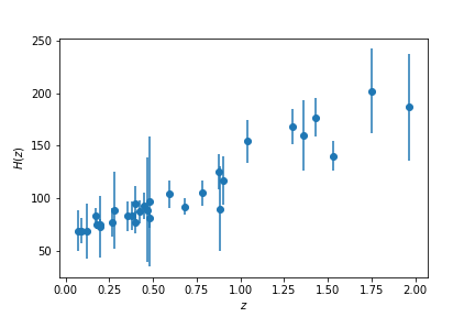
Figure 1: The CC Hubble parameter data, $H(z)$, displayed in Table 1.

3.2 $[f\sigma_{8}](z)$ data

Precise measurements of $[f\sigma_{8}](z)$ can be done using the Redshift Space Distortions (RSD) approach, by studying the peculiar velocities caused by local gravitational potentials that introduce distortions in the two-point correlation function of cosmic objects 1987MNRAS.227….1K . In fact, the calculation of the anisotropic two-point correlation function, $\xi(s,\mu)$ Hamilton1992ApJ , allows us to measure $f\sigma_{8}$, where $\sigma_{8}$ is the root-mean-square linear fluctuation of the matter distribution at the scale of 8 Mpc$/h$ (for other approaches to study matter clustering see, e.g., Avila19 ; Marques20 ; deCarvalho18 ; deCarvalho20 ). The literature reports diverse compilations of measurements of $[f\sigma_{8}](z)$ (see, e.g., Nunes:2015xsa ; Alam21 ) which we update here. Our compilation, shown in Table 2 and in Fig. 2, takes into account:

1. we consider $[f\sigma_{8}](z)$ data obtained from disjoint or uncorrelated redshift bins when the measurements concern the same cosmological tracer, and data from possibly correlated redshift bins when different cosmological tracers were analyzed;

2. we consider the latest measurement of $[f\sigma_{8}](z)$ when the same survey collaboration performed two or more measurements corresponding to several data releases.

Table 2: Updated compilation of 26 $[f\sigma_{8}](z)$ data with their respective $1\sigma$ errors, $\sigma_{f\sigma_{8}}$.

Survey	$z$	$[f\sigma_{8}]\pm\sigma_{f\sigma_{8}}$	Reference	Cosmological tracer
ALFALFA	0.013	$0.46\pm 0.06$	Avila21a	HI line sources
SNIa+IRAS	0.02	$0.398\pm 0.065$	Turnbull	galaxies+SNIa
SNIa+6dFGS	0.02	$0.428\pm 0.0465$	Huterer	galaxies+SNIa
6dFGS	0.025	$0.39\pm 0.11$	Achitouv17	voids
6dFGS	0.067	$0.423\pm 0.055$	Beutler	galaxies
SDSS-veloc	0.10	$0.370\pm 0.130$	Feix	galaxies
SDSS-IV	0.15	$0.53\pm 0.16$	Alam21	MGS
BOSS-LOWZ	0.32	$0.384\pm 0.095$	Sanchez	LOWZ and CMASS samples
SDSS-IV	0.38	$0.500\pm 0.047$	Alam21	BOSS galaxy sample
WiggleZ	0.44	$0.413\pm 0.080$	Blake12	ELG
BOSS-CMASS	0.57	$0.453\pm 0.022$	Nadathur	voids+galaxies
SDSS-CMASS	0.59	$0.488\pm 0.060$	Chuang16	CMASS galaxy sample
VIPERS PDR-2	0.60	$0.550\pm 0.120$	Pezzotta17	galaxies
SDSS-IV	0.70	$0.448\pm 0.043$	Alam21	eBOSS DR16 LRG
WiggleZ	0.73	$0.437\pm 0.072$	Blake12	ELG
SDSS-IV	0.74	$0.50\pm 0.11$	Aubert20	eBOSS DR16 Voids
Vipers v7	0.76	$0.440\pm 0.040$	Wilson	galaxies
SDSS-IV	0.85	$0.52\pm 0.10$	Aubert20	eBOSS DR16 Voids
SDSS-IV	0.85	$0.315\pm 0.095$	Alam21	eBOSS DR16 ELG
VIPERS PDR-2	0.86	$0.400\pm 0.110$	Pezzotta17	galaxies
SDSS-IV	0.978	$0.379\pm 0.176$	Zhao	eBOSS DR14 Quasar
Vipers v7	1.05	$0.280\pm 0.080$	Wilson	galaxies
FastSound	1.40	$0.482\pm 0.116$	Okumura	ELG
SDSS-IV	1.48	$0.30\pm 0.13$	Aubert20	eBOSS DR16 Voids
SDSS-IV	1.48	$0.462\pm 0.045$	Alam21	eBOSS DR16 Quasar
SDSS-IV	1.944	$0.364\pm 0.106$	Zhao	eBOSS DR14 Quasar

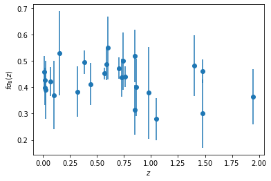
Figure 2: The $[f\sigma_{8}](z)$ data displayed in Table 2.

3.3 Joint data

The binned data given in Table 3 was obtained binning simultaneously the $[f\sigma_{8}](z)$ and $H(z)$ (from the Table 2 and the Table 1, respectively) in $5$ redshift bins: $(0.0,0.30]$,  $(0.30,0.60]$,  $(0.60,0.85]$,  $(0.85,1.4]$,  $(1.4,2.0]$, with mean redshifts: $\bar{z}=\,0.15,\,0.45,\,0.725,\,1.125,\,1.7$. The number of data pairs $(f\sigma_{8},H)$ in each bin were: $(7,9)$, $(6,10)$, $(6,2)$, $(4,6)$, $(3,4)$, respectively. The values in these $5$ bins for $[f\sigma_{8}](z)$ and $H(z)$, and their errors, correspond to their variance weighted means Moresco2017 . This binned data will be used in the $\chi^{2}$ joint analysis.

Table 3: Binned data of $[f\sigma_{8}](z)$ and $H(z)$ obtained by calculating the variance weighted mean in each redshift bin (see the text for details).

$\bar{z}$	$[f\sigma_{8}](z)$	$H(z)$
0.15	$0.4284\pm 0.0338$	$75.367\pm 5.741$
0.45	$0.4647\pm 0.0288$	$88.880\pm 6.717$
0.725	$0.4433\pm 0.0313$	$98.500\pm 7.071$
1.125	$0.3852\pm 0.0602$	$135.667\pm 10.247$
1.70	$0.3753\pm 0.0541$	$176.375\pm 15.300$

4 Analyses and Results

In this section we describe the parameter space analyses of the $f(R)$ model given in equation (4), using the observational data described in the previous section 3. To obtain the theoretical predictions for $H(z)$ and $f(z)$ from the chosen model, equation (3), we integrate equations (9) and (19) numerically and use their results in the assembling of the likelihood function. This gives us our statistical analyses.

The standard Bayesian inference will be considered for the parameter estimation. To investigate how appropriate the data is to constrain the parameter space of the model, they will be considered separately and later combined in a joint analysis.

4.1 $H(z)$ and $[f\sigma_{8}](z)$ observational constraints

Recently, the tension between different estimates of the Hubble constant has drawn the attention of cosmologists. The local determination of the Hubble constant from SHO-ES collaboration Riess:2019cxk is $H_{0}^{\mbox{\tiny SHOES}}=74.03\pm 1.42$ km/s/Mpc while the value inferred by the Planck collaboration Planck2018 , from the Cosmic Microwave Background (CMB) analysis in a flat $\Lambda$CDM framework is $H_{0}^{\mbox{\tiny Planck}}=67.36\pm 0.54$ km/s/Mpc from the last Planck collaboration results Planck2018 .

The divergence in $H_{0}$ measurements is the main reason to look for alternative approaches to perform analyses that are independent of the $H_{0}$ value NB20 . In our analyses, we shall consider $H(z)/H_{0}$ instead of $H(z)$ data, and for this we use $H_{0}=H_{0}^{\mbox{\tiny Planck}}$ Planck2018 .

For the model given in equation ((4)) and $H(z)$ data, the Likelihood function is given by

$$\mathcal{L}(z|\theta)\propto-\frac{1}{2}\sum_{i}^{N_{H}}\,\frac{(H^{i}_{th}(z|\theta)-H^{i}_{obs}(z))^{2}}{\sigma_{i}^{2}}\,,$$ (21)

where $N_{H}$ is the number of points in the dataset, $\theta={(\Omega_{m0},\lambda)}$ are the free parameters of the model, $H^{i}_{th}(z|\theta)$ is the theoretical Hubble parameter at redshift $z_{i}$, $H^{i}_{obs}(z)$ and $\sigma$ are the observation error values of the Hubble parameter given in table 1.

The theoretical Hubble parameter depends on the current Hubble parameter $H_{0}$. To eliminate this dependency, we will follow the approach introduced by Anagnostopoulos , that consists of marginalization of the likelihood over $H_{0}$ parameters

$$\mathcal{L}=\Gamma-\frac{B^{2}}{A}+\ln{A}-2\ln{\left[1+\textrm{erf}\left(\frac{B}{\sqrt{2A}}\right)\right]}\,,$$ (22)

where, by the definition of $E(z)\equiv H_{th}/H_{0}$,

$$A=\sum^{N}_{i=1}\frac{E^{2}(z_{i})}{\sigma_{i}^{2}}\,,$$ (23)

$$B=\sum^{N}_{i=1}\frac{E(z_{i})H_{obs}(z_{i})}{\sigma_{i}^{2}}\,,$$ (24)

and

$$\Gamma=\sum^{N}_{i=1}\frac{H_{obs}^{2}(z_{i})}{\sigma_{i}^{2}}\,.$$ (25)

Similarly, the Likelihood function for $[f\sigma_{8}](z)$ data is given by:

$$\mathcal{L}(z|\theta)\propto-\frac{1}{2}\sum_{i}^{N_{f}}\,\frac{(f\sigma_{8}^{i_{th}}(z|\theta)-f\sigma_{8}^{i_{obs}}(z))^{2}}{\sigma_{i}^{2}}\,,$$ (26)

where we have the same parametric space $\theta={(\Omega_{m0},\lambda)}$, $f\sigma_{8}^{i_{th}}(z|\theta)$ is the theoretical growth function given by the model with parameters $\theta$ at redshift $z_{i}$; $f^{i}_{obs}(z)$ and $\sigma$ are the observed values, given by the data in Table 2; $N_{f}$ is the size of the $f\sigma_{8}$ dataset. The $f\sigma_{8}$ function does not have $H_{0}$ as a free parameter and therefore does not need to be marginalized. The parametric space of both observables $H(z)$ and $[f\sigma_{8}](z)$ are the same and the joint likelihood function is given by the product of the individual likelihoods according to

$$\mathcal{L}=\mathcal{L}_{H}\times\mathcal{L}_{f\sigma_{8}}.$$ (27)

The Bayesian inference of the parameters is obtained through the expected values of the posterior density $p(\theta|z)$ and since the posteriori distribution is unknown for the model, i.e., it can not be approximated by a normal or gaussian distribution, we are considering the Bayes Theorem that establishes

$$p(\theta|z)=\mathcal{L}(z|\theta)\times\Pi(\theta)$$ (28)

where $\Pi(\theta)$ is the prior.

The parametric space of the variables of the model will be explored following the methodology of Markov chain Monte Carlo (MCMC) and the Metropolis–Hastings algorithm to generate a set of samples from a posteriori distribution. To implement the MCMC, we are using a Python open-source code, emcee Foreman_Mackey_2013

The posteriori distribution was generated for the following intervals in the $n=1$ case, with flat distributions: $\lambda^{-1}\in[0.001,1.8]$ and $\Omega_{m0}\in[0.2,0.6]$ for the $H(z)$ data set; $\lambda^{-1}\in[0.001,2.0]$ and $\Omega_{m0}\in[0.15,0.3]$ for the $[f{\sigma 8}](z)$ data set; and finally, $\lambda^{-1}\in[0.001,2.0]$ and $\Omega_{m0}\in[0.2,0.4]$ for the combined data set. For the $n=2$ case we use a flat prior in all the MCMC runs, as well, we consider the same intervals $\lambda^{-1}\in[0.1,2]$, $\Omega_{m0}\in[0.15,0.4]$.

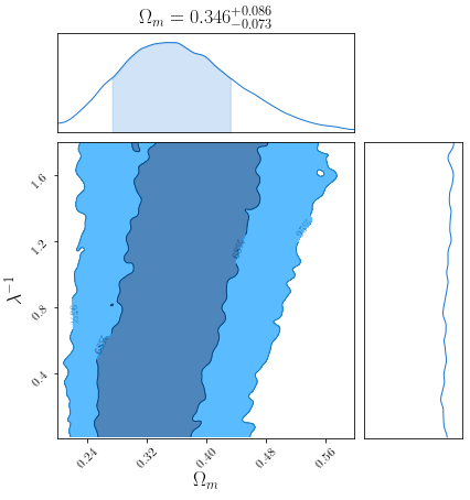
Figure 3: MCMC simulations for the $f(R)$ model with $n=1$, considering $H(z)$ data and the flat priors: $\lambda^{-1}=[0.001,1.8]$ and $\Omega_{m0}=[0.2,0.6]$.

.

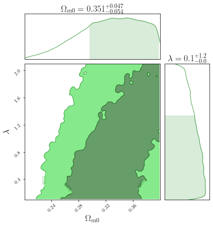
Figure 4: MCMC simulations for the $f(R)$ model with $n=2$, considering $H(z)$ data and the flat priors: $\lambda^{-1}\in[0.1,2]$ and $\Omega_{m0}\in[0.15,0.4]$.

.

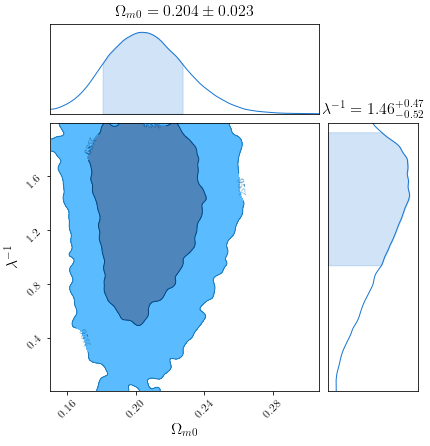
Figure 5: MCMC simulations for the $f(R)$ model with $n=1$, considering $[f\sigma_{8}](z)$ data and the flat priors: $\lambda^{-1}\in[0.001,2.0]$ and $\Omega_{m0}\in[0.15,0.3]$.

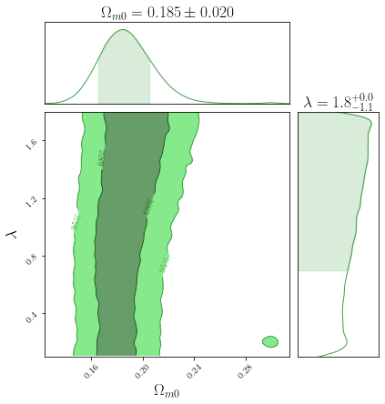
Figure 6: MCMC simulations for the $f(R)$ model with $n=2$, considering $[f\sigma_{8}](z)$ data and the flat priors: $\lambda^{-1}\in[0.1,2.0]$ and $\Omega_{m0}\in[0.15,0.4]$.

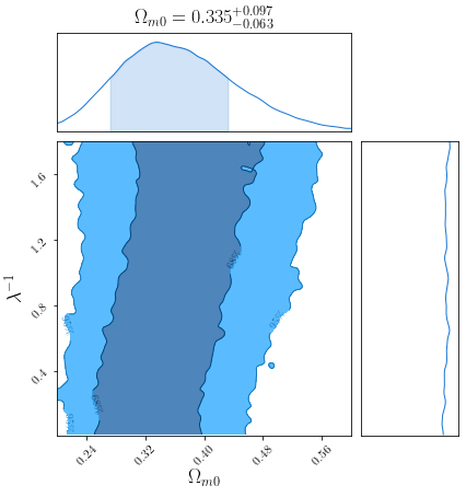
Figure 7: MCMC simulations for the $f(R)$ model with $n=1$, considering joint analyses of the $H(z)$ and $[f\sigma_{8}](z)$ data and the flat priors: $\lambda^{-1}=[0.001,2.0]$ and $\Omega_{m0}=[0.2,0.4]$.

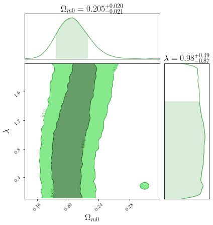
Figure 8: MCMC simulations for the $f(R)$ model with $n=2$, considering joint analyses of the $H(z)$ and $[f\sigma_{8}](z)$ data and the flat priors: $\lambda^{-1}=[0.1,2.0]$ and $\Omega_{m0}=[0.15,0.4]$.

We summarize our results in Table 4, and the parameter space contours obtained can be seen in blue in figures 3, 5, and 7 for the $n=1$ case; and in green in figures 4, 6, and 8 for the $n=2$ case.

Data	Model	$\Omega_{m0}$	$\lambda^{-1}$
$H$	n=1	$0.346^{+0.086}_{-0.073}$	$1.1936$ (unconstrained)
$f\sigma_{8}$	n=1	$0.204{\pm}0.023$	$1.460^{+0.47}_{-0.52}$
$H+f\sigma_{8}$	n=1	$0.335^{+0.097}_{-0.063}$	$1.761$ (unconstrained)
$H$	n=2	$0.351^{+0.049}_{-0.051}$	$0.38^{+0.98}_{-0.28}$
$f\sigma_{8}$	n=2	$0.185{\pm}0.020$	$1.8^{+0.00}_{-1.1}$
$H+f\sigma_{8}$	n=2	$0.205{\pm}0.020$	$0.99^{+0.72}_{-0.65}$

Table 4: Results of our likelihood analyses for the cosmological parameters and their uncertainties.

4.2 $[f\sigma_{8}-H]$ diagram analyses

Recently, Linder Linder2017 and Matsumoto et al. Matsumoto2020 have proposed a joint analysis of the $H(z)$ and $[f\sigma_{8}](z)$ cosmological observables as a way to break the degeneracy of DE and MG models, also allowing to recognize the redshift regime where the tested model most affects the growth of cosmic structures.

In Moresco et al. Moresco2017 , the authors used a joint statistical analysis of both these observables and applied the method of Linder Linder2017 to analyze individually the parameters of $\Lambda$CDM + $\Sigma m_{\nu}$ and $w$CDM (for cosmological parameter analyses with massive neutrinos see, e.g., Marques19 ). The authors obtained $1\sigma$ constraints on the parameters from growth structure data at low redshifts ($z<2$) and the last Planck (2018) data release. Of particular interest was the degeneracy between models with massive neutrinos and a modified growth parameter $\gamma$, according to this analysis the models investigated provide a better fit than the flat $\Lambda$CDM model, as constrained by the Planck mission Planck2016 . The authors then simulated data points in the $f\sigma_{8}-H$ plane to distinguish between the models that better fit the data, and found that they could be distinguished with high statistical significance using the $f\sigma_{8}-H$ plane. This shows that the joint analysis proposed by Linder Linder2017 and Matsumoto et al. Matsumoto2020 can be contrasted with data to distinguish models that are degenerate in the cosmological parameters fits. In particular, we are interested in study how the Starobinsky $f(R)$ model (see the section 2.1) can be constrained by using $[f\sigma_{8}](z)$ and $H(z)$ data in the diagram proposed by the aforementioned authors.

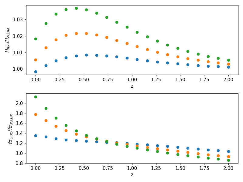
Figure 9: Comparison of the evolution of the ratio of observables in the Starobinsnky $f(R)$ models and their $\Lambda$CDM values. Each point is the theoretical prediction for a given redshift. Different colored curves correspond to different values of the model parameter, $\lambda^{-1}=0.3,0.7,1)$, with $\Omega_{m0}=0.3$ and $n=1$

One can build an $f(R)$ modified gravity model that mimics the background evolution of $\Lambda$CDM, like the one presented in section 2.1 and the well-known Hu-Sawicki model Hu2007 . Both models have a similar cosmological evolution, whereas the growth of structures is quite different to the $\Lambda$CDM model, owing to the scale dependence of the solution $\delta(k,a)$ of equation (19). In the refs. Linder2017 ; Matsumoto2020 it is shown how the $f\sigma_{8}-H$ plot can help distinguish between MG and $\Lambda$CDM-type models (i.e., $\Lambda$CDM or $w$CDM or $w_{0}w_{a}$CDM models with different parameters). To perform a similar analysis for our model, we fix the scale of our perturbations at $0.1h$/Mpc, around the scale where measurements and homogeneity assumptions in the $\Lambda$CDM model are made Avila21a ; Avila21b and a scale where linear perturbation theory is valid in $f(R)$ theories and nonlinear effects can be disregarded Koivisto2006 .

In figure 9, we see the separate plot of the ratio of $H(z)$ and $[f\sigma_{8}]/[f\sigma_{8\Lambda CDM}]$ for our Starobinsky $f(R)$ model and their $\Lambda$CDM values, respectively. For $H/H_{\Lambda CDM}$ the curves show similarity, also requiring a high amount of precision to distinguish the $<2\%$ absolute difference of the values, whereas for $[f\sigma_{8}](z)$ there is a high degeneracy in some redshift intervals between the same model with different parameters. This degeneracy makes it difficult to use data from this redshift interval to constrain the true $\lambda$ parameter of the model, while also, again, requiring a higher degree of precision to distinguish between the curves in this interval. For higher values of redshift, the degeneracy between the $f\sigma_{8}$ curves worsens, as they need to converge to the $\Lambda$CDM value by construction. Thus the redshift interval that allows us to constrain the true parameter of the model with good precision and low degeneracy between the curves is highly dependent on our ability to measure with high precision the local $H(z)$ history and the value of the model parameter. Using the $f\sigma_{8}/f\sigma_{8\Lambda CDM}\times H/H_{\Lambda CDM}$ joint analysis, devised by Matsumoto2020 and the similar $H(z)/H_{0}\times[f\sigma_{8}](z)$ from Linder2017 to plot the curves for our model, we see that the degeneracy between the different values of the parameters is manifestly broken considering the whole parameters space, as shown in figure 10.

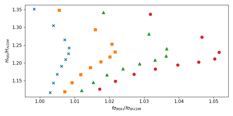
Figure 10: Curves on the $[f\sigma_{8}]/[f\sigma_{8}]_{\Lambda CDM}\times H/H_{\Lambda CDM}$ plane for different values of the $\lambda$ parameter, for the $n=1$ case. The curves, while having a similar profile, have different curvatures while also having different start and end points. From left to right we have $\lambda^{-1}=0.3,0.5,0.7,1$.

With the degeneracy broken, the only limiting factor in distinguishing the curves in the parameter space is the precision and the confidence interval of these measurements. Figure 11 shows how the parameter space can be further distinguished, including the $\Lambda$CDM model. While the expansion history of our (and general) $f(R)$ models follows the $\Lambda$CDM model closely enough that it can’t be distinguished from the standard model at the background level, when one conjoins just the $[f\sigma_{8}](z)$ evolution with the $H(z)$ expansion of the models, the degeneracy is clarified. Although there is still a degree of degeneracy between the curves, with the $H(z)/H_{0}$ data spanning a large interval, the difficulty in distinguishing between models lies, once again, in the precision of the available data.

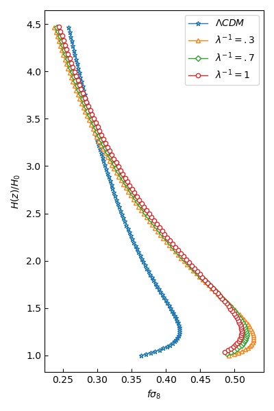
Figure 11: $[f\sigma_{8}](z)\times H(z)/H_{0}$ curves for the models $\Lambda$CDM and Starobinsky $f(R)$ with different values for the parameter $\lambda$ and $n=1$.

In Linder2017 the author gives an in depth analysis of the relevant redshift range to better distinguish dark energy models using this joint analysis of observables, also giving a preview of what future surveys will be able to give precise enough measurements to further break the degeneracy between models. An extensive analysis using similar methods with other MG models can be found in Matsumoto2020 . In Moresco2017 a similar analysis is done considering parameter extensions of the concordance $\Lambda$CDM model, with a likelihood approach. Here we’ll follow Moresco2017 in using the $f\sigma_{8}-H$ diagram to further distinguish between the parameters of our model.

4.2.1 Goodness of fit between models

We have produced a set of 5 binned data pairs, $(f\sigma_{8}(z)$, $H(z))$, for an equal number of redshift bins (see table 3); they were obtained by calculating the variance weighted mean in each redshift bin. We use this data to test goodness of fit procedure, via a $\chi^{2}$ methodology, to check which set of parameters best fits the joint data, obtained from the MCMC runs in 4.1. This analysis complements our likelihood analysis where we obtained best fit parameters from the three different sets of data described in 3. Here, we use the binned data to check which of the pair of parameters obtained from the exploration of parameter space best fits this joint data. Hereafter we’ll call each of the three different best fits obtained from the MCMC run a "model"; the model with the parameters given by the run on just the $H(z)$ data, the one from just $f\sigma_{8}(z)$ data and the one from the run on both datasets, referring to table 4.

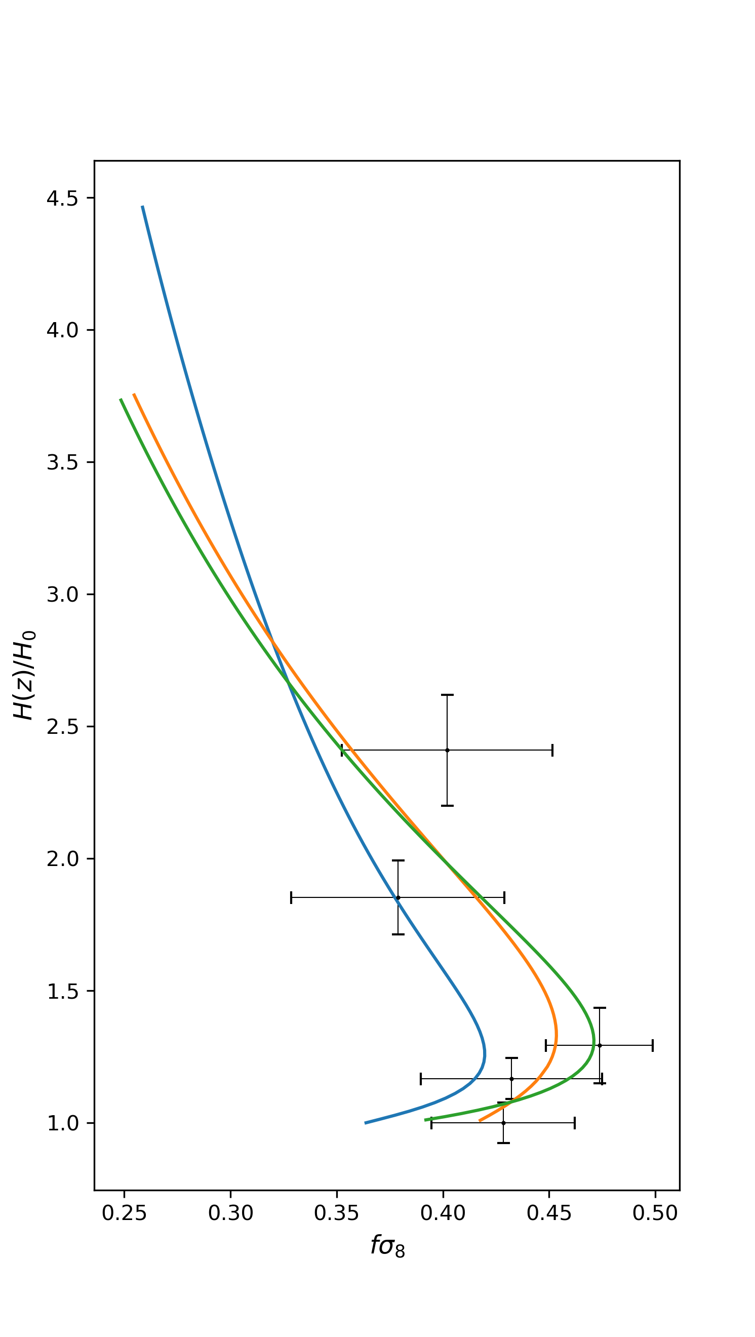
Figure 12: Goodness of fit test for binned data, from table 3. The blue curve corresponds to $\Lambda$CDM, the orange one to the Starobinsky $n=1$ model with the best-fit parameter $\lambda$, and the green one with the best-fit parameter for $n=2$, both found from the minimization of eq. (32) in the MCMC analyses.

We devised a simple 2D minimum squared weighted deviation (also a type of $\chi^{2}$), using the binned data from table 3. If, for each data point, we have the individual error on each variable, we have

• $\sigma_{f\sigma_{8}}\equiv$ $[f\sigma_{8}](z)$ error,

• $\sigma_{H}\equiv H(z)$ error,

and since the data for both observables are independent measurements, i.e., they are not correlated, we may write

$$\sigma^{2}\equiv\sigma^{2}_{\text{joint}}=\sigma^{2}_{H}+\sigma^{2}_{f\sigma 8},$$ (29)

as the joint error for both variables (termed variance in quadrature).

For each model we have a predicted value $(f\sigma_{8}(z_{i})$, $H(z_{i}))$ at redshift $z_{i}$, and a data point $(x_{i},y_{i})$ in the $f\sigma_{8}\times H(z)$ plane. The squared residual between the model prediction $P_{i}\equiv(f\sigma_{8}(z_{i}),H(z_{i}))$ and the observed data $O_{i}\equiv(x_{i},y_{i})$ is given by

$$(P_{i}-O_{i})^{2}=||(f\sigma_{8}(z_{i})-x_{i},H(z_{i})-y_{i})||^{2}\,,$$ (30)

where $||\cdot||$ is the distance between the two data points $(f\sigma_{8}(z_{i}),H(z_{i}))$ and $(x_{i},y_{i})$ in the $f\sigma_{8}\times H$ plane.

The $\chi^{2}$ is then defined as the sum of the square of the residuals averaged by the joint error for each data

$$\chi^{2}\equiv\sum^{n}_{i}\frac{(P_{i}-O_{i})^{2}}{\sigma_{i}^{2}}\,.$$ (31)

The reduced mean squared weighted deviation is then, for each model analyzed, the ratio between $\chi^{2}$ and the number of degrees of freedom $\nu$, $\nu=n-m=5-2=3$ for the Starobinsky models, and $\nu=5-1=4$ for the flat $\Lambda CDM$ model

$$\chi^{2}_{\nu}=\frac{\chi^{2}}{\nu}\,.$$ (32)

In our case the flat $\Lambda$CDM model has one free parameter $\Omega_{\Lambda 0}$ (where $\Omega_{m0}$ is constrained by the algebraic relation $\Omega_{\Lambda 0}+\Omega_{m0}=1$ ), one less than the Starobinsky models analysed, i.e., $\Omega_{m0}$ and $\lambda^{-1}$.

Each MCMC parameter space exploration results in a best fit of the model via the likelihood minimization performed by the MCMC method. We performed three sets of MCMC runs for each of the cases $n=1$ and $n=2$, each on a different data set, described in section 3; here we treat each result as a different model, and test the models against the binned data (see table 3).

Model	$\Omega_{m0}$	$\lambda^{-1}$	$\chi_{\nu}^{2}$
Starobinsky $n=1$, $\lambda$ best-fit with $H(z)$	0.335	1.76	6.26
Starobinsky $n=1$, $\lambda$ best-fit with $[f\sigma_{8}](z)$	0.204	1.46	0.99
Starobinsky $n=1$, $\lambda$ best-fit with joint data	0.337	1.19	5.014
Starobinsky $n=2$, $\lambda$ best-fit with $H(z)$	0.351	0.38	3.63
Starobinsky $n=2$, $\lambda$ best-fit with $[f\sigma_{8}](z)$	0.185	1.8	1.61
Starobinsky $n=2$, $\lambda$ best-fit with joint data	0.205	0.99	1.02
$\Lambda$CDM	0.28	–	0.69

Table 5: Goodness of fit test, measured by $\chi_{\nu}^{2}$ through the analysis of the binned data in table 3, to compare the behavior of the $\Lambda$CDM and 3 Starobinsky models (each with a best-fitted $\lambda$ parameter provided by the MCMC runs considering 3 data sets).

We then calculate (32) for each of our models and the minimization of this parameter gives a naive estimate of the model that best fits the data in the $f\sigma_{8}\times H$ plane. The results of this naive analysis allow us to differentiate between models with different values of $\lambda$ obtained from the MCMC run, which can be seen in table 5. The model that best fits the data according to this criterium is plotted in figure 12

From the $\chi^{2}$ statistics, we see that the $\Lambda$CDM model is, from this joint data set, the one with the smallest $\chi^{2}_{\nu}$ value, naively giving an "overfit" to the data; with the $n=2$ case having the best fit with all data sets, in comparison with the $n=1$ case. This is expected, as per the observational problems mentioned before concerning the $n=1$ model, and from the fact that the parameter $n=1$ is in direct relation to deviations from $\Lambda$CDM; $n=1$ being the integer value greater than $0$ that deviates the most from the concordance model. As for the "overfit" of the $\Lambda$CDM model, it’s also important to note that the model has 1 parameter less than the $f(R)$ models, which gives it a lower value from the reduced $\chi^{2}$ statistics.

While one could say that $\Lambda$CDM fits the joint data better than any version of the Starobinsky models from the $\chi^{2}$ test, some observations on the methods and data are in order. First, it’s interesting to note that the $f\sigma_{8}$ data alone gives a better fit to the joint data than the result from the MCMC run on data from both $[f\sigma_{8}](z)$ and $H(z)$ data, in the $n=1$ case. This could be the case for diverse reasons; one being that the $H(z)$ is actually worsening the results from the $[f\sigma_{8}](z)$ data when analyzed together. As expected theoretically, background quantities don’t constrain modified gravity models suitably; the MCMC run on the $H(z)$ data alone, found in 3, was not able to constraint the free parameters analyzing the $[f\sigma_{8}](z)$ data. In the $n=2$ case, the joint data constrains the $\lambda$ parameter significantly better than both the $H$ and $f\sigma_{8}$ alone, while also giving a better fit from the $\chi^{2}$ test in general, as can be seen from figure 12. This points to a fault with the $n=1$ model once again.

Also, the binned data presented in table 3, built from the $H(z)$ and $[f\sigma_{8}](z)$ datasets, gives us 5 data points for goodness of fit analysis. As a test on whether the binning choice affects the $\chi^{2}$ statistics, we considered other binned sets and found similar results. The advantage of this approach is that it allows to break of the degeneracy between models with dissimilar $\lambda$ parameter, but due to the large errors at high$-z$ the analysis is not as accurate as desirable to clearly discriminate between the $\Lambda$CDM and the Starobinsky models. This could also explain the "overfitting" of the $\Lambda$CDM model, which would give a $\chi^{2}$ closer to 1 if the error was better constrained. In fact, more data points and tighter error constraints are needed to improve the significance of the goodness of fit. This means not only precise measurements on these observables, in particular at high$-z$, but also data in more redshift intervals. From our MCMC analysis, we observe that the data on $[f\sigma_{8}](z)$ was able to better constraint the parameters of the $f(R)$ model in both cases, thus results from upcoming surveys such as the DESI, SKA, and EUCLID telescopes Maartens_2020 will be able to probe the growth of cosmic structures with precision to greatly improve the significance of this kind of analysis.

It is important to note that the conjoined analysis found in table 5, even if with low statistical significance, was able to differentiate between different models inside the same $f(R)$ theory, and in particular with the same $n$ parameter, which we saw had high degeneracy in the $H(z)$ observables, and some degeneracy in $[f\sigma_{8}](z)$. Thus the proposal of Linder2017 ; Matsumoto2020 of breaking this degeneracy between models using the conjoined data is effectual.

4.3 Remarks on stability and solar system test

From the results of the MCMC runs, seen in 4, and from the constraints on the theory in (11), that give $\lambda^{-1}<0.21$ for the $n=1$ case, and $\lambda^{-1}<1.578$ for $n=2$, we see that no best fit for $\lambda$ in the $n=1$ case gives a stable model of the theory, while in the $n=2$ case the best fit with the $f\sigma_{8}$ dataset gives a fit that does not pass the de Sitter stability criteria. This once again shows some of the issues with the $n=1$ model.

As for the solar system test, the constraint comes mainly from the PPN parameter $\gamma$, which, from the Cassini probe, has to satisfy the constraint Negrelli_2020 ; Starobinsky2007

$$|\gamma-1|<4\times 10^{-4}.$$ (33)

In a recent paper on solar system tests on $f(R)$ theories, Negrelli_2020 has shown that a model with the parameters $\lambda=\lambda^{-1}=1$, $R_{0}=4.17H_{0}^{2}$ and $n=2$ easily passes the (33) constraint and the chameleon tests in the solar system. From the best fit parameters obtained in 5, we see that the best fit parameters for the $n=2$ are well inside the constraint obtained in Negrelli_2020 , since $R_{0}\lambda=6\lambda(1-\Omega_{m0})H_{0}^{2}<4H_{0}^{2}$ for all the cases.

For the $n=1$ case, it is known since the original Starobinsky’s work Starobinsky2007 that for $n=1$ the model does not satisfy the constraints from the solar system test.

5 Conclusions and Final Remarks

In this paper, we have used the cosmic expansion and the structure growth data to constrain the free parameters of a relevant $f(R)$ gravity model, namely the Starobinsky model. We’ve used the bayesian based Monte Carlo Markov Chain method to explore the parameter space of this model from both sets of data individually and using a joint likelihood analysis. Furthermore, we also used the recent method proposed by Linder Linder2017 and Matsumoto et al. Matsumoto2020 to complement the result of the MCMC statistical analysis. This novel approach, based on a joint data analyses from $H$ and $f\sigma_{8}$, has proven able to give further distinction between different models which were shown to have degeneracy in the theoretical predictions of the $H(z)$ and $[f\sigma_{8}](z)$ observables in the range of the free parameters of the $f(R)$ model.

In the end, our results show that in the $f(R)$ Starobinsky model, for $n=1$ the model is not very well constrained but the data from $f\sigma_{8}$ gives a good fit to the joint data, where for $n=2$, the parameters are significantly better constrained and the joint data gives a great fit. The $\Lambda$CDM has the smallest $\chi^{2}$ value for the test, as expected. This joint analysis gives another observational result in motivating $n\geq 2$ in the $f(R)$ Starobinsky model. However more –and more precise– data are needed in order to determine the preferred model with good statistical significance. The joint binned data set still gives space to overfitting from the $\Lambda$CDM model and big error margins in the parameter space of the $f(R)$ models. Therefore, the Starobinsky model cannot be discarded as a possible alternative to the $\Lambda$CDM model, still passing all the observational tests for $n\geq 2$.

A possible continuation of this work would be to use this joint analysis to compare diverse cosmologically motivated $f(R)$ models, such as the one in Hu2007 and the one in this paper break the degeneracy between different $f(R)$ theories. The results of this paper show that this method is promising for further distinction between modified gravity models that are degenerate in certain cosmological probes. The extension of this analysis is left for future work.

References

- [1] A. A. Starobinsky. Disappearing cosmological constant in f(r) gravity. JETP Letters, 86(3):157–163, Oct 2007.
- [2] Eric V. Linder. Cosmic growth and expansion conjoined. Astroparticle Physics, 86:41–45, 2017.
- [3] P. A. R. Ade et al. Planck 2015 results. XIV. Dark energy and modified gravity. Astron. Astrophys., 594:A14, 2016.
- [4] N. Aghanim et al. Planck 2018 results. VI. Cosmological parameters. Astron. Astrophys., 641:A6, 2020. [Erratum: Astron.Astrophys. 652, C4 (2021)].
- [5] Lavrentios Kazantzidis and Leandros Perivolaropoulos. Evolution of the tension with the Planck15/CDM determination and implications for modified gravity theories. Phys. Rev. D, 97(10):103503, 2018.
- [6] Spyros Basilakos and Fotios K. Anagnostopoulos. Growth index of matter perturbations in the light of dark energy survey. The European Physical Journal C, 80(3), Mar 2020.
- [7] Eric V. Linder. Limited modified gravity. Journal of Cosmology and Astroparticle Physics, 2020(10):042–042, Oct 2020.
- [8] A. M. Velasquez-Toribio and Júlio C. Fabris. The growth factor parametrization versus numerical solutions in flat and non-flat dark energy models. The European Physical Journal C, 80(12), Dec 2020.
- [9] Alexander Bonilla, Suresh Kumar, and Rafael C. Nunes. Measurements of and reconstruction of the dark energy properties from a model-independent joint analysis. The European Physical Journal C, 81(2), Feb 2021.
- [10] Zahra Davari and Sohrab Rahvar. Mog cosmology without dark matter and the cosmological constant. Monthly Notices of the Royal Astronomical Society, 507(3):3387–3399, Aug 2021.
- [11] Eric V. Linder and Robert N. Cahn. Parameterized beyond-einstein growth. Astroparticle Physics, 28(4):481 – 488, 2007.
- [12] H. B. Benaoum, Weiqiang Yang, Supriya Pan, and Eleonora Di Valentino. Modified Emergent Dark Energy and its Astronomical Constraints. arXiv e-prints, page arXiv:2008.09098, August 2020.
- [13] Louis Perenon, Federico Piazza, Christian Marinoni, and Lam Hui. Phenomenology of dark energy: general features of large-scale perturbations. JCAP, 11:029, 2015.
- [14] Louis Perenon, Julien Bel, Roy Maartens, and Alvaro de la Cruz-Dombriz. Optimising growth of structure constraints on modified gravity. JCAP, 2019(6):020, June 2019.
- [15] Louis Perenon, Stéphane Ilíc, Roy Maartens, and Alvaro de la Cruz-Dombriz. Improvements in cosmological constraints from breaking growth degeneracy. Astron. Astrophys., 642:A116, 2020.
- [16] Ronaldo C. Batista. Impact of dark energy perturbations on the growth index. Phys. Rev. D, 89(12):123508, 2014.
- [17] Rafael C. Nunes. Structure formation in gravity and a solution for tension. JCAP, 05:052, 2018.
- [18] David Benisty and Eduardo I. Guendelman. Unified dark energy and dark matter from dynamical spacetime. Phys. Rev. D, 98(2):023506, 2018.
- [19] Fotios K. Anagnostopoulos, David Benisty, Spyros Basilakos, and Eduardo I. Guendelman. Dark energy and dark matter unification from dynamical space time: observational constraints and cosmological implications. JCAP, 06:003, 2019.
- [20] David Benisty, Eduardo Guendelman, and Zbigniew Haba. Unification of dark energy and dark matter from diffusive cosmology. Phys. Rev. D, 99(12):123521, 2019. [Erratum: Phys.Rev.D 101, 049901 (2020)].
- [21] Wayne Hu and Ignacy Sawicki. Models of f(R) Cosmic Acceleration that Evade Solar-System Tests. Physical Review D, may 2007.
- [22] Timothy Clifton, Pedro G. Ferreira, Antonio Padilla, and Constantinos Skordis. Modified Gravity and Cosmology. Physics Reports, jun 2011.
- [23] Matteo Martinelli, Erminia Calabrese, Francesco De Bernardis, Alessandro Melchiorri, Luca Pagano, and Roberto Scaramella. Constraining modified gravitational theories by weak lensing with euclid. Physical Review D, 83(2), Jan 2011.
- [24] Michael A. Strauss and Jeffrey A. Willick. The density and peculiar velocity fields of nearby galaxies. Physics Reports, 261(5):271 – 431, 1995.
- [25] Spyros Basilakos. The cdm growth rate of structure revisited. International Journal of Modern Physics D, 21(07):1250064, 2012.
- [26] Jiro Matsumoto, Teppei Okumura, and Misao Sasaki. New measures to test modified gravity cosmologies. Journal of Cosmology and Astroparticle Physics, 2020(7), jul 2020.
- [27] Antonio de Felice and Shinji Tsujikawa. f (R) theories. Living Reviews in Relativity, 13, 2010.
- [28] Yow-Chun Chen, Chao-Qiang Geng, Chung-Chi Lee, and Hongwei Yu. Matter Power Spectra in Viable Gravity Models with Dynamical Background. The European Physical Journal C, 79(2):93, jan 2019.
- [29] Michael Kopp, Stephen A. Appleby, Ixandra Achitouv, and Jochen Weller. Spherical collapse and halo mass function inf(r)theories. Physical Review D, 88(8), oct 2013.
- [30] Hayato Motohashi, Alexei A. Starobinsky, and Junichi Yokoyama. Analytic solution for matter density perturbations in a class of viable cosmological f(r) models. International Journal of Modern Physics D, 18(11):1731–1740, nov 2009.
- [31] Vincenzo F Cardone, Stefano Camera, and Antonaldo Diaferio. An updated analysis of two classes of f(r) theories of gravity. Journal of Cosmology and Astroparticle Physics, 2012(02):030–030, Feb 2012.
- [32] Renier Hough, Amare Abebe, and Stefan Ferreira. Viability tests of f(R)-gravity models with Supernovae Type 1A data, 2020.
- [33] Hayato Motohashi, Alexei A. Starobinsky, and Jun’ichi Yokoyama. Cosmology based on f(r) gravity admits 1 ev sterile neutrinos. Physical Review Letters, 110(12), mar 2013.
- [34] Anton S. Chudaykin, Dmitry S. Gorbunov, Alexei A. Starobinsky, and Rodion A. Burenin. Cosmology based on f(r) gravity with (1) eV sterile neutrino. Journal of Cosmology and Astroparticle Physics, 2015(05):004–004, 2015.
- [35] Thomas P. Sotiriou and Valerio Faraoni. f(r)theories of gravity. Reviews of Modern Physics, 82(1):451–497, Mar 2010.
- [36] Hayato Motohashi, Alexei A Starobinsky, and Junichi Yokoyama. Future oscillations around phantom divide inf(r) gravity. Journal of Cosmology and Astroparticle Physics, 2011(06):006–006, jun 2011.
- [37] Shinji Tsujikawa. Matter density perturbations and effective gravitational constant in modified gravity models of dark energy. Physical Review D, 76(2), Jul 2007.
- [38] Raul Jimenez and Abraham Loeb. Constraining cosmological parameters based on relative galaxy ages. The Astrophysical Journal, 573(1):37–42, jul 2002.
- [39] Yingjie Yang and Yungui Gong. The evidence of cosmic acceleration and observational constraints. Journal of Cosmology and Astroparticle Physics, 2020(06):059–059, jun 2020.
- [40] Nick Kaiser. Clustering in real space and in redshift space. MNRAS, 227:1–21, July 1987.
- [41] A. J. S. Hamilton. Measuring Omega and the Real Correlation Function from the Redshift Correlation Function. APJL, 385:L5, January 1992.
- [42] F. Avila, C. P. Novaes, A. Bernui, E. de Carvalho, and J. P. Nogueira-Cavalcante. The angular scale of homogeneity in the Local Universe with the SDSS blue galaxies. Mon. Not. Roy. Astron. Soc., 488(1):1481–1487, 2019.
- [43] Gabriela A. Marques and Armando Bernui. Tomographic analyses of the CMB lensing and galaxy clustering to probe the linear structure growth. JCAP, 05:052, 2020.
- [44] E. de Carvalho, A. Bernui, G. C. Carvalho, C. P. Novaes, and H. S. Xavier. Angular Baryon Acoustic Oscillation measure at from the SDSS quasar survey. JCAP, 04:064, 2018.
- [45] E. de Carvalho, A. Bernui, H. S. Xavier, and C. P. Novaes. Baryon acoustic oscillations signature in the three-point angular correlation function from the SDSS-DR12 quasar survey. Mon. Not. Roy. Astron. Soc., 492(3):4469–4476, 2020.
- [46] Rafael C. Nunes, Edésio M. Barboza, Jr., Everton M. C. Abreu, and Jorge Ananias Neto. Probing the cosmological viability of non-gaussian statistics. JCAP, 08:051, 2016.
- [47] Shadab Alam, Marie Aubert, Santiago Avila, Christophe Balland, Julian E. Bautista, Matthew A. Bershady, Dmitry Bizyaev, Michael R. Blanton, Adam S. Bolton, Jo Bovy, and et al. Completed sdss-iv extended baryon oscillation spectroscopic survey: Cosmological implications from two decades of spectroscopic surveys at the apache point observatory. Physical Review D, 103(8), Apr 2021.
- [48] F. Avila, A. Bernui, E. de Carvalho, and C. P. Novaes. The growth rate of cosmic structures in the local Universe with the ALFALFA survey. Mon. Not. Roy. Astron. Soc., 505(3):3404–3413, 2021.
- [49] Stephen J. Turnbull, Michael J. Hudson, Hume A. Feldman, Malcolm Hicken, Robert P. Kirshner, and Richard Watkins. Cosmic flows in the nearby universe from type ia supernovae. Monthly Notices of the Royal Astronomical Society, 420(1):447–454, Dec 2011.
- [50] Dragan Huterer, Daniel L. Shafer, Daniel M. Scolnic, and Fabian Schmidt. Testing cdm at the lowest redshifts with sn ia and galaxy velocities. Journal of Cosmology and Astroparticle Physics, 2017(05):015–015, May 2017.
- [51] I. Achitouv, C. Blake, P. Carter, J. Koda, and F. Beutler. Consistency of the growth rate in different environments with the 6-degree field galaxy survey: Measurement of the void-galaxy and galaxy-galaxy correlation functions. Physical Review D, 95(8), Apr 2017.
- [52] Florian Beutler, Chris Blake, Matthew Colless, D. Heath Jones, Lister Staveley-Smith, Gregory B. Poole, Lachlan Campbell, Quentin Parker, Will Saunders, and Fred Watson. The 6df galaxy survey: measurements of the growth rate and . Monthly Notices of the Royal Astronomical Society, 423(4):3430–3444, Jun 2012.
- [53] Martin Feix, Adi Nusser, and Enzo Branchini. Growth rate of cosmological perturbations at from a new observational test. Physical Review Letters, 115(1), Jun 2015.
- [54] Ariel G. Sánchez, Francesco Montesano, Eyal A. Kazin, Eric Aubourg, Florian Beutler, Jon Brinkmann, Joel R. Brownstein, Antonio J. Cuesta, Kyle S. Dawson, Daniel J. Eisenstein, and et al. The clustering of galaxies in the sdss-iii baryon oscillation spectroscopic survey: cosmological implications of the full shape of the clustering wedges in the data release 10 and 11 galaxy samples. Monthly Notices of the Royal Astronomical Society, 440(3):2692–2713, Apr 2014.
- [55] Chris Blake, Sarah Brough, Matthew Colless, Carlos Contreras, Warrick Couch, Scott Croom, Darren Croton, Tamara M. Davis, Michael J. Drinkwater, Karl Forster, and et al. The wigglez dark energy survey: joint measurements of the expansion and growth history atz< 1. Monthly Notices of the Royal Astronomical Society, 425(1):405–414, Jul 2012.
- [56] Seshadri Nadathur, Paul M. Carter, Will J. Percival, Hans A. Winther, and Julian E. Bautista. Beyond bao: Improving cosmological constraints from boss data with measurement of the void-galaxy cross-correlation. Physical Review D, 100(2), Jul 2019.
- [57] Chia-Hsun Chuang, Francisco Prada, Marcos Pellejero-Ibanez, Florian Beutler, Antonio J. Cuesta, Daniel J. Eisenstein, Stephanie Escoffier, Shirley Ho, Francisco-Shu Kitaura, Jean-Paul Kneib, and et al. The clustering of galaxies in the sdss-iii baryon oscillation spectroscopic survey: single-probe measurements from cmass anisotropic galaxy clustering. Monthly Notices of the Royal Astronomical Society, 461(4):3781–3793, Jun 2016.
- [58] A. Pezzotta, S. de la Torre, J. Bel, B. R. Granett, L. Guzzo, J. A. Peacock, B. Garilli, M. Scodeggio, M. Bolzonella, U. Abbas, and et al. The vimos public extragalactic redshift survey (vipers). Astronomy & Astrophysics, 604:A33, Jul 2017.
- [59] Marie Aubert, Marie-Claude Cousinou, Stéphanie Escoffier, Adam J. Hawken, Seshadri Nadathur, Shadab Alam, Julian Bautista, Etienne Burtin, Arnaud de Mattia, Héctor Gil-Marín, Jiamin Hou, Eric Jullo, Richard Neveux, Graziano Rossi, Alex Smith, Amélie Tamone, and Mariana Vargas Magaña. The completed sdss-iv extended baryon oscillation spectroscopic survey: Growth rate of structure measurement from cosmic voids, 2020.
- [60] Michael J. Wilson. Geometric and growth rate tests of general relativity with recovered linear cosmological perturbations, 2016.
- [61] Gong-Bo Zhao, Yuting Wang, Shun Saito, Héctor Gil-Marín, Will J Percival, Dandan Wang, Chia-Hsun Chuang, Rossana Ruggeri, Eva-Maria Mueller, Fangzhou Zhu, and et al. The clustering of the sdss-iv extended baryon oscillation spectroscopic survey dr14 quasar sample: a tomographic measurement of cosmic structure growth and expansion rate based on optimal redshift weights. Monthly Notices of the Royal Astronomical Society, 482(3):3497–3513, Oct 2018.
- [62] Teppei Okumura, Chiaki Hikage, Tomonori Totani, Motonari Tonegawa, Hiroyuki Okada, Karl Glazebrook, Chris Blake, Pedro G. Ferreira, Surhud More, Atsushi Taruya, and et al. The subaru fmos galaxy redshift survey (fastsound). iv. new constraint on gravity theory from redshift space distortions at . Publications of the Astronomical Society of Japan, 68(3):38, Apr 2016.
- [63] M. Moresco and F. Marulli. Cosmological constraints from a joint analysis of cosmic growth and expansion. Monthly Notices of the Royal Astronomical Society: Letters, 471(1):L82–L86, 2017.
- [64] Adam G. Riess, Stefano Casertano, Wenlong Yuan, Lucas M. Macri, and Dan Scolnic. Large Magellanic Cloud Cepheid Standards Provide a 1% Foundation for the Determination of the Hubble Constant and Stronger Evidence for Physics beyond CDM. Astrophys. J., 876(1):85, 2019.
- [65] Rafael C. Nunes and Armando Bernui. BAO signatures in the 2-point angular correlations and the Hubble tension. Eur. Phys. J. C, 80(11):1025, 2020.
- [66] Fotios K. Anagnostopoulos and Spyros Basilakos. Constraining the dark energy models with h(z) data: An approach independent of h0. Physical Review D, 97(6), Mar 2018.
- [67] Daniel Foreman-Mackey, David W. Hogg, Dustin Lang, and Jonathan Goodman. emcee: The mcmc hammer. Publications of the Astronomical Society of the Pacific, 125(925):306–312, Mar 2013.
- [68] Gabriela A. Marques, Jia Liu, José Manuel Zorrilla Matilla, Zoltán Haiman, Armando Bernui, and Camila P. Novaes. Constraining neutrino mass with weak lensing Minkowski Functionals. JCAP, 06:019, 2019.
- [69] P. A. R. Ade, N. Aghanim, M. Arnaud, M. Ashdown, J. Aumont, C. Baccigalupi, A. J. Banday, R. B. Barreiro, J. G. Bartlett, and et al. Planck2015 results. Astronomy & Astrophysics, 594:A13, Sep 2016.
- [70] F. Avila, A. Bernui, R. C. Nunes, E. de Carvalho, and C. P. Novaes. The homogeneity scale and the growth rate of cosmic structures. Monthly Notices of the Royal Astronomical Society, 2021.
- [71] Tomi Koivisto. Matter power spectrum in f(R) gravity. Physical Review D - Particles, Fields, Gravitation and Cosmology, 73(8):1–5, 2006.
- [72] Jan-Albert Viljoen, José Fonseca, and Roy Maartens. Constraining the growth rate by combining multiple future surveys. Journal of Cosmology and Astroparticle Physics, 2020(09):054–054, Sep 2020.
- [73] Carolina Negrelli, Lucila Kraiselburd, Susana J. Landau, and Marcelo Salgado. Solar system tests and chameleon effect in f(r) gravity. Physical Review D, 101(6), mar 2020.