ReIGNN: State Register Identification Using Graph Neural Networks for Circuit Reverse Engineering

Abstract

Reverse engineering an integrated circuit netlist is a powerful tool to help detect malicious logic and counteract design piracy. A critical challenge in this domain is the correct classification of data-path and control-logic registers in a design. We present ReIGNN, a novel learning-based register classification methodology that combines graph neural networks (GNNs) with structural analysis to classify the registers in a circuit with high accuracy and generalize well across different designs. GNNs are particularly effective in processing circuit netlists in terms of graphs and leveraging properties of the nodes and their neighborhoods to learn to efficiently discriminate between different types of nodes. Structural analysis can further rectify any registers misclassified as state registers by the GNN by analyzing strongly connected components in the netlist graph. Numerical results on a set of benchmarks show that ReIGNN can achieve, on average, 96.5% balanced accuracy and 97.7% sensitivity across different designs.

I Introduction

Integrated circuits (ICs) are often considered the root of trust of modern computing systems. However, the globalization of the IC supply chain[1] and the reliance on third-party resources, including third-party intellectual property (IP) cores and fabrication foundries, have brought into question IC protection against threats like IP piracy, counterfeiting [2, 3], and hardware Trojan (HT) insertion [4]. Reverse engineering is a promising tool to restore trust in the IC supply chain by enabling the identification of malicious modifications in a design.

Hardware reverse engineering consists in extracting the high-level functionality of a design through multiple automated or manual analysis steps. The first step is to obtain the gate-level netlist from a fabricated chip through delayering, imaging, and post processing [5, 2, 6]. Once the netlist is available, gate-level netlist reverse engineering techniques are employed to infer the functionality of the netlist. Netlist reverse engineering consists of two main tasks, namely, data-path reverse engineering and control-logic reverse engineering. The control logic in a digital circuit is in charge of generating signals to control the data path. Data-path blocks are more suitable for algorithmic analysis, due to their regularity and high degree of replication, using techniques like template matching [7], behavioral matching of an unknown sub-circuit against a library of abstract components [8] or machine learning (ML)-based circuit recognition [9]. On the other hand, the control logic of a design is generally designed for a specific functionality, which makes it difficult to apply the techniques mentioned above. Reverse engineering the control logic involves the identification of the state registers followed by a finite state machine (FSM) extraction step, which recovers the state transition graph (STG) [10, 11, 12, 13] of the circuit FSM. Correct identification of the state registers is, therefore, instrumental in the extraction of a correct FSM.

Many techniques have been proposed to identify the state registers [14, 15, 16] in a design. Techniques like RELIC [14] and fastRELIC [15] are based on the detection of similarities between the topologies of the registers’ fan-in circuits. However, they tend to depend on fine-tuning of a set of configuration parameters for each circuit to achieve high accuracy. When little or no information is available about a design netlist, it becomes challenging to converge on the parameter values which can lead to the best result. Moreover, the complexity of these techniques varies polynomially with the number of registers in a design, i.e., the higher the number of registers, the higher the classification time.

Inspired by the success of state-of-the-art deep learning (DL) methods in solving different challenging problems across different fields, we present ReIGNN (Register Identification Using Graph Neural Networks), a novel learning-based technique to classify the state and data registers in a netlist. ReIGNN combines GNNs with structural analysis to achieve high accuracy and generalization properties across different designs. GNNs are deep learning models that operate directly on graphs and adeptly perform different graph-related learning and inference tasks like node classification by leveraging the graph structure, the properties of the nodes, and the characteristics of their neighborhoods. By mapping the circuit gates and registers to graph nodes and their connections to graph edges, the register classification task directly translates into a node classification problem. In ReIGNN, we automatically abstract the circuit netlist as a graph and associate each graph node with a feature vector that captures information about its functionality and connectivity. We then train the GNN that processes these graphs to discriminate between state and data registers in the netlist. The trained GNNs can then be used to classify the registers of new netlists. Finally, we perform structural analysis of the netlist and, specifically, identification of strongly connected components that include registers in the graph, to further improve the accuracy of the GNN and rectify misclassifications. In summary, this paper makes the following contributions:

• The identification and efficient extraction of a set of features for each gate and register in a netlist to capture their functionality as well as connectivity properties.

• ReIGNN, a novel learning-based methodology which combines GNNs with structural analysis to classify the registers in a circuit. To the best of our knowledge, this is the first GNN-based circuit register classification method.

Empirical results on a dataset containing standard circuit designs show that ReIGNN can achieve, on average, 96.5% balanced accuracy and 97.7% sensitivity across the different designs.

The remainder of this paper is structured as follows. In Section II we discuss the related work. Section III provides background notions at the basis of our technique. We describe the learning-based register classification methodology in Section IV and its detailed evaluation in Section V. Finally, we conclude in Section VI.

II Related Work

Reverse engineering the control logic of a circuit aims at extracting an FSM from the gate-level netlist [15]. The first and often most critical step in FSM extraction is the correct classification of the state and data registers. Many techniques have been proposed over the years to perform this task. A register can be classified as a state register if it has a feedback path [11], based on the observation that the state registers in an FSM always have a logic path from their output to the input, as shown in Fig. 1. However, the accuracy of a technique exclusively based on this rule tends to be poor since it neglects that many data-path designs employ data registers including feedback paths. Shi et al. [10] improve the classification accuracy by eliminating all the candidate state registers that do not affect a control signal like the select line of a multiplexer or the enable input of a register. More recently, the reset signal, control behavior, and feedback path information associated with the registers have been used together with strongly connected component (SCC) analysis to improve on the results of previous methods [13]. While ReIGNN leverages graph algorithms and SCC, it differs from previous techniques in that it also uses the structural and functional properties of each element of the netlist.

Another category of reverse engineering techniques compare the registers’ fan-in circuits either topologically or functionally to determine the type of registers, by exploiting the replication of circuit structures occurring naturally in the implementation of multi-bit data-path designs. RELIC [14] performs a similarity test between all pairs of registers’ fan-in circuits to identify potential state registers. Given two registers, it computes a “similarity” score between $0$ and $1$. Intuitively, data-path registers may be clustered into groups that implement the same functionality, hence they have similar fan-in circuit structure. On the other hand, state registers do not generally have similar fan-in circuit structures because the FSM state transitions tend to depend on unique logic conditions. Different state registers tend to relate to different transition logic blocks. The registers are then classified based on pre-defined threshold values and the similarity scores. fastRELIC [15] improves the performance of RELIC by reducing the number of register pair comparisons and by considering not only the similarity between the registers’ original fan-in circuits, but also the similarity between the original and the inverse fan-in circuits, obtained by replacing the AND and OR gates with OR and AND gates, respectively, and inverting the inputs [17] of the original fan-in circuits. A greedy register clustering algorithm is used to group the registers based on the similarity of the structure of their fan-in circuits. Instead of comparing each register with every other register in the design, the comparison is performed with only one member of a cluster. However, the choice of the member is based on heuristics, and the worst-case complexity is the same as RELIC.

Figure 1: Block diagram of an FSM. In a Moore machine, the output function logic depends on the current state only. In a Mealy machine, the output is a function of both the current state and the input (dotted line).

Subramanyan et al. [18, 19] compare the registers’ fan-in logic functions rather than their structure. Cut-based Boolean function matching is used to find replicated bit-slices in the netlist so that all the data registers can be identified and aggregated into words. A bit-slice is a Boolean function with one output and a small number of inputs. RELIC-FUN [16] uses the same algorithmic approach but focuses on finding registers whose fan-in logic implements different functions. Unlike these techniques [14, 15, 16], ReIGNN does not require pairwise comparisons of the structure or function of the registers’ fan-in circuits or pre-calibration of threshold values for similarity scores, since the registers of an unknown circuit are directly classified by the trained GNN.

DL has been recently used for different tasks in the context of hardware security, e.g., to detect HTs [4, 20, 21], attack logic locking [22, 23, 24, 25], or identify the functionality of data-path building blocks [9, 6]. GNNs have also been used for attacking logic locking [26]. Our work is different, since it uses DL models, and specifically GNNs, for classifying the registers in a netlist, which is the first step toward reverse engineering the circuit control logic.

III Preliminaries

This section outlines some background concepts that will be used throughout the paper.

III-A FSM Model

We model the control logic of a circuit as an FSM, a computational model characterized by a finite number of states. Depending on the input and the current state, the FSM transitions to the next state at each reaction and generates output control signals [13].

Definition 1 (FSM).

An FSM is a 6-tuple $(S,I,s_{0},\delta,O,\omega)$ where $S$ is the finite set of states, $I$ is the finite set of inputs, $O$ is the finite set of outputs, $s_{0}\in S$ is the initial state, $\delta:S\times I\rightarrow S$ is the state transition function which determines the next state depending on the input and the current state, and $\omega$ is the output function logic.

Figure 1 shows the block diagram representation of an FSM which consists of: (a) the next state logic computing $\delta$, (b) a state register that stores the current state $S$, and (c) the output function logic that computes $\omega$. All the state registers in an FSM are connected to the same $clock$ signal, which is used to trigger the FSM reaction. The states can be encoded using different styles to meet different design goals. For example, when using one-hot encoding, $|S|$-bit registers are required to represent the state, $|S|$ being the cardinality of the set $S$. The number of required registers is higher than with binary encoding, which only uses $\lceil\log_{2}|S|\rceil$-bit registers [27]. In this paper, we denote a memory element that stores one bit of the encoded state of an FSM as state register. All other memory elements in the design are denoted as data registers.

III-B RELIC

We detail RELIC [14], which will be used as a reference method to compare with ReIGNN. RELIC pre-processes a gate-level netlist such that it contains only AND, OR, and INV gates, to ensure that similar logic functions are represented by similar circuit structures [14]. A topological similarity test is then performed on the pre-processed netlists to calculate the similarity score between every register pair, as denoted by the SimilarityScore function in Algorithm 1. The calculated similarity score lies between $0$ (no similarity) and $1$ (identical fan-in circuit structure). RELIC first creates a bipartite graph with the fan-in nodes of the registers. The fan-in nodes are then compared recursively and, if their similarity score is above $T1$, an edge is connected to the bipartite graph. To avoid a large number of recursive calls to the SimilarityScore function, the analysis of the fan-in circuits is limited to a maximum depth d. A maximum matching algorithm is then executed on the bipartite graph to generate the similarity score between two registers. If this similarity score is above $T2$, then the similarity count of both registers is incremented by one. Finally if the similarity count of a register is above $T3$, then it is classified as a data register. RELIC requires the user to define these three threshold parameters, $T1,T2$, and $T3$, together with the depth of the fan-in circuits.

Algorithm 1 RELIC

1:

2:$graph$: the graph generated from the netlist

3:$registers$: the list of registers in the netlist

4:$T1,T2,T3$: three threshold values selected by the user to tune the result of RELIC

5:$d$: depth of the registers’ fan-in logic circuits

6:

7:function SimilarityScore($i,j,d,T1$)

8:    $max\_children\leftarrow\textsc{max}(i.num\_children,j.num\_children)$

9:    $min\_children\leftarrow\textsc{min}(i.num\_children,j.num\_children)$

10:    if $i.type\not=j.type$ then

11:       return 0     

12:    if $d==0$ then

13:       return $min\_children/max\_children$     

14:    insert all children nodes of i and j into a new bipartite graph G

15:    for $a\in i.children$ do

16:       for $b\in j.children$ do

17:          $score\leftarrow\textsc{SimilarityScore}(a,b,d-1,T1)$

18:          if $score>T1$ then

19:             add edge between a and b in G                      

20:    return $\textsc{maxmatching}(G)/max\_children$

21:

22:function ClassifyRegister($graph,registers,d,T1,T2,T3$)

23:    $n\leftarrow$ length of registers

24:    $sim\_score\in\mathbb{R}^{n\times n}$

25:    $pair\_cnt\in\mathbb{Z}^{n}$

26:    $register\_type\in$ {control, data}ⁿ

27:    for $i\in registers$ do

28:       for $j\in registers$ do

29:          if $i==j$ then

30:             $sim\_score[i][j]=1$

31:          else

32:             $sim\_score[i][j]=\textsc{SimilarityScore}(i,j,d,T1)$           

33:          if $sim\_score[i][j]>T2$ then

34:             $pair\_cnt[i]+=1$

35:             $pair\_cnt[j]+=1$                      

36:    for $reg\in registers$ do

37:       if $pair\_cnt[reg]\leq T3$ then

38:          $register\_type[reg]=$ control

39:       else

40:          $register\_type[reg]=$ data            

III-C Graph Neural Networks

End-to-end deep learning paradigms like convolutional neural networks (CNNs) [28] and recurrent neural networks (RNNs) [29] have shown revolutionary progress in different tasks like image classification [30, 31], object detection [32], natural language processing [33], and speech recognition [34]. CNNs are appropriate for processing grid-structured inputs (e.g., images), while RNNs are better used over sequences (e.g., text). Both CNNs and RNNs are less suited to process graph-structured data, possibly exhibiting heterogeneous topologies, where the number of nodes may vary, and different nodes have different numbers of neighbors [35]. GNNs have instead been conceived to effectively operate on graph-structured data [36].

GNNs implement complex functions that are capable of encoding the properties of a graph’s nodes in terms of low-dimensional vectors, called embeddings, which summarize their position within the graph, their features, and the structure and properties of their local neighborhood. In other words, GNNs project nodes into a latent space such that a similarity in the latent space approximates a similarity in the original graph [35]. To do this, GNNs use a form of neural message-passing algorithm, where vector messages are exchanged between nodes and updated using neural networks [37]. We provide more details about GNNs by first recalling the definition of a graph.

Definition 2 (Graph).

A graph $\mathcal{G}=\mathcal{(V,E)}$ is defined by a set of nodes $\mathcal{V}$ and a set of edges $\mathcal{E}$ between these nodes. An edge going from node $u\in$ $\mathcal{V}$ to a node $v\in$ $\mathcal{V}$ is denoted as $(u,v)\in$ $\mathcal{E}$. The neighborhood of a node $v$ is given by $\mathcal{N}(v)=\{u\in\mathcal{V}:(u,v)\in\mathcal{E}\}$. The attribute or feature information associated with node $v$ is denoted by $x_{v}\in\mathbb{R}^{n}$. $\mathbf{X}\in\mathbb{R}^{|\mathcal{V}|\times n}$ represents the node feature matrix of the graph.

During the message-passing step of the $k^{th}$ GNN layer, an embedding $h_{u}^{(k)}$ corresponding to each node $u\in\mathcal{V}$ is updated according to the information aggregated from its graph neighborhood $\mathcal{N}(u)$. We can express this message-passing update as:

$$m_{\mathcal{N}(u)}^{(k)}=\textsc{Aggregate}^{(k)}(\{h_{v}^{(k-1)},v\in N(u)\}),$$ (1)

$$h_{u}^{(k)}=\textsc{Update}^{(k)}({h_{u}}^{(k-1)},m_{\mathcal{N}(u)}^{(k)}),$$ (2)

where Aggregate and Update are differentiable functions and $m_{\mathcal{N}(u)}^{(k)}$ is the “message” aggregated from the graph neighborhood $\mathcal{N}(u)$ of $u$. At each GNN layer, the Aggregate function takes as input the set of embeddings of the nodes in the neighborhood $\mathcal{N}(u)$ of $u$ and generates a message $m_{\mathcal{N}(u)}^{(k)}$ based on this aggregated information. The Update function then combines the message $m_{\mathcal{N}(u)}^{(k)}$ with the previous embedding $h_{u}^{(k-1)}$ of node $u$ to generate the updated embedding $h_{u}^{(k)}$. In this way, GNNs encode the node feature information and the aggregated neighborhood information into the node embeddings.

The initial embeddings, at $k$ = 0, are the node features $x_{v}$. Since the Aggregate function takes a set as input so it should be permutation invariant in nature [35]. Once the node embeddings are generated, they can then be used to successfully perform different tasks like node classification [38, 39], link prediction [40], graph classification [41, 42] to name a few, in an end-to-end manner. In the case of graph-related tasks like node classification, GNNs are trained to generate node embeddings such that the embeddings of the nodes of a given class are close to each other in the latent space. In this work, we leverage GNNs to formalize the problem of classifying the registers in a netlists as a graph node classification problem.

Figure 2: ReIGNN methodology.

IV ReIGNN: State Register Identification Using Graph Neural Networks

Figure 2 illustrates the ReIGNN framework for classifying state and data registers in a netlist. We first train the GNN pipeline with a set of benchmarks and then leverage the trained GNN to perform inference on new netlists. The first step in training is to transform a circuit netlist into a graph $\mathcal{G}$ and associate the graph nodes with feature vectors and labels as described in Section IV-A. In the second step, the graphs are passed to the GNN framework to generate embeddings for the register nodes. Finally, the embeddings are processed by a multi-layer perceptron (MLP) stage with softmax activation functions to perform inference, i.e., compute the predicted labels for the register nodes in the design, as described in Section IV-B. During the training phase, several benchmarks are used for learning the weight parameters of the GNN layers and the MLP layer. After GNN inference, we further improve the classification accuracy by performing structural analysis. We detail these steps below.

(a)	(b)

Figure 3: ReIGNN methodology workflow (a) Feature vector extraction and representation for the node $a$ in the netlist sub-graph, (b) GNN model architecture.

IV-A Node Feature Identification and Extraction

We translate a gate-level netlist into a generic, technology-independent representation in terms of a graph $\mathcal{G}$, where the gates are the nodes and the wires connecting the gates become the edges. Unlike previous register identification techniques [14, 15], ReIGNN does not require processing the netlist to only include AND, OR, and INV cells. An example of a circuit netlist and its corresponding graph is shown in Fig. 3a.

Each node in the graph is then associated with a feature vector by using functional properties of the logic cells and node-level statistics of the graph. The feature vector $x$ of a node contains the following information: (a) node type, (b) node in-degree, (c) node out-degree, (d) node betweenness centrality, (e) node harmonic centrality, and (f) number of different types of gates appearing in the neighborhood of the node. We use one-hot encoding to represent the node type. For example, if a target library has in total $10$ different types of logic cells, then we have a $10$-dimensional vector representing the node type. Changes in the target library may then impact $|x|$. The node in-degree is the number of incoming neighbors, while the node out-degree is the number of outgoing neighbors. The betweenness centrality and harmonic centrality of a node in a graph are defined as follows.

Definition 3 (Betweenness Centrality [43]).

Betweenness centrality of a node $v$ is the sum of the fraction of all-pairs shortest paths that pass through $v$, i.e.,

$${C_{bc}}(v)=\sum_{x,y\in\mathcal{V}}\frac{\sigma(x,y)|v}{\sigma(x,y)}$$ (3)

where $\sigma(x,y)$ is the number of shortest paths between nodes $x$ and $y$ and $\sigma(x,y)|v$ is the number of those paths passing through the node $v$, with $v\neq x,y$.

Definition 4 (Harmonic Centrality [44]).

Harmonic centrality of a node $v$ is the sum of the reciprocal of the shortest path distances from all other nodes to $v$, i.e.,

$${C_{hc}}(v)=\sum_{u\neq v}\frac{1}{d(u,v)}$$ (4)

where $d(u,v)$ is the shortest distance between $u$ and $v$.

Intuitively, the betweenness centrality quantifies the number of times a node acts as a bridge along the shortest paths between any two other nodes. Nodes with high betweenness centrality usually have more influence over the information flowing between other nodes. Since the control logic in a design is in charge of sending signals to control the data-path blocks, the betweenness centrality is expected to be higher for the state registers than the data registers. Computing the betweenness centrality is quadratic in the number of nodes in a graph. However, we can reduce the computational cost by resorting to an approximate betweenness centrality metric [43].

On the other hand, the harmonic centrality is inversely proportional to the average distance of a node from all other nodes. Because the control logic sends control signals across the design, harmonic centrality is also expected to be higher for state registers. Figure 3 shows an example feature vector associated with the node $a$ in the graph. For the training and validation dataset, we also have labels $y$ associated with the nodes in the graph. Hence, the training and validation set is a set of graphs such that each node is provided with a feature vector and a label.

IV-B Graph Learning Pipeline

Once the training set is created, the next step is to train the graph learning pipeline. The ReIGNN framework processes the graph data and generates node embeddings, as illustrated in Fig. 3b. We use GraphSAGE [39] as the GNN layer, which follows an inductive approach to generate node embeddings to facilitate generalization across unseen graphs. Instead of training a distinct embedding vector for each node, GraphSAGE trains an aggregator function that learns to aggregate feature information from a node’s local neighborhood to generate node embeddings. Therefore, GraphSAGE simultaneously learns the topological structure of each node’s neighborhood and the distribution of node features in the neighborhood [39].

We use the mean aggregation function for the GraphSAGE layers to update the embedding for each node [39]. In each iteration $k$ of message propagation, the GraphSAGE layer updates the node embedding ${h_{v}}^{k}$ of node $v$ as

$$h_{v}^{k}\leftarrow\sigma(\textbf{W}^{k}\cdot\textsc{Mean}(\{h_{v}^{k-1}\}\cup\{{h_{u}}^{k-1},\forall u\in N(v)\})),$$ (5)

where $\textbf{W}^{k}$ is a trainable weight parameter matrix associated with the $k^{th}$ GraphSAGE layer, Mean is the aggregator function, and $h_{v}^{k}$ represents the embedding for node $v$ at the $k^{th}$ layer. The Aggregate and Update functions are then combined together in (5). For the first layer, $h_{v}^{0}$ is the node feature vector $x_{v}$. $\sigma(\cdot)$ is the activation function, i.e., a rectified linear unit (ReLU). We also denote by $h_{v}^{fin}$ the final node embedding. Following the final GNN layer, there is an MLP layer with Softmax activation function, which processes the node embeddings $h_{v}^{fin}$ to produce the final prediction $z=$Softmax$(\textsc{MLP}(h_{v}^{fin}))$ providing a measure of the likelihood of the two classes, i.e., ‘state’ and ‘data’ registers. The class with higher likelihood will be taken as the result.

A circuit graph contains both logic gates and registers. While all nodes and their incident edges in the graph are considered in the message passing operations to generate the embeddings, only the final layer embeddings $h_{v}^{fin}$ of the register nodes are used to compute the loss function. To train the model, we use the negative log-likelihood loss.

IV-C Post Processing

We leverage structural information associated with the gate-level netlist graphs to further improve the classification accuracy of ReIGNN. As shown in Fig. 1, the state registers in the control logic of a design must have a feedback path and they should all be part of a strongly connected component (SCC) [13], defined as follows.

Definition 5 (Strongly Connected Component).

A strongly connected component of a directed graph $\mathcal{G}$ is a maximal subset of vertices in $\mathcal{V}$ such that for every pair of vertices $u$ and $v$, there is a directed path from $u$ to $v$ and a directed path from $v$ to $u$.

An SCC in a graph can be obtained using Tarjan’s algorithm [45]. After the GNN prediction, we use the circuit connectivity information to rectify any misclassifications of state registers. In particular, we check if a register identified by the GNN as a state register is part of an SCC and has a feedback loop. If any of these criteria is not satisfied, we safely reclassify the register as a data register.

V Evaluation

We provide details about our dataset and evaluation metrics, and report the performance of ReIGNN on different benchmarks by comparing it with RELIC [14]. Our framework is implemented in Python and we use the Pytorch Geometric package [46] for implementing the graph learning model. We implemented RELIC by following Algorithm 1. Training and testing of the model were performed on a server with an NVIDIA GeForce RTX 2080 graphics card, 48 2.1-GHz processor cores, and 500-GB memory.

TABLE I: Overview of the Benchmarks

Design Name	Total No. Inputs	Total No. Registers	No. State Registers	Total No. Gates
$\textup{aes}^{\star}$	45	2994	15	29037
$\textup{siphash}^{\star}$	44	794	8	6214
$\textup{sha1}^{\star}$	516	1526	3	11822
$\textup{fsm}^{\diamond}$	17	15	7	166
$\textup{gpio}^{\diamond}$	111	51	11	311
$\textup{memory}^{\diamond}$	173	75	7	881
$\textup{uart}^{\wedge}$	12	69	10	469
$\textup{cr}\_\textup{div}^{\wedge}$	99	4172	4	34218
$\textup{altor32}\_\textup{lite}^{\wedge}$	39	1249	6	13111
$\textup{gcm}\_\textup{aes}^{\wedge}$	267	1697	10	34496

V-1 Dataset Creation

We assess the performance of ReIGNN on a set of standard benchmark circuits, which were also used in the literature [14, 15]. As summarized in Table I, the benchmarks include designs from OpenCores $(\wedge)$ [47], the secworks github repository $(\star)$ [48], and blocks from a $32$-bit RISC-V processor and a $32$-bit microcontroller $(\diamond)$ [49]. We synthesized these benchmark circuits using Synopsys Design Compiler with a 45-nm Nangate open cell library[50]. We considered both a one-hot encoded and a binary encoded version of each design while creating the dataset. Table I shows the number of inputs, total number of registers, and the number of state registers for the one-hot encoded version of the designs. We get the number of inputs and total number of registers in a design from the synthesized netlist, while the number of state registers is obtained from the RTL description.

Different synthesis constraints are used to synthesize different versions of the benchmark circuits in Table I. Specifically, each benchmark in the table is synthesized according to $4$ different constraint configurations, resulting in a total of $40$ different circuit designs, providing the one-hot encoded dataset. We use different synthesis constraints to achieve different neighborhood configurations for the nodes in the circuit. The binary encoded dataset, which also contains $40$ benchmarks, is generated in a similar way. ReIGNN transforms the netlists into graphs and associates each node in the graphs with a feature vector. The one-hot encoded dataset contains in total 618,602 nodes and 1,123,713 edges, while the binary encoded dataset has 616,001 nodes and 1,119,637 edges. We use the RTL description of the netlists to obtain the labels for the register nodes in the graphs. For the Nangate library, the size of the feature vector ${x}$ of each node is $26$, considering all the features mentioned in Section IV-A.

V-2 GNN Model Configuration

In the experiments, the architecture of ReIGNN contains $3$ GraphSAGE layers, each with $100$ hidden units, followed by the MLP layer with softmax activation units. The number of GNN layers, determined empirically, is based on the size of the neighborhood under consideration for each gate. To avoid overfitting of the trained model, we also use dropout, a regularization technique that randomly drops weights from the neural network during training [51]. We then add normalization layers after each GraphSAGE layer. The details of the GNN model as well as the training architecture is provided in Table II. As the dataset is highly imbalanced (the number of data registers is much larger than the number of state registers), we use a weighted loss function inducing a greater penalty for misclassifying the minority class. The weights are set based on the ratio between state and data registers in the dataset.

TABLE II: GNN Configuration and Training Details

	Architecture	Training Settings
Input Layer	$[|{x}|,100]$	Optimizer	Adam
Hidden Layer	$[100,100]$	Learning Rate	0.001
MLP Layer	$[100,50]$	Dropout	0.25
Output Layer	[50, #classes]	No. of Epochs	300
Activation	ReLU
Classification	Softmax

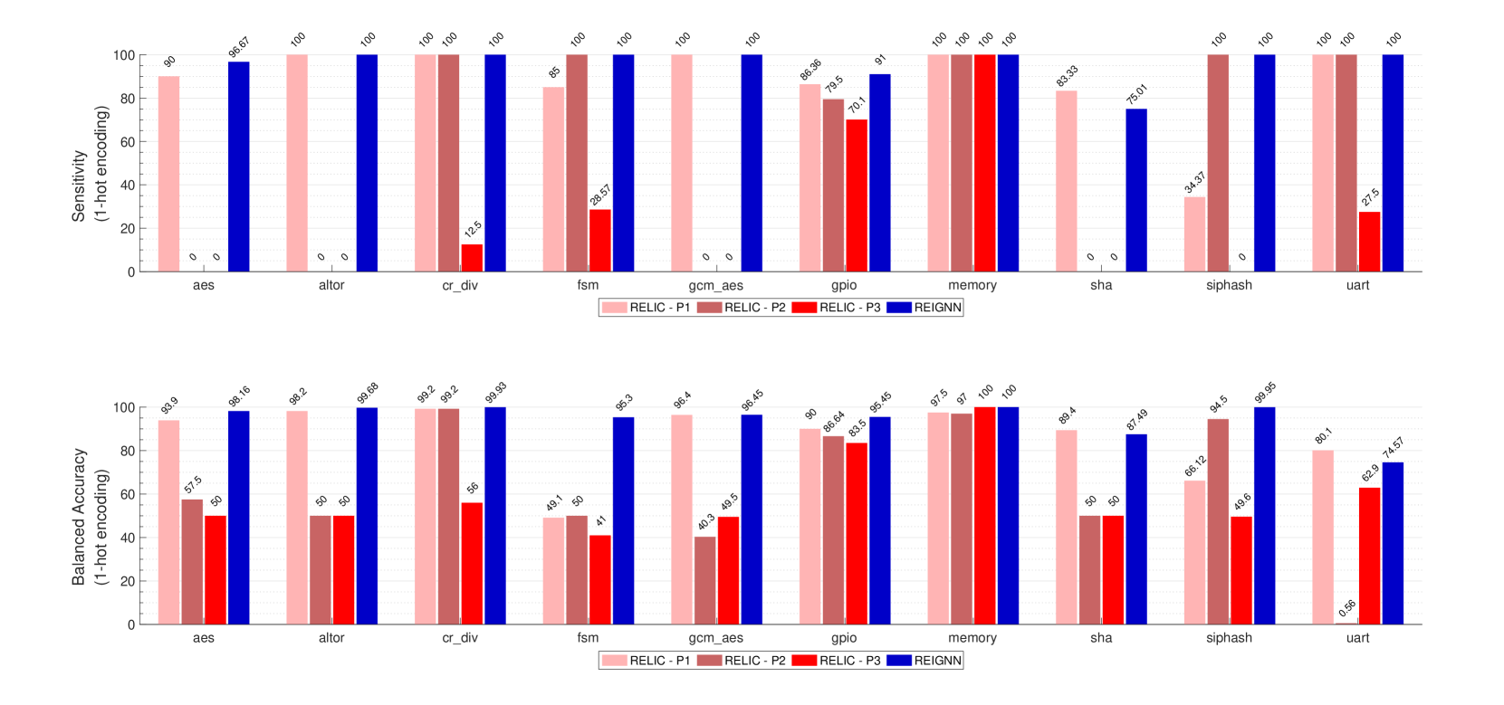
Figure 4: Performance comparison between ReIGNN and RELIC on one-hot encoded benchmarks.

V-3 Evaluation Method and Metrics

We perform classification tasks on an independent set of netlists, which excludes the ones used for training and validation. Specifically, we use k-fold cross validation [52], where the data is initially divided into k bins and the model is trained using k-1 bins and tested on the k-th bin. This process is repeated k times and each time a new bin is considered as the test set. In our case, the $4$ different versions of a design create the test set each time. For example, when reporting the performance on the $aes$ benchmark in the one-hot encoded dataset, $4$ different $aes$ graphs create the test set, $80\%$ of the remaining graphs in the dataset are used for training, while the rest are used for validation. To evaluate the performance of ReIGNN, we compare its predictions with the true labels of the nodes and use the standard statistical measures of correctness of a binary classification test. Since the dataset is imbalanced, we use sensitivity, or true positive rate (TPR), specificity, or true negative rate (TNR), and balanced accuracy as the metrics, defined as follows:

$$\text{Sensitivity}=\frac{\text{No. true positives}}{\text{No. true positives + No. false negatives}},$$ (6)

$$\text{Specificity}=\frac{\text{No. true negatives}}{\text{No. true negatives + No. false positives}},$$ (7)

$$\text{Balanced Accuracy}=\frac{\text{Sensitivity + Specificity}}{\text{2}},$$ (8)

where we consider detecting state registers as positive outcomes and data registers as negative outcomes. Therefore, a true positive (TP) implies that a state register is correctly identified as a state register by ReIGNN, while a false positive (FP) means that a data register is incorrectly classified by ReIGNN as a state register. True negatives (TNs) and false negatives (FNs) can also be defined in a similar way. Overall, the sensitivity is the ratio between the number of correctly identified state registers and the total number of state registers in the design. The specificity is the ratio between the number of correctly identified data registers and the total number of data registers. The balanced accuracy is the average of sensitivity and specificity. High sensitivity and high balanced accuracy are both desirable, since they impact any FSM extraction methodology for IC reverse engineering. If we report low sensitivity, then there exist unidentified state registers, which will impact the correctness of the extracted FSM. On the other hand, low specificity, hence low balanced accuracy, makes FSM extraction time consuming since many data registers are also identified as state registers and will be included in the STG of the FSM.

V-4 Performance Analysis

We evaluate the performance of ReIGNN on all the benchmarks from the one-hot encoded and binary encoded datasets. The GNN models are trained offline using the available data, thus incurring a one-time-only training cost. The average test time of the trained model is $1$ s while the average training time is $8500$ s. For each benchmark, Fig. 4 shows the average balanced accuracy and sensitivity across the $4$ different synthesized versions of the netlist. We compare the achieved performance with the one of RELIC [14], which has a similar classification accuracy as fastRELIC [15]. In fact, while fastRELIC reduces the run-time of RELIC, it uses the same heuristic for determining the similarity scores between two registers. In RELIC, the user needs to set the three threshold values $T1$, $T2$, and $T3$ together with the fan-in cone depth d. In our experiments, we consider the following parameter configurations, which are also used in the literature:

• P1: $T1$ = 0.5, $T2$ = 0.8, $T3$ = 1, d = 5;

• P2: $T1$ = 0.7, $T2$ = 0.5, $T3$ = 5, d = 5;

• P3: $T1$ = 0.4, $T2$ = 0.5, $T3$ = 4, d = 7.

Depending on the threshold values, both balanced accuracy and sensitivity vary largely across different benchmarks. Across the one-hot encoded benchmarks, ReIGNN reports an average balanced classification accuracy of $94.7\%$ and a sensitivity of $96.3\%$. RELIC’s average balanced accuracy varies between $68.14\%$ (for configuration P2) and $86.6\%$ (for configuration P1) while its sensitivity varies between $23.91\%$ (for configuration P3) and $87.96\%$ (for configuration P1).

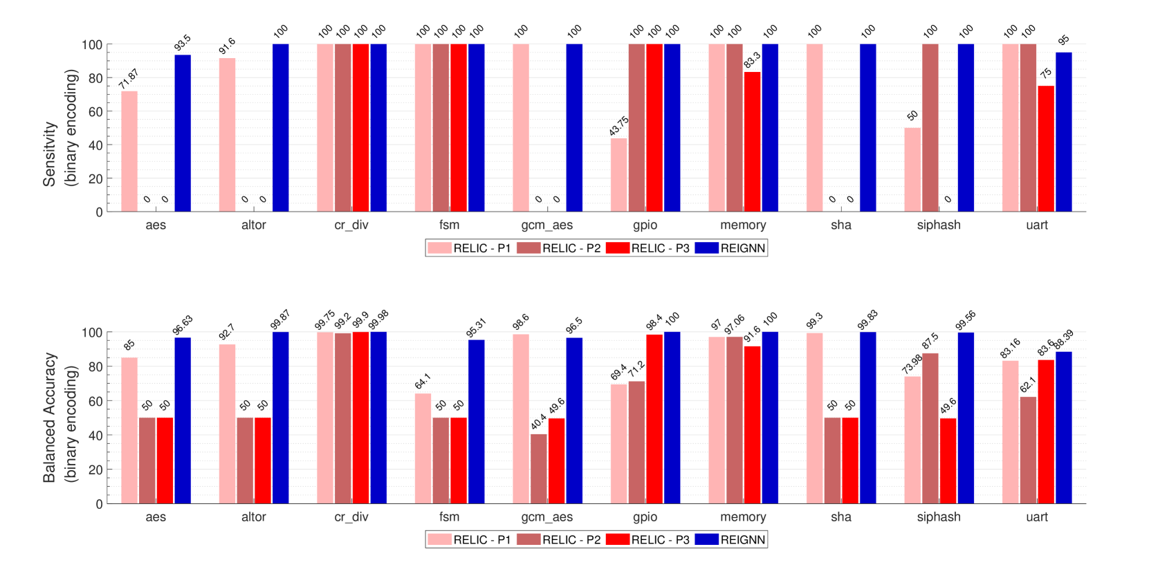
Figure 5: Performance comparison between ReIGNN and RELIC on binary encoded benchmarks.

To analyze the impact of the performance of different tools, we consider, for instance, the $aes$ benchmark, including a total of $2994$ registers, only $15$ of which are state registers. As shown in Fig. 4, across the four synthesized versions of the netlist, ReIGNN achieves on average a balanced accuracy of $98.16\%$ (FP = $11,11,10,9$ for the four netlists) and a sensitivity of $96.67\%$. Specifically, the sensitivity is $100\%$ (TP = $15$, FN = $0$) for two designs and decreases to $93.33\%$ (TP = $14$, FN = $1$) for the other two. On the other hand, when using configuration P1, the average accuracy of RELIC is $93.9\%$ with FP values of $71$, $67$, $55$, and $69$. RELIC achieved a sensitivity of $80\%$ for two netlists (TP = $12$, FN = $3$) and $93.33\%$ (TP = $14$, FN = $1$) and $100\%$ (TP = $15$, FN = $0$) on the other two. Overall, Algorithm 1 produces more FPs, which can make the FSM extraction task harder.

Whenever ReIGNN cannot achieve full sensitivity, meaning that some state registers are misclassified as data registers, we can still use structural analysis to bring the number of FNs to zero. In fact, by finding the SCCs associated with the correctly classified state registers, we can look for all the registers that are part of the SCCs, some of which may indeed be data registers, and label them as state registers for FSM extraction. This extension makes ReIGNN complete (TN = $0$) but compromises its soundness (FP $\neq 0$), which, again, may increase the complexity of the FSM extraction. Finally, when using configuration P2 and P3, Algorithm 1 has $0\%$ sensitivity, meaning that all state registers are misclassified and it is not possible to recover the FSM. As shown in Fig. 4, ReIGNN can achieve an average sensitivity of $100\%$ for uart but the average balanced accuracy is only $74.57\%$, implying that the number of FPs is high. This is due to the fact that the registers associated with the counters in the design are all classified as state registers by the GNN. Moreover, since these registers are all part of an SCC, structural analysis cannot help rectify these misclassifications. While a counter is indeed an FSM, by our definition, its registers are data registers, in that they do not hold the state bits of the control logic FSM. This explains the lower performance of ReIGNN.

Across the binary encoded benchmarks, ReIGNN reports an average balanced accuracy of $97.9\%$ and a sensitivity of $99.4\%$. RELIC’s average balanced accuracy varies between $66.4\%$ (for configuration P2) and $86.6\%$ (for configuration P1) while its sensitivity varies between $45.8\%$ (for configuration P3) and $85.72\%$ (for configuration P1) as shown in Fig. 5. In general, structural analysis has a considerable impact on the overall performance of ReIGNN. While the sensitivity remains unchanged, as explained in Section IV-C, the average balanced accuracy can substantially improve, e.g., by $6.52\%$, as shown in Table III, for the one-hot encoded benchmarks. While the application of structural analysis does not bring large improvements for designs like uart and gcm_aes, due to the presence of the counters, the balanced accuracy improves by $32.3\%$, $12.15\%$, and $11.3\%$ for designs like fsm, gpio, and memory, respectively.

TABLE III: Analysis of the balanced accuracy change in ReIGNN due to inclusion of structural analysis

Design	Balanced Accuracy(GNN only)	Balanced Accuracy(GNN & SCC)
aes	97.05%	98.16%
altor32_lite	98.43%	99.68%
cr_div	98.5%	99.93%
fsm	63%	95.3%
gcm_aes	91.3%	96.45%
gpio	83.3%	95.45%
memory	88.3%	100%
sha	84.2%	87.49%
siphash	94.45%	99.95%
uart	73.3%	74.57%

Finally, to see how well ReIGNN generalizes across different types of benchmarks and encoding styles, we create a dataset with both one-hot encoded and binary-encoded versions of each benchmark, for a total of $80$ graphs. Similarly to our previous experiments, we perform classification tasks on each benchmark independently. As shown in Table IV, ReIGNN generalizes well across different encoding styles and achieves on average a balanced classification accuracy of $96.93\%$ and a sensitivity of $97.53\%$.

TABLE IV: Performance of ReIGNN for combined dataset

Design	Sensitivity	Balanced Accuracy
aes	100%	99.69%
altor32_lite	100%	99.49%
cr_div	100%	99.99%
fsm	100%	93.75%
gcm_aes	100%	96.76%
gpio	92.04%	96.02%
memory	100%	100%
sha	89.58%	99.94%
siphash	100%	99.9%
uart	93.75%	83.74%

VI Conclusions

We presented ReIGNN, a learning-based register classification methodology for finite state machine extraction and circuit reverse engineering. ReIGNN combines graph neural networks with structural analysis to classify the registers in a circuit with high accuracy and generalize well across different designs. Numerical results show the advantage of combining graph-based deep learning with post-processing based on structural analysis to achieve higher balanced accuracy and sensitivity with respect to previous classification methods. Future work includes further investigation of the proposed architecture to possibly reduce its complexity and the number of features for the same performance.

References

- [1] D. Board, “Defense Science Board (DSB) study on high performance microchip supply,” URL www. acq. osd. mil/dsb/reports/ADA435563. pdf,[March 16, 2015], 2005.
- [2] S. E. Quadir, J. Chen, D. Forte, N. Asadizanjani, S. Shahbazmohamadi, L. Wang, J. Chandy, and M. Tehranipoor, “A survey on chip to system reverse engineering,” ACM Journal on Emerging Technologies in Computing Systems (JETC), vol. 13, no. 1, pp. 1–34, 2016.
- [3] U. Guin, K. Huang, D. DiMase, J. M. Carulli, M. Tehranipoor, and Y. Makris, “Counterfeit integrated circuits: A rising threat in the global semiconductor supply chain,” Proceedings of the IEEE, vol. 102, no. 8, pp. 1207–1228, 2014.
- [4] M. Tehranipoor and F. Koushanfar, “A survey of hardware Trojan taxonomy and detection,” IEEE Design & Test of Computers, vol. 27, no. 1, pp. 10–25, 2010.
- [5] R. Torrance and D. James, “The state-of-the-art in IC reverse engineering,” in International Workshop on Cryptographic Hardware and Embedded Systems, pp. 363–381, Springer, 2009.
- [6] J. Baehr, A. Bernardini, G. Sigl, and U. Schlichtmann, “Machine learning and structural characteristics for reverse engineering,” Integration, vol. 72, pp. 1–12, 2020.
- [7] A. Gascón, P. Subramanyan, B. Dutertre, A. Tiwari, D. Jovanović, and S. Malik, “Template-based circuit understanding,” in Formal Methods in Computer-Aided Design (FMCAD), pp. 83–90, IEEE, 2014.
- [8] W. Li, Z. Wasson, and S. A. Seshia, “Reverse engineering circuits using behavioral pattern mining,” in IEEE International Symposium on Hardware-Oriented Security and Trust (HOST), pp. 83–88, 2012.
- [9] A. Fayyazi, S. Shababi, P. Nuzzo, S. Nazarian, and M. Pedram, “Deep learning-based circuit recognition using sparse mapping and level-dependent decaying sum circuit representations,” in Design, Automation & Test in Europe Conference & Exhibition (DATE), pp. 638–641, 2019.
- [10] Y. Shi, C. W. Ting, B.-H. Gwee, and Y. Ren, “A highly efficient method for extracting FSMs from flattened gate-level netlist,” in Proceedings of IEEE International Symposium on Circuits and Systems, pp. 2610–2613, 2010.
- [11] K. S. Mcelvain, “Methods and apparatuses for automatic extraction of finite state machines,” Jan. 30 2001. US Patent 6,182,268.
- [12] T. Meade, S. Zhang, and Y. Jin, “Netlist reverse engineering for high-level functionality reconstruction,” in 21st Asia and South Pacific Design Automation Conference (ASP-DAC), pp. 655–660, 2016.
- [13] M. Fyrbiak, S. Wallat, J. Déchelotte, N. Albartus, S. Böcker, R. Tessier, and C. Paar, “On the difficulty of FSM-based hardware obfuscation,” IACR Transactions on Cryptographic Hardware and Embedded Systems, pp. 293–330, 2018.
- [14] T. Meade, Y. Jin, M. Tehranipoor, and S. Zhang, “Gate-level netlist reverse engineering for hardware security: Control logic register identification,” in IEEE International Symposium on Circuits and Systems (ISCAS), pp. 1334–1337, 2016.
- [15] M. Brunner, J. Baehr, and G. Sigl, “Improving on state register identification in sequential hardware reverse engineering,” in IEEE International Symposium on Hardware Oriented Security and Trust (HOST), pp. 151–160, 2019.
- [16] J. Geist, T. Meade, S. Zhang, and Y. Jin, “RELIC-FUN: logic identification through functional signal comparisons,” in 57th ACM/IEEE Design Automation Conference (DAC), pp. 1–6, 2020.
- [17] T. Meade, K. Shamsi, T. Le, J. Di, S. Zhang, and Y. Jin, “The old frontier of reverse engineering: Netlist partitioning,” Journal of Hardware and Systems Security, vol. 2, no. 3, pp. 201–213, 2018.
- [18] P. Subramanyan, N. Tsiskaridze, K. Pasricha, D. Reisman, A. Susnea, and S. Malik, “Reverse engineering digital circuits using functional analysis,” in Design, Automation & Test in Europe Conference & Exhibition (DATE), pp. 1277–1280, 2013.
- [19] P. Subramanyan, N. Tsiskaridze, W. Li, A. Gascón, W. Y. Tan, A. Tiwari, N. Shankar, S. A. Seshia, and S. Malik, “Reverse engineering digital circuits using structural and functional analyses,” IEEE Transactions on Emerging Topics in Computing, vol. 2, no. 1, pp. 63–80, 2013.
- [20] Z. Huang, Q. Wang, Y. Chen, and X. Jiang, “A survey on machine learning against hardware Trojan attacks: Recent advances and challenges,” IEEE Access, vol. 8, pp. 10796–10826, 2020.
- [21] R. Yasaei, S.-Y. Yu, and M. A. Al Faruque, “GNN4TJ: Graph neural networks for hardware Trojan detection at register transfer level,” in Design, Automation & Test in Europe Conference & Exhibition (DATE), pp. 1504–1509, 2021.
- [22] Y. Hu, K. Yang, S. D. Chowdhury, and P. Nuzzo, “Risk-aware cost-effective design methodology for integrated circuit locking,” in Design, Automation & Test in Europe Conference & Exhibition (DATE), pp. 1182–1185, 2021.
- [23] S. D. Chowdhury, G. Zhang, Y. Hu, and P. Nuzzo, “Enhancing SAT-attack resiliency and cost-effectiveness of reconfigurable-logic-based circuit obfuscation,” in IEEE International Symposium on Circuits and Systems (ISCAS), pp. 1–5, 2021.
- [24] D. Sisejkovic, F. Merchant, L. M. Reimann, H. Srivastava, A. Hallawa, and R. Leupers, “Challenging the security of logic locking schemes in the era of deep learning: A neuroevolutionary approach,” ACM Journal on Emerging Technologies in Computing Systems (JETC), vol. 17, no. 3, pp. 1–26, 2021.
- [25] P. Chakraborty, J. Cruz, and S. Bhunia, “SAIL: Machine learning guided structural analysis attack on hardware obfuscation,” in Asian Hardware Oriented Security and Trust Symposium (AsianHOST), pp. 56–61, 2018.
- [26] L. Alrahis, S. Patnaik, F. Khalid, M. A. Hanif, H. Saleh, M. Shafique, and O. Sinanoglu, “GNNUnlock: Graph neural networks-based oracle-less unlocking scheme for provably secure logic locking,” in Design, Automation & Test in Europe Conference & Exhibition (DATE), pp. 780–785, 2021.
- [27] J. L. Hennessy and D. A. Patterson, Computer architecture: a quantitative approach. Elsevier, 2011.
- [28] Y. LeCun, Y. Bengio, et al., “Convolutional networks for images, speech, and time series,” The Handbook of Brain Theory and Neural Networks, vol. 3361, no. 10, p. 1995, 1995.
- [29] S. Hochreiter and J. Schmidhuber, “Long short-term memory,” Neural Computation, vol. 9, no. 8, pp. 1735–1780, 1997.
- [30] R. Girshick, J. Donahue, T. Darrell, and J. Malik, “Rich feature hierarchies for accurate object detection and semantic segmentation,” in Proceedings of the IEEE Conference on Computer Vision and Pattern Recognition, pp. 580–587, 2014.
- [31] K. He, X. Zhang, S. Ren, and J. Sun, “Deep residual learning for image recognition,” in Proceedings of the IEEE Conference on Computer Vision and Pattern Recognition, pp. 770–778, 2016.
- [32] J. Redmon, S. Divvala, R. Girshick, and A. Farhadi, “You only look once: Unified, real-time object detection,” in Proceedings of the IEEE Conference on Computer Vision and Pattern Recognition, pp. 779–788, 2016.
- [33] T. Young, D. Hazarika, S. Poria, and E. Cambria, “Recent trends in deep learning based natural language processing,” IEEE Computational Intelligence Magazine, vol. 13, no. 3, pp. 55–75, 2018.
- [34] G. Hinton, L. Deng, D. Yu, G. E. Dahl, A.-r. Mohamed, N. Jaitly, A. Senior, V. Vanhoucke, P. Nguyen, T. N. Sainath, et al., “Deep neural networks for acoustic modeling in speech recognition: The shared views of four research groups,” IEEE Signal Processing Magazine, vol. 29, no. 6, pp. 82–97, 2012.
- [35] W. L. Hamilton, “Graph representation learning,” Synthesis Lectures on Artificial Intelligence and Machine Learning, vol. 14, no. 3, pp. 1–159, 2020.
- [36] Z. Wu, S. Pan, F. Chen, G. Long, C. Zhang, and S. Y. Philip, “A comprehensive survey on graph neural networks,” IEEE Transactions on Neural Networks and Learning Systems, vol. 32, no. 1, pp. 4–24, 2020.
- [37] J. Gilmer, S. S. Schoenholz, P. F. Riley, O. Vinyals, and G. E. Dahl, “Neural message passing for quantum chemistry,” in International Conference on Machine Learning, pp. 1263–1272, PMLR, 2017.
- [38] T. N. Kipf and M. Welling, “Semi-supervised classification with graph convolutional networks,” arXiv preprint arXiv:1609.02907, 2016.
- [39] W. L. Hamilton, R. Ying, and J. Leskovec, “Inductive representation learning on large graphs,” in Proceedings of the 31st International Conference on Neural Information Processing Systems, pp. 1025–1035, 2017.
- [40] M. Zhang and Y. Chen, “Link prediction based on graph neural networks,” Advances in Neural Information Processing Systems, vol. 31, pp. 5165–5175, 2018.
- [41] M. Zhang, Z. Cui, M. Neumann, and Y. Chen, “An end-to-end deep learning architecture for graph classification,” in Thirty-Second AAAI Conference on Artificial Intelligence, 2018.
- [42] R. Ying, J. You, C. Morris, X. Ren, W. L. Hamilton, and J. Leskovec, “Hierarchical graph representation learning with differentiable pooling,” arXiv preprint arXiv:1806.08804, 2018.
- [43] U. Brandes, “On variants of shortest-path betweenness centrality and their generic computation,” Social Networks, vol. 30, no. 2, pp. 136–145, 2008.
- [44] P. Boldi and S. Vigna, “Axioms for centrality,” Internet Mathematics, vol. 10, no. 3-4, pp. 222–262, 2014.
- [45] R. Tarjan, “Depth-first search and linear graph algorithms,” SIAM Journal on Computing, vol. 1, no. 2, pp. 146–160, 1972.
- [46] M. Fey and J. E. Lenssen, “Fast graph representation learning with PyTorch Geometric,” arXiv preprint arXiv:1903.02428, 2019.
- [47] Oliscience, “OpenCores.” [Online], Available: https://opencores.org/projects.
- [48] J. Strombergson, “secworks.” [Online], Available: https://github.com/secworks?tab=repositories.
- [49] “onchipuis.” [Online], Available: https://github.com/onchipuis?tab=repositories.
- [50] “Silvaco: 45nm open cell library (2019).”
- [51] N. Srivastava, G. Hinton, A. Krizhevsky, I. Sutskever, and R. Salakhutdinov, “Dropout: a simple way to prevent neural networks from overfitting,” Journal of Machine Learning Research (JMLR), vol. 15, no. 1, pp. 1929–1958, 2014.
- [52] R. Kohavi, “A study of cross-validation and bootstrap for accuracy estimation and model selection,” in Proceedings of the 14th International Joint Conference on Artificial Intelligence - Volume 2, IJCAI’95, pp. 1137––1143, 1995.