Galactic Winds across the Gas-Rich Merger Sequence.
I. Highly
Ionized N V and O VI Outflows in the QUEST Quasars 111Based on
observations made with the NASA/ESA Hubble Space Telescope,
obtained from the data archive at the Space Telescope Science
Institute. STScI is operated by the Association of Universities
for Research in Astronomy, Inc. under NASA contract NAS 5-26555.
Abstract
This program is part of QUEST (Quasar/ULIRG Evolutionary Study) and seeks to examine the gaseous environments of quasars and ULIRGs as a function of host galaxy properties and age across the merger sequence from ULIRGs to quasars. This first paper in the series focuses on 33 quasars from the QUEST sample and on the kinematics of the highly ionized gas phase traced by the N V 1238,1243 and O VI 1032,1038 absorption lines in high-quality Hubble Space Telescope (HST) Cosmic Origins Spectrograph (COS) data. N V and O VI outflows are present in about 60% of the QUEST quasars and span a broad range of properties, both in terms of equivalent widths (from 20 mÅ to 25 Å) and kinematics (outflow velocities from a few 100 km s-1 up to 10,000 km s-1). The rate of incidence and equivalent widths of the highly ionized outflows are higher among X-ray weak or absorbed sources. The weighted outflow velocity dispersions are highest among the X-ray weakest sources. No significant trends are found between the weighted outflow velocities and the properties of the quasars and host galaxies although this may be due to the limited dynamic range of properties of the current sample. These results will be re-examined in an upcoming paper where the sample is expanded to include the QUEST ULIRGs. Finally, a lower limit of 0.1% on the ratio of time-averaged kinetic power to bolometric luminosity is estimated in the 24 objects with blueshifted P V 1117,1128 absorption features.
1 Introduction
Large multiwavelength surveys of the local and distant universe have shown that major mergers of gas-rich galaxies222In this paper, we define major mergers as those involving galaxies with 4:1 stellar mass ratios. may trigger spectacular bursts of star formation, accompanied with quasar-like episodes of rapid growth of the supermassive black holes (SMBHs), and result in merger remnants that follow tight SMBH-host scaling relations and resemble today’s quiescent early-type galaxies (e.g. Sanders et al., 1988; Hickox & Alexander, 2018). Modern simulations of galaxy formation and evolution (e.g. Nelson et al., 2019; Oppenheimer et al., 2020; Nelson et al., 2021) largely reproduce these observations. However, the root cause of the fast “quenching” of the star formation activity in the merger remnants depends on the detailed, sub-grid scale, implementation of how the mass, momentum, and energy from stellar winds, supernova explosions, and SMBH-related processes are injected into, and interact with, the interstellar medium (ISM) and circumgalactic medium (CGM) of the host galaxies. Over the past several years, nearby gas-rich galaxy mergers have emerged as excellent laboratories to study in detail these stellar and quasar feedback processes (see Veilleux et al., 2020, for a recent review). These objects are the focus of the present study.
Locally, major gas-rich galaxy mergers often coincide with obscured ultraluminous infrared galaxies (ULIRGs). As these systems evolve, the obscuring gas and dust, funneled to the center by the dissipative collapse and tidal forces during the merger, are either transformed into stars or expelled out of the nucleus by powerful winds driven by the central quasar and starburst, giving rise to dusty quasars and finally to completely exposed quasars. Galactic-scale winds are ubiquitous in local ULIRGs and dusty quasars (e.g. Sturm et al., 2011; Veilleux et al., 2013a; Cicone et al., 2014; Rupke et al., 2017; Veilleux et al., 2017; Fluetsch et al., 2019, 2020; Lutz et al., 2020; Veilleux et al., 2020, and references therein). The outflows detected in ULIRGs extend over a large range of distances from the central energy source, seamlessly blending with the circumgalactic medium at 10 kpc (Veilleux et al., 2020, and references therein).
In these objects, the outflow masses and energetics are often dominated by the outer (kpc) cool dusty molecular or neutral atomic gas phase, but the driving mechanism is best probed by examining the inner ( sub-kpc) ionized phase. ULIRG F111193257 is the first and still the best case among local ULIRGs where a fast (0.1 c), highly ionized (Fe XXV/XXVI at 7 keV), accretion-disk scale (1 pc) quasar wind appears to be driving a massive ( 100 yr-1), large-scale (110+ kpc) molecular and neutral-gas outflow (Tombesi et al., 2015, 2017; Veilleux et al., 2017). Unfortunately, the search for hot winds in a statistically significant sample of ULIRGs is not feasible at present since most ULIRGs are too faint at 7 keV for current X-ray observatories.
This is where the excellent far-ultraviolet (FUV) spectroscopic sensitivity of the Hubble Space Telescope (HST) becomes handy. The FUV band is rich in spectroscopic diagnostics of the neutral, low-ionization, and high-ionization gas phases (Haislmaier et al., 2021); thus HST can probe all three phases at once. So far, only about a dozen ULIRGs and IR-bright quasars have been studied with HST, but the results have been promising. Prominent, blueshifted Ly emission out to 1000 km s-1 has been detected in half of these ULIRGs. Blueshifted absorption features from high-ionization species like N V and O VI (77 and 114 eV are needed to produce N4+ and O5+ ions, respectively) and/or low-ionization species like Si II, Si III, Fe II, N II, and Ar I have provided additional unambiguous signatures of outflows in a few of these objects. Martin et al. (2015) have argued that the FUV-detected outflows represent clumps of gas condensing out of a fast, hot wind generated by the central starburst (Thompson et al., 2016). This picture is also consistent with the blast-wave model for quasar feedback. In this model, a fast, hot wind shocks the surrounding ISM, which then eventually cools to reform the molecular gas after having acquired a significant fraction of the initial kinetic energy of the hot wind (e.g. Weymann et al., 1985; Zubovas & King, 2012, 2014; Faucher-Giguère & Quataert, 2012; Nims et al., 2015; Richings & Faucher-Giguère, 2018a, b; Richings et al., 2021; Girichidis et al., 2021). An alternative explanation is radiative acceleration (e.g. Ishibashi et al., 2018, 2021), which may dominate the dynamics of outflows on a wide variety of scales (e.g. Stern et al., 2016; Revalski et al., 2018; Somalwar et al., 2020).
So far, the published data set on ULIRGs and IR-bright quasars is too small to draw strong conclusions about the properties of the FUV-detected winds. There is tantalizing evidence that UV-detected AGN/starburst-driven winds are present in most ULIRGs, but the sample is very incomplete, particularly among ULIRGs with AGN and matched quasars. A more diverse sample of ULIRGs and quasars is needed to study the gaseous environments of nearby quasars and ULIRGs as a function of host properties and age across the merger sequence from ULIRGs to quasars. This issue is addressed in the present study.
In this first paper, we focus our efforts on studying the highly ionized gas, traced by N V 1238, 1243 and O VI 1032, 1038, in a sample of 33 local quasars, while Paper II (Liu et al. 2021, in prep.) will present the results on our sample of ULIRGs with AGN and compare them with those on the quasars. As stated in Hamann et al. (2019b), the quasars in the present sample are valuable for outflow studies in and of themselves because: 1) they fill a largely-unexplored niche between luminous quasars with strong broad absorption lines (BALs) with outflow velocities of up to 0.1 0.2 and low-luminosity Seyfert 1 galaxies with exclusively narrower outflow lines, 2) their low redshift minimizes contamination by the Ly forest, and 3) the outflow lines are relatively narrow so blending is less severe. Indeed, as we discuss below, the detected outflows often are “mini-BALs” instead of BALs because their velocity widths lie below or near the threshold of 2000 km s-1 used for BALs (Weymann et al., 1981, 1991; Hamann & Sabra, 2004; Gibson et al., 2009b).
Our quasar sample is discussed in Section 2. The extensive set of ancillary data on these quasars is summarized in Section 3. The HST spectra used for this study are described in Section 4 and the methods applied to analyze these data are detailed in Section 5. The results from this analysis are presented in Section 6, and discussed in more detail in Section 7. Section 8 provides a summary of the main results from this paper.
2 Quasar Sample
The quasars in our sample are selected using four criteria: (1) They must be part of the QUEST (Quasar/ULIRG Evolutionary Study) sample of local () ULIRGs and quasars. The QUEST sample has already been described in detail in Veilleux et al. (2009a, b) and references therein. All 33 objects in the present sample are Palomar-Green (PG) quasars from the Bright Quasar Sample (Schmidt & Green, 1983), except Mrk 231, the nearest quasar known, whose UV spectrum has already been analyzed by Veilleux et al. (2013b, 2016) and will not be discussed here any further. As part of the QUEST sample, the quasars are carefully matched in terms of redshifts, bolometric luminosities, and host galaxy masses with the QUEST ULIRGs of Paper II. (2) Their bolometric luminosity must be quasar-like, ergs s-1, and dominated by the quasar rather than the starburst based on the Spitzer data (see criterion #3 below) or, equivalently, have 25-to-60 m flux ratios (Veilleux et al., 2009a). This criterion also automatically selects UV-detected late-stage mergers or non-mergers (Veilleux et al., 2009b). (3) A strong preference is also given to the QUEST quasars with Spitzer mid-infrared spectra to provide valuable information on the AGN contribution to the bolometric luminosities of these objects. (4) High-quality COS spectra covering systemic N V and/or O VI must exist for each object in the sample. Only COS data are considered to ease comparisons between spectra and avoid possible systematic errors associated with comparing data sets from different instruments. As described in Section 4, both our own and archival data are used for this study.
These criteria result in a sample of 33 objects. Table 3 lists the key properties of the quasars in our sample, many of which are derived from our extensive set of ancillary data on these objects, discussed in Section 3. As shown in Figure 1, these quasars cover the low-redshift and low bolometric luminosity ends of the PG quasar sample. They are well matched in redshift with the QUEST ULIRGs which will be studied in Paper II (Liu et al. 2021, in prep), and are representative of the entire PG quasars sample in terms of infrared excess (defined here as the infrared-to-bolometric luminosity ratio, ) and FIR brightness ( from Netzer et al., 2007).
3 Ancillary Data
An extensive set of spectroscopic and photometric data exist on all of the objects in the sample. Sloan Digital Sky Survey (SDSS) optical spectra are available for all of them. High-quality optical spectra also exist in Boroson & Green (1992), and Krug (2013) presents spectra centered on Na I D 5890, 5896. As mentioned in Section 2, most of these quasars have also been studied spectroscopically in the mid-infrared with Spitzer (Schweitzer et al., 2006, 2008; Netzer et al., 2007; Veilleux et al., 2009a). In addition, nearly all of the quasars in this sample are part of X-QUEST, an archival XMM-Newton and Chandra X-ray spectroscopic survey of the QUEST sample (Teng & Veilleux 2010; Columns 13-17 in Table 3). VLT and Keck near-infrared spectroscopic data exist for a number of these objects (Dasyra et al., 2007).
Optical and near-infrared images of these objects have been obtained from the ground (Surace et al., 2001; Veilleux et al., 2002; Guyon et al., 2006) and with HST (Veilleux et al., 2006; Kim et al., 2008; Hamilton et al., 2008; Veilleux et al., 2009b), providing photometric and morphological measurements on both the quasars and host galaxies (e.g., morphological type, quasar-to-host luminosity ratio, strength of tidal features). Far-infrared photometry obtained with the Herschel PACS instrument exists for all of these objects (Lani et al., 2017; Shangguan et al., 2018), while far-infrared spectra centered on the OH 119 m feature exist for five of them (Veilleux et al., 2013a). Finally, Green Bank Telescope (GBT) H I 21-cm line emission and absorption spectra are available for 16 of these quasars (Teng et al., 2013).
The connection between UV and X-ray properties is critical, so we searched the literature for additional X-ray measurements (ignoring older ones from ROSAT/ASCA). These are listed and referenced in Table 3. For Chandra observations from Teng & Veilleux (2010) where no absorbing column was detected, more recent constraints from Ricci et al. (2017) (based on Swift/BAT detections) are available in some cases. In these cases, we substitute the newer measurement of absorbing column.
=0.25in
| Name | Other | log Lν(UV) | log | Radio | log() | log() | log() | log | log() | log() | Ref. | |||||
|---|---|---|---|---|---|---|---|---|---|---|---|---|---|---|---|---|
| Name | [erg s-1] | Class | [erg s-1] | [erg s-1] | [1022 cm-2] | |||||||||||
| PG 0007106 | III Zw 2 | 0.0893 | 44.55 | 2.29 | Flat | 1.43 | 12.24 | 1aaNo measurement; we assume a value of 1. | 11.63 | 8.07 | 0.34 | 43.94 | 44.18 | 1.73 | 0.11 | a, 4, 5 |
| PG 0026129 | … | 0.1454 | 45.32 | 0.03 | Quiet | 1.50 | 12.08 | 0.986 | 11.71 | 8.49 | 0.93 | 44.40 | 2.00 | 0.01 | g, 5 | |
| PG 0050124 | I Zw 1 | 0.0589 | 44.24 | 0.48 | Quiet | 1.56 | 12.08 | 0.925 | 12.04 | 7.33 | 0.20 | 44.04 | 43.88 | 2.25 | 0.09 | f, 6 |
| 43.78 | 43.64 | 2.09 | 0.04 | 6 | ||||||||||||
| 43.633 | 2.37 | 0.045 | 3 | |||||||||||||
| PG 0157001 | Mrk 1014 | 0.1633 | 45.34 | 0.33 | Quiet | 1.60 | 12.70 | 0.727 | 12.67 | 8.06 | 0.01 | 43.92 | 43.83 | 2.54 | 0.009 | e, 3, 6 |
| 44.00 | 43.86 | 2.1 | 0.009 | 3, 6 | ||||||||||||
| PG 0804761 | … | 0.100 | 45.54 | 0.22 | Quiet | 1.52 | 12.09 | 0.996 | 11.98 | 8.73 | 1.16 | 44.54 | 44.45 | 2.27 | 0.044 | a |
| PG 0838770 | VII Zw 244 | 0.1324 | 44.83 | 0.96 | Quiet | 1.54 | 11.77 | 0.945 | 11.66 | 8.05 | 0.82 | 44.152 | 43.54 | 1.49 | 0.1bbBest-fit value is 0; we assume an upper limit of 1021 cm-2. | d, 4, 5 |
| PG 0844349 | … | 0.064 | 44.59 | 1.52 | Quiet | 1.54 | 11.45 | 0.971 | 11.18 | 7.86 | 0.94 | 44.152 | 43.80 | 2.66 | 6.13 | a, 6 |
| PG 0923201 | … | 0.192 | 45.42 | 0.85 | Quiet | 1.57 | 12.46 | 0.990 | 12.05 | 7.90 | 0.04 | i | ||||
| PG 0953414 | … | 0.2341 | 45.95 | 0.36 | Quiet | 1.50 | 12.53 | 0.982 | 12.20 | 8.33 | 0.33 | 45.037 | 44.81 | 2.44 | 18.52 | h, 6 |
| PG 1001054 | … | 0.1611 | 44.93 | 0.30 | Quiet | 2.13 | 11.87 | 0.836 | 11.66 | 7.63 | 0.35 | 43.00 | 43.08 | 2.01 | 8.09 | e, 6 |
| PG 1004130 | 4C 13.41 | 0.2406 | 45.30 | 2.36 | Steep | 2.01 | 12.69 | 0.963 | 12.22 | 9.16 | 1.01 | 43.48 | 43.76 | 1.67 | 2.99 | e, 6 |
| 43.51 | 43.89 | 1.52 | 1.44 | 6 | ||||||||||||
| PG 1116215 | … | 0.1765 | 45.79 | 0.14 | Quiet | 1.57 | 12.55 | 0.991 | 12.28 | 8.42 | 0.39 | 44.927 | 44.65 | 2.53 | 27.21 | h, 6 |
| 44.922 | 44.65 | 2.49 | 31.61 | 6 | ||||||||||||
| 44.93 | 44.67 | 2.51 | 20.21 | 6 | ||||||||||||
| PG 1126041 | Mrk 1298 | 0.060 | 44.29 | 0.77 | Quiet | 2.13 | 11.53 | 0.962 | 11.52 | 7.64 | 0.65 | 43.04 | 43.11 | 1.95 | 4.66 | a, 6 |
| PG 1211143 | … | 0.0809 | 44.96 | 1.39 | Steep | 1.57 | 11.97 | 1.000 | 11.74 | 7.85 | 0.40 | 44.328 | 43.94 | 2.83 | 12.98 | h, 6 |
| 44.201 | 43.89 | 2.63 | 12.40 | 6 | ||||||||||||
| PG 1226023 | 3C 273 | 0.158 | 46.50 | 3.06 | Flat | 1.47 | 13.03 | 0.949 | 12.80 | 8.41 | 0.08 | 45.491 | 45.742 | 2.07 | 0.01 | a, 5, 6 |
| 45.461 | 45.722 | 1.81 | 0.01 | 5, 6 | ||||||||||||
| 45.591 | 45.820 | 2.28 | 0.01 | 5, 6 | ||||||||||||
| 45.663 | 45.825 | 2.08 | 0.01 | 5, 6 | ||||||||||||
| 45.461 | 45.67 | 2.13 | 0.01 | 5, 6 | ||||||||||||
| 45.544 | 45.941 | 1.96 | 0.01 | 5, 6 | ||||||||||||
| PG 1229204 | Mrk 771 | 0.064 | 44.42 | 0.96 | Quiet | 1.49 | 11.57 | 0.985 | 11.27 | 7.76 | 0.71 | 43.785 | 43.61 | 2.38 | 13.52 | g, 6 |
| Mrk 231 | … | 0.04217 | 42.70 | 1.92 | 12.61 | 0.709 | 12.54 | 8.58 | 0.63 | 42.13 | 42.58 | 1.40 | 9.5 | b, 7, 8 | ||
| 19.4 | 7, 8 | |||||||||||||||
| PG 1302102 | PKS 1302-102 | 0.2784 | 45.83 | 2.27 | Flat | 1.58 | 12.75 | 0.982 | 12.49 | 8.77 | 0.55 | 44.81 | 1.66 | 0.06 | h, 1 | |
| PG 1307085 | … | 0.155 | 45.35 | 1.00 | Quiet | 1.52 | 12.35 | 0.952 | 11.76 | 8.54 | 0.72 | 44.02 | 44.16 | 1.89 | 5.64 | a, 6 |
| PG 1309355 | … | 0.1829 | 45.05 | 1.26 | Flat | 1.71 | 12.32 | 0.870 | 12.05 | 8.24 | 0.49 | 43.87 | 43.88 | 2.19 | 6.02 | i, 6 |
| PG 1351640 | … | 0.0882 | 45.22 | 0.64 | Quiet | 1.78 | 12.05 | 0.779 | 11.87 | 8.72 | 1.30 | 43.398 | 43.23 | 2.42 | 14.61 | h, 6 |
| PG 1411442 | … | 0.0896 | 44.34 | 0.89 | Quiet | 2.03 | 11.79 | 1.000 | 11.66 | 8.54 | 1.27 | 43.60 | 43.41 | 2.41 | 26.29 | h, 6 |
| PG 1435067 | … | 0.129 | 45.12 | 1.15 | Quiet | 1.63 | 11.92 | 0.976 | 11.47 | 8.26 | 0.86 | 44.11 | 43.94 | 2.36 | 0.1bbBest-fit value is 0; we assume an upper limit of 1021 cm-2. | a, 6 |
| PG 1440356 | Mrk 478 | 0.077 | 45.18 | 0.43 | Quiet | 1.38 | 11.81 | 0.836 | 11.76 | 7.36 | 0.15 | 44.33 | 43.74 | 3.02 | 8.92 | a, 6 |
| 44.375 | 43.90 | 2.86 | 14.24 | 6 | ||||||||||||
| 44.299 | 43.74 | 2.98 | 8.225 | 6 | ||||||||||||
| 44.127 | 43.64 | 2.86 | 12.67 | 6 | ||||||||||||
| PG 1448273 | … | 0.065 | 43.78 | 0.60 | Quiet | 1.59 | 11.44 | 0.997 | 11.19 | 6.86 | 0.06 | 43.949 | 43.49 | 2.80 | 16.72 | a, 6 |
| PG 1501106 | Mrk 841 | 0.036 | 44.03 | 0.44 | Quiet | 1.64 | 11.34 | 1.000 | 11.13 | 8.42 | 1.59 | 44.049 | 43.833 | 2.46 | 23.12 | a, 6 |
| 44.090 | 43.845 | 2.50 | 18.66 | 6 | ||||||||||||
| 44.068 | 43.851 | 2.45 | 15.88 | 6 | ||||||||||||
| 43.740 | 43.672 | 2.26 | 13.01 | 6 | ||||||||||||
| 43.623 | 43.65 | 2.11 | 11.48 | 6 | ||||||||||||
| PG 1613658 | Mrk 876 | 0.129 | 45.43 | 0.00 | Quiet | 1.21 | 12.30 | 0.820 | 12.25 | 8.34 | 0.64 | 44.28 | 44.38 | 1.95 | 28.24 | a, 6 |
| 44.44 | 44.43 | 2.12 | 10.45 | 6 | ||||||||||||
| PG 1617175 | Mrk 877 | 0.114 | 44.93 | 0.14 | Quiet | 1.64 | 11.75 | 0.903 | 11.55 | 8.67 | 1.48 | a | ||||
| PG 1626554 | … | 0.133 | 45.17 | 0.96 | Quiet | 1.37 | 11.84 | 0.976 | 10.90 | 8.39 | 1.08 | 44.17 | 44.21 | 2.04 | 0.01 | a, 5, 6 |
| PG 2130099 | II Zw 136 | 0.063 | 44.46 | 0.49 | Quiet | 1.47 | 11.78 | 0.995 | 11.63 | 7.43 | 0.17 | 43.708 | 43.62 | 2.29 | 5.91 | j, 6 |
| PG 2214139 | Mrk 304 | 0.0658 | 44.45 | 1.30 | Quiet | 2.02 | 11.78 | 0.998 | 11.46 | 8.44 | 1.18 | 43.46 | 43.64 | 1.80 | 4.48 | e, 6 |
| PG 2233134 | … | 0.3265 | 45.94 | 0.55 | Quiet | 1.66 | 12.56 | 1aaNo measurement; we assume a value of 1. | 12.33 | 7.93 | 0.12 | 44.52 | 2.41 | 0.01 | e, 2 | |
| PG 2349014 | 4C01.61 | 0.1742 | 45.51 | 12.59 | 0.904 | 11.90 | 9.14 | 1.11 | 44.57 | 1.78 | 0.01 | e, 5 |
Note. — Column (1): Object name. Column (2): Other name. Column (3): Redshifts, with reference listed in Column (17). Where available, redshifts are based on the [O III] narrow line. For 3 quasars, we use H I (de Vaucouleurs et al., 1991; Carilli et al., 1998; Springob et al., 2005) instead; for two, full-spectrum fits to SDSS spectra (Schneider et al., 2010); and for a single case, CO data (Evans et al., 2006). Column (4): Logarithm of the monochromatic luminosity at rest-frame 1125 Å derived using the Galactic extinctions from Schlafly & Finkbeiner (2011) and the reddening curve with of Fitzpatrick (1999). Column (5): logarithm of , the ratio of radio-to-optical luminosity from Boroson & Green (1992). Column (6): Radio class Quiet, Steep, or Flat depending on log and radio spectral index from Boroson & Green (1992). Column (7): X-ray to optical spectral index = 0.372 log () from Brandt et al. (2000), where and are the rest-frame flux densities at 2 keV and 3000 Å, respectively. (For Mrk 231, we report the value from Teng et al. (2014).) Column (8): Bolometric luminosity in solar units calculated from 7 (5100 Å) + (Netzer et al., 2007), where (5100 Å) is the continuum luminosity at 5100 Å rest wavelength and is the 1 1000 m infrared luminosity listed in column (10). We adopt a cosmology of 69.3 km s-1; = 0.287; = 0.713 (WMAP9). Column (9): Fraction of the bolometric luminosity produced by the AGN, i.e. , based on the Spitzer results (Veilleux et al., 2009a). The error bars are computed from the lowest and highest values among the six methods from this paper. Column (10): Logarithm of the 1 1000 m infrared luminosity in solar units from Zhuang et al. (2018), except Mrk 231 (U et al., 2013), PG 1626554 (Lyu et al., 2017), and PG 2349014 (Veilleux et al., 2009b). Column (11): Logarithm of the black hole mass in solar units from reverberation mapping (RM) measurements from The AGN Black Hole Mass Database (Bentz & Katz, 2015) or, if unavailable, single-epoch measurements from Vestergaard & Peterson (2006), normalized down from = 5.5 (Onken et al., 2004) to = 4.3 to match RM scaling. According to Vestergaard & Peterson (2006), single-epoch measurements should have an extra 0.43 error added in quadrature. For PG 2349014, we used the more uncertain photometric measurement of Veilleux et al. (2009b). For 3C 273, we recorded the GRAVITY measurement (Gravity Collaboration et al., 2018). Column (12): Logarithm of the ratio of the bolometric luminosity to the Eddington luminosity. Column (13): Luminosity in the soft X-rays (0.5 2 keV). Column (14): Luminosity of the hard X-rays (2 10 keV). Column (15): Photon index of the best-fit absorbed power-law distribution to the X-ray emission (d/d where is the X-ray photon energy). Column (16): Column density in units of 1022 cm-2. For most data from Teng & Veilleux (2010), this is from the best-fit absorbed power-law. Where this best fit is unabsorbed and Swift/BAT data are available, we substitute from Ricci et al. (2017). For X-ray related quantities, different rows = different observations, dates. Column (17): References for the redshift and X-ray measurements.
References. — Redshift: (a) Boroson & Green 1992; (b) Carilli et al. 1998; (c) de Vaucouleurs et al. 1991; (d) Evans et al. 2006; (e) Hewett & Wild 2010; (f) Ho & Kim 2009; (g) Hu et al. 2020; (h) Marziani et al. 1996; (i) Schneider et al. 2010; (j) Springob et al. 2005; X-ray: (1) Inoue et al. 2007; (2) Jin et al. 2012; (3) Laha et al. 2018; (4) Piconcelli et al. 2005; (5) Ricci et al. 2017; (6) Teng & Veilleux 2010; (7) Teng et al. 2014; (8) Veilleux et al. 2014; (9) Waddell & Gallo 2020

4 HST Data
We obtained high-quality spectra for 19 quasars using the Cosmic Origins Spectrograph (COS) with grating G130M under HST PID 12569 in Cycle 19 (PI Veilleux). We acquired multi-epoch COS/G130M data on PG 1411442 under programs 13451, 14460, and 14885 (PI Hamann). We searched for archival COS/G130M spectra of other quasars in the QUEST sample, as well as for multi-epoch data on the subsample we observed. We found archival data on 14 additional QUEST quasars and recent multi-epoch exposures for three quasars in the subsample first observed in Cycle 19. We list the characteristics of these observations in Table 2.
| Name | Range [Å] | CENWAVE [Å] | texp[s] | Date | PID | PI |
|---|---|---|---|---|---|---|
| PG 0007106 | 1151–1470 | 1309/1327 | 1868 | 2011-12-14 | 12569 | S. Veilleux |
| PG 0026129 | 1133–1451 | 1291/1309 | 1868 | 2011-10-25 | 12569 | S. Veilleux |
| PG 0050124 | 1151–1470 | 1309/1327 | 1868 | 2012-11-01 | 12569 | S. Veilleux |
| 1133–1465 | 1291/1309/1327 | 7621 | 2015-01-20 | 13811 | E. Costantini | |
| PG 0157001 | 1151–1469 | 1309/1327 | 1828 | 2012-01-25 | 12569 | S. Veilleux |
| PG 0804761 | 1136–1458 | 1291/1300/1309/1318 | 5510 | 2010-06-12 | 11686 | N. Arav |
| PG 0838770 | 1136–1458 | 1291/1300/1309/1318 | 8865 | 2009-09-24 | 11520 | J. Green |
| PG 0844349 | 1151–1470 | 1309/1327 | 1900 | 2012-03-06 | 12569 | S. Veilleux |
| PG 0923201 | 1133–1451 | 1291/1309 | 1860 | 2012-03-14 | 12569 | S. Veilleux |
| PG 0953414 | 1136–1458 | 1291/1300/1309/1318 | 4785 | 2011-10-18 | 12038 | J. Green |
| PG 1001054 | 1066–1367 | 1222 | 2068 | 2014-04-04 | 13423 | R. Cooke |
| 1140–1455 | 1291/1300/1309/1318 | 3165 | 2014-06-19 | 13347 | J. Bregman | |
| 1131–1429 | 1291 | 2902 | 2019-03-26 | 15227 | J. Burchett | |
| PG 1004130 | 1133–1451 | 1291/1309 | 4107 | 2011-12-21 | 12569 | S. Veilleux |
| PG 1116215 | 1136–1458 | 1291/1300/1309/1318 | 4677 | 2011-10-25 | 12038 | J. Green |
| PG 1126041 | 1152–1470 | 1309/1327 | 1856 | 2012-04-15 | 12569 | S. Veilleux |
| 901–1200 | 1055 | 1874 | 2014-06-01 | 13429 | M. Giustini | |
| 1171–1467 | 1327 | 1580 | 2014-06-01 | 13429 | M. Giustini | |
| 900–1200 | 1055 | 1874 | 2014-06-12 | 13429 | M. Giustini | |
| 1171–1467 | 1327 | 1580 | 2014-06-12 | 13429 | M. Giustini | |
| 900–1200 | 1055 | 1874 | 2014-06-28 | 13429 | M. Giustini | |
| 1171–1467 | 1327 | 1580 | 2014-06-28 | 13429 | M. Giustini | |
| 901–1200 | 1055 | 1837 | 2015-06-14 | 13836 | M. Giustini | |
| 1171–1468 | 1327 | 1540 | 2015-06-14 | 13429 | M. Giustini | |
| PG 1211143 | 1171–1472 | 1327 | 2320 | 2015-04-14 | 13947 | J. Lee |
| PG 1226023 | 1135–1470 | 1291/1300/1309/1318/1327 | 4002 | 2012-04-22 | 12038 | J. Green |
| PG 1229204 | 1152–1469 | 1309/1327 | 1868 | 2012-04-26 | 12569 | S. Veilleux |
| Mrk 231 | 1152–1472 | 1309/1327 | 12536 | 2011-10-15 | 12569 | S. Veilleux |
| PG 1302102 | 1136–1458 | 1291/1300/1309/1318 | 5979 | 2011-08-16 | 12038 | J. Green |
| PG 1307085 | 1152–1470 | 1309/1327 | 1836 | 2012-06-16 | 12569 | S. Veilleux |
| PG 1309355 | 1133–1451 | 1291/1309 | 1896 | 2011-12-06 | 12569 | S. Veilleux |
| PG 1351640 | 1152–1470 | 1309/1327 | 2108 | 2011-10-21 | 12569 | S. Veilleux |
| PG 1411442 | 1152–1470 | 1309 | 1936 | 2011-10-23 | 12569 | S. Veilleux |
| 941–1241 | 1096 | 4954 | 2015-02-12 | 13451 | F. Hamann | |
| 1152–1453 | 1309 | 1917 | 2015-02-12 | 13451 | F. Hamann | |
| 941–1241 | 1096 | 2407 | 2016-04-16 | 14460 | F. Hamann | |
| 1152–1453 | 1309 | 1954 | 2016-04-16 | 14460 | F. Hamann | |
| 941–1241 | 1096 | 1783 | 2017-06-10 | 14885 | F. Hamann | |
| 1152–1453 | 1309 | 1847 | 2017-06-10 | 14885 | F. Hamann | |
| PG 1435067 | 1133–1451 | 1291/1309 | 1864 | 2012-02-29 | 12569 | S. Veilleux |
| PG 1440356 | 1152–1470 | 1309/1327 | 1924 | 2012-01-26 | 12569 | S. Veilleux |
| PG 1448273 | 1136–1448 | 1291/1309 | 2946 | 2011-06-18 | 12248 | J. Tumlinson |
| PG 1501106 | 1132–1434 | 1291 | 3121 | 2014-07-06 | 13448 | A. Fox |
| PG 1613658 | 1145–1467 | 1300/1309/1318/1327 | 9499 | 2010-04-08 | 11524 | J. Green |
| 1133–1429 | 1291 | 3080 | 2010-04-09 | 11686 | N. Arav | |
| PG 1617175 | 1133–1451 | 1291/1309 | 1844 | 2012-06-16 | 12569 | S. Veilleux |
| PG 1626554 | 1136–1458 | 1291/1300/1309/1318 | 3318 | 2011-06-15 | 12029 | J. Green |
| PG 2130099 | 1135–1458 | 1291/1300/1309/1318 | 5513 | 2010-10-28 | 11524 | J. Green |
| PG 2214139 | 1152–1463 | 1309/1327 | 1401 | 2011-11-08 | 12569 | S. Veilleux |
| 1138–1434 | 1291 | 2082 | 2012-09-21 | 12604 | A. Fox | |
| PG 2233134 | 1171–1472 | 1327 | 2104 | 2014-06-18 | 13423 | R. Cooke |
| PG 2349014 | 1152–1470 | 1309/1327 | 1844 | 2011-10-20 | 12569 | S. Veilleux |
Note. — Column (1): Name of object; Column (2): Wavelength range, in Å; Column (3): CENWAVE setting(s); Column (4): Exposure time, in seconds; Column (5): Start date; Column (6): Proposal ID; Column (7): Program principal investigator.
Since most of the Cycle 19 COS data have not yet been the subject of a paper (the exceptions are Mrk 231 and PG 1411442; Veilleux et al., 2013b, 2016; Hamann et al., 2019b), we briefly summarize here how they were obtained. A total of 24 orbits were allocated for these 19 targets with most targets requiring one orbit. The exceptions are PG 1004130 (2 orbits) and Mrk 231 (5 orbits). All but Mrk 231 are point sources with accurate positions; they were acquired directly using ACQ/PEAKXD and ACQ/PEAKD. For Mrk 231, a NUV image was obtained with ACQ/IMAGE. All observations were observed in time-tag mode to allow us to exclude poor quality data and improve thermal correction and background removal. We split the exposures into four segments of similar durations at two FP_POS settings (#2 and #4) and two wavelength settings (CENWAVE) separated by 20 Å. This observing strategy reduces the fixed pattern noise and fills up the chip gap without excessive overheads.
The observations include at least 1150–1450 Å in the observer’s frame. This range includes redshifted O VI 1032, 1038, N V 1238, 1243, Ly 1216 and/or Ly 1025 in emission and/or absorption. In at least two cases (PG 1126041, PG 1411442, and perhaps also PG 1001054 and PG 1004130; see Sec. 7.4), the weaker P V 1117, 1128 absorption lines are also detected. The specific lines covered depend on the quasar redshift. The short-wavelength cutoff of the COS prevents us from searching for O VI systems in quasars with 0.11, while N V systems are redshifted out of the COS data in quasars with 0.18. It is therefore possible to study both O VI and N V only over a limited range of quasar redshifts. Nevertheless, we achieve our science goals by covering at least one H I Lyman series line and one high-ionization doublet (O VI and/or N V). In at least two cases (PG 1411442 and PG 1004130), weaker and/or lower-ionization lines, such as C II 1335, C III 977, N III 990, O I 1304, Si II 1260, Si III 1206, and Si IV 1394, 1403, are also present in the spectra. These lines may be used to help constrain the location, ionization, total column densities () and metal abundances in the absorbing gas (e.g. Hamann et al., 2019b). PG 1004130, one of the highest-redshift sources in our sample, also shows S VI 933, 945.
All of our sample have data with CENWAVE of 1291, 1300, 1309, 1318, and/or 1327, and almost all of the data (with the exception of the final round of data on PG 1001054) were obtained in COS lifetime positions (LP) 1–3. For these CENWAVE settings, the spectral resolution of COS increases with wavelength and has degraded somewhat with changes in LP, but is still 104 at all wavelengths. This corresponds to resolution better than 30 km s-1 FWHM at all wavelengths, ranging up to a peak of 15 km s-1 at LP1 and 1450 Å. Three quasars have additional data from CENWAVE 1055, 1096, or 1222 observations. For these CENWAVE values, the spectral resolution peaks in the FUVB (blue) segment at 104, but is lower in FUVA, with average values of 3000, 5000, and , respectively.
We downloaded all exposures from the Hubble Legacy Archive and determined that they were processed by CALCOS v3.3.10. For each quasar, we coadded all exposures with CENWAVE 1222–1327 into a single spectrum using v3.3 of coadd_x1d.pro (Danforth et al., 2010), setting BIN=3. The resulting median S/N per binned pixel over 1290–1310 Å is 11.5, with a standard deviation of 10.9 and a range of 2–52. (The low end of the range arises in a strong N V BAL in PG 1126041.) We separately coadded the two quasar datasets with CENWAVE 1055 and 1096.
5 Data Analysis
We conducted a uniform analysis of the high-ionization absorbers in our sample. In this section, we describe the methods we used to identify and characterize these absorption features.
We used v0.5 of the publicly available, IDL-based IFSFIT package (Rupke, 2014; Rupke & Veilleux, 2015) to model the absorption lines. The rest of the software used to model the data (continuum fitting, plotting, regressions) is contained in or called from our public COSQUEST repository on GitHub (Rupke, 2021a).
5.1 Model Fitting
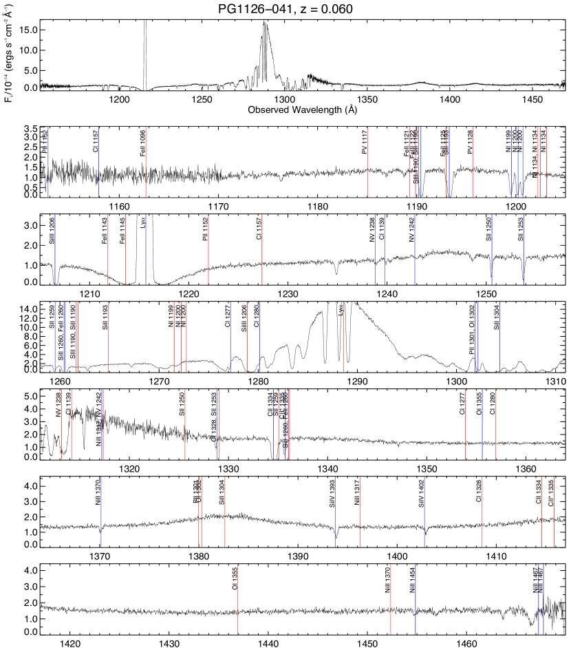
The starting point of the analysis is to identify the various emission and absorption lines produced by the quasars and their environments. Since our program is focused on QSO and ULIRG outflows, we only identify and measure absorption lines within 10,000 km s-1 of the QSO redshifts. We refer to these lines as “associated” absorbers. Identifications of the foreground “intervening” absorbers can be found in Tripp et al. (2008), Savage et al. (2014), and Danforth et al. (2016). We first compare each quasar spectrum against a list of common UV absorbers in quasar spectra (Prochaska et al., 2001, Figure 2). We list the quasar redshifts in Table 3. Most of these redshifts are derived from narrow optical emission lines ([O III], H) and may underestimate the true recession velocities since some fraction of the line emission may arise from the outflowing material itself (e.g. Rupke et al., 2017). See Teng et al. (2013) for a comparison of these measurements with the H I 21-cm emission and absorption line profiles.
Next, we fit the continuum and broad line emission (Ly, N V, and O VI) in three separate spectral windows around Ly, N V, and O VILy. In the two quasars in which we fit P V, this continuum region is also fit separately. Within each of these windows, we use a piecewise function of 1–4 segments in the majority of cases. In relatively featureless spectral regions, these segments are low-order polynomials. In more complex spectral regions we employ cubic B-splines. The B-splines are themselves piecewise polynomials, and we separate the spline knots by a typical interval of 3 Å. We invoke BSPLINE_ITERFIT from the SDSS IDLUTILS library to fit the B-splines.
In seven cases, the fits with piecewise functions are poorly constrained. For PG 1001054, PG 1004130, PG 1411442, and PG 1617175, PG2130099, and PG2214139 this is due to broad, deep absorption features over which it is difficult to fit polynomials or splines. For a seventh quasar—PG 1351640—the poor constraints are due to several narrow absorbers near the peak of Ly. In two of these cases, we instead use a Lorentzian profile to fit Ly. For the five others we use the BOSS template from Harris et al. (2016), scale it multiplicatively by a low-order power law, and add a linear pedestal.
After fitting the continuum, we normalize the data in each spectral window by dividing by this fit.
We characterize the doublet absorption features (N V 1238, 1243; O VI 1032, 1038; and P V 1117, 1128) in the quasar spectra using simple model fits. Our primary objectives are to estimate the overall equivalent widths and kinematics of the outflowing gas associated with these features (mass, momentum, and energy estimates are beyond the scope of the present paper, except for a few special cases discussed in Section 7.4). We are not aiming to derive precise column densities from the (often saturated) absorption line profiles, so the use of the precise COS line-spread function (LSF) is not required here (we return to this point at the end of this section). If the lines within these doublets were unblended, fits to the intensity profiles of the individual lines would thus be sufficient. However, the doublet lines are often strongly blended because of (1) strong blueshifts due to high outflow velocities and (2) broad line profiles due to multiple clouds along the line of sight and/or large linewidths. We thus adopt the doublet fitting procedure of Rupke et al. (2005), which is optimized for blended doublets. In this method, the total absorption profiles of a feature are fit as the product of multiple doublet components. Each component is a Gaussian in optical depth vs wavelength with a constant covering factor . Within each doublet the two lines have a constant ratio. This allows us to simultaneously fit and , which are otherwise degenerate in the fit of a single line. The free parameters in the fit to each doublet component are thus , peak , velocity width, and central wavelength. The determination of the number of components needed in the fit is subjective and non-linear it depends on the line complexity and data quality. The main goal here is to get a good fit to the absorption features to derive the equivalent widths and kinematics of the outflowing gas associated with these features. We do not attach a physical meaning to the individual components in the fit.
The general expression for the normalized intensity of a doublet component is
| (1) |
where is the line-of-sight covering factor (or the fraction of the background source producing the continuum that is covered by the absorbing gas; though scattering into the line of sight can also play a role) and and are the intrinsic optical depths of the lower- and higher-wavelength lines in the doublet (Rupke et al., 2005). The background light source is assumed to be spatially uniform. The covering factor is the same for both lines of the doublet. The peak (and total) optical depths of the resonant doublet lines in O VI, N V, and P V are related by a constant factor because of the 4-fold degeneracy in the upper state of the higher energy transition compared to the 2-fold degeneracy in the lower state. (The higher degeneracy is due in turn to its higher total angular momentum quantum number ). For more than one doublet component, we use the product of the intensities of the individual components, which is the partially-overlapping case of Rupke et al. (2005).
Because the doublet profile shape–i.e., relative depths of the two lines and trough shape–does not change significantly above optical depths of a few, we set a limit of . Out of 59 O VI components, 19 have , or 32%. For N V, 13 of 62 components have , or 21%.
The results from these fits are also used to calculate the total velocity-integrated equivalent widths of the absorbers in the object’s rest frame,
| (2) |
the weighted average outflow velocity,
| (3) |
and the weighted outflow velocity dispersion,
| (4) |
a measure of the second moment in velocity space of the absorbers in each quasar. These quantities are similar to those defined by Trump et al. (2006), but without the constraints on depth, width, or velocity. These constraints have little effect on the results for our sample, but we find it useful to include possibly inflowing absorbers. Note that , , and are not corrected for partial covering. To test the impact of this assumption on our results, we have recomputed them after changing the absorption lines so that they have instead of the measured , and then redid the regression analysis discussed in Sec. 5.2. Only very small changes of order 1% in the -values are observed if we correct for partial covering.
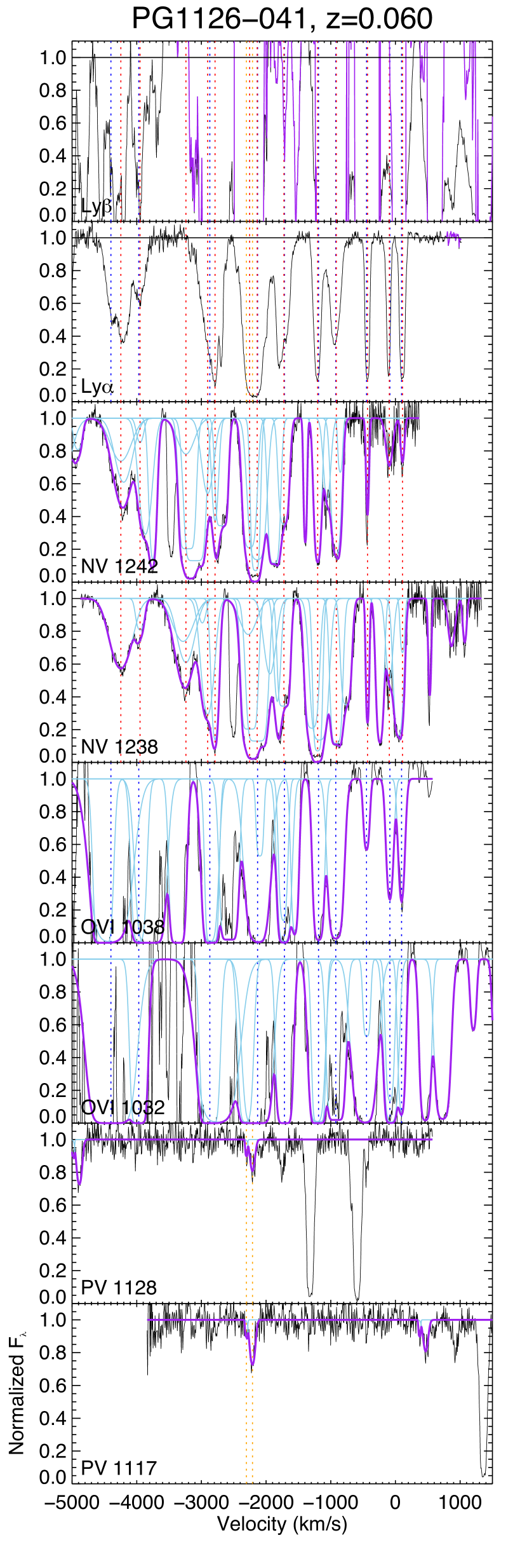
Figure 3 shows the fits to the spectrum presented in Figure 2. The fits to all of the features detected in the FUV spectra of the 33 quasars in our sample are presented in Appendix A, and the results derived from these fits are tabulated in Table 3.
We computed errors in best-fit parameters and derived model quantities by refitting the model spectrum 1000 times. In each case we added Gaussian-distributed random errors to each pixel in the model with equal to the measurement error. These formal errors are small due to the high S/N in our data. Errors due to continuum placement are likely to dominate the true error budget.
We also estimated upper limits to the doublet equivalent width in cases where we did not detect N V and/or O VI. To do so, we assumed an optically-thick ( or ), , km s-1 absorption line. We set the covering factor equal to half the root-mean-square deviation in the continuum within Å of the expected rest-frame location of each line in the doublet. (The factor-of-2 accounts for fitting 2 lines instead of 1.) We set the limit equal to the resulting model equivalent width.
The optical depths and covering factors derived from our fitting scheme are approximations. Though it is a physically-motivated way to decompose strongly-blended doublets, the method implicitly assumes that the velocity dependences of and can be described as the sum of discrete independent Gaussians. In reality, they are probably more complex functions of velocity (e.g. Arav et al., 2005, 2008). In several cases–the N V absorbers in PG 1001054, PG 1411442, PG 1617175, and PG2214139, and the O VI absorbers in PG 1001054 and PG 1004130–the fits include very broad components that cannot be distinguished from complexes of narrower lines given the data quality. In two O VI absorbers (PG 0923201 and PG 1309355), there are no data on the blue line because it is contaminated by geocoronal Ly, so any constraints on and come solely from line shape. Finally, in four O VI fits (PG 1001054, PG 1004130, PG 1126041, and PG 1617175), the Ly and O VI absorption lines blend together and cannot be easily separated in the fit. In three of these cases (all but PG 1001054), we simply fit the visible absorption as due solely to O VI at wavelengths in which there is at least some O VI absorption contributing to the spectrum. For the fourth case, we are able to roughly separate the lines by fitting only down to a specific wavelength. A detailed object-by-object discussion is given in Appendix A.
Despite these caveats, the fitting procedure is sufficient to meet our primary objectives of estimating the overall equivalent widths and kinematics of these features. The 3- detection limit on the doublet equivalent widths is typically 20 mÅ in our data although it varies from one spectrum to the other.
We have conducted detailed tests of the impact of the COS LSF on our measurements to verify that the use of the precise COS LSF is not required here. In one series of simulations, we created a series of fake, saturated Voigt line profiles with a median S/N of 5 per pixel and line widths ranging from = 10 km s-1 to 50 km s-1. We convolved the profiles with the LSF downloaded from the COS website. We find that the LSF causes a difference of up to only 10% on the line width and covering fraction measurements for lines with 20 km s-1 (the corresponding Doppler parameter of the Voigt profile is 28 km s-1), which is smaller than the values measured for nearly all of the absorbers detected in our objects (Table 3). We have also run a COS LSF analysis on a ULIRG with narrow N V absorption features, taken from the sample of Paper II. Using the method described here, we get a Doppler parameter of 78 km s-1 and covering fraction of 0.84, while the COS LSF gives 83 km s-1 and 0.82, respectively, confirming that the results for the relatively broad absorbers reported in the present paper are reliable.
| Name | Line | # comp. | |||
|---|---|---|---|---|---|
| Å | km s-1 | km s-1 | |||
| PG0007+106 | N V | 0.16 | |||
| PG0026+129 | N V | 0.09 | |||
| O VI | 0.12 | ||||
| PG0050+124 | N V | 0.88 | -1106.3 | 595.0 | 6 |
| PG0157+001 | N V | 0.13 | |||
| O VI | 0.09 | ||||
| PG0804+761 | N V | 0.02 | 591.0 | 12.3 | 1 |
| O VI | 0.18 | 571.0 | 27.8 | 1 | |
| PG0838+770 | N V | 0.12 | |||
| O VI | 0.06 | ||||
| PG0844+349 | N V | 0.73 | 151.4 | 31.8 | 2 |
| PG0923+201 | O VI | 4.48 | -3048.3 | 335.6 | 1 |
| PG0953+414 | O VI | 0.20 | -825.4 | 418.3 | 2 |
| PG1001+054 | N V | 6.07 | -5969.9 | 1326.5 | 4 |
| O VI | 11.61 | -5743.9 | 1092.4 | 6 | |
| PG1004+130 | O VI | 24.29 | -5335.7 | 2970.2 | 12 |
| PG1116+215 | O VI | 0.27 | -2271.6 | 908.7 | 2 |
| PG1126-041 | N V | 10.66 | -2085.5 | 1076.1 | 13 |
| O VI | 16.80 | -2559.2 | 1482.2 | 10 | |
| P V | 0.21 | -2234.2 | 48.2 | 2 | |
| PG1211+143 | N V | 0.05 | |||
| PG1226+023 | N V | 0.04 | |||
| O VI | 0.04 | ||||
| PG1229+204 | N V | 0.09 | |||
| Mrk 231 | N V | 0.18 | |||
| PG1302-102 | O VI | 0.05 | |||
| PG1307+085 | N V | 0.10 | |||
| O VI | 0.15 | -3406.2 | 66.8 | 2 | |
| PG1309+355 | O VI | 8.57 | -893.9 | 364.5 | 7 |
| PG1351+640 | N V | 4.36 | -1264.4 | 428.4 | 9 |
| PG1411+442 | N V | 10.30 | -1594.8 | 562.7 | 4 |
| P V | 0.83 | -1754.6 | 131.0 | 2 | |
| PG1435-067 | N V | 0.15 | |||
| O VI | 0.08 | ||||
| PG1440+356 | N V | 0.89 | -1478.4 | 775.3 | 3 |
| PG1448+273 | N V | 3.22 | -229.8 | 164.1 | 4 |
| PG1613+658 | N V | 0.14 | -3714.6 | 121.8 | 2 |
| O VI | 0.68 | -3691.1 | 126.6 | 2 | |
| PG1617+175 | N V | 3.00 | -3094.7 | 526.8 | 5 |
| O VI | 6.08 | -3323.7 | 920.2 | 8 | |
| P V | 0.06 | -3355.0 | 42.1 | 1 | |
| PG1626+554 | N V | 0.08 | |||
| O VI | 0.06 | ||||
| PG2130+099 | N V | 0.76 | -1312.3 | 540.3 | 3 |
| PG2214+139 | N V | 8.01 | -1461.1 | 681.7 | 5 |
| PG2233+134 | O VI | 0.17 | -211.2 | 17.3 | 1 |
| PG2349-014 | N V | 0.12 |
Note. — Column (1): Name of object. Column (2): N V means N V 1238, 1243, O VI means O VI 1032, 1038, and P V means P V 1117, 1128. N V or O VI is not listed when it lies outside of the spectral range of the data. Column (3): Velocity-integrated equivalent widths (eq. 2). Column (4): Average depth-weighted outflow velocity (eq. 3), which is a measure of the average velocity of the outflow systems in each object. Column (5): Average depth-weighted outflow velocity dispersion (eq. 4), which is a measure of the range in velocity of the outflow systems in each quasar. Column (6): Number of absorption components.
5.2 Regressions
To search for connections between outflow and quasar/host properties, we computed linear regressions between the properties in Tables 3 and 3. In most cases, we apply the Bayesian model in LINMIX_ERR (Kelly, 2007). We use the Metropolis-Hastings sampler and a single Gaussian to represent the distribution of quasar/host parameters (except for vs. AGN fraction, for which we used NGAUSS3). LINMIX_ERR permits censored y-values, which is the case for .
When we compute the regressions for the independent variable , however, the x-axis values are also censored. In this case we turn to the method of Isobe et al. (1986) for computing the Kendall tau correlation coefficient with censored data in both axes. We use the implementation of pymccorrelation (Privon et al., 2020), which in turn perturbs the data in Monte Carlo fashion to compute the errors in the correlation coefficient (Curran, 2014).
For both regression methods, we computed the significance of a correlation as the fraction of cross-correlation values () for a positive (negative) best-fit . For LINMIX_ERR, the values are draws from the posterior distribution, while for pymccorrelation they are results of the Monte Carlo perturbations.
We do not consider the N V and O VI points independent for the purposes of the regressions. Therefore, where both doublets are present in the data for a given quasar, we compute the average measurement (either detection or limit) from the two lines. If only one line is detected, we use that measurement rather than averaging a detection and a limit. Where multiple X-ray measurements exist for a quasar, we take the average. Errors in , , , and are unknown, so for the purposes of regression we fix the errors to 0.1 dex. For (UV), we ignore the negligible statistical measurement errors.
6 Results
The results from our spectral analysis of the HST spectra are summarized in Table 3. In this section, we investigate whether the presence or nature of quasar-driven outflows and starburst winds correlate with the properties of the quasars and host galaxies. The quantities that we consider in our correlation matrix are listed in Table 3 and defined in the notes to that table. The results from the statistical and regression analyses are summarized in Tables 4 and 5.
Note that we do not make a distinction between quasar-driven outflows and starburst-driven winds in this section, and we only consider absorption lines within 10,000 km s-1 of the QSO redshift (inclusion of lines at greater displacements leads to unacceptable contamination by intervening absorbers). A more comprehensive assessment of the detected outflows is conducted in Section 7, after we have considered the line profiles more fully, including signs of saturation and/or partial covering of the continuum source (Sec. 6.2) and the overall kinematics of the outflowing gas (Sec. 6.4). Similarly, the comparison of our results with those from previous studies is postponed until Section 7, once the results from our spectral analysis have been fully presented.
6.1 Rate of Incidence of Outflows
Figures 4 and 5 show the median velocities in the quasar rest frame of all of the detected N V and O VI absorption-line systems, sorted from top to bottom by decreasing redshift and bolometric luminosity, respectively. The first of these figures clearly illustrates the fact mentioned in Section 4 that our ability to detect the N V and O VI features is limited by the spectral coverage of the COS data to and , respectively (systems outside of the spectral range are indicated by an “x” in this figure and Fig. 5).
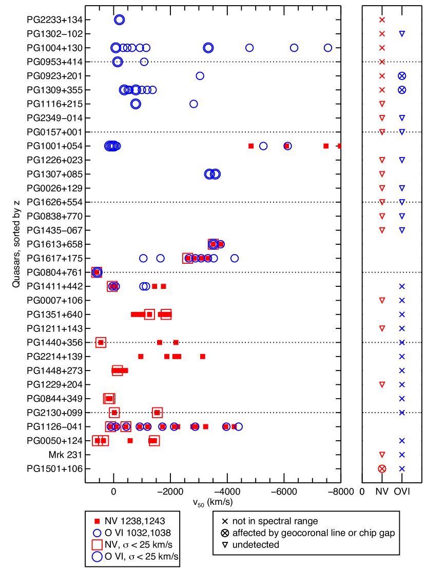
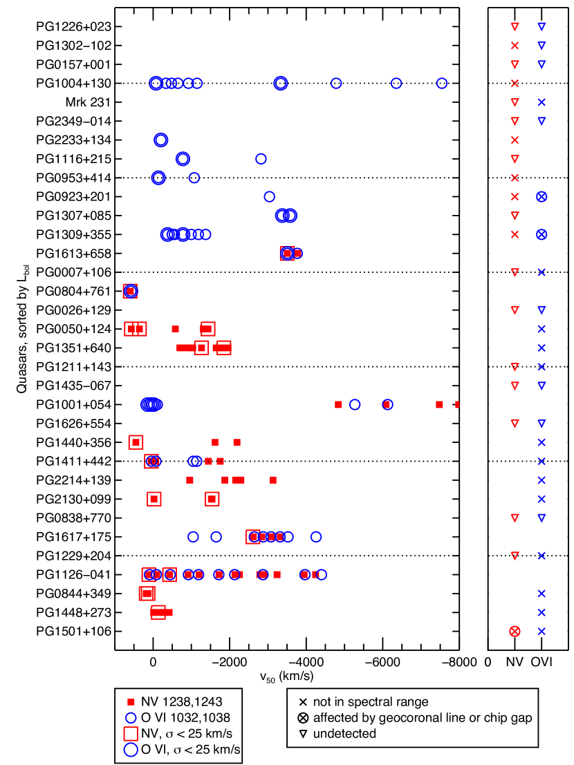
A cursory examination of Figures 4 and 5 shows that blueshifted N V or O VI absorption systems suggestive of outflows (with equivalent widths above our 3- detection limit of 20 mÅ) are detected in about 60% of the quasars in our sample, and there is no obvious trend in the rate of incidence with redshift or bolometric luminosity.
The results of a more quantitative analysis based on distributions (Cameron 2011) are listed in Table 4. The overall rate of incidence of N V or O VI absorbers is 61% with a 1- range of (52% 68%), once taking into account the spectral coverage of the data. This rate is virtually the same for N V and O VI. Among quasars with log 12.0, this rate is 61% with a 1- range of (49% 71%), while it is 60% (47% 71%) among the systems of lower luminosities. These rates are thus not significantly different from each other, and are similar to the rate of incidence of O VI outflows in local Seyfert 1 galaxies (Kriss, 2004a, b) as well as C IV (Crenshaw et al., 1999) or X-ray (Reynolds, 1997; George et al., 1998) absorption.
| Line | Detection | Total | Fraction (1- range) |
|---|---|---|---|
| (1) | (2) | (3) | (4) |
| All Quasars | |||
| N V | 13 | 27 | 0.48 (0.39 0.58) |
| O VI | 12 | 20 | 0.60 (0.49 0.70) |
| Both | 5 | 14 | 0.36 (0.25 0.50) |
| Any | 20 | 33 | 0.61 (0.52 0.68) |
| log 12.0 | |||
| N V | 4 | 12 | 0.33 (0.23 0.48) |
| O VI | 9 | 14 | 0.64 (0.50 0.75) |
| Both | 2 | 8 | 0.25 (0.16 0.44) |
| Any | 11 | 18 | 0.61 (0.49 0.71) |
| log 12.0 | |||
| N V | 9 | 15 | 0.60 (0.47 0.71) |
| O VI | 3 | 6 | 0.50 (0.32 0.68) |
| Both | 3 | 6 | 0.50 (0.32 0.68) |
| Any | 9 | 15 | 0.60 (0.47 0.71) |
| cm-2 | |||
| N V | 10 | 16 | 0.62 (0.50 0.73) |
| O VI | 8 | 8 | 1.00 (0.81 0.98) |
| Both | 3 | 5 | 0.60 (0.38 0.76) |
| Any | 15 | 19 | 0.79 (0.67 0.85) |
| cm-2 | |||
| N V | 2 | 10 | 0.20 (0.13 0.37) |
| O VI | 2 | 10 | 0.20 (0.13 0.37) |
| Both | 1 | 8 | 0.12 (0.08 0.32) |
| Any | 3 | 12 | 0.25 (0.17 0.41) |
| 1.6 | |||
| N V | 7 | 17 | 0.41 (0.31 0.53) |
| O VI | 6 | 12 | 0.50 (0.37 0.63) |
| Both | 2 | 9 | 0.22 (0.14 0.41) |
| Any | 11 | 20 | 0.55 (0.44 0.65) |
| 1.6 | |||
| N V | 6 | 9 | 0.67 (0.49 0.78) |
| O VI | 6 | 7 | 0.86 (0.64 0.91) |
| Both | 3 | 4 | 0.75 (0.48 0.85) |
| Any | 9 | 12 | 0.75 (0.59 0.83) |
Note. — Column (1): Feature(s) used in the statistical analysis. “Both” means both N V and O VI doublets and “Any” means either N V or O VI doublet or both; Column (2): Number of objects with detected outflows; Column (3): Number of objects in total with the appropriate redshift; Column (4): Fraction of objects with detected outflows. The two numbers in parentheses indicate the 1- range (68% probability) of the fraction of objects with detected outflows, computed from the distribution (Cameron, 2011).
| log() | 32 | 0.046 | -0.34 | |
| log[] | 32 | 0.140 | -0.22 | |
| AGN fraction | 32 | 0.094 | 0.78 | |
| log() | 32 | 0.054 | -0.33 | |
| log() | 32 | 0.289 | -0.33 | |
| Eddington Ratio | 32 | 0.168 | -0.42 | |
| 31 | 0.002 | -0.62 | ||
| log() | 32 | 0.067 | 0.37 | |
| log() | 30 | 0.094 | -0.29 | |
| log[] | 30 | 0.001 | 0.19 | |
| 30 | 0.143 | 0.25 | ||
| log[] | 26 | 0.005 | -0.54 | |
| log[] | 29 | 0.002 | -0.55 | |
| log[] | 26 | 0.072 | -0.33 | |
| log[] | 30 | 0.009 | -0.51 | |
| log[] | 26 | 0.051 | -0.38 | |
| log[] | 26 | 0.192 | 0.21 | |
| log[] | 26 | 0.211 | -0.20 | |
| log() | 20 | 0.138 | -0.27 | |
| log[] | 20 | 0.283 | -0.15 | |
| 20 | 0.103 | 0.31 | ||
| log() | 20 | 0.115 | 0.37 | |
| log() | 20 | 0.496 | 0.00 | |
| AGN fraction | 20 | 0.340 | 0.35 | |
| log() | 20 | 0.150 | -0.24 | |
| log() | 20 | 0.286 | -0.31 | |
| Eddington Ratio | 20 | 0.414 | 0.13 | |
| log[] | 18 | 0.034 | -0.15 | |
| 18 | 0.011 | 0.67 | ||
| log[] | 17 | 0.008 | 0.61 | |
| log[] | 17 | 0.016 | 0.57 | |
| log[] | 17 | 0.087 | 0.36 | |
| log[] | 18 | 0.264 | 0.17 | |
| log[] | 17 | 0.211 | 0.23 | |
| log[] | 17 | 0.006 | 0.69 | |
| log[] | 17 | 0.009 | 0.64 | |
| log() | 20 | 0.238 | 0.18 | |
| log[] | 20 | 0.425 | -0.04 | |
| 20 | 0.004 | -0.55 | ||
| log() | 20 | 0.305 | -0.16 | |
| log() | 20 | 0.433 | -0.04 | |
| AGN fraction | 20 | 0.389 | -0.13 | |
| log() | 20 | 0.247 | 0.17 | |
| log() | 20 | 0.301 | 0.29 | |
| Eddington Ratio | 20 | 0.374 | -0.18 | |
| log[] | 18 | 0.086 | 0.10 | |
| 18 | 0.048 | -0.46 | ||
| log[] | 17 | 0.016 | -0.56 | |
| log[] | 17 | 0.015 | -0.55 | |
| log[] | 17 | 0.066 | -0.40 | |
| log[] | 18 | 0.137 | -0.28 | |
| log[] | 17 | 0.120 | -0.32 | |
| log[] | 17 | 0.022 | -0.54 | |
| log[] | 17 | 0.008 | -0.61 |
Note. — Column (1): Dependent variable (absorption line property). Column (2): Independent variable (quasar/host property). Column (3): Number of points. Column (4): -value of null hypothesis (no correlation). Column (5): Correlation coefficient and 1 errors. Underlined entries under col. (2) indicate significant correlations with -values below 0.05.
We have also searched for trends between the rate of incidence of outflows and several other quantities. The detection rate of outflows (79%) among quasars that have strongly absorbed X-ray continua ( cm-2) is significantly higher than those that do not (25%) (Table 4). These rates differ at the 2- level (95.4%), where the ranges of the incidence rate are 56 92% for quasars with absorbed X-ray continua and 9 54% for the others. Using the scipy.stats implementation of the Fisher exact test, the null hypothesis that galaxies with strongly- and weakly-absorbed X-ray continua UV absorbers are equally likely to show N V or O VI absorbers is rejected at the 99.2% level. The rate of incidence of outflows among quasars with a steep X-ray to optical spectral index (; 75%) is also higher than those with a shallow index (55%), although the Fisher exact test shows that this difference is not significant (). A similar dependence on the X-ray properties of the quasars has been reported in several studies of higher luminosity quasars and lower luminosity Seyfert 1 galaxies using C IV 1548, 1550 as a tracer of warm ionized outflows. We return to this result in Sections 6.3 and 6.4, and 7.
6.2 Optical Depths and Covering Factors
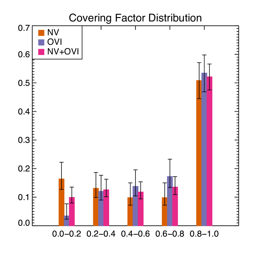
The distributions of the N V 1243 and O VI 1038 optical depths and covering factors derived from the individual components in the multi-component fits are presented as histograms in Figure 6.
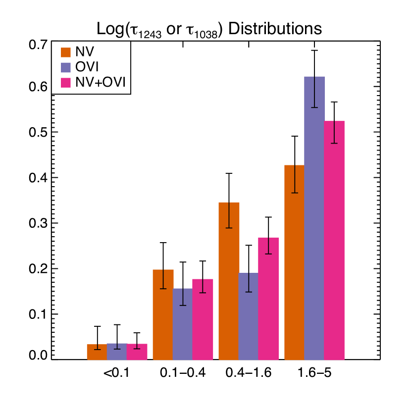
Again, we repeat that the optical depths and covering factors presented here are only approximations. Nevertheless, it is clear from the left panel in Figure 6 that a significant fraction of the absorbing systems are affected by saturation effects ( or 1), therefore making the equivalent widths of the N V and O VI features unreliable indicators of the total column densities of highly ionized gas in many of these cases.
The right panel of Figure 6 shows that the mode of the distribution of covering factors is consistent with unity, but 50% of the N V and O VI absorbers only partially cover the FUV quasar continuum emission (+ possibly the broad emission line region BELR; Fig. 6), consistent with small clouds located relatively near the quasars. As described at the end of Sec. 5.1, emission infill of the absorption profiles associated with the broad wings of the COS LSF is negligible and thus does not affect this conclusion. We return to this result in Section 7.1.
6.3 Outflow Equivalent Widths
The velocity-integrated equivalent widths (; eq. 2) of the outflow systems in each quasar are listed in Table 3. They span a broad range from 25 Å down to 20 mÅ, near our 3- detection limit.
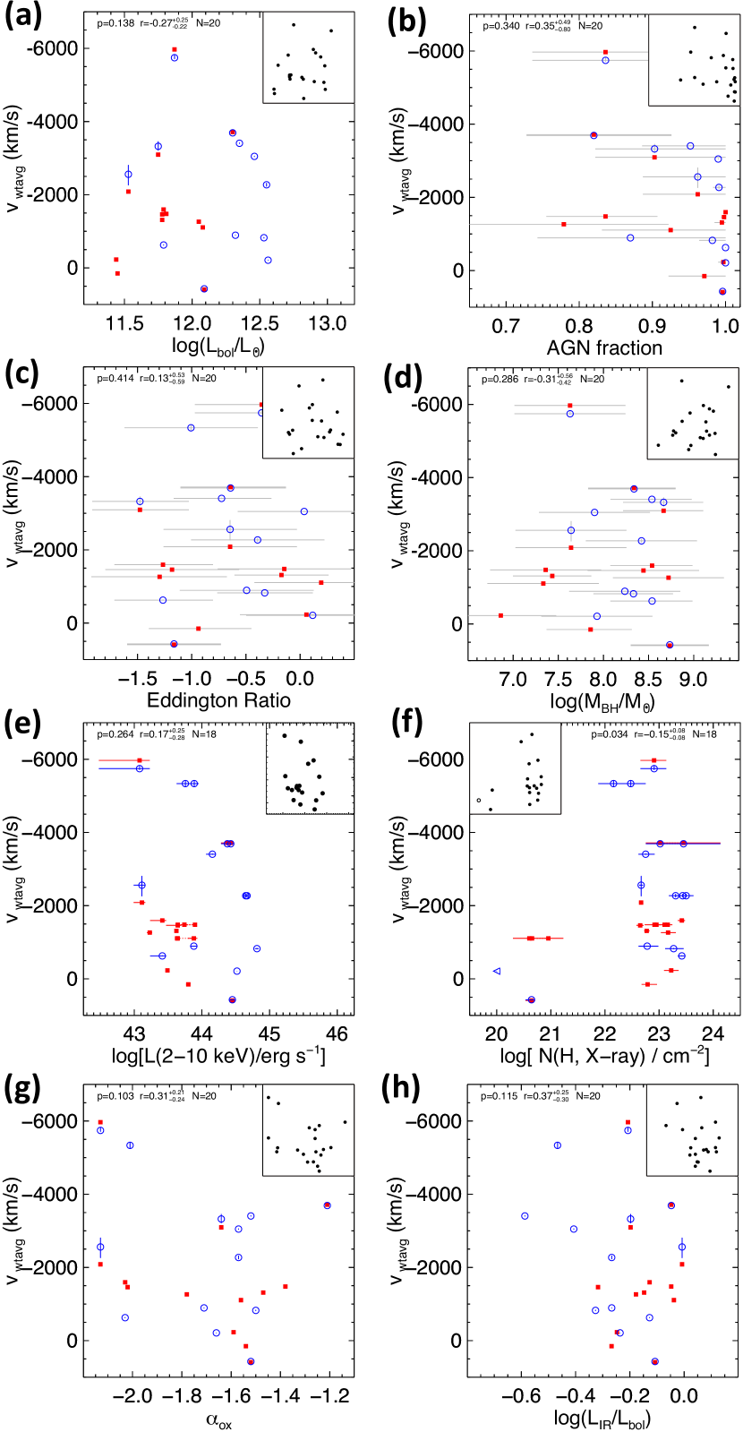
The equivalent widths of the outflows were compared against the properties of the quasars and host galaxies listed in Table 3. Some of the results are shown in Figure 7. By and large, we do not find any significant trends between and any of the quasar and host properties, except with some of the quantities that are derived from the X-ray data (Table 5). Taken at face value, this result is surprising since, for instance, it means that the equivalent width of the outflow is largely agnostic of the properties of the central engine over a range of 1.5 dex in power (FUV, bolometric, or quasar-only luminosity), 2.0 dex in Eddington ratio, and 2.5 dex in black hole mass. The lack of correlations with the properties of the hosts is less surprising since the quasar sample spans a relatively narrow range of values in these quantities so the lack of correlation with these quantities may be attributed to the lower dynamical range.

Examples of trends between and the X-ray properties of the quasars are shown in panels (e), (f), and (g) of Figure 7. In panel (e), the equivalent width of the outflow decreases with increasing HX luminosity. Panel (f) in this figure illustrates the dependence of the rate of incidence of these outflows on the X-ray column densities already pointed out in Section 6.1. The stronger highly ionized outflows with 1 Å are only present in quasars with X-ray column densities above 1022 cm-2. While it is a required condition for a strong outflow, it is not a sufficient condition since most quasars with these X-ray absorbing column densities show either weak outflows in the FUV ( 0.3 Å) or none at all. Panel (g) also shows a distinct trend for strong outflows with 1 Å among objects with . A similar trend is observed when normalizing the X-ray luminosities to the bolometric luminosities (not shown), but disappears when considering only the X-ray slope (e.g. the SX/HX ratio or index of the best-fit absorbed power-law distribution to the X-rays; not shown). Similar results have been found when considering C IV outflows (e.g. Brandt et al., 2000; Laor & Brandt, 2002; Baskin & Laor, 2005; Gibson et al., 2009a, b). We return to this issue in Section 7 below.
6.4 Outflow Kinematics
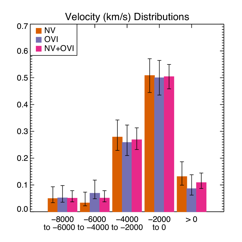
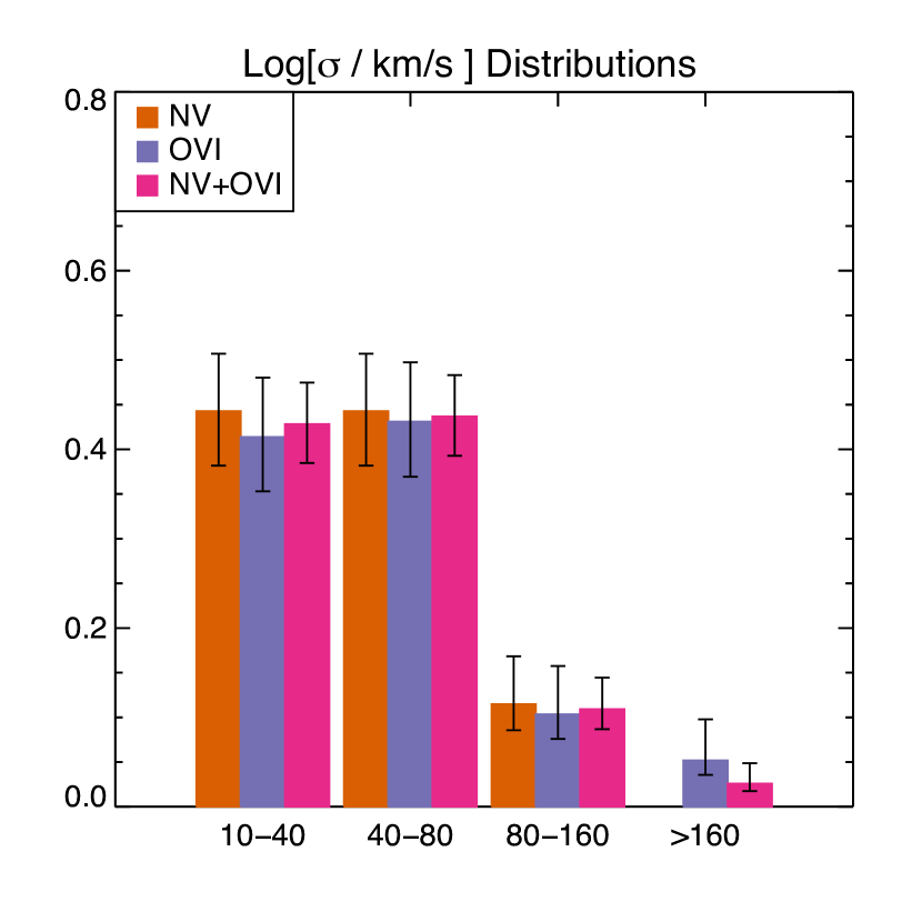
Figure 8 shows the distributions of the velocity centroids and dispersions () of the various individual components that were used to fit the N V and O VI absorbers in the quasar sample. About half of all of the individual components have blueshifted (outflow) velocities that lie between [2000, 0] km s-1 and have 1- widths less than 40 km s-1. In a blindly selected sample of O VI absorbers, Tripp et al. (2008) similarly found that the majority of associated absorbers are within 2000 km s-1 of the QSO redshift (see their Figure 15). Likewise, they found that the O VI line widths are 40 km s-1. Up to 10% of the individual components in the present survey have redshifted velocities of up to a few 100 km s-1; some of them may be attributed to uncertain or systematically blueshifted systemic velocities derived from the quasar emission lines (Sec. 5) rather than actual inflows.
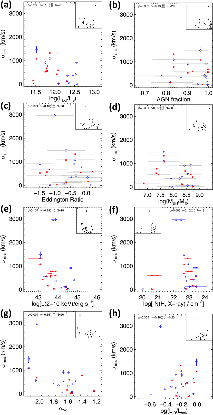
More physically meaningful kinematic quantities are the weighted average velocities and velocity dispersions of the outflow systems in each object (eqs. 3 and 4). Of the 20 detected absorbers in Table 3, 8 (3) have weighted average outflow velocities (velocity dispersion) in excess of 2000 (1000) km s-1.
We find in Table 5 that there is no distinct trend between the weighted outflow velocities and velocity dispersions and the quasar and host properties, except for the lack of outflows in X-ray unabsorbed quasars (Fig. 10), pointed out in Sec. 6.1, and the larger weighted outflow velocity dispersions among X-ray faint sources with . The lack of a correlation between outflow velocities and the quasar luminosities seems at odds with those from most previous C IV absorption-line studies (e.g. Perry & O’Dell, 1978; Brandt et al., 2000; Laor & Brandt, 2002; Ganguly et al., 2007; Ganguly & Brotherton, 2008; Gibson et al., 2009a, b; Zhang et al., 2014; Rankine et al., 2020) and other multi-wavelength analyses (e.g., references in Sec. 1 and Veilleux et al., 2020). We examine this issue in more detail in Section 7 below.
7 Discussion
7.1 Origins of the Absorption Features
The blueshifted N V and O VI absorption features reported in Section 6 may have several origins: quasar-driven outflows, starburst-driven winds, tidal debris from the galaxy mergers, and intervening CGM. Here we do not consider contamination of the quasar spectra by young stars since none of them show the obvious spectral signatures of young stars (e.g., narrow and shallow N V or O VI absorption troughs accompanied by redshifted emission). This is only an issue among starburst-ULIRGs (e.g. Martin et al., 2015).
Telltale signs that the detected lines are formed in a quasar-driven outflow include (1) line profiles that are blueshifted, broad, and smooth compared to the thermal line widths ( 10 20 km s-1 for highly ionized N4+, P4+, and O5+ ions at K), (2) line ratios within the multiplets N V 1238/1243, O VI 1032/1038, and P V 1117/1128 that imply partial covering of the quasar emission source, and (3) and large column densities in these high-ionization ions (Hamann et al., 1997b, a; Tripp et al., 2008; Hamann et al., 2019b). N V is typically very weak or absent in intervening systems (Werk et al., 2016). High N V/H I and O VI/H I are also much higher in associated absorbers than in intervening systems (e.g., Tripp et al., 2008).
Among the 20 quasars with N V or O VI absorption systems suggestive of outflows, 17 objects have absorption line profiles that meet the first of the above criteria (the only exceptions are PG 0804+761, PG 0844349, and PG 2233+134). Many of the quasars with blueshifted N V or O VI absorption lines show N V 1238/1243 and/or O VI 1032/1038 line ratios that also meet criteria #2 and #3 (Fig. 6). Mrk 231 does not formally meet these criteria (since it has no N V absorption line and O VI falls outside of the spectral range of the data), but it shows all of the characteristics of a FeLoBAL at visible and NUV wavelengths (and its Ly line emission is highly blueshifted; Veilleux et al., 2013b, 2016, and references therein), so we include it here among those with quasar-driven outflows. So, overall, at least 18 quasars in our sample have absorption features suggestive of quasar-driven outflows.
In 15 of the 20 absorber detections, the velocity widths, FWHM, are below the minimum of 2000 km s-1 generally used for BALs (Weymann et al., 1981, 1991; Hamann & Sabra, 2004; Gibson et al., 2009a, b), so they fall in the category of mini-BALs (500 FWHMrms 2000 km s-1) or NALs (FWHMrms 500 km s-1). Moreover, in many cases, the profiles are highly structured rather than smooth, and thus do not meet the “BAL-nicity” criterion to be true BALs.
The weak and narrow redshifted absorption features in PG 0804761 and PG 0844349 are good candidates for infalling tidal debris.
7.2 Location and Structure of the Mini-BALs
7.2.1 Depths of the Absorption Profiles
The depths of the mini-BALs may be used to put constraints on the location of the outflowing absorbers. The source of the FUV continuum in these quasars is presumed to be the accretion disk on scale of few 1015 cm ( 0.01 pc), where we used equation (6) in Hamann et al. (2019a) assuming an Eddington ratio . But it is clear from the spectra that in many cases (e.g., PG 1001054, 1004130, 1126041, 1309355, 1351640, 1411442, 2214139) the mini-BALs absorb not only the FUV continuum emission but also a significant fraction of the Ly, N V, and O VI line emission produced in the BELR. The gas producing the mini-BALs must therefore be located outside of the BELR on scales larger than
| (5) |
(e.g. Kaspi et al., 2005, 2007; Bentz et al., 2013). The radius of the outer boundary of the BELR, , is likely set by dust sublimation (Netzer & Laor, 1993; Baskin & Laor, 2018). For gas densities of 105 1010 cm-3, Baskin & Laor (2018) derive
| (6) | |||||
| (7) |
where graphite grains of size 0.05 m is assumed (Fig. 5 in Baskin & Laor, 2018). Note that these values are smaller than those in Barvainis (1987) and Veilleux et al. (2020), which are based on silicate grains and lower gas densities (thus lower evaporation temperatures).
More can be said about the structure of the absorbing gas from the fact that the N V and O VI absorption features are optically thick (; Fig. 6) but are not completely dark. The covering factors derived from the multi-component fits to the N V and O VI mini-BALs range from 0.1 to 1, a direct indication that the absorbing material is compact and spatially inhomoneneous. The often structured velocity profiles of the N V and O VI mini-BALs (N V in PG 1411442 is arguably the only exception) also suggest a high level of kinematic sub-structures in the outflows, different from the smooth BALs observed in high-luminosity quasars. These properties of the mini-BALs may indicate one of two things: (1) Our line of sight is not aligned along the direction of the outflowing stream of gas as in the case for the BALs (e.g. Murray et al., 1995; Elvis, 2000; Ganguly et al., 2001), but instead intercepts only a small fraction of this stream and results in a covering factor of the background emission that is highly dependent on the inhomogeneity of the outflowing gas. (2) Another equally plausible explanation is that (structured) mini-BALs form in more sparse outflows or (in the unified outflow model discussed for high-z quasars) in more sparse outflow regions, e.g., at higher latitudes above the disk.
7.2.2 Variability of the Absorption Profiles
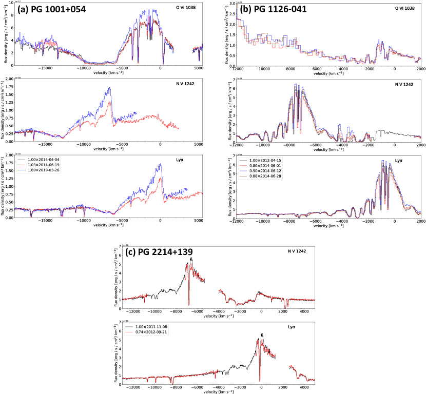
Additional constraints on the location and structure of the BALs and mini-BALS in our sample may be obtained from profile variability. There is a vast literature on this topic (e.g., Gibson et al., 2008; Hamann et al., 2008; Gibson et al., 2010; Capellupo et al., 2012; Filiz Ak et al., 2012, 2013; Grier et al., 2015; He et al., 2019; Yi et al., 2019, and references therein). In our sample, four of the mini-BALs (PG 1001054, PG 1126041, PG 1411442, and PG 2214139) have been observed at two different epochs or more, and can therefore be searched for mini-BAL profile variations. The emergence of a dense [log (cm-3) 7] new outflow absorption-line system in PG 1411442 was reported in Hamann et al. (2019b) and the detailed inferrence of a distance 0.4 pc from the quasar is not repeated here. We present the archival COS spectra for the other three objects in Figure 11, normalized to the same FUV continuum level to emphasize absorption profile variations.
In PG 1001054 (Fig. 11a), the dramatic (72%) decrease in the FUV continuum emission from June 2014 to March 2019 is accompanied by a strengthening of the broad Ly, N V, and O VI emission lines in terms of equivalent widths but no obvious change in the mini-BAL profiles. In PG 1126041 (Fig. 11b), the more modest (20%) decrease of the continuum emission from April 2012 to June 2014 are not accompanied by any obvious variations in the equivalent widths of any of the broad emission and absorption lines except for the most blueshifted N V absorption features below 3000 km s-1 which show variations on timescales perhaps as short as 12 days. The broad emission and absorption lines in PG 2214139 (Fig. 11c) show no variations between November 2011 and September 2021 despite a 26% increase in the strength of the FUV continuum emission.
The fast 12-day variability of the high-velocity N V mini-BAL in PG 1126041 may be interpreted in two different ways. One possibility is that transverse motions of the outflowing clouds across our line of sight to the continuum source and BELR are responsible for these changes (as in PG 1411442; Hamann et al., 2019b). A variant on this idea is that the changes in profiles are due instead to the dissolution and creation of the absorbing clouds/clumps in the outflow as they transit in front of the continuum source. In the other scenario, changes in the ionization structure of the absorbing clouds due to changes in the incident quasar flux cause the absorbing N V and O VI columns to vary and reproduce the observations. If this is the case, the variability timescale sets a constraint on the ionization or recombination timescale, which depends solely on the incident ionizing continuum and gas density ( 105 yrs/, where is the number density of the clouds in cm-3; e.g., He et al., 2019).
This last scenario predicts that changes in the FUV continuum of the quasar will produce changes in the mini-BAL. While changes are indeed observed in both the FUV continuum emission and high-velocity N V mini-BAL of PG 1126041, the amplitudes of these changes are not correlated. From 2012-04-15 to 2014-06-01, the continuum emission strengthened while the N V mini-BAL weakened. From 2014-06-01 to 2014-06-12, both the continuum emission and N V mini-BAL weakened. Finally, from 2014-06-12 to 2014-06-28, the continuum emission remained constant to within 1% but the N V mini-BAL strengthened slightly. This lack of a direct connection between variations in the continuum and the N V mini-BAL seems to disfavor the scenario where the mini-BAL variations are associated with changes in the ionization structure of the absorbing clouds, unless log (cm-3) 5-6 in which case and time delays associated with the finite recombination timescale could be at play (cf. Hamann et al., 2019b).
While more detailed modeling of the mini-BAL of PG 1126041 is beyond the scope of the present paper, the fact that the mini-BAL variations are only observed in N V and only at high velocities may be an optical depth effect: the cloud complex that produces the Ly and O VI mini-BALs and low-velocity N V mini-BAL may be so optically thick to be immune to variations in the ionizing continuum or tangential movement of the absorbing gas across the continuum source (we return to this topic in Sec. 7.4 below).
7.3 Driving Mechanisms of the Mini-BALs
As reviewed in, for instance, Veilleux et al. (2020), the absorbing clouds making up the mini-BALs may be material (1) entrained in a hot, fast-moving fluid, or (2) pushed outward by radiation or cosmic ray pressure, or (3) created in-situ from the hot wind material itself. In the first two scenarios, the equation of motion of the outflowing absorbers of mass that subtends a solid angle is
| (8) |
where is the galaxy mass enclosed within a radius and is a volume- and frequency-integrated optical depth that takes into account both single- and multiple-scattering processes in cases of highly optically thick clouds (Hopkins et al., 2014, 2020).333More explicitly, The value of therefore ranges from in the optically thin case to (1 + ) 1 in the infrared optically-thick limit (the effective infrared optical depth, , is also sometimes called the “boost factor”; Veilleux et al. (2020)). The terms on the right in Equation 8 are the forces due to the thermal, cosmic ray, and jet ram pressures, the radiation pressure, and gravity, respectively. Magneto-hydrodynamical effects are assumed to be negligible at the distances of these absorbing clouds. The quasars in our sample do not have powerful radio jets so the jet ram pressure term can safely be neglected. Similarly, the relatively modest radio luminosities of the mini-BAL quasars relative to their optical and bolometric luminosities (Column 6 in Table 3) suggest that cosmic-ray electrons do not play an important dynamical role in accelerating the BAL clouds. Indeed the fraction of BAL quasars seems to vary inversely with the radio loudness parameter, (Column 5 in Table 3; e.g., Becker et al., 2001; Shankar et al., 2008). Below, we consider the remaining thermal and radiation pressure terms separately. In reality, these pressure forces may act together to drive the mini-BAL outflows (see Sec. 7.4 for a closer look at the mini-BAL PG 1126041 in this context).
7.3.1 Thermal Wind and Blast Wave
For many years, ram-pressure acceleration of pre-existing clouds has been considered a serious contender to explain BALs in quasars given the need for a much hotter, rarefied medium to confine the clouds as they are being accelerated (e.g. Weymann et al., 1985). However, it is notoriouly difficult to accelerate dense gas clouds from rest up to the typical (mini-)BAL velocities by a warm, fast thermal wind without destroying them in the process through Rayleigh-Taylor fragmentation and shear-driven Kelvin-Helmholtz instabilities (e.g. Cooper et al., 2009; Scannapieco & Brüggen, 2015; Schneider & Robertson, 2015, 2017). Radiative cooling and magnetic fields may act to slow down cloud disruption (Marcolini et al., 2005; Cooper et al., 2009; Banda-Barragán et al., 2016, 2018, 2020; Grønnow et al., 2018). Radiative cooling of the warm mixed gas can not only prevent disruption, but it may cause the cloud to grow in mass (e.g., Gronke & Oh, 2018, 2020; Girichidis et al., 2021), although there are caveats (Schneider et al., 2020). An alternative scenario is that the BAL and mini-BAL clouds are created in-situ via thermal instabilities and condensation from the hot gas with a cooling time shorter than its dynamical time (Efstathiou, 2000; Silich et al., 2003). This is the idea behind the “blast wave” simulations of Richings & Faucher-Giguère (2018a, b); see also Weymann et al. (1985); Zubovas & King (2012, 2014); Faucher-Giguère & Quataert (2012); Nims et al. (2015).
In these simulations, a fast (presumably X-ray emitting) AGN wind with outward radial velocity of 30,000 km s-1 is injected in the central 1 pc and collides violently with the host ISM. The resulting shocked wind material reaches a very high temperature (1010 K; Nims et al., 2015) that does not efficienty cool, but instead propagates outward as an adiabatic (energy-driven) hot bubble. This expanding bubble sweeps up gas and drives an outer shock into the host ISM raising its temperature to a few 107 K (Nims et al., 2015). Radiative cooling of the shocked ISM eventually becomes important and the outflowing material reforms as cool neutral and molecular gas, but by that time, the outflowing material has acquired a significant fraction of the initial kinetic energy of the hot wind. These simulations predict that the cooling radius, i.e. the radius at which the gas cools to 104 K, increases from 100 pc to 1 kpc for AGN with luminosities from 1044 to 1047 erg s-1, respectively (Fig. 7 of Richings & Faucher-Giguère, 2018b). This cooling radius is also the expected location of the gas clouds producing the N V and O VI mini-BALs, as the cooling gas rapidly transitions from 107 K to 104 K. This large radius is well outside the lower limit on the distance of the mini-BAL from the quasars derived above so it is not inconsistent with our data. However, one should note that the inner X-ray wind in quasars is presumed to much smaller in reality than the value of 1 pc assumed in the simulations so the cooling radius may have to be scaled down accordingly. Moreover, these models do not address how the BELRs would be restored after the passage of the blast wave. Finally, the detailed analysis of the BAL in PG 1411442 firmly rule out (at least in that case) absorption at these large distances.
7.3.2 Radiative Acceleration
Although ram-pressure acceleration has been a serious contender, overall the favored explanation for the large velocities of the BALs and mini-BALs is that the gas absorbers have been accelerated by the radiation pressure forces associated with the intense radiation field that is emanating from the quasars (e.g., Arav et al., 1994; Giustini & Proga, 2019). Strong support for this scenario comes from the observed trends for the maximum velocity of the absorption to increase on average with increasing optical, UV, or bolometric luminosity and the Eddington ratio (e.g., Perry & O’Dell, 1978; Brandt et al., 2000; Laor & Brandt, 2002; Ganguly et al., 2007; Ganguly & Brotherton, 2008; Gibson et al., 2009b; Zhang et al., 2014). Note, however, that the overall correlations noted in these studies are often quite modest and sometimes only visible when considering the upper envelope of the velocity distribution and only when the sample of AGN span 2-3 orders of magnitude in luminosity (sometimes combining NALs, mini-BALs, and BALs together). While more recent studies (e.g., Rankine et al., 2020) have confirmed and indeed strengthened the existence of some of these correlations, all of the cited results relate to the C IV absorption, rather than the N V and O VI features. The statistics on N V and particularly O VI absorbers are much poorer.
Far Ultraviolet Spectroscopic Explorer (FUSE) observations of Seyfert galaxies of relatively low luminosities (1038 1042 erg s-1) show either no or very weak trends of increasing maximum velocities with increasing luminosities and no trend at all with the Eddington ratio (Kriss, 2004a, b; Dunn et al., 2008). O VI and N V BALs in high-redshift, high-luminosity quasars (Baskin et al., 2013; Hamann et al., 2019a) have maximum velocities that correlate with their C IV counterparts, but the range in AGN luminosity of their sample is too small to test the luminosity dependence of the maximum velocities. More fundamentally, there is also a trend between line widths and optical depth. The most extreme example of this trend is P V, which coexists with C IV having the same ionization requirements, but is always weaker and narrower than C IV (Hamann et al., 2019a). The reason is that P V traces only the highest column density regions with smaller covering fractions, while C IV can have significant absorption in more diffuse gas occupying a larger volume. This evidence for optical depth-dependent covering factors is a signature of inhomogeneous partial covering.
Overall, given the complex results from these previous studies, it is perhaps not surprising to find no significant correlations in our sample of QUEST quasars between (maximum) outflow velocities and the AGN luminosities (Sec. 6.4). Theoretically, the noise in the trends between the outflow kinematics and AGN luminosity is expected in the radiative acceleration scenario given projection effects that reduce the measured outflow velocities and variance in both the (minimum) launching radius (e.g. Laor & Brandt, 2002) and efficiency of radiative acceleration associated with the complex micro-physics of the photon interaction with the clouds - this complexity is hidden in the quantity in equation 8. A similar trend of increasing variance in the maximum velocity with increasing AGN luminosity is observed in the other cooler gas phases of AGN-driven outflows (e.g., Veilleux et al., 2020; Fluetsch et al., 2020).
Additional evidence that radiation pressure plays an important role in accelerating the absorbers in quasars comes from the significant dependence of the incidence rate, equivalent width, and weighted outflow velocity dispersion of the blueshifted absorbers on the X-ray properties of the quasars. This effect has been reported in numerous studies of nearby and distant AGN, based largely on C IV and Si IV (e.g., Laor & Brandt, 2002; Gibson et al., 2009b), and is also clearly present in our sample of quasars based on N V and O VI (Sec. 6.1, 6.3, and 6.4). More specifically, we find that mini-BALs and BALs are broader, stronger, and more common among X-ray faint quasars with steep optical-to-X-ray slopes 1.7 and hydrogen column densities in excess of 1022 cm-2 (Sec. 6). This result is expected in the context of radiative acceleration since the combined radiative force (“force multiplier”; Arav & Li, 1994) is greatly reduced when the gas is over-ionized by the hard far-UV/X-rays, becoming too transparent to be radiatively accelerated. This over-ionized “failed-wind” material may act as a radiative shield to produce the spectral softening needed for efficient radiative acceleration of the outflow material downstream (Murray et al., 1995; Proga & Kallman, 2004; Proga, 2007; Sim et al., 2010). However, the strong near-UV absorption lines near systemic velocity expected in this scenario are not observed (Hamann et al., 2013). Alternatively, the spectrum emerging from the accretion disk may be intrinsically softer/fainter in the hard far-UV/X-rays than commonly assumed (e.g. Laor & Davis, 2014). Weak-lined “wind-dominated” quasars, such as Mrk 231, PHL 1811 and its analogs, which are intrinsically faint and unabsorbed in the X-rays, may be naturally explained in this fashion (Richards et al., 2011; Wu et al., 2011; Luo et al., 2015; Veilleux et al., 2016). While a connection should exist between the X-ray warm absorbers and the UV absorption-line outflows, a direct one-to-one kinematic correspondence between the two classes of absorbers is often not seen because the gas in the warm absorbers is too highly ionized to produce measurable lines in the UV spectra (Kaspi et al., 2000, 2001; Gabel et al., 2003; Kraemer et al., 2001; Krongold et al., 2003; Arav et al., 2015; Laha et al., 2021, and references therein). We return to this point in Section 7.4 when discussing the mini-BAL in PG 1126041 (the case of PG 1211143 is briefly discussed in Appendix A).
Another observational characteristic of outflows that favors radiative acceleration is the phenomenon of line-locking observed in perhaps as many as 2/3 of all NAL and (mini-)BAL outflows (e.g., Hamann et al., 2011; Bowler et al., 2014; Lu & Lin, 2018; Mas-Ribas & Mauland, 2019, and references therein). This is observed in outflows where multiple absorbers are present but are separated by the exact same velocity separation as the doublet of C IV (499 km s-1), N V (962 km s-1), or O VI (1650 km s-1). Previous studies have shown that the probability of a line-locking signature accidentally occurring over a relatively small redshift path is negligible (e.g., Foltz et al., 1987; Srianand, 2000; Srianand et al., 2002; Ganguly et al., 2003; Benn et al., 2005). Radiative acceleration is a natural explanation for line-locking (e.g., Mushotzky et al., 1972; Scargle, 1973; Braun & Milgrom, 1989).
The best case for line-locking in our data is that of PG 1351640, where two deep absorption throughs are detected in Ly, extending over [2200, 1500] km s-1 and [1400, 600] km s-1, roughly separated by the velocity split of the N V doublet lines ( 900 1000 km s-1 ; Fig. 12). This results in a N V mini-BAL that looks like a “triplet” in this object. Another case of line-locking may be present in PG 1126041, where some of the deepest Ly throughs are separated by 900 1000 km s-1 (Fig. 3).
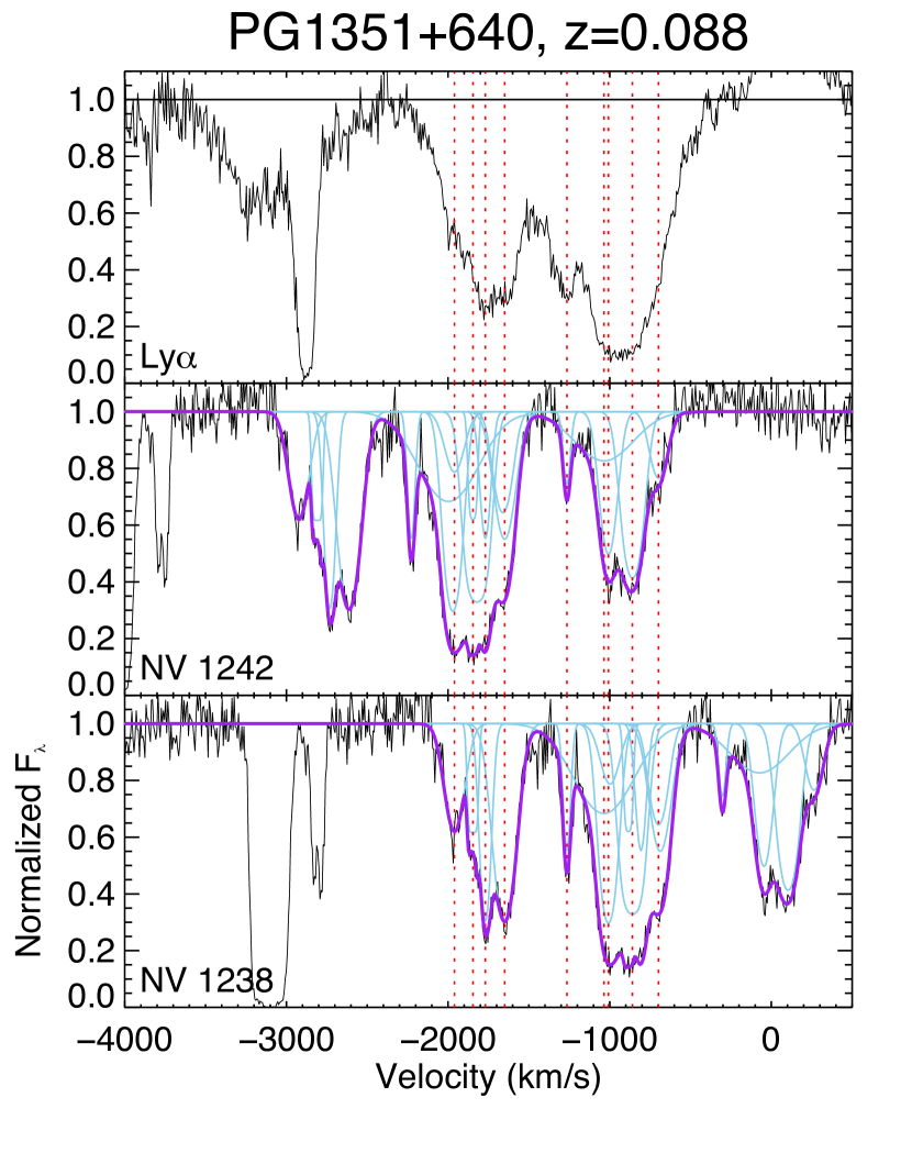
Note, finally, that radiation pressure on dust grains has also been invoked as an important contributor to the radiative acceleration given that (mini-)BAL QSOs, particularly LoBALs and FeLoBALs, have more reddened UV spectra than non-BAL QSOs (e.g., Allen et al., 2011; Hamann et al., 2019a, and references therein). This result has been interpreted to mean that BAL and mini-BAL clouds have large columns of ionized + neutral gas (log (cm-2) 23) and enough dust to provide extinction equivalent to at least 1-2 mag. in some cases (this is discussed in Sec. 7.4 in the context of PG 1126041, but see also the results on Mrk 231 and PG 1411442; Veilleux et al., 2016; Hamann et al., 2019b, respectively). Under these circumstances, the (mini-)BAL clouds may be subject to larger radiative forces than dustless clouds since the dust cross section, and thus in equation 8, in the UV optical is 1-2 orders of magnitude than the Thompson scattering cross section of electrons. Unfortunately, we do not have a reliable reddening indicator of the FUV continuum emission in our quasars, so we cannot directly compare our data with those of BAL and non-BAL QSOs. On the other hand, radiation that will be absorbed by the dust in the broad absorption line regions (BALRs) will be re-emitted in the infrared so our measurements of the infrared excess in our quasars may serve as a surrogate for the amount of dust in the BALRs. The lack of obvious correlation between BAL properties in our quasar sample and the mid-, far-, and total (1 1000 m) infrared excesses (e.g., Figs. 7 and 10) indicates one of two things: (1) radiative acceleration on dust is not important in the BALRs of these objects or (2) the various infrared excesses are dominated by dust emission from outside of the BALR, e.g. dust in the host galaxy itself.
7.4 P V Mini-BAL in PG 1126041 and Other Quasars
In this last section, we take a closer look at the mini-BAL system in PG 1126041. A mini-BAL extending from 1000 to 5000 km s-1 was first reported in the N V, C IV, and S IV absorption lines of this object by Wang & Wang (1999); Wang et al. (1999), based on the analysis of old low-resolution spectra obtained with IUE and the Goddard High-Resolution Spectrograph (GHRS) on HST. Variable and much faster (16,500 km s-1) X-ray absorption has also been detected in this object (Wang & Wang, 1999; Wang et al., 1999; Giustini et al., 2011). Interestingly, this object is among the least luminous AGN (log = 11.52) in our sample, intermediate between quasars and typical Seyfert 1 galaxies. Mini-BALs with outflow velocities of up to 5000 km s-1 and widths (FWHM) 1000 km s-1 are relatively rare in such low-luminosity systems (e.g., Kriss, 2004a, b; Dunn et al., 2008; Crenshaw & Kraemer, 2012). On the other hand, PG 1126041 is also the object in our sample with the steepest X-ray to optical index (, a virtual tie with PG 1001054, which also harbors a mini-BAL) and is among those with the largest infrared excess (Table 3), reinforcing the view expressed in Section 7.3.2 that X-ray absorbed or intrinsically weak quasars are more likely to host BALs and mini-BALs.
Apart from the line-locking signatures found in the N V mini-BAL of this object, which we argued in Sec. 7.3 favors radiative driving, the most remarkable aspect of this mini-BAL is the detection of a narrow P V 1117, 1128 cloud at a velocity of 2200 km s-1 (Fig. 3). Large ionized-gas column densities are needed to produce this feature given the low abundance of phosphorus relative to hydrogen (log(P/H)⊙ = 5.54; Lodders, 2003). The multi-component fit of each line in the P V doublet requires two components with nearly identifical median velocities (2196 and 2203 km s-1) but different velocity dispersions (24 and 74 km s-1), covering factors (0.37 and 0.10, respectively), and optical depths (0.7 and 2.6, respectively). The total equivalent width of this doublet is 0.3 Å.
Taken at face value, the results from the fits suggest that the P V lines are only moderately optically thick and therefore more reliable indicators of the total ionized column densities of this cloud than the highly saturated N V and O VI features. This is supported by the 2:1 intensity ratio of the P V lines. An optical depth of order unity in P V 1128 implies an ionized hydrogen column density log (cm-2) 22.3, assuming a solar P/H abundance ratio and ionization corrections based on detailed photoionization calculations for typical BALs and mini-BALs (ionization parameters log 0.5; Hamann, 1998; Leighly et al., 2011; Borguet et al., 2012, 2013; Baskin et al., 2014; Capellupo et al., 2017; Moravec et al., 2017; Hamann et al., 2019a, and references therein). This column density is remarkably consistent with the expectations from radiation pressure confined cloud models (Baskin et al., 2014).
This value of the total column density may be used to estimate the minimum kinematic energy of this outflowing cloud using (eq. 2 from Hamann et al., 2019a)
| (9) | |||||
where is an approximate global outflow covering factor based on the incidence of mini-BALs in the SDSS quasars (Trump et al., 2006; Knigge et al., 2008; Gibson et al., 2009b; Allen et al., 2011) and = 1 pc is a placeholder radial distance that we adopt for illustration purposes (it may underestimate the actual distance of the absorbers from the source; see Sec. 7.2 and Arav et al., 2020, and references therein). Following Hamann et al. (2019b), we estimate the time-averaged kinetic energy luminosity, , by dividing by a characteristic flow time, 450 yr. This yields erg s-1. In these units, = 1.3 1045 erg s-1 so 0.001. Taken at face value, this ratio is too small to significantly affect the evolution of the galaxy host (e.g., 0.005 is needed according to Hopkins & Elvis, 2010), unless (1) is severely underestimated or (2) the other clouds at lower and higher velocities involved in this mini-BAL contribute significantly to . This second possibility seems unlikely given the lack of P V detection in these clouds which suggests column densities log (cm-2) 22.
Next, we use the total column density of the P V cloud in PG 1126041 to estimate the time-averaged momentum outflow rate of this cloud, 1 1034 dynes, and compare this value with the radiation pressure, = 4 1034 dynes. Given that , radiation pressure can thus in principle accelerate this cloud, although a contribution from a thermally driven wind as detailed in Section 7.3.1 cannot be formally ruled out.
Finally, we apply Equation 9 and calculate for the other mini-BALs in our sample with solid and tentative P V detections. For PG 1411442, the only other mini-BAL in the sample with a definite P V detection, we get 0.01 and , for an outflow velocity of 1800 km s-1 (Table 3), a total column density log (cm-2) 23.4, and a BELR-like distance 0.4 pc from the central light source derived by Hamann et al. (2019b) using several absorption lines and detailed photoionization simulations. This BAL may thus be sufficient to impact the host galaxy evolution. P V is also tentatively detected in PG 1001054 and PG 1004130 at velocities of [4000, 6,000] km s-1 (Fig. 13). In both cases, the equivalent widths of P V 1117 and 1128 are very similar, implying saturation and log (cm-2) 22.3. These numbers yield outflows with kinetic-to-bolometric luminosity ratios that are higher than that of PG 1126041 but lower than that of PG 1411442, and thus marginally sufficient to impact the host galaxy evolution. Overall, the mini-BALs in the QUEST quasars are less powerful than the P V BALs detected in SDSS quasars (Moravec et al., 2017) but perhaps more common (4/33 10%) than at high luminosities/redshifts (detection rate of only 36% among the BAL quasars in the SDSS-III BOSS quasar catalog Capellupo et al., 2017).
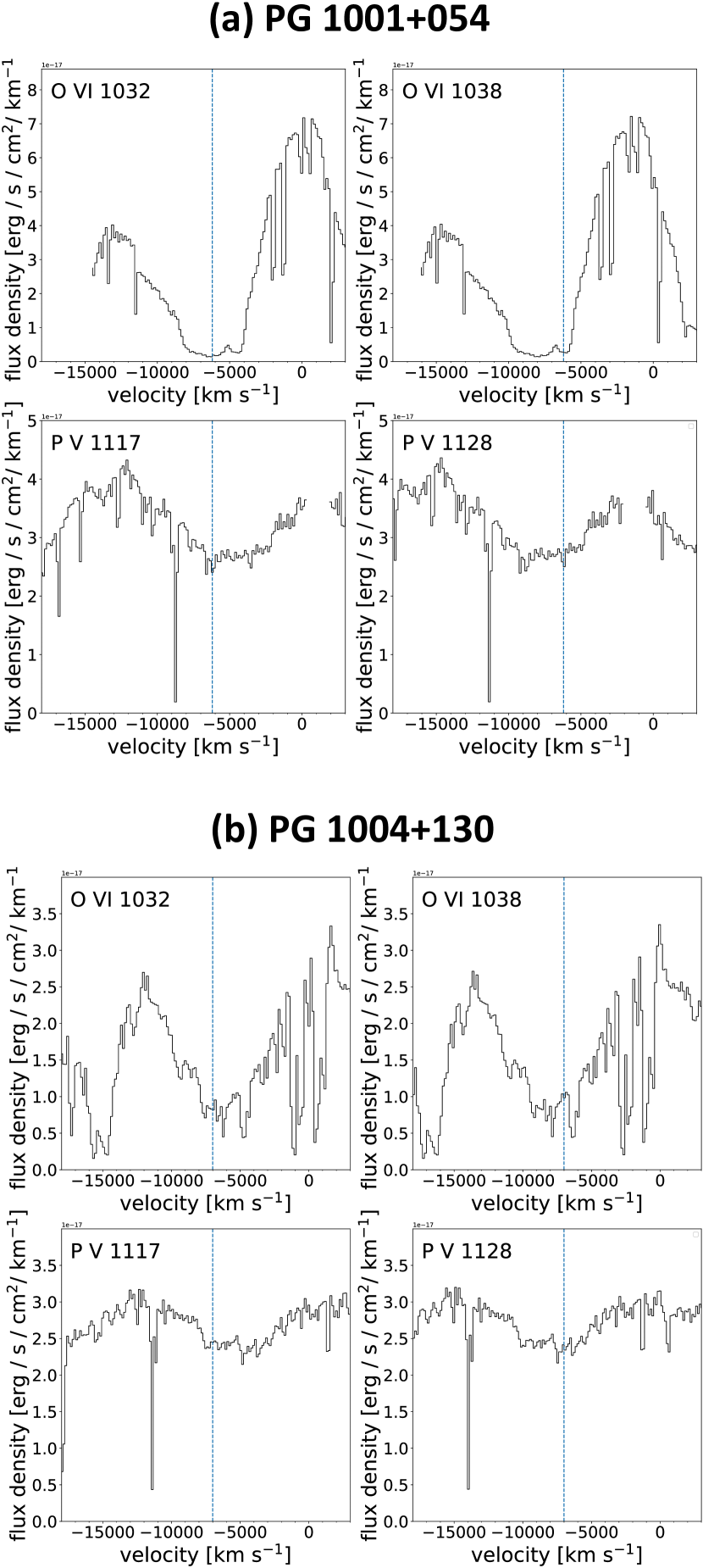
8 Summary
As part I of a HST FUV spectroscopic study of the QUEST (Quasar/ULIRG Evolutionary Study) sample of local quasars and ULIRGs, we have conducted a uniform analysis of the COS spectra of 33 Palomar-Green quasars. The main conclusions from our analysis are the following:
-
1.
Highly ionized outflows traced by blueshifted N V 1238, 1243 and O VI 1032, 1038 absorption lines with equivalent widths larger than 20 mÅ are present in about 60% of the QUEST quasars. This detection rate is similar to that of warm-ionized outflows traced by blueshifted C IV 1548, 1550 absorption lines in local Seyfert galaxies and more distant, higher luminosity quasars.
-
2.
The N V and O VI features in the QUEST quasars span a broad range of properties, both in terms of equivalent widths (from 20 mÅ to 25 Å) and kinematics (outflow velocities from a few 100 km s-1 up to 10,000 km s-1).
-
3.
The rate of incidence and equivalent widths of the highly ionized outflows are higher among X-ray weak sources with X-ray to optical spectral indices and X-ray column densities log (cm-2) 22. The weighted outflow velocity dispersions are highest in the X-ray weakest sources with X-ray to optical spectral indices . These results are qualitatively similar to AGN-driven warm ionized outflows traced by the C IV 1548, 1550 absorption lines. These results favor radiative acceleration of the absorbers, where the X-rays are either absorbed or intrinsically weak in the wind-dominated systems. Line-locking is detected in the Ly absorption throughs of one or two objects, providing additional evidence that radiation pressure plays an important role in accelerating these absorbers.
-
4.
There is no significant trend between the weighted average velocity of the highly ionized outflows and the properties of the quasars and host galaxies. This negative result is likely due in part to the fact that the range of properties of the QUEST quasar sample is narrow in comparison to those of other studies.
-
5.
Blueshifted P V broad absorption lines are clearly detected in PG 1126041 and PG 1411442 (previously reported in Hamann et al., 2019b), and also posssibly in PG 1001054 and PG 1004130. Using the results from the analysis of Hamann et al. (2019b), these features imply column densities of 1022.3 cm-2 or larger and time-averaged outflow kinetic power to bolometric luminosity ratios of 0.1% if a conservatively small radial distance of 1 pc from the P V absorbers is assumed.
Paper II of this series (Liu et al. 2021, in prep.) will present the results from our analysis of the COS spectra on the QUEST ULIRGs. These results will be combined with those from the present paper to provide a more complete picture of the gaseous environments of quasars and ULIRGs as a function of host galaxy properties and age across the merger sequence from ULIRGs to quasars.
Appendix A Detailed Results from the Spectral Analysis
Figures 14a14t present the fits to the detected N V, O VI, and P V absorption systems in our sample. The results from these fits are listed in Table 3 in the main body of the paper. Here we summarize the results from our spectral analysis for each object in the sample.
PG 0007106.—There are no associated N V absorbers in
this system, although two deep blueshifted and redshifted Ly absorption features are present at km s-1.
PG 0026129.—There are no associated N V or O VI
absorbers in this object.
PG 0050124 (I Zw 1).—N V and Ly absorbers are detected at
553, 1315, and 1467 km s-1 in this object.
Variable warm absorbers at 1870 and 2500 km s-1 have been
reported by Silva et al. (2018) in XMM-Newton RGS spectra obtained
in 2015.
PG 0157001 (Mrk 1014).—There are no associated N V or O VI
absorbers in this system.
PG 0804761.—This is a rare case for infall where
a strong redshifted absorption system at 600 km s-1 is observed in
Ly, and a corresponding weaker feature is also detected in N V and
O VI. The stronger features in the panel of Figure 14b
labeled O VI 1037 are Fe II features from the MW ISM.
PG 0838770.—A weak low- absorption
feature is seen in Ly but not N V or O VI.
PG 0844349.—A strong slightly redshifted
double-component absorption feature, likely associated with tidal
debris, is present at 140 km s-1 and 190 km s-1 in both Ly and N V, but the feature at 1288.9 Å has no corresponding
N V and is presumed to be Ly from intervening CGM.
PG 0923201.—A single broad absorber is observed at
3300 km s-1 in Ly, Ly, and O VI 1032 and 1038 although the glare
of the geocoronal Ly airglow truncates the blue wing of the O VI
1032 absorption line.
PG 0953414.—Two faint O VI features are detected at
140 and 1074 km s-1. The first feature is also
visible in Ly and Ly, but the more blueshifted feature
is not. The strong feature near 1271 Å cannot be fit with O VI and
thus is likely Ly from intervening CGM.
PG 1001054.—The multi-epoch COS spectra shown in
Figure 11 are co-added for this analysis
given the lack of variability in the absorption line profiles
(Sec. 7.2). This is a special case
because of the way the broad, high-velocity N V absorption absorbs the
Ly profile and the O VI absorption is deep, nearly dark, and highly
saturated. The three methods discussed in Section 5
were attempted to deal with the Ly + N V blend, and in the end
method #3 was used for the final fit: (1) The use of
polynomials/splines to fit the blue and red sides of Ly is
problematic because it does not appear to yield a symmetric Ly line
and seems to miss N V absorption that appears in Ly. (2) A
Lorentzian fit to Ly works reasonably well in that it yields a
symmetric line, but the line properties are highly unconstrained
(particularly in terms of height) and sensitive to the choice of which
continuum regions are fit. (3) After trying the QSO templates from
Vanden Berk et al. (2001),
Stevans et al. (2014),
and Harris et al. (2016), we settled on the last one. We scaled the
template using a constant offset, a constant multiplier, and a scaling
according to (arbitrary power ) to account for
differences between the spectral index and that of the template
(following Harris et al., 2016). We fit only the blue side of
Ly (and the far-red side) as well as some continuum regions in
between O VI and LyN V that are fairly line-free. This
underpredicts the strength of highly-ionized lines, but is the best
compromise solution. If the lines are fit as well, the blue side of
Ly is not properly fit. The resulting fit to N V seems to work
reasonably well, although the fit results are obviously illustrative
in terms of velocity space and certainly do not get the optical depth
correct. There seems to be a narrow Ly near 4000 km s-1 that is
barely detected in N V, but the fit has difficulties capturing it. The
broad, highly saturated, nearly dark O VI is fit over [6000, 4000]
km s-1 but not [8000, 6000] km s-1 to account for
Ly contamination. Broad blueshifted P V 1117, 1128 at
[6000, 4000] km s-1 is also tentatively detected in this object but
no attempt is made to fit this faint feature
(Fig. 13a).
PG 1004130.—This is another special case
(see Wills et al., 1999; Brandt et al., 2000, for some previous analyses). It is
difficult to fit the “continuum” shape and O VI profile
simultaneously. The present fit is the best available compromise. It
is clear that Ly / O VI are interacting with each other so the O VI
fit should be taken only as illustrative. There are higher-order Lyman
lines in the spectrum that are not considered. The Ly region
is shown but is not considered in the fits to O VI (the many narrow
features in the Ly region are Galactic ISM lines).
Blueshifted P V 1117 + 1128 at [6000, 4000] km s-1 is tentatively
detected but no attempt is made to fit this faint feature
(Fig. 13b).
PG 1116215.—There are several narrow absorption
features blueward of Ly, O VI, and Ly in this system, but only
two of them are paired in O VI 1032 and 1038,
corresponding to 771 and 2825 km s-1. Presumably, the orphan
features are intervening Ly absorbers. Savage et al. (2014) also
report an O VI system at 1175 and 1181 Å, but it is not shown here
as it is very narrow and very high velocity, and is intervening CGM
(there are nearby galaxies at the same redshift Tripp et al., 1998).
PG 1126041.—Several separate COS/G130M spectra exist
for this object (Table 2). Our analysis uses the
co-added spectrum. Broad blueshifted absorption features are clearly
detected in Ly, N V, and O VI (Fig. 3).
A narrow P V feature is observed at 2200 km s-1, indicative of large
ionized column densities. This P V detection is discussed in more
detail in Section 7.4. 2014 and 2015
COS/G160M spectra centered around 1450 Å show strong C IV
1548, 1550 absorption throughs similar to those of N V
and O VI, but only weak and narrow blueshifted S IV
1392, 1402 absorption features with
500 km s-1; the analysis of these features is beyond the scope of
the present study.
PG 1211143.—There are no associated N V absorption
systems in this object. A broad absorption feature at the observed
wavelength of 1240 Å has been interpreted by Kriss et al. (2018) as a
highly blueshifted (16,980 km s-1) and broad (FWHM 1080 km s-1)
Ly absorption from a fast wind. It may correspond to one of the
ultra-fast outflowing systems detected in the X-rays (Danehkar et al., 2018, and
references therein). However, since it is not
detected in N V
it is not included in the statistical analysis of Section
6.
PG 1226023 (3C 273).—The FUV spectrum of 3C 273 has been used
extensively to study the low- IGM
(e.g., Tripp et al., 2008; Savage et al., 2014). There are no associated N V or
O VI absorption systems in this object.
PG 1229204.—There are no associated N V absorption
systems in this object. The many unidentified features shortward of
Ly in the quasar rest-frame (e.g., 1289.5, 1282, 1223.2, 1220.4
Å) may be Ly from intervening CGM.
Mrk 231.—The 2011 COS/G130M spectrum of this object was
presented in Veilleux et al. (2013a),
while the 2014 COS/G140L and G230L spectra
were presented in Veilleux et al. (2016). The COS/G130M spectrum shows
Ly emission that is broad ( 10,000 km s-1) and highly blueshifted
(centroid at 3500 km s-1). In contrast, blueshifted absorption
features are only present above 2200 Å. These results have
been discussed in details in Veilleux et al. (2016), and this discussion
is not repeated here. This outflow is considered a non-detection in
our analysis in Section 6 since it has no N V
absorption systems, but has all of the characteristics of a FeLoBAL at
visible and NUV wavelengths and is considered as such in our
discussion (Sec. 7).
PG 1302102.—There are no associated O VI absorbing
systems in this object, but several intervening Ly and
metal-line systems have been reported by Cooksey et al. (2008).
PG 1307085.—The weak O VI absorber at 3400
km s-1 is also detected in Ly and Ly. The other feature
at 3600 km s-1 is seen only in Ly and Ly and
is presumed to be from intervening CGM.
PG 1309355.—A broad absorption feature is visible in
Ly, extending blueward to 1600 km s-1. This feature is also
detected in both O VI lines, but is truncated by the gap associated
with the strong geocoronal Ly emission. Strong absorption features
are detected coincident with P V 1117 and 1128 near systemic velocity,
but given their equivalent widths they are likely of Galactic origin
(e.g. C II 1334).
PG 1351640.—Two deep broad absorption throughs are
detected in N V and Ly of this object, extending over [2200,
1500] km s-1 and [1400, 600] km s-1. They are roughly
separated by the velocity separation of the N V doublet lines,
resulting in a N V “triplet”, so this is a good case for line
locking (Sec. 7.3.2). The template fit to
the Ly line emission works well in the very narrow region in which
it is used, but mostly because it gets the smooth profile in this
region better than a spline+polynomial fit. The central peak is
steeper than the template, and it is possible that the bluest
absorption region in Ly at [3500, 2500] km s-1 is caused by a
weak peak rather than a true absorption, since it does not line up
with anything in N V. The N V template fit, again over this limited
range, is quite good and more trustworthy over a wider wavelength
range. It is actually quite comparable to the spline fit. It does not
get the steep central peak in Ly on the red side.
PG 1411442.—This object has been the subject of a
detailed analysis by Hamann et al. (2019b). A deep broad absorption
through that extends over [2800, 900] km s-1 is present in N V
and Ly. Strong P V absorption is also detected over [2200, 1400]
km s-1 in this object. The absorption profiles presented here should be
taken only as illustrative. They are produced using a simple
spline/polynomical fit to the line emission + continuum. The quasar
template is much too broad to match the observed emission line
profiles of Ly and N V.
PG 1435067.—There are no associated N V or O VI
absorption systems in this object, but a faint Ly absorber appears
to be present at 1369.3 Å or 700 km s-1. The other
bluer narrow absorption features are likely Ly absorption from the
intervening CGM.
PG 1440356.—Two blueshifted N V absorbers are
observed at 2190 and 1610 km s-1, and a fainter redshifted one
at 460 km s-1 is also detected in both lines of the doublet. Note
that the strongest of the blueshifted N V systems does not have a
good match in velocity space with Ly. The strong line near 1334
Å is produced in the Galactic ISM, while the strong line blueward
of Ly is presumably produced by intervening CGM. The
Ly line at 200 km s-1 may be systemic within the uncertainties
on the redshift or a signature of inflow.
PG 1448273.—A broad (FWZI 700 km s-1)
multi-component absorption feature is detected in both N V and
Ly. The narrow Ly feature at 2700 km s-1 is
likely produced by intervening CGM, while the deep saturated feature
at 1280 Å is C I from Galactic ISM.
PG 1501106.—Three strong absorption features are
seen blueward of Ly at 1253.0, 1255.8, and 1257.2 Å,
corresponding to 1500, 800, and 500 km s-1, respectively
(the absorption near 0 km s-1 is at least partly due to S II from
Galactic ISM). Despite the chip gap at the position of the N V
doublet, the present data allow us to rule out the presence of a N V
1238 counterpart to the most highly blueshifted of these
Ly features since it would lie near 1276.5 Å and is not
present in the data.
PG 1613658.—Two weak narrow absorption features are
detected at 3503 and 3764 km s-1 in N V, O VI, and Ly. The
other features around N V are of Galactic ISM origin, while those in
O VI and Ly are likely due to intervening CGM.
PG 1617175.—A broad (1000 km s-1) blueshifted
absorption feature centered around 3000 km s-1 is detected in
N V, O VI, and Ly. Three narrow absorbers at 3300, 1630, and
1040 km s-1 are also detected in O VI and Ly but are very weak or
absent in N V.
PG 1626554.—The two distinct blueshifted Ly absorption features at 1378.8 Å and 1374.7 Å, corresponding to
740 and 570 km s-1 in the quasar rest frame, are also detected in
Ly but not in N V. A faint depression at 1166.9 Å may be the
570 km s-1 counterpart of O VI 1032 but it is not detected in the
fainter O VI 1038. This feature was judged too uncertain to be
a detection in our analysis.
PG 2130099.—Two deep and narrow absorption features
at 1500 and 0 km s-1 are detected in N V and Ly of
this object.
PG 2214139.—Our analysis is based on the co-added
spectrum of this object given the lack of variability in the
absorption lines between 2011 and 2012
(Fig. 11). This object shows complex N V
troughs that extend from 3400 to 400 km s-1 and are
loosely matched to the complex absorption feature at Ly, except
for the sharp Ly absorption feature near 100 km s-1, which is
not detected in N V.
PG 2233134.—This object shows a faint and narrow
absorber at 200 km s-1 in O VI and Ly. The Ly absorber at 1300 km s-1 also seems to have a weak O VI
counterpart but the fit is inconclusive and is therefore not included
in the statistics for this object. The other stronger lines in this
spectral region do not match Galactic ISM features so they are likely
produced by intervening CGM.
PG 2349014.—There are no N V or O V 1032
absorbers in this object (O VI 1038 is lost in the glare of
geocoronal Ly).
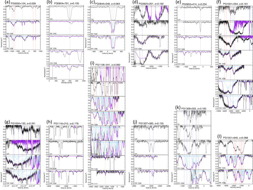
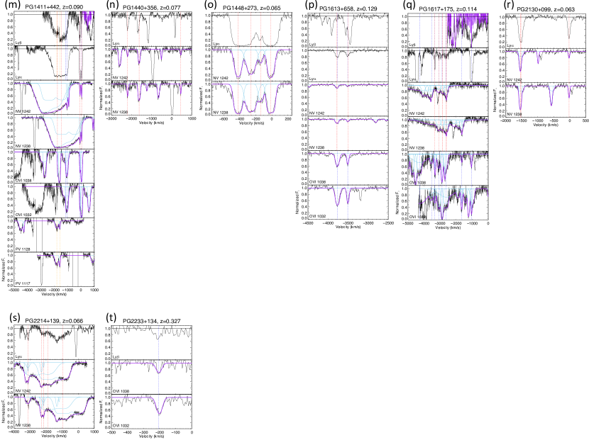
References
- Allen et al. (2011) Allen, J. T., Hewett, P. C., Maddox, N., Richards, G. T., & Belokurov, V. 2011, MNRAS, 410, 860, doi: 10.1111/j.1365-2966.2010.17489.x
- Arav et al. (2005) Arav, N., Kaastra, J., Kriss, G. A., et al. 2005, ApJ, 620, 665, doi: 10.1086/425560
- Arav & Li (1994) Arav, N., & Li, Z.-Y. 1994, ApJ, 427, 700, doi: 10.1086/174177
- Arav et al. (1994) Arav, N., Li, Z.-Y., & Begelman, M. C. 1994, ApJ, 432, 62, doi: 10.1086/174549
- Arav et al. (2008) Arav, N., Moe, M., Costantini, E., et al. 2008, ApJ, 681, 954, doi: 10.1086/588651
- Arav et al. (2020) Arav, N., Xu, X., Miller, T., Kriss, G. A., & Plesha, R. 2020, ApJS, 247, 37, doi: 10.3847/1538-4365/ab66af
- Arav et al. (2015) Arav, N., Chamberlain, C., Kriss, G. A., et al. 2015, A&A, 577, A37, doi: 10.1051/0004-6361/201425302
- Banda-Barragán et al. (2020) Banda-Barragán, W. E., Brüggen, M., Federrath, C., et al. 2020, MNRAS, 499, 2173, doi: 10.1093/mnras/staa2904
- Banda-Barragán et al. (2018) Banda-Barragán, W. E., Federrath, C., Crocker, R. M., & Bicknell, G. V. 2018, MNRAS, 473, 3454, doi: 10.1093/mnras/stx2541
- Banda-Barragán et al. (2016) Banda-Barragán, W. E., Parkin, E. R., Federrath, C., Crocker, R. M., & Bicknell, G. V. 2016, MNRAS, 455, 1309, doi: 10.1093/mnras/stv2405
- Barvainis (1987) Barvainis, R. 1987, ApJ, 320, 537, doi: 10.1086/165571
- Baskin & Laor (2005) Baskin, A., & Laor, A. 2005, MNRAS, 356, 1029, doi: 10.1111/j.1365-2966.2004.08525.x
- Baskin & Laor (2018) —. 2018, MNRAS, 474, 1970, doi: 10.1093/mnras/stx2850
- Baskin et al. (2013) Baskin, A., Laor, A., & Hamann, F. 2013, MNRAS, 432, 1525, doi: 10.1093/mnras/stt582
- Baskin et al. (2014) Baskin, A., Laor, A., & Stern, J. 2014, MNRAS, 445, 3025, doi: 10.1093/mnras/stu1732
- Becker et al. (2001) Becker, R. H., White, R. L., Gregg, M. D., et al. 2001, ApJS, 135, 227, doi: 10.1086/321798
- Benn et al. (2005) Benn, C. R., Carballo, R., Holt, J., et al. 2005, MNRAS, 360, 1455, doi: 10.1111/j.1365-2966.2005.09143.x
- Bentz & Katz (2015) Bentz, M. C., & Katz, S. 2015, PASP, 127, 67, doi: 10.1086/679601
- Bentz et al. (2013) Bentz, M. C., Denney, K. D., Grier, C. J., et al. 2013, ApJ, 767, 149, doi: 10.1088/0004-637X/767/2/149
- Borguet et al. (2013) Borguet, B. C. J., Arav, N., Edmonds, D., Chamberlain, C., & Benn, C. 2013, ApJ, 762, 49, doi: 10.1088/0004-637X/762/1/49
- Borguet et al. (2012) Borguet, B. C. J., Edmonds, D., Arav, N., Benn, C., & Chamberlain, C. 2012, ApJ, 758, 69, doi: 10.1088/0004-637X/758/1/69
- Boroson & Green (1992) Boroson, T. A., & Green, R. F. 1992, ApJS, 80, 109, doi: 10.1086/191661
- Bowler et al. (2014) Bowler, R. A. A., Hewett, P. C., Allen, J. T., & Ferland, G. J. 2014, MNRAS, 445, 359, doi: 10.1093/mnras/stu1730
- Brandt et al. (2000) Brandt, W. N., Laor, A., & Wills, B. J. 2000, ApJ, 528, 637, doi: 10.1086/308207
- Braun & Milgrom (1989) Braun, E., & Milgrom, M. 1989, ApJ, 342, 100, doi: 10.1086/167578
- Cameron (2011) Cameron, E. 2011, PASA, 28, 128, doi: 10.1071/AS10046
- Capellupo et al. (2012) Capellupo, D. M., Hamann, F., Shields, J. C., Rodríguez Hidalgo, P., & Barlow, T. A. 2012, MNRAS, 422, 3249, doi: 10.1111/j.1365-2966.2012.20846.x
- Capellupo et al. (2017) Capellupo, D. M., Hamann, F., Herbst, H., et al. 2017, MNRAS, 469, 323, doi: 10.1093/mnras/stx870
- Carilli et al. (1998) Carilli, C. L., Wrobel, J. M., & Ulvestad, J. S. 1998, AJ, 115, 928, doi: 10.1086/300253
- Cicone et al. (2014) Cicone, C., Maiolino, R., Sturm, E., et al. 2014, A&A, 562, A21, doi: 10.1051/0004-6361/201322464
- Cooksey et al. (2008) Cooksey, K. L., Prochaska, J. X., Chen, H.-W., Mulchaey, J. S., & Weiner, B. J. 2008, ApJ, 676, 262, doi: 10.1086/528704
- Cooper et al. (2009) Cooper, J. L., Bicknell, G. V., Sutherland, R. S., & Bland-Hawthorn, J. 2009, ApJ, 703, 330, doi: 10.1088/0004-637X/703/1/330
- Crenshaw & Kraemer (2012) Crenshaw, D. M., & Kraemer, S. B. 2012, ApJ, 753, 75, doi: 10.1088/0004-637X/753/1/75
- Crenshaw et al. (1999) Crenshaw, D. M., Kraemer, S. B., Boggess, A., et al. 1999, ApJ, 516, 750, doi: 10.1086/307144
- Curran (2014) Curran, P. A. 2014, arXiv e-prints, arXiv:1411.3816. https://arxiv.org/abs/1411.3816
- Danehkar et al. (2018) Danehkar, A., Nowak, M. A., Lee, J. C., et al. 2018, ApJ, 853, 165, doi: 10.3847/1538-4357/aaa427
- Danforth et al. (2010) Danforth, C. W., Keeney, B. A., Stocke, J. T., Shull, J. M., & Yao, Y. 2010, ApJ, 720, 976, doi: 10.1088/0004-637X/720/1/976
- Danforth et al. (2016) Danforth, C. W., Keeney, B. A., Tilton, E. M., et al. 2016, ApJ, 817, 111, doi: 10.3847/0004-637X/817/2/111
- Dasyra et al. (2007) Dasyra, K. M., Tacconi, L. J., Davies, R. I., et al. 2007, ApJ, 657, 102, doi: 10.1086/510552
- de Vaucouleurs et al. (1991) de Vaucouleurs, G., de Vaucouleurs, A., Corwin, Herold G., J., et al. 1991, Third Reference Catalogue of Bright Galaxies
- Dunn et al. (2008) Dunn, J. P., Crenshaw, D. M., Kraemer, S. B., & Trippe, M. L. 2008, AJ, 136, 1201, doi: 10.1088/0004-6256/136/3/1201
- Efstathiou (2000) Efstathiou, G. 2000, MNRAS, 317, 697, doi: 10.1046/j.1365-8711.2000.03665.x
- Elvis (2000) Elvis, M. 2000, ApJ, 545, 63, doi: 10.1086/317778
- Evans et al. (2006) Evans, A. S., Solomon, P. M., Tacconi, L. J., Vavilkin, T., & Downes, D. 2006, AJ, 132, 2398, doi: 10.1086/508416
- Faucher-Giguère & Quataert (2012) Faucher-Giguère, C.-A., & Quataert, E. 2012, MNRAS, 425, 605, doi: 10.1111/j.1365-2966.2012.21512.x
- Filiz Ak et al. (2012) Filiz Ak, N., Brandt, W. N., Hall, P. B., et al. 2012, ApJ, 757, 114, doi: 10.1088/0004-637X/757/2/114
- Filiz Ak et al. (2013) —. 2013, ApJ, 777, 168, doi: 10.1088/0004-637X/777/2/168
- Fitzpatrick (1999) Fitzpatrick, E. L. 1999, PASP, 111, 63, doi: 10.1086/316293
- Fluetsch et al. (2019) Fluetsch, A., Maiolino, R., Carniani, S., et al. 2019, MNRAS, 483, 4586, doi: 10.1093/mnras/sty3449
- Fluetsch et al. (2020) —. 2020, arXiv e-prints, arXiv:2006.13232. https://arxiv.org/abs/2006.13232
- Foltz et al. (1987) Foltz, C. B., Weymann, R. J., Morris, S. L., & Turnshek, D. A. 1987, ApJ, 317, 450, doi: 10.1086/165290
- Gabel et al. (2003) Gabel, J. R., Crenshaw, D. M., Kraemer, S. B., et al. 2003, ApJ, 583, 178, doi: 10.1086/345096
- Ganguly et al. (2001) Ganguly, R., Bond, N. A., Charlton, J. C., et al. 2001, ApJ, 549, 133, doi: 10.1086/319082
- Ganguly & Brotherton (2008) Ganguly, R., & Brotherton, M. S. 2008, ApJ, 672, 102, doi: 10.1086/524106
- Ganguly et al. (2007) Ganguly, R., Brotherton, M. S., Cales, S., et al. 2007, ApJ, 665, 990, doi: 10.1086/519759
- Ganguly et al. (2003) Ganguly, R., Masiero, J., Charlton, J. C., & Sembach, K. R. 2003, ApJ, 598, 922, doi: 10.1086/379057
- George et al. (1998) George, I. M., Turner, T. J., Netzer, H., et al. 1998, ApJS, 114, 73, doi: 10.1086/313067
- Gibson et al. (2010) Gibson, R. R., Brandt, W. N., Gallagher, S. C., Hewett, P. C., & Schneider, D. P. 2010, ApJ, 713, 220, doi: 10.1088/0004-637X/713/1/220
- Gibson et al. (2009a) Gibson, R. R., Brandt, W. N., Gallagher, S. C., & Schneider, D. P. 2009a, ApJ, 696, 924, doi: 10.1088/0004-637X/696/1/924
- Gibson et al. (2008) Gibson, R. R., Brandt, W. N., Schneider, D. P., & Gallagher, S. C. 2008, ApJ, 675, 985, doi: 10.1086/527462
- Gibson et al. (2009b) Gibson, R. R., Jiang, L., Brandt, W. N., et al. 2009b, ApJ, 692, 758, doi: 10.1088/0004-637X/692/1/758
- Girichidis et al. (2021) Girichidis, P., Naab, T., Walch, S., & Berlok, T. 2021, MNRAS, doi: 10.1093/mnras/stab1203
- Giustini & Proga (2019) Giustini, M., & Proga, D. 2019, A&A, 630, A94, doi: 10.1051/0004-6361/201833810
- Giustini et al. (2011) Giustini, M., Cappi, M., Chartas, G., et al. 2011, A&A, 536, A49, doi: 10.1051/0004-6361/201117732
- Gravity Collaboration et al. (2018) Gravity Collaboration, Sturm, E., Dexter, J., et al. 2018, Nature, 563, 657, doi: 10.1038/s41586-018-0731-9
- Grier et al. (2015) Grier, C. J., Hall, P. B., Brandt, W. N., et al. 2015, ApJ, 806, 111, doi: 10.1088/0004-637X/806/1/111
- Gronke & Oh (2018) Gronke, M., & Oh, S. P. 2018, MNRAS, 480, L111, doi: 10.1093/mnrasl/sly131
- Gronke & Oh (2020) —. 2020, MNRAS, 492, 1970, doi: 10.1093/mnras/stz3332
- Grønnow et al. (2018) Grønnow, A., Tepper-García, T., & Bland-Hawthorn, J. 2018, ApJ, 865, 64, doi: 10.3847/1538-4357/aada0e
- Guyon et al. (2006) Guyon, O., Sanders, D. B., & Stockton, A. 2006, ApJS, 166, 89, doi: 10.1086/505030
- Haislmaier et al. (2021) Haislmaier, K. J., Tripp, T. M., Katz, N., et al. 2021, MNRAS, 502, 4993, doi: 10.1093/mnras/staa3544
- Hamann (1998) Hamann, F. 1998, ApJ, 500, 798, doi: 10.1086/305776
- Hamann et al. (1997a) Hamann, F., Barlow, T. A., Junkkarinen, V., & Burbidge, E. M. 1997a, ApJ, 478, 80, doi: 10.1086/303781
- Hamann et al. (1997b) Hamann, F., Beaver, E. A., Cohen, R. D., et al. 1997b, ApJ, 488, 155, doi: 10.1086/304698
- Hamann et al. (2013) Hamann, F., Chartas, G., McGraw, S., et al. 2013, MNRAS, 435, 133, doi: 10.1093/mnras/stt1231
- Hamann et al. (2019a) Hamann, F., Herbst, H., Paris, I., & Capellupo, D. 2019a, MNRAS, 483, 1808, doi: 10.1093/mnras/sty2900
- Hamann et al. (2011) Hamann, F., Kanekar, N., Prochaska, J. X., et al. 2011, MNRAS, 410, 1957, doi: 10.1111/j.1365-2966.2010.17575.x
- Hamann et al. (2008) Hamann, F., Kaplan, K. F., Rodríguez Hidalgo, P., Prochaska, J. X., & Herbert-Fort, S. 2008, MNRAS, 391, L39, doi: 10.1111/j.1745-3933.2008.00554.x
- Hamann & Sabra (2004) Hamann, F., & Sabra, B. 2004, in Astronomical Society of the Pacific Conference Series, Vol. 311, AGN Physics with the Sloan Digital Sky Survey, ed. G. T. Richards & P. B. Hall, 203. https://arxiv.org/abs/astro-ph/0310668
- Hamann et al. (2019b) Hamann, F., Tripp, T. M., Rupke, D., & Veilleux, S. 2019b, MNRAS, 487, 5041, doi: 10.1093/mnras/stz1408
- Hamilton et al. (2008) Hamilton, T. S., Casertano, S., & Turnshek, D. A. 2008, ApJ, 678, 22, doi: 10.1086/524182
- Harris et al. (2016) Harris, D. W., Jensen, T. W., Suzuki, N., et al. 2016, AJ, 151, 155, doi: 10.3847/0004-6256/151/6/155
- He et al. (2019) He, Z., Wang, T., Liu, G., et al. 2019, Nature Astronomy, 3, 265, doi: 10.1038/s41550-018-0669-8
- Hewett & Wild (2010) Hewett, P. C., & Wild, V. 2010, MNRAS, 405, 2302, doi: 10.1111/j.1365-2966.2010.16648.x
- Hickox & Alexander (2018) Hickox, R. C., & Alexander, D. M. 2018, ARA&A, 56, 625, doi: 10.1146/annurev-astro-081817-051803
- Ho & Kim (2009) Ho, L. C., & Kim, M. 2009, ApJS, 184, 398, doi: 10.1088/0067-0049/184/2/398
- Hopkins & Elvis (2010) Hopkins, P. F., & Elvis, M. 2010, MNRAS, 401, 7, doi: 10.1111/j.1365-2966.2009.15643.x
- Hopkins et al. (2020) Hopkins, P. F., Grudić, M. Y., Wetzel, A., et al. 2020, MNRAS, 491, 3702, doi: 10.1093/mnras/stz3129
- Hopkins et al. (2014) Hopkins, P. F., Kereš, D., Oñorbe, J., et al. 2014, MNRAS, 445, 581, doi: 10.1093/mnras/stu1738
- Hu et al. (2020) Hu, C., Li, S.-S., Guo, W.-J., et al. 2020, ApJ, 905, 75, doi: 10.3847/1538-4357/abc2da
- Inoue et al. (2007) Inoue, H., Terashima, Y., & Ho, L. C. 2007, ApJ, 662, 860, doi: 10.1086/517995
- Ishibashi et al. (2021) Ishibashi, W., Fabian, A. C., & Arakawa, N. 2021, MNRAS, 502, 3638, doi: 10.1093/mnras/stab266
- Ishibashi et al. (2018) Ishibashi, W., Fabian, A. C., & Maiolino, R. 2018, MNRAS, 476, 512, doi: 10.1093/mnras/sty236
- Isobe et al. (1986) Isobe, T., Feigelson, E. D., & Nelson, P. I. 1986, ApJ, 306, 490, doi: 10.1086/164359
- Jin et al. (2012) Jin, C., Ward, M., Done, C., & Gelbord, J. 2012, MNRAS, 420, 1825, doi: 10.1111/j.1365-2966.2011.19805.x
- Kaspi et al. (2007) Kaspi, S., Brandt, W. N., Maoz, D., et al. 2007, ApJ, 659, 997, doi: 10.1086/512094
- Kaspi et al. (2000) Kaspi, S., Brandt, W. N., Netzer, H., et al. 2000, ApJ, 535, L17, doi: 10.1086/312697
- Kaspi et al. (2005) Kaspi, S., Maoz, D., Netzer, H., et al. 2005, ApJ, 629, 61, doi: 10.1086/431275
- Kaspi et al. (2001) Kaspi, S., Brandt, W. N., Netzer, H., et al. 2001, ApJ, 554, 216, doi: 10.1086/321333
- Kelly (2007) Kelly, B. C. 2007, ApJ, 665, 1489, doi: 10.1086/519947
- Kim et al. (2008) Kim, M., Ho, L. C., Peng, C. Y., Barth, A. J., & Im, M. 2008, ApJS, 179, 283, doi: 10.1086/591796
- Knigge et al. (2008) Knigge, C., Scaringi, S., Goad, M. R., & Cottis, C. E. 2008, MNRAS, 386, 1426, doi: 10.1111/j.1365-2966.2008.13081.x
- Kraemer et al. (2001) Kraemer, S. B., Crenshaw, D. M., & Gabel, J. R. 2001, ApJ, 557, 30, doi: 10.1086/321619
- Kriss (2004a) Kriss, G. A. 2004a, arXiv e-prints, astro. https://arxiv.org/abs/astro-ph/0411380
- Kriss (2004b) Kriss, G. A. 2004b, in The Interplay Among Black Holes, Stars and ISM in Galactic Nuclei, ed. T. Storchi-Bergmann, L. C. Ho, & H. R. Schmitt, Vol. 222, 223–228, doi: 10.1017/S1743921304002157
- Kriss et al. (2018) Kriss, G. A., Lee, J. C., Danehkar, A., et al. 2018, ApJ, 853, 166, doi: 10.3847/1538-4357/aaa42b
- Krongold et al. (2003) Krongold, Y., Nicastro, F., Brickhouse, N. S., et al. 2003, ApJ, 597, 832, doi: 10.1086/378639
- Krug (2013) Krug, H. B. 2013, PhD thesis, University of Maryland, College Park
- Laha et al. (2018) Laha, S., Guainazzi, M., Piconcelli, E., et al. 2018, ApJ, 868, 10, doi: 10.3847/1538-4357/aae390
- Laha et al. (2021) Laha, S., Reynolds, C. S., Reeves, J., et al. 2021, Nature Astronomy, 5, 13, doi: 10.1038/s41550-020-01255-2
- Lani et al. (2017) Lani, C., Netzer, H., & Lutz, D. 2017, MNRAS, 471, 59, doi: 10.1093/mnras/stx1374
- Laor & Brandt (2002) Laor, A., & Brandt, W. N. 2002, ApJ, 569, 641, doi: 10.1086/339476
- Laor & Davis (2014) Laor, A., & Davis, S. W. 2014, MNRAS, 438, 3024, doi: 10.1093/mnras/stt2408
- Leighly et al. (2011) Leighly, K. M., Dietrich, M., & Barber, S. 2011, ApJ, 728, 94, doi: 10.1088/0004-637X/728/2/94
- Lodders (2003) Lodders, K. 2003, ApJ, 591, 1220, doi: 10.1086/375492
- Lu & Lin (2018) Lu, W.-J., & Lin, Y.-R. 2018, ApJ, 863, 186, doi: 10.3847/1538-4357/aad411
- Luo et al. (2015) Luo, B., Brandt, W. N., Hall, P. B., et al. 2015, ApJ, 805, 122, doi: 10.1088/0004-637X/805/2/122
- Lutz et al. (2020) Lutz, D., Sturm, E., Janssen, A., et al. 2020, A&A, 633, A134, doi: 10.1051/0004-6361/201936803
- Lyu et al. (2017) Lyu, J., Rieke, G. H., & Shi, Y. 2017, ApJ, 835, 257, doi: 10.3847/1538-4357/835/2/257
- Marcolini et al. (2005) Marcolini, A., Strickland, D. K., D’Ercole, A., Heckman, T. M., & Hoopes, C. G. 2005, MNRAS, 362, 626, doi: 10.1111/j.1365-2966.2005.09343.x
- Martin et al. (2015) Martin, C. L., Dijkstra, M., Henry, A., et al. 2015, ApJ, 803, 6, doi: 10.1088/0004-637X/803/1/6
- Marziani et al. (1996) Marziani, P., Sulentic, J. W., Dultzin-Hacyan, D., Calvani, M., & Moles, M. 1996, ApJS, 104, 37, doi: 10.1086/192291
- Mas-Ribas & Mauland (2019) Mas-Ribas, L., & Mauland, R. 2019, ApJ, 886, 151, doi: 10.3847/1538-4357/ab4efd
- Moravec et al. (2017) Moravec, E. A., Hamann, F., Capellupo, D. M., et al. 2017, MNRAS, 468, 4539, doi: 10.1093/mnras/stx775
- Murray et al. (1995) Murray, N., Chiang, J., Grossman, S. A., & Voit, G. M. 1995, ApJ, 451, 498, doi: 10.1086/176238
- Mushotzky et al. (1972) Mushotzky, R. F., Solomon, P. M., & Strittmatter, P. A. 1972, ApJ, 174, 7, doi: 10.1086/151463
- Nelson et al. (2019) Nelson, D., Pillepich, A., Springel, V., et al. 2019, MNRAS, 490, 3234, doi: 10.1093/mnras/stz2306
- Nelson et al. (2021) Nelson, E. J., Tacchella, S., Diemer, B., et al. 2021, arXiv e-prints, arXiv:2101.12212. https://arxiv.org/abs/2101.12212
- Netzer & Laor (1993) Netzer, H., & Laor, A. 1993, ApJ, 404, L51, doi: 10.1086/186741
- Netzer et al. (2007) Netzer, H., Lutz, D., Schweitzer, M., et al. 2007, ApJ, 666, 806, doi: 10.1086/520716
- Nims et al. (2015) Nims, J., Quataert, E., & Faucher-Giguère, C.-A. 2015, MNRAS, 447, 3612, doi: 10.1093/mnras/stu2648
- Onken et al. (2004) Onken, C. A., Ferrarese, L., Merritt, D., et al. 2004, ApJ, 615, 645, doi: 10.1086/424655
- Oppenheimer et al. (2020) Oppenheimer, B. D., Davies, J. J., Crain, R. A., et al. 2020, MNRAS, 491, 2939, doi: 10.1093/mnras/stz3124
- Perry & O’Dell (1978) Perry, J. J., & O’Dell, S. L. 1978, A&A, 62, 229
- Piconcelli et al. (2005) Piconcelli, E., Jimenez-Bailón, E., Guainazzi, M., et al. 2005, A&A, 432, 15, doi: 10.1051/0004-6361:20041621
- Privon et al. (2020) Privon, G. C., Ricci, C., Aalto, S., et al. 2020, ApJ, 893, 149, doi: 10.3847/1538-4357/ab8015
- Prochaska et al. (2001) Prochaska, J. X., Wolfe, A. M., Tytler, D., et al. 2001, ApJS, 137, 21, doi: 10.1086/322542
- Proga (2007) Proga, D. 2007, ApJ, 661, 693, doi: 10.1086/515389
- Proga & Kallman (2004) Proga, D., & Kallman, T. R. 2004, ApJ, 616, 688, doi: 10.1086/425117
- Rankine et al. (2020) Rankine, A. L., Hewett, P. C., Banerji, M., & Richards, G. T. 2020, MNRAS, 492, 4553, doi: 10.1093/mnras/staa130
- Revalski et al. (2018) Revalski, M., Crenshaw, D. M., Kraemer, S. B., et al. 2018, ApJ, 856, 46, doi: 10.3847/1538-4357/aab107
- Reynolds (1997) Reynolds, C. S. 1997, MNRAS, 286, 513, doi: 10.1093/mnras/286.3.513
- Ricci et al. (2017) Ricci, C., Trakhtenbrot, B., Koss, M. J., et al. 2017, ApJS, 233, 17, doi: 10.3847/1538-4365/aa96ad
- Richards et al. (2011) Richards, G. T., Kruczek, N. E., Gallagher, S. C., et al. 2011, AJ, 141, 167, doi: 10.1088/0004-6256/141/5/167
- Richings & Faucher-Giguère (2018a) Richings, A. J., & Faucher-Giguère, C.-A. 2018a, MNRAS, 474, 3673, doi: 10.1093/mnras/stx3014
- Richings & Faucher-Giguère (2018b) —. 2018b, MNRAS, 478, 3100, doi: 10.1093/mnras/sty1285
- Richings et al. (2021) Richings, A. J., Faucher-Giguère, C.-A., & Stern, J. 2021, MNRAS, 503, 1568, doi: 10.1093/mnras/stab556
- Rupke (2021a) Rupke, D. 2021a, doi: 10.5281/zenodo.5659382
- Rupke (2021b) —. 2021b, doi: 10.5281/zenodo.5659520
- Rupke (2021c) —. 2021c, doi: 10.5281/zenodo.5659554
- Rupke et al. (2005) Rupke, D. S., Veilleux, S., & Sanders, D. B. 2005, ApJS, 160, 87, doi: 10.1086/432886
- Rupke (2014) Rupke, D. S. N. 2014, IFSFIT: Spectral Fitting for Integral Field Spectrographs. http://ascl.net/1409.005
- Rupke et al. (2017) Rupke, D. S. N., Gültekin, K., & Veilleux, S. 2017, ApJ, 850, 40, doi: 10.3847/1538-4357/aa94d1
- Rupke & Veilleux (2015) Rupke, D. S. N., & Veilleux, S. 2015, ApJ, 801, 126, doi: 10.1088/0004-637X/801/2/126
- Sanders et al. (1988) Sanders, D. B., Soifer, B. T., Elias, J. H., et al. 1988, ApJ, 325, 74, doi: 10.1086/165983
- Savage et al. (2014) Savage, B. D., Kim, T. S., Wakker, B. P., et al. 2014, ApJS, 212, 8, doi: 10.1088/0067-0049/212/1/8
- Scannapieco & Brüggen (2015) Scannapieco, E., & Brüggen, M. 2015, ApJ, 805, 158, doi: 10.1088/0004-637X/805/2/158
- Scargle (1973) Scargle, J. D. 1973, ApJ, 179, 705, doi: 10.1086/151910
- Schlafly & Finkbeiner (2011) Schlafly, E. F., & Finkbeiner, D. P. 2011, ApJ, 737, 103, doi: 10.1088/0004-637X/737/2/103
- Schmidt & Green (1983) Schmidt, M., & Green, R. F. 1983, ApJ, 269, 352, doi: 10.1086/161048
- Schneider et al. (2010) Schneider, D. P., Richards, G. T., Hall, P. B., et al. 2010, AJ, 139, 2360, doi: 10.1088/0004-6256/139/6/2360
- Schneider et al. (2020) Schneider, E. E., Ostriker, E. C., Robertson, B. E., & Thompson, T. A. 2020, ApJ, 895, 43, doi: 10.3847/1538-4357/ab8ae8
- Schneider & Robertson (2015) Schneider, E. E., & Robertson, B. E. 2015, ApJS, 217, 24, doi: 10.1088/0067-0049/217/2/24
- Schneider & Robertson (2017) —. 2017, ApJ, 834, 144, doi: 10.3847/1538-4357/834/2/144
- Schweitzer et al. (2006) Schweitzer, M., Lutz, D., Sturm, E., et al. 2006, ApJ, 649, 79, doi: 10.1086/506510
- Schweitzer et al. (2008) Schweitzer, M., Groves, B., Netzer, H., et al. 2008, ApJ, 679, 101, doi: 10.1086/587097
- Shangguan et al. (2018) Shangguan, J., Ho, L. C., & Xie, Y. 2018, ApJ, 854, 158, doi: 10.3847/1538-4357/aaa9be
- Shankar et al. (2008) Shankar, F., Dai, X., & Sivakoff, G. R. 2008, ApJ, 687, 859, doi: 10.1086/591488
- Silich et al. (2003) Silich, S., Tenorio-Tagle, G., & Muñoz-Tuñón, C. 2003, ApJ, 590, 791, doi: 10.1086/375133
- Silva et al. (2018) Silva, C. V., Costantini, E., Giustini, M., et al. 2018, MNRAS, 480, 2334, doi: 10.1093/mnras/sty1938
- Sim et al. (2010) Sim, S. A., Proga, D., Miller, L., Long, K. S., & Turner, T. J. 2010, MNRAS, 408, 1396, doi: 10.1111/j.1365-2966.2010.17215.x
- Somalwar et al. (2020) Somalwar, J., Johnson, S. D., Stern, J., et al. 2020, ApJ, 890, L28, doi: 10.3847/2041-8213/ab733d
- Springob et al. (2005) Springob, C. M., Haynes, M. P., Giovanelli, R., & Kent, B. R. 2005, ApJS, 160, 149, doi: 10.1086/431550
- Srianand (2000) Srianand, R. 2000, ApJ, 528, 617, doi: 10.1086/308214
- Srianand et al. (2002) Srianand, R., Petitjean, P., Ledoux, C., & Hazard, C. 2002, MNRAS, 336, 753, doi: 10.1046/j.1365-8711.2002.05792.x
- Stern et al. (2016) Stern, J., Faucher-Giguère, C.-A., Zakamska, N. L., & Hennawi, J. F. 2016, ApJ, 819, 130, doi: 10.3847/0004-637X/819/2/130
- Stevans et al. (2014) Stevans, M. L., Shull, J. M., Danforth, C. W., & Tilton, E. M. 2014, ApJ, 794, 75, doi: 10.1088/0004-637X/794/1/75
- Sturm et al. (2011) Sturm, E., González-Alfonso, E., Veilleux, S., et al. 2011, ApJ, 733, L16, doi: 10.1088/2041-8205/733/1/L16
- Surace et al. (2001) Surace, J. A., Sanders, D. B., & Evans, A. S. 2001, AJ, 122, 2791, doi: 10.1086/324462
- Teng & Veilleux (2010) Teng, S. H., & Veilleux, S. 2010, ApJ, 725, 1848, doi: 10.1088/0004-637X/725/2/1848
- Teng et al. (2013) Teng, S. H., Veilleux, S., & Baker, A. J. 2013, ApJ, 765, 95, doi: 10.1088/0004-637X/765/2/95
- Teng et al. (2014) Teng, S. H., Brandt, W. N., Harrison, F. A., et al. 2014, ApJ, 785, 19, doi: 10.1088/0004-637X/785/1/19
- Thompson et al. (2016) Thompson, T. A., Quataert, E., Zhang, D., & Weinberg, D. H. 2016, MNRAS, 455, 1830, doi: 10.1093/mnras/stv2428
- Tombesi et al. (2015) Tombesi, F., Meléndez, M., Veilleux, S., et al. 2015, Nature, 519, 436, doi: 10.1038/nature14261
- Tombesi et al. (2017) Tombesi, F., Veilleux, S., Meléndez, M., et al. 2017, ApJ, 850, 151, doi: 10.3847/1538-4357/aa9579
- Tripp et al. (1998) Tripp, T. M., Lu, L., & Savage, B. D. 1998, ApJ, 508, 200, doi: 10.1086/306397
- Tripp et al. (2008) Tripp, T. M., Sembach, K. R., Bowen, D. V., et al. 2008, ApJS, 177, 39, doi: 10.1086/587486
- Trump et al. (2006) Trump, J. R., Hall, P. B., Reichard, T. A., et al. 2006, ApJS, 165, 1, doi: 10.1086/503834
- U et al. (2013) U, V., Medling, A., Sanders, D., et al. 2013, ApJ, 775, 115, doi: 10.1088/0004-637X/775/2/115
- Vanden Berk et al. (2001) Vanden Berk, D. E., Richards, G. T., Bauer, A., et al. 2001, AJ, 122, 549, doi: 10.1086/321167
- Veilleux et al. (2017) Veilleux, S., Bolatto, A., Tombesi, F., et al. 2017, ApJ, 843, 18, doi: 10.3847/1538-4357/aa767d
- Veilleux et al. (2002) Veilleux, S., Kim, D. C., & Sanders, D. B. 2002, ApJS, 143, 315, doi: 10.1086/343844
- Veilleux et al. (2020) Veilleux, S., Maiolino, R., Bolatto, A. D., & Aalto, S. 2020, A&A Rev., 28, 2, doi: 10.1007/s00159-019-0121-9
- Veilleux et al. (2016) Veilleux, S., Meléndez, M., Tripp, T. M., Hamann, F., & Rupke, D. S. N. 2016, ApJ, 825, 42, doi: 10.3847/0004-637X/825/1/42
- Veilleux et al. (2014) Veilleux, S., Teng, S. H., Rupke, D. S. N., Maiolino, R., & Sturm, E. 2014, ApJ, 790, 116, doi: 10.1088/0004-637X/790/2/116
- Veilleux et al. (2006) Veilleux, S., Kim, D. C., Peng, C. Y., et al. 2006, ApJ, 643, 707, doi: 10.1086/503188
- Veilleux et al. (2009a) Veilleux, S., Rupke, D. S. N., Kim, D. C., et al. 2009a, ApJS, 182, 628, doi: 10.1088/0067-0049/182/2/628
- Veilleux et al. (2009b) Veilleux, S., Kim, D. C., Rupke, D. S. N., et al. 2009b, ApJ, 701, 587, doi: 10.1088/0004-637X/701/1/587
- Veilleux et al. (2013a) Veilleux, S., Trippe, M., Hamann, F., et al. 2013a, ApJ, 764, 15, doi: 10.1088/0004-637X/764/1/15
- Veilleux et al. (2013b) Veilleux, S., Meléndez, M., Sturm, E., et al. 2013b, ApJ, 776, 27, doi: 10.1088/0004-637X/776/1/27
- Vestergaard & Peterson (2006) Vestergaard, M., & Peterson, B. M. 2006, ApJ, 641, 689, doi: 10.1086/500572
- Virtanen et al. (2020) Virtanen, P., Gommers, R., Oliphant, T. E., et al. 2020, Nature Methods, 17, 261, doi: 10.1038/s41592-019-0686-2
- Waddell & Gallo (2020) Waddell, S. G. H., & Gallo, L. C. 2020, MNRAS, 498, 5207, doi: 10.1093/mnras/staa2783
- Wang & Wang (1999) Wang, T., & Wang, J. 1999, Publications of the Purple Mountain Observatory, 18, 248
- Wang et al. (1999) Wang, T. G., Brinkmann, W., Wamsteker, W., Yuan, W., & Wang, J. X. 1999, MNRAS, 307, 821, doi: 10.1046/j.1365-8711.1999.02650.x
- Werk et al. (2016) Werk, J. K., Prochaska, J. X., Cantalupo, S., et al. 2016, ApJ, 833, 54, doi: 10.3847/1538-4357/833/1/54
- Weymann et al. (1981) Weymann, R. J., Carswell, R. F., & Smith, M. G. 1981, ARA&A, 19, 41, doi: 10.1146/annurev.aa.19.090181.000353
- Weymann et al. (1991) Weymann, R. J., Morris, S. L., Foltz, C. B., & Hewett, P. C. 1991, ApJ, 373, 23, doi: 10.1086/170020
- Weymann et al. (1985) Weymann, R. J., Turnshek, D. A., & Christiansen, W. A. 1985, in Astrophysics of Active Galaxies and Quasi-Stellar Objects, ed. J. S. Miller, 333–365
- Wills et al. (1999) Wills, B. J., Brandt, W. N., & Laor, A. 1999, ApJ, 520, L91, doi: 10.1086/312165
- Wu et al. (2011) Wu, J., Brandt, W. N., Hall, P. B., et al. 2011, ApJ, 736, 28, doi: 10.1088/0004-637X/736/1/28
- Yi et al. (2019) Yi, W., Brandt, W. N., Hall, P. B., et al. 2019, ApJS, 242, 28, doi: 10.3847/1538-4365/ab1f90
- Zhang et al. (2014) Zhang, S., Wang, H., Wang, T., et al. 2014, ApJ, 786, 42, doi: 10.1088/0004-637X/786/1/42
- Zhuang et al. (2018) Zhuang, M.-Y., Ho, L. C., & Shangguan, J. 2018, ApJ, 862, 118, doi: 10.3847/1538-4357/aacc2d
- Zubovas & King (2012) Zubovas, K., & King, A. 2012, ApJ, 745, L34, doi: 10.1088/2041-8205/745/2/L34
- Zubovas & King (2014) Zubovas, K., & King, A. R. 2014, MNRAS, 439, 400, doi: 10.1093/mnras/stt2472