Integrability of the fractional quantum Hall edge states
Abstract
We investigate the homogeneous chiral edge theory of the filling fractional quantum Hall state, which is parameterized by a Luttinger liquid velocity matrix and an electron tunneling amplitude (ignoring irrelevant terms). We identify two solvable cases: one case where the theory gives two free chiral boson modes, and the other case where the theory yields one free charge chiral fermion and two free chiral Bogoliubov (Majorana) fermions. For generic parameters, the energy spectrum from our exact diagonalization shows Poisson level spacing statistics (LSS) in each conserved charge and momentum sector, indicating the existence of hidden conserved quantities and the possibility that the generic edge theory of the fractional quantum Hall state is integrable. We further show that a global symmetry preserving irrelevant nonlinear kinetic term will lead to the transition of LSS from Poisson to Wigner-Dyson at high energies. This further supports the possibility that the model without irrelevant terms is integrable.
1 Introduction
The integrability of quantum systems is known to significantly affect their quantum coherence and quantum dynamics. An important class of integrable quantum models is the chiral Luttinger liquid [1, 2, 3, 4, 5, 6, 7], which are free boson theories describing the low-energy chiral edge states of many fractional quantum Hall (FQH) states [6, 7]. The quantum coherence of integrable chiral edge states makes it possible to observe their interference [8, 9, 10, 11], which for instance enables the detection of anyon braiding in the Fabry-Pérot interferometers of the filling FQH state [12, 13, 14, 15, 16, 17]. On the other hand, interactions between multiple edge modes may lead to mode reconstructions [18, 19, 20, 21, 22, 23, 24, 25, 26], robust quantum chaos at low energies [27, 28], and quantum scars [29, 30], which are crucial for understanding their thermal equilibration in thermal transports [31, 32, 33, 34].
An intriguing question is whether low-energy chiral edge states can be integrable without being free boson/fermion theories. In this letter, we investigate the chiral edge theory of the filling FQH state [35, 36, 37, 38, 39, 40] as a possible example of such, which is parameterized by a Luttinger liquid velocity matrix and a dimensionless electron tunneling amplitude, with irrelevant terms ignored. We identify analytically two solvable special cases: one case where the theory gives two free chiral bosons, and another case where the theory consists of a charge free chiral fermion and two charge neutral free chiral Bogoliubov (Majorana) fermions. For generic parameters, we employ exact diagonalization (ED) to numerically calculate the energy spectrum. Interestingly, our results show that the many-body energy spectrum of each conserved global charge and momentum sector obeys a Poisson level spacing statistics. This indicates that there are hidden local conserved quantities, and possibly the FQH edge model is integrable while not being a free theory. We further test the effect of an irrelevant nonlinear kinetic term that preserves all global symmetries. For large nonlinearity, LSS shifts from Poisson towards Wigner-Dyson, indicating the breaking of the potential integrability of the model by irrelevant terms at high energies. Lastly, we identify a family of FQH edge theories which share similar physics.
2 The edge model
The filling FQH state can be viewed as a filling Laughlin FQH state plus a filling integer QH (IQH) state in the bulk. Accordingly, its edge theory consists of two forward-moving chiral bosons modes: and from the Laughlin state and the IQH state, respectively, which have a free Lagrangian density
| (1) |
where is the matrix with integer entries, and is the real symmetric velocity matrix. The physical edge charge excitations are given by vertex operators , where is an integer vector, and their electrical charges are , with being the charge vector associated with the bosons [6, 7]. In particular, is the annihilation operator of the charge anyon of the Laughlin state with exchange statistical phase . The operators annihilating an electron on the edge are and .
Electron tunneling between the edges of the Laughlin state and the IQH state generically exists. Here we assume the edge is homogeneous, and assume the two modes have a momentum difference , then the leading electron tunneling term takes the form
| (2) |
where is constant. The chiral operator has an exact scaling dimension as fixed by its conformal spin, making the coupling dimensionless and non-negligible at low energies. Note that a similar tunneling term occurs on the FQH edge [18], but there the term has a velocity-dependent scaling dimension because the edge is not fully chiral.
In realistic experimental systems such as the GaAs/AlGaAs 2D electron gas, since the cyclotron energy is much larger than the Zeeman energy, the monolayer 4/3 FQH state usually occupies two Landau levels with opposite spins (filling for spin up and filling for spin down). This would imply the electron tunneling term in Eq. (2) is spin flipping, which is possible in the presence of spin-orbital coupling (SOC). In GaAs/AlGaAs, the edge mode velocity parameters in our model are typically given by the Coulomb interaction as of order meV nm [41], where is the dielectric constant. The spin-flipping tunneling term is of the order of the spin-flipping SOCs in GaAs/AlGaAs, for instance, the Dresselhaus SOC parameter around meV nm, and the Rashba SOC parameter within a similar range depending on the displacement field of the quantum well [42]. The tunneling parameter is thus not far off from the velocity parameters . We do note that the spatial separation of different FQH edge states may make smaller. If instead the 4/3 FQH state is realized in a bilayer structure and occupies two Landau levels with the same spin (with fillings and , respectively), the electron tunneling term would not require spin flipping SOC. However, this also requires an asymmetric filling which is less common in bilayer FQH experiments, and the layer separation may further suppress the tunneling.
The above model Lagrangian can be mapped into an interacting fermion model. We first transform into a new boson basis
| (3) |
under which the matrix in Eq. (1) transforms into an identity matrix. This allows us to define two fermion annihilation fields and with scaling dimension . The fermion is charge neutral, while carries an irrational electron charge . The Lagrangian density then fermionizes into (App. A)
| (4) | ||||
where , and , and we have used the bosonization mappings between fermions and bosons , , and () [27, 28]. In the rest of paper, we study the eigen-spectrum of the model in Eq. (LABEL:eq:LaF), as well as calculate the (time non-ordered) zero-temperature fermion two-point functions , and the two-point functions of the charge anyon operator and of the electron operator . We first focus on two solvable free points, and then turn to a generic exact diagonalization (ED) study.
3 The exactly solvable free limits
3.1 The case
When the tunneling term is absent, namely , the Lagrangian in Eq. (1) yields two free chiral boson modes and with . Both modes have linear dispersions , with the velocities , respectively. The model in Eq. (LABEL:eq:LaF) at is therefore integrable. The correlations of the boson fields are given by , where and an infinitesimal positive number. Accordingly, the two-point functions of different particle operators can be obtained from the Wick’s theorem as
| (5) |
where denotes the particle species we defined earlier. The corresponding exponents are given by , , and (App. B). For fermions , we have , while for anyon we have , which yield the expected exchange statistical angles of the fermions and of anyon , respectively.
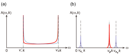
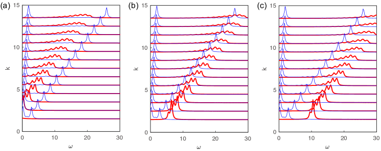
The two-point functions for fermions allow us to define the retarded Green’s function . From its Fourier transform, we can define the spectral weight , which vanishes when and . An example of spectral weights of and fermions (thin and thick lines, respectively) at fixed in this case is plotted in Fig. 1(a).
3.2 The case
At the special point , the model in the form of Eq. (LABEL:eq:LaF) becomes a free fermion model, with fermions and decoupled. The fermion has a linear dispersion . By changing the fermion to a momentum shifted basis , which eliminates the dependence of tunneling term , it splits into two chiral Bogoliubov fermionic modes and in the Nambu basis, where the fermion has a dispersion . The model in Eq. (LABEL:eq:LaF) in this case is thus integrable.
We derive below the two-point functions of different particles in this case for momentum difference . The generic case is discussed in Appendix C. 1. With , the two Bogoliubov modes can be recombined into two Majorana modes and with linear dispersions , where velocities . The two-point functions of the and fermions are simply free propagators:
| (6) | ||||
Their spectral weights are and , respectively, as shown in Fig. 1(b).
In the bosonic representation, with , the boson is free and thus has a correlation . The boson is not free, although splits into free Majorana fermions. It is thus easy to calculate the two-point function of the charge anyon operator , which reads . However, the calculation of two-point functions of the charge anyon operator and the electron operator are more complicated, due to the non-free nature of boson field . We now show that they can be calculated by doubling the model.
We define a double-copy of our model Lagrangian as , where is the Lagrangian defined in Eqs. (1) and (2) with boson fields and (). Accordingly, we perform a basis transformation for each copy, similar to Eq. (3). Next, we transform to a boson basis () defined by and , and define four complex fermion fields . This is known as the SO(8) triality transformation [43, 44, 45, 46, 47, 48, 28]. By further transforming into a new fermion basis , , and then do a bosonization to four boson fields (, ), one arrives at a free boson model (see App. C 2. b). The eigen-boson fields of this free boson model are where , under which the double-copy Lagrangian takes a diagonal form
| (7) |
The velocities are defined by , and , with and in Eq. (6).
We can now calculate the two-point functions of the charge anyon and the electron . Since the two copies we introduced are identical and decoupled, the two-point function of anyon can be rewritten as , where is the anyon operator in copy . Next, we note that the product operator , and are free bosons and decoupled with . Therefore, we only need to know the two-point function of operator , which can be derived from the two-point function of fermion . This enables us to express the anyon two-point function as , with given by Eq. (6). A similar transformation holds for the two-point function of electron . The two-point function of fermion can be calculated by transforming into the fermion basis , which yields in terms of the free bosons in Eq. (7). We therefore find the two-point function of anyon and electron given by (App. C. 2. b)
| (8) |
where , and the exponents , , .
4 The generic case
For generic parameters and , the model in Eq. (LABEL:eq:LaF) is difficult to solve, so we turn to study the model numerically with ED. To simplify the problem, we first eliminate factor of the tunneling term by a unitary transformation, at the price of adding a chemical potential. This is done by shifting the boson fields and in Eq. (3) into a new basis and , and define their corresponding fermion fields and . The Lagrangian in Eq. (LABEL:eq:LaF) then becomes (App. D. 1)
| (9) |
where the chemical potential . Since the fermion is neutral and the fermion carry charge , the term is equivalent to a physical chemical potential on the edge of the FQH state.
The model in the form of Eq. (9) has three apparent conserved global charges: (i) the total many-body momentum , (ii) the total charge of the fermion , and (iii) the parity of the fermion , which are explicitly given by
| (10) |
To perform ED calculations, we assume the 1D space is closed and has length , and we take an anti-periodic boundary condition for both the and fermions (which is the boundary condition for zero bulk flux). Since the chirality allows only positive momentum excitations, the Hilbert space dimension of each total momentum is finite, making our ED numerical calculation possible (see App. D. 2). For convenience, we set the unit of length such that . This constraints the single-particle momentum of the fermions to half-odd integers, i.e., . As a result, the many-body momentum is an integer (half-odd integer) if the total number of fermions is even (odd). Therefore, the three conserved charges , and are not independent, and we have
| (11) |
The charge sector has an additional special symmetry. To see this, we define a particle-hole transformation obeying
| (12) | ||||
When , becomes a symmetry of the Hamiltonian, which can have eigenvalues .
Therefore, the eigenstates of our model can be classified into global charge sectors labeled by when , and when .
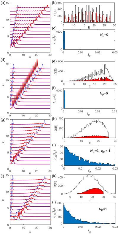
Noting that the term only shifts the energy spectrum of a global charge sector by a constant , thus we will not discuss much on the effect of . But does affect the spectral weights, which can be seen from Fig. 2 and App. D. 2. Fig. 2 shows a comparison among the numerical results of the case ((a)-(c)), the case ((d)-(f)), and the generic case with both and nonzero ((g)-(i) for , and (j)-(l) for ), with the total momentum up to , and the parameters are given in the Fig. 2 caption. In particular, we compute the many-body level spacing statistics (LSS) in each global charge sector, which is known to obey a Poisson distribution if the model is integrable [49], and obey a Wigner-Dyson distribution ( for Gaussian orthogonal, unitary and symplectic ensembles, respectively) if the model is fully chaotic in the charge sector [50, 51, 52].
In the case, Fig. 2(a) shows the spectral weights of fermion (red thick lines) and of fermion (blue thin lines) from ED, which matches well with the theoretical curves in Fig. 1(a) derived from the free boson picture. With a finite system size, the numerical spectral weights are a set of discrete delta functions, which we have broadened into Lorentzian functions (App. D. 2). In Fig. 2(b), we plot the density of states (DOS) at total momentum of all the sectors (black unfilled line) and of only the sector (red filled line). Fig. 2(c) shows the LSS in the sector, which is approximately a delta function (or Poisson distribution with an infinite decay exponent) because of the extensive level degeneracy of free bosons.
In the case, and are free fermions, and their ED spectral weights are delta functions as shown in Fig. 2(d), agreeing with the theoretical plot in Fig. 1(d). Similar to the case, the existence of enormous degenerate levels (Fig. 2(e)) leads to an approximate delta function LSS in each conserved () sector, as shown in Fig. 2(f).
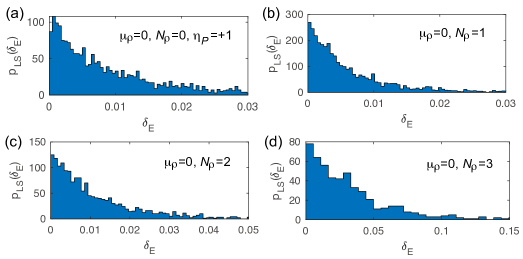
In the generic , case, the spectral weights of fermions , show behaviors in between the free boson and free fermion pictures, as shown in Fig. 2(g) and (j) (see more examples in App. D. 2). Accordingly, the DOS (Fig. 2(h),(k)) is smoother than that in the free boson and free fermion cases (Fig. 2(b),(e)). Most intriguingly, the LSS of each conserved global charge sector shows a Poisson statistics. Fig. 2(i) shows the LSS in the sector, and Fig. 2(l) shows the LSS of the () sector. More examples are given in App. D. 2 Fig. (4). Note that a nonzero in Eq. (9) will not change the LSS, which only globally shifts the energy of each sector. This suggests that there are more hidden local conserved quantities (local symmetries), or the generic model in Eq. (9) may in fact be quantum integrable if there are sufficient number of hidden local conserved quantities, which is an intriguing future problem. We note that the Poisson LSS in the generic case is still drastically different from the delta-function like LSS in the free boson and free fermion cases. This indicates that randomness exists in the energy spectrum of the generic case, unlike the free cases which yield extensively degenerate many-body energy levels.
5 The effect of irrelevant terms
Our model has been ignoring the irrelevant terms so far. Generically, if a model is integrable at low energies, irrelevant terms may lead to breaking of integrability at high energies. Examining such integrability breaking by irrelevant terms would also support that the Poisson LSS shown in our edge model is not an artefact of numerical calculation.
In this section, we introduce an irrelevant nonlinear term to the Lagrangian density of our edge model, which preserves all the global symmetries we have identified:
| (13) |
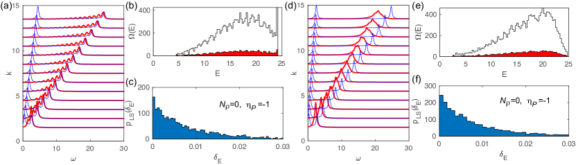
where is the coupling strength. This term gives an additional nonlinear dispersion relation for the free part of both the charged and neutral fermions. A simple dimension counting reveals that this nonlinear term is irrelevant and thus has vanishing effects on the low energy physics. To examine the effect of this term in Eq. (13) at high energies, one can either go to larger momentum or larger coupling strength , which are equivalent up to a scaling transformation. Numerically, it is easier to enlarge the coupling than the momentum .
It has been shown that by adding such nonlinear terms to the free chiral boson Luttinger liquid theory, the integrability will be broken at high energies as revealed by the LSS [53, 29]. Therefore, we expect a similar breaking of the potential integrability of our model by such irrelevant nonlinear terms here.
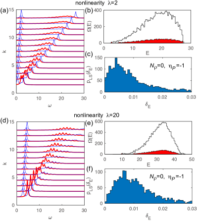
As shown in Fig. 3 (as compared with Fig. 2(i)), which are calculated from ED (see details in App. D. 2), when the coupling strength increases, the LSS in a global charge sector clearly shows a crossover from Poisson distribution to a Gaussian orthogonal ensemble (GOE) Wigner-Dyson distribution. The GOE type Wigner-Dyson LSS is due to the combined anti-unitary symmetry of our model, where is the spatial inversion and is the spinless time-reversal symmetry. This indicates that the irrelevant nonlinear term in Eq. 13 makes our model quantum chaotic at high energies, in contrast to the potentially integrable behavior at low energies. This also indicates that any hidden local conserved charges in each global charge sector will be broken by the irrelevant terms.
6 Discussion
We have shown that the generic FQH edge model is equivalent to an interacting fermion model with a -wave pairing in the neutral channel (Eq. (9)). It has two solvable points as free chiral bosons and free chiral (Majorana) fermions, respectively. It would be interesting to tune the system towards and momentum difference (by tuning the edge potentials and chemical potential), where three different velocities of free chiral fermions (one charge and two Majorana) emerge. For generic parameters, each conserved global charge and momentum sector shows a Poisson LSS in our ED calculation, suggesting the existence of more hidden local conserved quantities. This also suggests the possibility that the generic model is quantum integrable. On the other hand, adding irrelevant nonlinear kinetic terms shifts the LSS from Poisson to Wigner-Dyson at high energies, which also indicates that any hidden local conserved quantities we have not identified yet are only exact at low energies. Moreover, it will be interesting and important to understand if the hidden local conserved quantities could protect the quantum coherence and obstruct the thermalization of the FQH edge states, in contrast to quantum chaotic low-energy chiral edge theories [27, 28] where edge states are decoherent and fast scrambling. Further practical questions include if interference of different edges can be observed for the FQH chiral edge state, similar to that of the FQH state which was employed to measure the anyon braiding [13].
There are more FQH edge theories which exhibit a similar physics. For example, in the experimentally accessible regimes, the edge theory of the Halperin state [54, 55] at total filling also allows only one charge-conserving tunneling term with dimensionless coupling similar to Eq. (2), where , and no other tunneling term is more relevant. The other example is the Halperin state at total filling , which allows only one tunneling term of dimensionless coupling with . More series of such Abelian bilayer FQH states are identified in App. E. All of these models can be mapped into the fermion model in Eq. (LABEL:eq:LaF) and thus exhibit similar physics. An interesting future direction is to study chiral edge models allowing multiple tunneling terms with dimensionless couplings, which may not be mapped to a fermion model. One may ask if the competition between different tunneling terms (which are equally relevant) will bring testable robust quantum chaos at low energies.
Lastly, in our numerical ED calculations, we considered only pure FQH edges without any disorder. Disorder is certainly a significant aspect of FQH physics, however, it is difficult to be added to numerical calculations due to its momentum conservation breaking nature. Therefore, we leave it for future studies from more analytical perspectives. For a clean enough sample, our theoretical analysis with spatially uniform coupling and chemical potential can be regarded as a lowest order approximation keeping the mean values of the disordered potentials, which are more relevant than their fluctuations. Moreover, in FQH edge interference experiments [13], to maintain coherence, the length of edge is usually not too long. Disorder effects are thus expected to play less of a role in such conditions.
Acknowledgments. We thank for the helpful discussions with Duncan Haldane, Shivaji Sondhi and Bertrand Halperin. This work is supported by the Alfred P. Sloan Foundation, and NSF through the Princeton University’s Materials Research Science and Engineering Center DMR-2011750. Additional support was provided by the Gordon and Betty Moore Foundation through Grant GBMF8685 towards the Princeton theory program.
References
- DzyaloshinskiĬ and Larkin [1996] I. E. DzyaloshinskiĬ and A. I. Larkin, in 30 Years of the Landau Institute — Selected Papers (WORLD SCIENTIFIC, 1996) pp. 95–101.
- Haldane [1981a] F. D. M. Haldane, Journal of Physics C: Solid State Physics 14, 2585 (1981a).
- Haldane [1981b] F. D. M. Haldane, Phys. Rev. Lett. 47, 1840 (1981b).
- Tomonaga [1950] S. Tomonaga, Progress of Theoretical Physics 5, 544 (1950).
- Luttinger [1963] J. M. Luttinger, Journal of Mathematical Physics 4, 1154 (1963).
- Wen [1990] X. G. Wen, Phys. Rev. B 41, 12838 (1990).
- Wen [1991] X. G. Wen, Phys. Rev. B 43, 11025 (1991).
- Willett et al. [2009] R. L. Willett, L. N. Pfeiffer, and K. W. West, Proceedings of the National Academy of Sciences 106, 8853 (2009).
- Zhao et al. [2020] L. Zhao, E. G. Arnault, A. Bondarev, A. Seredinski, T. F. Q. Larson, A. W. Draelos, H. Li, K. Watanabe, T. Taniguchi, F. Amet, H. U. Baranger, and G. Finkelstein, Nature Physics 16, 862 (2020).
- Lian et al. [2016] B. Lian, J. Wang, and S.-C. Zhang, Phys. Rev. B 93, 161401 (2016).
- Roulleau et al. [2008] P. Roulleau, F. Portier, P. Roche, A. Cavanna, G. Faini, U. Gennser, and D. Mailly, Phys. Rev. Lett. 100, 126802 (2008).
- Laughlin [1983] R. B. Laughlin, Phys. Rev. Lett. 50, 1395 (1983).
- Nakamura et al. [2020] J. Nakamura, S. Liang, G. C. Gardner, and M. J. Manfra, Nature Physics 16, 931 (2020).
- Carrega et al. [2021] M. Carrega, L. Chirolli, S. Heun, and L. Sorba, Nature Reviews Physics (2021).
- McClure et al. [2012] D. T. McClure, W. Chang, C. M. Marcus, L. N. Pfeiffer, and K. W. West, Phys. Rev. Lett. 108, 256804 (2012).
- Ofek et al. [2010] N. Ofek, A. Bid, M. Heiblum, A. Stern, V. Umansky, and D. Mahalu, Proceedings of the National Academy of Sciences 107, 5276 (2010).
- Halperin et al. [2011] B. I. Halperin, A. Stern, I. Neder, and B. Rosenow, Phys. Rev. B 83, 155440 (2011).
- Kane et al. [1994] C. L. Kane, M. P. A. Fisher, and J. Polchinski, Phys. Rev. Lett. 72, 4129 (1994).
- Levin et al. [2007] M. Levin, B. I. Halperin, and B. Rosenow, Phys. Rev. Lett. 99, 236806 (2007).
- Lee et al. [2007] S.-S. Lee, S. Ryu, C. Nayak, and M. P. A. Fisher, Phys. Rev. Lett. 99, 236807 (2007).
- Lian and Wang [2018] B. Lian and J. Wang, Phys. Rev. B 97, 165124 (2018).
- Chamon and Wen [1994] C. d. C. Chamon and X. G. Wen, Phys. Rev. B 49, 8227 (1994).
- Wan et al. [2002] X. Wan, K. Yang, and E. H. Rezayi, Phys. Rev. Lett. 88, 056802 (2002).
- Wan et al. [2003] X. Wan, E. H. Rezayi, and K. Yang, Phys. Rev. B 68, 125307 (2003).
- Sabo et al. [2017] R. Sabo, I. Gurman, A. Rosenblatt, F. Lafont, D. Banitt, J. Park, M. Heiblum, Y. Gefen, V. Umansky, and D. Mahalu, Nature Physics 13, 491 (2017).
- Cano et al. [2014] J. Cano, M. Cheng, M. Mulligan, C. Nayak, E. Plamadeala, and J. Yard, Phys. Rev. B 89, 115116 (2014).
- Lian et al. [2019] B. Lian, S. L. Sondhi, and Z. Yang, Journal of High Energy Physics 2019 (2019), 10.1007/jhep09(2019)067.
- Hu and Lian [2022] Y. Hu and B. Lian, Phys. Rev. B 105, 125109 (2022).
- Schindler et al. [2022] F. Schindler, N. Regnault, and B. A. Bernevig, Phys. Rev. B 105, 035146 (2022).
- Martin and Matveev [2022] I. Martin and K. A. Matveev, Phys. Rev. B 105, 045119 (2022).
- Banerjee et al. [2018] M. Banerjee, M. Heiblum, V. Umansky, D. E. Feldman, Y. Oreg, and A. Stern, Nature 559, 205 (2018).
- Feldman [2018] D. E. Feldman, Phys. Rev. B 98, 167401 (2018).
- Simon [2018] S. H. Simon, Phys. Rev. B 97, 121406 (2018).
- Ma and Feldman [2019] K. K. W. Ma and D. E. Feldman, Phys. Rev. B 99, 085309 (2019).
- Boebinger et al. [1985] G. S. Boebinger, A. M. Chang, H. L. Stormer, and D. C. Tsui, Phys. Rev. Lett. 55, 1606 (1985).
- Lai et al. [2004] K. Lai, W. Pan, D. C. Tsui, and Y.-H. Xie, Phys. Rev. B 69, 125337 (2004).
- Ismail et al. [1995] K. Ismail, M. Arafa, K. L. Saenger, J. O. Chu, and B. S. Meyerson, Applied Physics Letters 66, 1077 (1995).
- Maiti et al. [2021] T. Maiti, P. Agarwal, S. Purkait, G. J. Sreejith, S. Das, G. Biasiol, L. Sorba, and B. Karmakar, Phys. Rev. B 104, 085304 (2021).
- Pudalov and Semenchinsky [1984] V. Pudalov and S. Semenchinsky, Solid State Communications 52, 567 (1984).
- Dean et al. [2011] C. R. Dean, A. F. Young, P. Cadden-Zimansky, L. Wang, H. Ren, K. Watanabe, T. Taniguchi, P. Kim, J. Hone, and K. L. Shepard, Nature Physics 7, 693 (2011).
- Hu et al. [2009] Z.-X. Hu, E. H. Rezayi, X. Wan, and K. Yang, Phys. Rev. B 80, 235330 (2009).
- Rozhansky et al. [2016] I. V. Rozhansky, N. S. Averkiev, and E. Lähderanta, Phys. Rev. B 93, 195405 (2016).
- Shankar [1981] R. Shankar, Phys. Rev. Lett. 46, 379 (1981).
- Shankar [1983] R. Shankar, Phys. Rev. Lett. 50, 787 (1983).
- Kane et al. [2020] C. L. Kane, D. Giuliano, and I. Affleck, Phys. Rev. Research 2, 023243 (2020).
- Ryu and Zhang [2012] S. Ryu and S.-C. Zhang, Phys. Rev. B 85, 245132 (2012).
- Maldacena and Ludwig [1997] J. M. Maldacena and A. W. Ludwig, Nuclear Physics B 506, 565 (1997).
- Fidkowski and Kitaev [2010] L. Fidkowski and A. Kitaev, Phys. Rev. B 81, 134509 (2010).
- Berry and Tabor [1977] M. V. Berry and M. Tabor, Proceedings of the Royal Society of London. A. Mathematical and Physical Sciences 356, 375 (1977).
- Bohigas et al. [1984] O. Bohigas, M. J. Giannoni, and C. Schmit, Phys. Rev. Lett. 52, 1 (1984).
- Dyson [1970] F. J. Dyson, Communications in Mathematical Physics 19, 235 (1970).
- Wigner [1967] E. P. Wigner, SIAM Review 9, 1 (1967).
- Lian [2022] B. Lian, arXiv e-prints , arXiv:2202.06169 (2022), arXiv:2202.06169 [cond-mat.str-el] .
- Halperin [1983] B. Halperin, Helv. Phys. Acta 56(1-3), 75 (1983).
- Halperin [1984] B. I. Halperin, Phys. Rev. Lett. 52, 1583 (1984).
Appendix A Fermionization of edge theory for the Quantum Hall state
The Lagrangian density describing the edge theory of the Abelian quantum Hall state is
| (14) |
with K-matrix , charge vector and is the real symmetric velocity matrix. For spatially uniform tunneling between these two edge modes, the leading interaction term is
| (15) |
where a momentum difference exist between the two modes adding a -dependent phase factor in the coupling strength . The hopping operator has scaling dimension two which renders the coupling constant dimensionless and non-negligible at low energies.
Our Lagrangian now becomes
| (16) |
We can further separate the neutral degrees of freedom from the charge degrees of freedom by the following basis transformation
| (17) |
characterized by vectors (transformation coefficients) and . Fermionizing as and , we obtain an equivalent interacting fermion model:
| (18) |
where electric charges and according to . The velocities are given by , and . We have taken the following convention for bosonization mappings with a point-splitting procedure in the -direction, the details of which can be found in Appendices of Refs. [27, 28]:
| (19) |
Appendix B Solvable point at
When , Eq. (16) becomes a free boson model
| (20) |
Let , we perform the following basis transformation for boson fields
| (21) |
This diagonalizes the above Lagrangian density and gives us
| (22) |
with and up to constant shifts of boson fields . Following from this, we have
| (23) | ||||
and thus (noting that and )
| (24) | ||||
From Eq. (17), we also have
| (25) | ||||
and thus the charge anyon and the charge electron have two-point functions
| (26) | ||||
For charge and neutral fermons and , and the original electron operator , we can work out their retarded Green’s functions and spectral weight functions. To this end, we work in Euclidean spacetime with imaginary time for calculation conveniences. Their Green’s function in momentum space is
| (27) | ||||
where . This integration can be further simplified to
| (28) |
by changing the variables of integration and . We have and assume . Analytically continuing , we find the retarded Green’s function:
| (29) |
The spectral weight is then
| (30) |
such that
| (31) |
For our cases, , , and .
Appendix C Solvable point at
C.1 Two-point functions for fermions with generic momentum difference
When , the neutral and charge fermions in Eq. (18) are completely decoupled. Let us define a new fermion operator , such that our Hamiltonian density becomes position independent:
| (32) |
Fourier transforming to momentum space, we have
| (33) |
We see that is with linear dispersion relation . For the neutral fermion , we can perform a Bogoliubov transformation
| (34) |
with
| (35) |
which gives us the spectrum of the Bogoliubov fermion :
| (36) |
For two-point function calculation conveniences, let us work in Euclidean spacetime with imaginary time . Since
| (37) |
the imaginary time ordered two-point function is defined as
| (38) |
where stands for time ordering. Fourier transforming the time direction gives us
| (39) |
where we have used
| (40) |
The real space Green’s function is thus
| (41) |
We can get the real-time Green’s function by analytically continuing and . The Green’s function of in the original basis is given by
| (42) |
C.2 Two-point correlation functions for fermions and anyons at
In this subsection, we calculate explicitly the correlation functions of fermions and anyons when .
C.2.1 For fermions
At , the calculation of two-point functions for fermions are straightforward. Let us again start with Euclidean spacetime for calculation conveniences. For fermions in charge sector, in momentum space, their two-point function is given as
| (43) |
Analytically continuing , we get the retarded Green’s function
| (44) |
which gives us the spectral weight function
| (45) |
Similarly, for fermions in neutral sector, we have the retarded Green function
| (46) |
where the velocities are given by . Then
| (47) |
signaling the appearance of two free Majorana fermions at . Fourier transforming back to real time domain, we have
| (48) |
C.2.2 For anyons
At , two-point correlation functions for the charge anyon can be readily calculated
| (49) |
For calculations of two-point correlation functions involving the charge anyon and the charge electron , we adapt a similar strategy implemented in [28]. We first enlarge our Hilbert space by making a duplicated copy of our Lagrangian density, after which the total Lagrangian reads
| (50) | ||||
where for each copy , we are in the neutral-charge basis defined as
| (51) |
Next, let us define new fermion variables such that
| (52) |
In literature [43, 44, 45, 46, 47, 48, 28], this is known as the triality transformation. Under this transformation, our Lagrangian density becomes
| (53) |
with velocity matrix
| (54) |
, and . In the fermion basis, the Lagrangian density is
| (55) |
This interacting fermion model can be further bosonized in a rotated fermion basis: , , such that all terms in the Lagrangian are bilinear in boson fields .
| (56) | ||||
with
| (57) |
and . Finally, we can diagonalize our Lagrangian density by changing to a new basis for boson fields: ,
| (58) |
with velocities
| (59) |
With the above exact mappings established, we have
| (60) | ||||
Since the charge degrees of freedom is always a free theory, we have
| (61) |
From the fact that , we have , which leads to
| (62) |
Since and , this gives us
| (63) | ||||
Appendix D Generic cases
In this section, we consider generic cases of edge theory (Eq. (16)) for the quantum Hall state with and .
D.1 The extra phase from momentum difference
The extra phase factor in Eq. (16) can be eliminated by performing an unitary transformation on boson fields such that we redefine them as
| (64) |
The price we pay is an additional chemical potential term with coefficient for the charge fermion generated from the above transformation. Putting these together, our Lagrangian density becomes
| (65) |
Green’s functions of both the neutral and charged fermions acquire pure phase factors in the new basis as a consequence:
| (66) |
This change does not alter results regarding level spacing statistics (LSS), and only shift the spectral weight functions of and fermions by a constant momentum.
D.2 Discretization and exact diagonlization
In this subsection, we discuss discretization procedures and other technical details for our exact diagonlization (ED) calculations for generic cases of our FQH chiral edge theory.
We model our edge theory as a closed one dimensional chiral system with total length and anti-periodic boundary condition for fermion operators and . Imposing anti-periodic boundary condition is natural when there is no flux inside the bulk. Under this set-up, we can Fourier transform the fermion operators to momentum space:
| (67) |
Our Hamiltonian in the real space is
| (68) |
Without loss of generality, we set , such that the fermion momentum . The Hamiltonian of our edge theory in real space can be transformed to momentum space as
| (69) | ||||
Because of the following relations between an electron operator and a hole operator:
| (70) |
by rewriting fermion operators with negative momentum as their hole operators, we can convert all the momentum of fermion operators in the summand of Eq. (69) as positive. Thus, for a given total many-body momentum , the Hilbert space dimension is finite, allowing us to employ the ED method to obtain the eigenstates and spectrum. To this end, the ground state of our Hamiltonian is the state with zero electrons and holes for both neutral () and charge () sectors. To further reduce redundant calculations, we need to identify symmetries of our Hamiltonian. We see three different conserved quantities: the total momentum , the total charge of charge fermion and the fermion parity of neutral fermions . Since , only two independent conserved quantities left and we can label states in our Hilbert space by which sector they belong. In the sectors, our model has an additional particle-hole symmetry as defined in Eq. (12), yielding another conserved charge (eigenvalues of ). Our ED calculations for the sector can thus be done for a global charge sector .
After we obtain the full spectrum, we can calculate the zero-temperature spectral weight function at a given momentum . It is defined as
| (71) |
where is the -th many-body eigenstate (sorted in the order of increasing energy) of total momentum sector of Eq. (69), which has energy , and is the Hilbert space dimension of the total momentum sector. It satisfies
| (72) |
To plot the spectral weight, we used a Lorentizan function in places for a Dirac delta function as
| (73) |
where we take for all our plots.
We also plot the level spacing statistics (LSS) of conserved charge sectors in Fig. (4) here and in Fig. (2) of the main text. For each conserved charge sector (or sector when ), assume the energy levels are with sorted in the energy increasing order. The LSS is then defined as the distribution of energy differences between consecutive energy levels
| (74) |
within sector .
In addition to Fig. (2) of our main text, we plotted spectral weight functions, density of states and level spacing statistics for more exmaples in Fig. (5) and Fig. (6) with various parameter settings. In Fig. (5), we added nonzero chemical potentials. We notice that the effect of chemical potential term is dominantly shifting the energy of the spectral weight of the fermion. In Fig. (6), the results display behaviours between that of a free boson theory and a free fermion theory.
The Hamiltonian for added nonlinear terms in momentum space is
| (75) |
Together with Eq. 69, our fermions have dispersion relations and .
Appendix E Other Abelian bilayer fermionic FQH systems
Although we have focused on the state for detailed analysis of its edge theory, there are many other Abelian bilayer FQH states with two-by-two K-matrix that can be solved in a similar fashion using the method presented in this paper. In this section, we present mathematical patterns of K-matrices of these states. We leave the generalization to larger matrices to the future studies.
We restrict ourselves in bilayer electronic systems, thus the K-matrix must have odd integers as diagonal entries. The other condition we impose is that the system has one (and only one) leading interaction term which describes electron hopping processes between the two chiral edges. Similar to Eq. (2) in main text, it assumes a form
| (76) |
where again originates from the momentum differences between the two edge modes, and we require the scaling dimension of to be two, so that the coupling constant is again dimensionless and non-negligible at low energies. Besides, this electron hopping process has to be electrically neutral, namely, charge conserving.
To be more explicit, for a generic two-by-two matrix with boson fields basis , we must have , and (as ground state degeneracy must be positive). The above conditions for the interaction term can be summarized as two equations for the two-component integer vector :
| (77) |
where the first equation fixes its scaling dimension to be two and the second equation ensures the interaction term is electrically neutral.
Putting on all these constraints, by an extensive search of solutions of Eq. (77), we find two classes of K-matrices, one for filling balanced bilayer systems, and the other for the filling imbalanced case.
For the balanced case, for each , at filling factor , we have a series of K-matrix
| (78) |
that satisfies the above characterizations with integer vector describing the marginal interaction term. We see that the -state [54, 55] is the first member of this series.
The imbalanced case is more complicated, we find three different series of K-matrices. The first series occur at filling factor for . There are two varieties,
| (79) |
with integer vector and
| (80) |
with integer vector and respectively. The -state is the second member () of the series.
The second series occurs at filling factor for .
| (81) |
with integer vector .
The third series occurs at filling factor for .
| (82) |
with integer vector .
We note here that the patterns found in this section are not meant to be complete. Besides, many examples followed from this pattern, taken as bilayer FQH systems, are not observed experimentally. This is partial due to the fact that their filling factors for each layer is smaller than . In these cases, physically, an energetically more dominant Wigner crystal phase or other competing phases may emerge.
