Constraints on star formation in NGC 2264

Abstract

We quantify the spatial distribution of stars for two subclusters centred around the massive/intermediate mass stars S Mon and IRS 1/2 in the NGC 2264 star-forming region. We find that both subclusters are have neither a substructured, nor a centrally concentrated distribution according to the $\mathcal{Q}$-parameter. Neither subcluster displays mass segregation according to the $\Lambda_{\rm MSR}$ ratio, but the most massive stars in IRS 1/2 have higher relative surface densities according to the $\Sigma_{\rm LDR}$ ratio. We then compare these quantities to the results of $N$-body simulations to constrain the initial conditions of NGC 2264, which are consistent with having been dense ($\tilde{\rho}\sim 10^{4}$ M_⊙ pc^-3), highly substructured and subvirial. These initial conditions were also derived from a separate analysis of the runaway and walkaway stars in the region, and indicate that star-forming regions within 1 kpc of the Sun likely have a broad range of initial stellar densities. In the case of NGC 2264, its initial stellar density could have been high enough to cause the destruction or truncation of protoplanetary discs and fledgling planetary systems due to dynamical encounters between stars in the early stages of its evolution.

1 Introduction

Stars form from the collapse and fragmentation of Giant Molecular Clouds, which usually results in groups or clusters of stars of a similar age and chemical composition (Lada & Lada, 2003). These groups tend to exhibit spatial and kinematic substructure at young ages (e.g. Gomez et al., 1993; Gouliermis et al., 2014; Foster et al., 2015; Buckner et al., 2019) as well as stellar densities that are between $10-10^{5}$ times as dense as the Sun’s current location in the Galaxy (Korchagin et al., 2003).

Because of their high densities, these star-forming regions tend to evolve on very short timescales ($\sim$1 Myr) and so establishing the initial conditions (e.g.  birth density, velocity distribution) can be problematic (Parker, 2014). The most effective way of establishing the initial conditions of a star-forming region is to “reverse engineer" the present-day observed spatial and kinematic distributions, i.e.  compare the current distributions to numerical simulations of the formation and evolution of star-forming regions.

In order to do this, an assumption has to be made about the universality of star-formation, i.e. a property must be fixed that is thought to be the general outcome of all star formation (such as the Initial Mass Function (IMF), Bastian et al., 2010). Some authors have assumed the primordial binary star population – like the IMF – is invariant, and therefore the amount of binary destruction places limits on the amount of dynamical evolution (Kroupa, 1995; Marks et al., 2011).

However, the observed binary populations suffer from high levels of incompleteness (Duchêne & Kraus, 2013), and furthermore, the narrow range of observed binaries in star-forming regions straddle the ‘Hard-Soft’ boundary (Heggie, 1975; Hills, 1975a, b), making it difficult to ascertain whether an observed binary population will have undergone dynamical processing, even if situated in a dense star-forming region (Parker & Goodwin, 2012).

As an alternative to binary stars, in previous work (Parker et al., 2014; Wright et al., 2014; Parker & Alves de Oliveira, 2017) we have attempted to constrain the initial conditions of star formation by assuming that each star-forming event results in a spatially and kinematically substructured distribution (where the level of substructure is allowed to vary), and use this substructure as a dynamical clock to compare to observations.

This earlier work focused exclusively on the spatial information, such as the overall structure (Cartwright & Whitworth, 2004; Cartwright, 2009) and the amount of mass segregation (Allison et al., 2009) or relative surface densities (Maschberger & Clarke, 2011; Parker et al., 2014). The Gaia satellite has facilitated a vast improvement in these comparisons by enabling the proper motions of runaway stars to be used as dynamical tracers of the regions’ past evolution (Schoettler et al., 2019; Farias et al., 2020; Schoettler et al., 2020).

Recently, Schoettler et al. (2020) used runaway ($>30$ km s^-1 and walkaway ($\gtrsim 10$ km s^-1) stars to confirm earlier structural analyses (Allison et al., 2009, 2010; Allison & Goodwin, 2011; Parker et al., 2014) that constrained the initial conditions of the Orion Nebula Cluster as being dense, substructured and subvirial. Using information from the proper motions of runaways and walkaways has the advantage over studies that quantify the radial velocity dispersion in that no correction for binary stars need be applied (Gieles et al., 2010; Cottaar et al., 2012).

In Schoettler et al. (2021) we applied this analysis to NGC 2264, which unlike the ONC is not a smooth centrally concentrated cluster. Indeed, NGC 2264 is referred to as the ‘Christmas Tree cluster’, due to its unusual spatial distribution. NGC 2264 has had at least two temporally distinct episodes of star formation, but Schoettler et al. (2021) was able to pinpoint the initial conditions of these two episodes and – like the ONC – found them to be consistent with dense ($10^{4}$ M_⊙ pc^-3), substructured and subvirial star-formation.

In this paper, we follow-up the analysis of NGC 2264 in Schoettler et al. (2021) to determine whether the spatial distribution of the stars in this region is also consistent with the analysis of the runaway and walkaway stars. This paper is organised as follows. In Section 2 we provide a description of the dataset, in Section 3 we describe the methods used to quantify the spatial distributions of stars, as well as describing the set-up of the $N$-body simulations we compare the data to. In Section 4 we present the results, we provide a discussion in Section 5 and we conclude in Section 6.

2 Observational data

We construct a mass census of stars that belong to NGC 2264 based on identified members from different surveys. The member surveys we use contain a larger number of stars than those we include into our mass census as some of these stars lack information on their stellar mass.

For the mass census, we identify members from the work of Venuti et al. (2017, 2018, 2019), who mainly focused on the low- to intermediate mass members of the cluster. Their work is mainly based on photometric observations from the “Coordinated Synoptic Investigation of NGC 2264” (CSI) 2264 project (Cody et al., 2014) in combination with data from other photometric and spectroscopic observational campaigns (e.g. SDSS, Gaia-ESO, IPHAS, Pan-STARRS1, Abazajian et al., 2009; Randich et al., 2013; Barentsen et al., 2014; Flewelling et al., 2020).

We find further members in Dahm et al. (2007) who used X-ray observations; Jackson et al. (2020) who used data from the Gaia-ESO campaign; Maíz Apellániz (2019) and Cantat-Gaudin & Anders (2020) who both used Gaia DR2 for their member identification. Where information about the membership probability was given, we use stars with a probability of 50 per cent or above as part of our census. As noted in Schoettler et al. (2021), while the members of NGC 2264 are fairly well constrained on-sky, they are far less constrained in their distance measurement. While the majority of the members are found around at a distance of around 700–800 pc, there are also identified members in several of the literature sources we use that show distances far above and below this value range. We do not exclude any of these members in our analysis, as a comparison of the Gaia DR2 and EDR3 parallaxes show that these measurements can change considerably between different observations (Gaia Collaboration et al., 2018; Gaia Collaboration et al., 2020).

Our final mass census contains 750 stars, either with a mass estimate or a spectral type, which we use to derive masses. NGC 2264 has an upper age estimate of around 5 Myr, which means that most of the stars in this cluster are still pre-main sequence stars. To convert pre-main sequence spectral types into mass estimates, we use the values in Table 2 from Kirk & Myers (2011) who follow the procedure introduced in Luhman et al. (2003) to estimate masses based on effective temperature.

However, the surveys we use to construct the mass census contain more stars identified as members but that do not have masses or spectral types and with membership probabilities below 50 per cent. The size of our mass census should therefore not be considered as equal to the current size of the cluster population. Depending on the level of interstellar extinction and how embedded the sources are, current observations are also unlikely to probe the full mass range down to 0.1 M_⊙, where a large number of possible member stars might still remain undetected. Venuti et al. (2019) identified a total of 1369 sources in the clustered population, of which only 54 stars had a clear identification as field stars. The others were either “very likely” or “possible” members of the cluster or had no membership flag at all. Teixeira et al. (2012) estimated the size of the stellar population in NGC 2264 within their search fields that contain all three of the regions of interest to contain 1436$\pm$242 members. This highlights that the current size of NGC 2264 is likely in the range of 1200 – 1450 members.

We show a map of the data in Fig. 1. The 750 stars in our sample are indicated by the grey points. We split the region into two sub-clusters, based on the observed age dichotomy in NGC 2264. In the upper, northern cluster surrounding the massive star S Mon, the stars have ages around 5 Myr, and in the lower, southern cluster surrounding the stars IRS 1 and IRS 2, the stars have ages around 2 Myr. Our assumption is that – whilst the stars may have formed from the same molecular cloud – there have been at least two epochs of star formation in NGC 2264 and we therefore split the region into two subclusters in order to perform our analysis.

In Fig. 1 we show the position of S Mon by the small blue circle, and the extent over which we perform our structural analyses by the larger blue circle, which has a radius of 0.168 degrees ($\sim$2 pc at the adopted distance to NGC 2264). Similarly, we show the positions of IRS 1 and IRS 2 in the southern subcluster by the small pink circles, and the extent over which we perform the structural analyses by the larger pink circle, which again has a radius of 0.158 degrees (we indicate the centre of this larger circle by the pink asterisk).

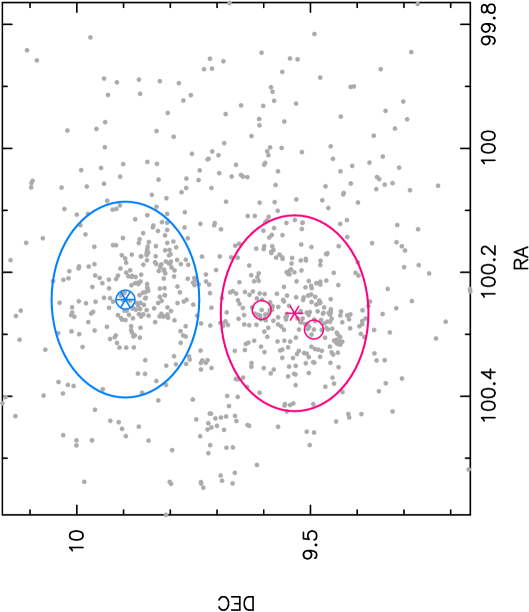
Figure 1: Map of NGC 2264 with the stars in our sample shown by the grey points. The most massive star in the upper subcluster (S Mon) is shown by the smaller blue circle, and the extent over which we perform the structural analysis for this subcluster is indicated by the larger blue circle (which has a radius of 0.158 degrees, or $\sim$2 pc). In the lower subcluster, the massive stars IRS 1 and IRS 2 are indicated by the small pink circles, and the region over which we perform the structural analysis is shown by the larger pink circle (which has a radius of 0.158 degrees, or $\sim$2 pc). The central position of this circle is indicated with an asterisk.

3 Method

In this section we describe the methods used to quantify the structure in NGC 2264 and in the $N$-body simulations, as well as the set-up of the $N$-body simulations.

3.1 Structural analyses

3.1.1 The $\mathcal{Q}$-parameter

We quantify the overall structure of each subcluster using the $\mathcal{Q}$-parameter (Cartwright & Whitworth, 2004; Cartwright, 2009; Lomax et al., 2011; Jaffa et al., 2017). The $\mathcal{Q}$-parameter is determined by constructing a minimum spanning tree (MST), which is a graph joining all of the points in a distribution via the shortest possible total path length and where there are no closed loops. We also construct the complete graph, in which every point is joined to every other point via a connecting line.

The $\mathcal{Q}$-parameter is the mean length of the MST, $\bar{m}$, divided by the mean edge length of the complete graph, $\bar{s}$:

$$\mathcal{Q}=\frac{\bar{m}}{\bar{s}}.$$ (1)

In two dimensions, $\mathcal{Q}<0.7$ indicates a clumpy, or substructured distribution, whereas $\mathcal{Q}>0.9$ indicates a smooth, centrally concentrated distribution. $\mathcal{Q}$ values in the range 0.7 – 0.9 indicate a distribution with neither a substructured nor a centrally concentrated distribution. Such a distribution may be uniform, but in reality an observed distribution (or from simulations) may be more complex.

The $\mathcal{Q}$-is formally scale-free, as $\bar{m}$ is normalised to

$$\frac{\sqrt{NA}}{N-1},$$ (2)

where $N$ is the number of points in the distribution and $A$ is the area of a circle with a radius $R$ equal to the magnitude of the furthest point from the origin. $\bar{s}$ is normalised to the radius $R$.

The normalisation to the radius generally means that the $\mathcal{Q}$-parameter is scale-free. There is a mild dependence of $\mathcal{Q}$ on the number of stars (Lomax et al., 2011; Parker & Dale, 2015; Parker, 2018), but the main degeneracy is when $\mathcal{Q}$ is calculated for a dataset with significant outliers, e.g.   stars that are tens of pc away from the main part of a star-forming region with a size scale of $\sim$1 pc. This is potentially an issue for our comparison with $N$-body simulations (Parker, 2014) and so we limit our analysis in our simulations to stars within two half-mass radii of the centre of the region.

3.1.2 The $\Lambda_{\rm MSR}$ mass segregation ratio

We quantify the degree of mass segregation using the Allison et al. (2009) $\Lambda_{\rm MSR}$ ratio. This constructs an MST between $N_{\rm MST}$ stars in a chosen subset to determine the length $l_{\rm subset}$ of this MST. We then compare this length with the average MST length of $N_{\rm MST}$ randomly chosen stars, $\langle l_{\rm average}\rangle$:

$$\Lambda_{\rm MSR}=\frac{\langle l_{\rm average}\rangle}{l_{\rm subset}}^{+\sigma_{5/6}/{l_{\rm subset}}}_{-\sigma_{1/6}/{l_{\rm subset}}},$$ (3)

where the lower (upper) uncertainty is the MST length which lies 1/6 (5/6) of the way through an ordered list of all the random lengths, which corresponds to a 66 per cent deviation from the median value, $\langle l_{\rm average}\rangle$ (Allison et al., 2009; Parker et al., 2011; Parker, 2018). This has the advantage that an outlying datapoint cannot strongly influence the uncertainty, although we in any case restrict our determination of $\Lambda_{\rm MSR}$ in the simulations to stars within two half-mass radii of the centre.

3.1.3 Local surface density

The local surface density, $\Sigma$, is determined for every star using the equation in Casertano & Hut (1985):

$$\Sigma=\frac{N-1}{\pi r_{N}^{2}},$$ (4)

where $N$ is the number of nearest neighbours and $r_{N}$ is the projected distance to the $N^{\rm th}$ nearest neighbour. The value of $\Sigma$ is fairly insensitive to the choice of $N$ (Bressert et al., 2010; Parker & Meyer, 2012), and we adopt $N=10$ here. The advantage of $\Sigma$ is that it can be used to directly compare the densities in simulated star-forming regions with observed regions.

Maschberger & Clarke (2011) introduced the $\Sigma-m$ plot to quantify differences between the surface density of the most massive stars and the surface density of all of the stars in a region. Küpper et al. (2011) and Parker et al. (2014) introduced the local density ratio, $\Sigma_{\rm LDR}$ as the ratio between the median surface density of the ten most massive stars, $\tilde{\Sigma}_{\rm 10}$, (or any other defined subset) and the median surface density of all of the stars in the region, $\tilde{\Sigma}_{\rm all}$:

$$\Sigma_{\rm LDR}=\frac{\tilde{\Sigma}_{\rm 10}}{\tilde{\Sigma}_{\rm all}},$$ (5)

the significance of which is quantified using a Kolmogorov-Smirnov test.

3.1.4 Binary stars

Few structural analyses using the $\mathcal{Q}$-parameter, $\Lambda_{\rm MSR}$ and $\Sigma_{\rm LDR}$ have been performed on distributions with a significant fraction of binary systems (although this is common in studies that use the 2-point correlation function, e.g. Larson, 1995; Simon, 1997; Kraus & Hillenbrand, 2008). Küpper et al. (2011) showed that a population of binary systems will slightly alter the $\mathcal{Q}$-parameter, by virtue of the extra (short) links present between stars. This is more complicated for observational data where information on the binary systems may be restricted to binaries with a certain range of separations (e.g. King et al., 2012a, b; Duchêne & Kraus, 2013). In Appendix A we show that the range of binary separations we are sensitive to has a negligible effect on the results.

3.2 $N$-body simulations

We set up and run $N$-body simulations of star-forming regions designed to mimic the subclusters in NGC 2264. In the observational sample, the two subclusters contain 212 and 258 objects within our chosen sub-cluster boundaries. However, our $N$-body simulations have a higher number of systems (725 systems for each of the two subclusters), for several reasons.

First, the observational sample we use for our analysis is limited to stars for which we have a mass estimate or could derive one from their spectral type. Literature estimates considering all possible members for NGC 2264 give suggest considerably higher numbers, which are within the numbers chosen for the $N$-body simulations (Teixeira et al., 2012; Venuti et al., 2019). Second, the observational samples are likely missing a proportion of stars with very low masses (0.1–0.3  M_⊙) due to extinction or the sources being embedded. Third, we only use observations from the mass census that are within a 2 pc radius around the centre of each subcluster, and so there will be stars that originated from these subclusters that have travelled beyond this (arbitrary) boundary, but are still bound to the subclusters. Typically, our $N$-body simulation expand and there are around 200 - 300 stars within the 2 pc radius.

3.2.1 Stellar systems

Our simulations each have $N=725$ stellar systems, with masses drawn from the Maschberger (2013) Initial Mass Function (IMF) with a probability distribution function of the form

$$p(m)\propto\left(\frac{m}{\mu}\right)^{-\alpha}\left(1+\left(\frac{m}{\mu}\right)^{1-\alpha}\right)^{-\beta},$$ (6)

where $\mu=0.2$ M_⊙ is the average stellar mass, $\alpha=2.3$ and $\beta=1.4$. We sample this IMF between 0.1 and 50 M_⊙.

Table 1: Binary properties of systems in our simulations, which are set up to mimic the distributions observed in the Galactic field. We show the spectral type of the primary mass, the main sequence mass range this corresponds to, the binary fraction $f_{\rm bin}$, and for stars less massive than 3 M_⊙ we show the mean separation $\bar{a}$, and the mean (${\rm log}\,\bar{a}$) and variance ($\sigma_{{\rm log}\,\bar{a}}$) of the log-normal fits to these distributions. OB stars ($m_{p}>$3.0 M_⊙) are not drawn from a log-normal distribution but instead are drawn from a log-uniform Öpik (1924) distribution in the range 0 - 50 au.

Spectral Type	Primary mass	$f_{\rm bin}$	$\bar{a}$	${\rm log}\,\bar{a}$	$\sigma_{{\rm log}\,\bar{a}}$	Ref.
M-dwarf	$0.10<m_{p}/$M${}_{\odot}\leq 0.45$	0.34	16 au	1.20	0.80	Bergfors et al. (2010); Janson et al. (2012)
F, G, K	$0.45<m_{p}/$M${}_{\odot}\leq 1.20$	0.46	50 au	1.70	1.68	Raghavan et al. (2010)
A	$1.20<m_{p}/$M${}_{\odot}\leq 3.00$	0.48	389 au	2.59	0.79	De Rosa et al. (2014)
OB	$m_{p}>$ 3.00 M⊙	1.00	Öpik	0 – 50 au	log-uniform	Sana et al. (2013)

We then select a random number $\mathcal{R}_{n}$ between 0 and 1 to determine whether a system is a single or binary. The binary fraction, $f_{\rm bin}$ is defined as

$$f_{\rm bin}=\frac{B+\ldots}{S+B+\ldots},$$ (7)

where $S$ and $B$ are the numbers of single and binary systems, respectively (we do not include triple or quadruple systems in the simulations, although they are certainly an important outcome of the star formation process, Tokovinin, 2008, 2018; Reipurth et al., 2014; Pineda et al., 2015).

In accordance with observations in the Galactic field we assign a binary fraction as a function of the stellar mass. For stars $m>3.00$ M_⊙, $f_{\rm bin}=1.00$ (Mason et al., 1998; Kouwenhoven et al., 2007; Sana et al., 2013), for stars $1.20\leq m\leq 3.00$, $f_{\rm bin}=0.48$ (De Rosa et al., 2014), for stars $0.84\leq m<1.20$, $f_{\rm bin}=0.46$ (Raghavan et al., 2010), for stars $0.45\leq m<0.84$, $f_{\rm bin}=0.45$ (Mayor et al., 1992) and for stars $0.10\leq m<0.45$, $f_{\rm bin}=0.34$ (Janson et al., 2012). If $\mathcal{R}_{n}<f_{\rm bin}$ for the mass range the star falls within then the stellar system is set to be a binary.

The distribution of binary semimajor axes is also a function of primary mass. Binaries with $m>3.00$ M_⊙ have semimajor axes drawn from a log-uniform Öpik (1924) distribution between 0 and 50 au, whereas all other systems are drawn from a lognormal distribution where the mean and variance is also a function of the primary mass in the binary. These values are summarised in Table 1 but are characterised by higher mean semimajor axes for more massive primary stars, moving to progressively lower mean semimajor axes for low-mass stars (De Rosa et al., 2014; Raghavan et al., 2010; Ward-Duong et al., 2015; Janson et al., 2012).

We determine the mass of the companion star in the binary by assuming a flat mass ratio distribution as observed in the Galactic field (Reggiani & Meyer, 2011, 2013). Eccentricities are also drawn from a flat distribution (Raghavan et al., 2010; Duchêne & Kraus, 2013), apart from binaries with semimajor axes less than 1 au, which are placed on circular ($e=0$) orbits.

3.2.2 Star forming regions

We distribute our stellar systems randomly in a box fractal distribution according to the method in Goodwin & Whitworth (2004). This method is detailed in many other works (e.g. Allison et al., 2010; Parker et al., 2014; Schoettler et al., 2020) and we refer the interested reader to those papers for details. In short, the amount of spatial substructure in the region is set by the fractal dimension, $D$, with lower values (e.g. $D=1.6$) corresponding to more substructure, whereas $D=3.0$ is a uniform spherical distribution.

The fractals are constructed by determining how many parent particles mature and produce child particles, with the substructured regions producing fewer child particles. Stellar velocities for the parent particles are drawn from a Gaussian with mean zero, and the children inherit these velocities plus a small random noise component that decreases with each successive generation of children in the fractal. This way, the stars in regions with a high degree of substructure have very correlated velocities on local scales, but on large scales the velocities can vary significantly, similar to the observed Larson (1981) relations.

Table 2: Summary of the initial conditions adopted for our simulations. The total number of stellar systems (single and binary) is fixed at $N=750$ but we vary the initial radius $r_{F}$, fractal dimension $D$ and virial ratio $\alpha_{\rm vir}$. The different combinations of radii and fractal dimension give different initial median stellar densities $\tilde{\rho}$, which in turn result in different (observable) median stellar surface densities, $\tilde{\Sigma}$.

Sim. ID	$r_{F}$	$D$	$\alpha_{\rm vir}$	$\tilde{\rho}$ (0 Myr)	$\tilde{\Sigma}$ (0 Myr)
16-03-1	1 pc	$1.6$	0.3	10 000 M⊙ pc-3	3000 stars pc-2
16-05-1	1 pc	$1.6$	0.5	10 000 M⊙ pc-3	3000 stars pc-2
30-03-1	1 pc	$3.0$	0.3	150 M⊙ pc-3	400 stars pc-2
30-05-1	1 pc	$3.0$	0.5	150 M⊙ pc-3	400 stars pc-2
16-03-5	5 pc	$1.6$	0.3	70 M⊙ pc-3	100 stars pc-2
16-05-5	5 pc	$1.6$	0.5	70 M⊙ pc-3	100 stars pc-2
20-03-5	5 pc	$2.0$	0.3	10 M⊙ pc-3	40 stars pc-2
20-05-5	5 pc	$2.0$	0.5	10 M⊙ pc-3	40 stars pc-2

Finally, the velocities of individual stars are scaled to the overall ‘bulk motion’ of the star-forming regions, as set by the virial ratio $\alpha_{\rm vir}=|\Omega|/\mathcal{K}$, where $\Omega$ and $\mathcal{K}$ are the total potential and kinetic energies, respectively. In accordance with observations that suggest star-forming regions are initially subvirial (e.g. Peretto et al., 2006; Foster et al., 2015), we set some simulations with $\alpha_{\rm vir}=0.3$, whereas others are set to $\alpha_{\rm vir}=0.5$ (virial equilibrium). A summary of the initial conditions is given in Table 2.

We evolve the star-forming regions using the kira integrator in Starlab (Portegies Zwart et al., 1999, 2001), which is a 4^th-order Hermite $N$-body code with block time-stepping. We include stellar and binary evolution in the simulations by utilising SeBa look-up tables, also in Starlab (Portegies Zwart & Verbunt, 1996, 2012). The simulations are evolved for 10 Myr, i.e.  well beyond the upper age estimate for the S Mon subcluster (5 Myr).

4 Results

4.1 Observational data

4.1.1 S Mon

We first determine the $\mathcal{Q}$-parameter and its constituent $\bar{m}$ and $\bar{s}$ for the S Mon subcluster. $\mathcal{Q}=0.83$ and $\bar{m}=0.51$ and $\bar{s}=0.61$, which is at the boundary between a substructured and a smooth distribution, although the plot of $\bar{m}-\bar{s}$ (Cartwright, 2009; Parker, 2018) tentatively indicates a fractal distribution with $D=2.6$.

In Fig. 2(a) we show the mass segregation ratio $\Lambda_{\rm MSR}$ as a function of the $N_{\rm MST}$ most massive stars. This plot clearly shows no significant deviation from unity, meaning that the most massive stars have the same spatial distribution as the average stars.

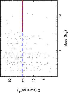
(a) S Mon

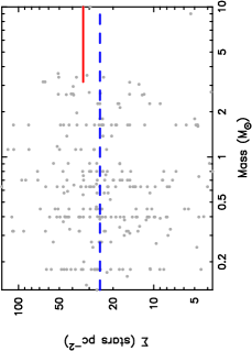
(b) IRS 1/2

Figure 3: The local surface density, $\Sigma$, as a function of stellar mass in each of the subclusters in NGC 2264. The blue dashed line is the median surface density for all of the stars in the subcluster, and the solid red line is the median surface density for the ten most massive stars. The ratio of these median densities is used to calculate the local surface density ratio, $\Sigma_{\rm LDR}$.

We show the local surface density as a function of mass for each star in Fig. 3(a). The median surface density for the region is 21 stars pc^-2 and the most massive stars have very similar values (compare the solid red line with the blue dashed line).

4.1.2 IRS 1/2

We now focus on the subcluster centred between the stars IRS 1 and IRS 2. The $\mathcal{Q}$-parameter and associated $\bar{m}$ and $\bar{s}$ values are 0.80, 0.61 and 0.76, respectively. Whilst this $\mathcal{Q}$-parameter is very much in the no-man’s land between being categorized as either substructured or smooth, the $\bar{m}$ and $\bar{s}$ values place it in the smooth, centrally concentred regime on the Cartwright (2009) plot.

In Fig. 2(b) we show the mass segregation ratio $\Lambda_{\rm MSR}$ as a function of the $N_{\rm MST}$ most massive stars. The 4 most massive stars do not deviate from a mass segregation ratio of unity, and although the 10 most massive stars have $\Lambda_{\rm MSR}=1.59^{+1.76}_{-1.24}$, we would caution against interpreting this as a significant signature of mass segregation (see Parker & Goodwin, 2015).

The median surface density for the IRS 1/2 subcluster is $\tilde{\Sigma}=24$ stars pc^-2, similar to the S Mon subcluster. However, the 10 most massive stars in IRS 1/2 do display a significant difference in their surface densities, as shown in Fig. 3(b) (compare the median surface density of the massive stars, shown by the red line, to the median surface density for all stars, shown by the blue dashed line). The KS test returns a $p$-value $p=3.6\times 10^{-2}$ that the two samples share the same underlying parent distribution.

Table 3: Summary of the results for the observed subclusters in NGC 2264. We show the number of stars in our dataset for each subcluster, $N$, the age, the mean length of the minimum spanning tree of each region, $\bar{m}$, the mean length of the complete graph for each region, $\bar{s}$, the $\mathcal{Q}$-parameter, the mass segregation ratio for the four most massive stars, $\Lambda_{\rm MSR,4}$, the mass segregation ratio for the ten most massive stars, $\Lambda_{\rm MSR,10}$, the median surface density for all stars in each subcluster, $\tilde{\Sigma}$, the local surface density ratio for the ten most massive stars, $\Sigma_{\rm LDR,10}$, and the KS test results between the surface densities of the ten most massive stars and the rest.

Subcluster	$N$	Age	$\bar{m}$	$\bar{s}$	$\mathcal{Q}$	$\Lambda_{\rm MSR,4}$	$\Lambda_{\rm MSR,10}$	$\tilde{\Sigma}$	$\Sigma_{\rm LDR,10}$	KS test
S Mon	212	5 Myr	0.51	0.61	0.83	0.71${}^{+0.80}_{-0.50}$	0.83${}^{+0.98}_{-0.83}$	21 stars pc-2	0.97	$D=0.24$, $p=0.56$
IRS 1/2	258	2 Myr	0.61	0.76	0.80	0.92${}^{+1.45}_{-0.73}$	1.59${}^{+1.76}_{-1.24}$	24 stars pc-2	1.33	$D=0.44$, $p=3.6\times 10^{-2}$

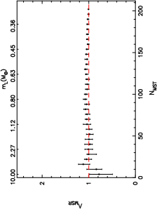
(a) S Mon

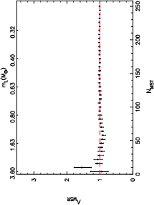
(b) IRS 1/2

Figure 2: The mass segregation ratio, $\Lambda_{\rm MSR}$, as a function of the $N_{\rm MST}$ most massive stars in each of the subclusters in NGC 2264. The lowest mass star in the $N_{\rm MST}$ subset is indicated on the top axis. The horizontal red dashed line indicates $\Lambda_{\rm MSR}=1$, i.e.  no mass segregation.

4.2 $N$-body simulations

We first provide an example of a simulation whose structural parameters ($\mathcal{Q}$-parameter, surface density $\Sigma$, mass segregation ratio $\Lambda_{\rm MSR}$ and local surface density ratio $\Sigma_{\rm LDR}$) provide a good fit to the observational data for the S Mon and IRS 1/2 subclusters in NGC2264. These properties are shown in Fig. 4 for a simulation (‘16-03-1’ in Table 2) with an initial radius of 1 pc, a high degree of substructure ($D=1.6$) and subvirial bulk motion ($\alpha_{\rm vir}=0.3$).

This simulation has a high initial surface density ($\Sigma=3000$ stars pc^-2), and undergoes subvirial collapse. As it collapses, the initial substructure is erased and the net effect is for the surface density to decrease (Fig 4(a)) and the $\mathcal{Q}$-parameter to increase (Fig. 4(b)). These simulations attain a small degree of mass segregation quantified as $\Lambda_{\rm MSR}>1$, shown in Fig. 4(c) and the massive stars attain moderately high local surface densities ($\Sigma_{\rm LDR}>1$, see Fig. 4(d)).

In this figure, we show the observed values for S Mon via the blue triangles, and for IRS 1/2 via the pink heptagons. In general, the simulation data are shown by grey lines/points, save for when the individual simulations also produce the same numbers of runaway and walkaway stars to the observed subclusters (Schoettler et al., 2021). In that case, the simulations are shown by blue lines/points (S Mon) or pink lines/points (IRS 1/2).

In Fig. 5 we show an example of a simulation in which the numbers of runaway and walkaway stars produced were categorically inconsistent with the numbers of observed RW/WW stars from both S Mon and IRS 1/2. These simulations (labelled ‘20-03-5’ in Table 2) have an initial radius of 5 pc, a moderate amount of spatial and kinematic substructure ($D=2.0$) and subvirial bulk motion ($\alpha_{\rm vir}=0.3$).

The combination of large radius and moderate substructure means that these simulations take much longer to dynamically evolve, such that the substructure is still present after 10 Myr of the simulation (note the low $\mathcal{Q}$-parameters in Fig. 5(b), which are inconsistent with the observed values). Whilst the median surface densities in these simulations are likely consistent with the observed value of S Mon (the blue triangle in Fig. 5(a)), the observed $\mathcal{Q}$-parameters in the simulations strongly suggest that the two subclusters are more dynamically evolved. This also means that the simulations do not fall within the area occupied by the observations in the $\mathcal{Q}-\Lambda_{\rm MSR}$ (Fig. 5(c)) and $\mathcal{Q}-\Sigma_{\rm LDR}$ (Fig. 5(d)) plots.

The two sets of simulations presented in Figs. 4 and 5 are very much extrema within the full set of simulations. In Table 4 we provide an overview of whether other simulations are also consistent with both the numbers of runaways and walkaways (RW/WW), and the various structural diagnostics. For a parameter where the simulations are consistent with the observations, we place a ‘Y’ in the table. For a parameter that is inconsistent with the observations, we place an ‘N’, and where it is ambiguous we place an ‘?’. We then sum the number of positives (‘Y’s) to determine how consistent each simulation is with the observations and we deem the simulations with the maximum number of positives to be the best fit to the data.

When we do this simplistic tallying, we find that the simulations most consistent with the observations are those that start with compact ($r_{F}=1$ pc) and substructured ($D=1.6$) initial conditions, which are very dense ($10^{4}$ M_⊙ pc^-3). The initial bulk motion can either be subvirial ($\alpha_{\rm vir}=0.3$) or in virial equilibrium ($\alpha_{\rm vir}=0.5$); in fact, this is a weak constraint because the local velocity dispersions in the substructure are usually highly subvirial (Parker & Wright, 2016, 2018). These compact, highly substructured initial conditions are also the optimal initial conditions identified from the RW/WW analysis in Schoettler et al. (2021).

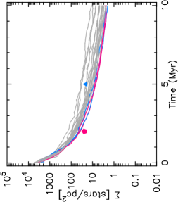
(a) $\Sigma$

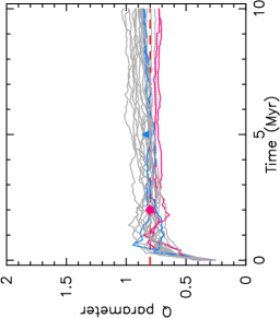
(b) $\mathcal{Q}$-parameter

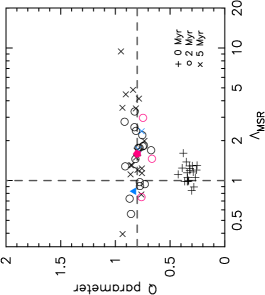
(c) $\mathcal{Q}-\Lambda_{\rm MSR}$

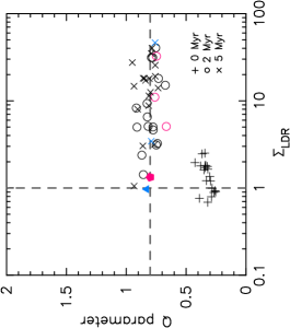
(d) $\mathcal{Q}-\Sigma_{\rm LDR}$

Figure 4: Results from $N$-body simulations with highly substructured ($D=1.6$), subvirial ($\alpha_{\rm vir}=0.3$) initial conditions where the star-forming regions have initial radii of 1 pc (labelled 16-03-1 in Table 2). In all panels the pink pentagon corresponds to the observed values for the IRS 1/2 subcluster and the blue triangle corresponds to the observed values for the S Mon subcluster. The pink lines and symbols are simulations where the numbers of runaways and walkaways are consistent with the observed values for IRS 1/2 at the upper age limit for this subcluster and the blue lines and symbols are simulations where the numbers of runaways and walkaways are consistent with the observed values for S Mon at the upper age limit for this subcluster. Panel (a) shows the evolution of the median local surface density, $\tilde{\Sigma}$ and panel (b) shows the evolution of the $\mathcal{Q}$-parameter [the horizontal red dashed line indicates the boundary between substructured ($\mathcal{Q}<0.8$) and smooth ($\mathcal{Q}>0.8$) morphologies]. In panel (c) we show the $\mathcal{Q}$-parameter and $\Lambda_{\rm MSR}$ values at 0, 2 and 5 Myr and in panel (d) we show the $\mathcal{Q}$-parameter and $\Sigma_{\rm LDR}$ values at 0, 2 and 5 Myr. The horizontal lines in panels (c) and (d) show the boundary between substructured and smooth morphologies according to the $\mathcal{Q}$-parameter, and the vertical lines indicate $\Lambda_{\rm MSR}=1$ (panel c) and $\Sigma_{\rm LDR}=1$ (panel d).

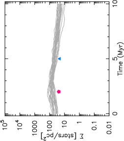
(a) $\Sigma$

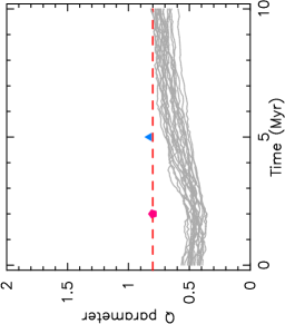
(b) $\mathcal{Q}$-parameter

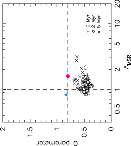
(c) $\mathcal{Q}-\Lambda_{\rm MSR}$

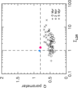
(d) $\mathcal{Q}-\Sigma_{\rm LDR}$

Figure 5: Results from $N$-body simulations with moderately substructured ($D=2.0$), subvirial ($\alpha_{\rm vir}=0.3$) initial conditions where the star-forming regions have initial radii of 5 pc (labelled 20-03-5 in Table 2). In all panels the pink pentagon corresponds to the observed values for the IRS 1/2 subcluster and the blue triangle corresponds to the observed values for the S Mon subcluster. None of these simulations produce the observed numbers of runaways and walkways from these subclusters. Panel (a) shows the evolution of the median local surface density, $\tilde{\Sigma}$ and panel (b) shows the evolution of the $\mathcal{Q}$-parameter [the horizontal red dashed line indicates the boundary between substructured ($\mathcal{Q}<0.8$) and smooth ($\mathcal{Q}>0.8$) morphologies]. In panel (c) we show the $\mathcal{Q}$-parameter and $\Lambda_{\rm MSR}$ values at 0, 2 and 5 Myr and in panel (d) we show the $\mathcal{Q}$-parameter and $\Sigma_{\rm LDR}$ values at 0, 2 and 5 Myr. The horizontal lines in panels (c) and (d) show the boundary between substructured and smooth morphologies according to the $\mathcal{Q}$-parameter, and the vertical lines indicate $\Lambda_{\rm MSR}=1$ (panel c) and $\Sigma_{\rm LDR}=1$ (panel d).

Table 4: Summary of the results from the $N$-body simulations. The columns show the simulation ID, the subcluster, and then whether each quantity from the simulations is consistent with the observed values. The first of these columns is whether the numbers of runaway/walkaway stars (RW/WW) in Schoettler et al. (2021) match the observed values, then the subsequent columns are the various structural parameters we calculate in this paper. Good fits to the observations are indicated by a ‘Y’, whereas marginal fits are indicated by an ‘?’ and bad fits are indicated by an ‘N’. The final columns are the total number of good fits, (a) just considering structure $n_{\rm fit}$ (structure only), and (b) with the runaway/walkaway constraints from Schoettler et al. (2021, $n_{\rm fit}$ with RW/WW).

Sim. ID	Subcluster	RW/WW	$\tilde{\Sigma}$	$\mathcal{Q}$	$\mathcal{Q}-\Lambda_{\rm MSR}$	$\mathcal{Q}-\Sigma_{\rm LDR}$	$n_{\rm fit}$ (structure only)	$n_{\rm fit}$ with RW/WW
16-03-1	S Mon	Y	Y	Y	Y	?	3+?	4+?
16-03-1	IRS 1/2	Y	Y	Y	Y	?	3+?	4+?
16-05-1	S Mon	Y	Y	Y	Y	?	3+?	4+?
16-05-1	IRS 1/2	Y	Y	Y	Y	N	3	4
30-03-1	S Mon	N	N	Y	N	Y	2	2
30-03-1	IRS 1/2	N	N	Y	Y	Y	3	3
30-05-1	S Mon	N	?	Y	N	Y	2+?	2+?
30-05-1	IRS 1/2	?	N	Y	Y	Y	3	3+?
16-03-5	S Mon	N	Y	Y	Y	N	3	3
16-03-5	IRS 1/2	?	N	N	N	N	0	0+?
16-05-5	S Mon	N	Y	Y	N	N	2	2
16-05-5	IRS 1/2	N	N	N	N	N	0	0
20-03-5	S Mon	N	Y	N	N	N	1	1
20-03-5	IRS 1/2	N	N	N	N	N	0	0
20-05-5	S Mon	N	Y	N	N	N	1	1
20-05-5	IRS 1/2	N	N	N	N	N	0	0

5 Discussion

5.1 Caveats and assumptions

The main assumption behind our simulations is the idea that star-forming regions always form with substructure. Dynamical interactions almost always erase substructure, and so the amount of substructure in a star-forming region can be used as a dynamical clock (e.g. Scally & Clarke, 2002; Goodwin & Whitworth, 2004; Parker & Meyer, 2012; Parker et al., 2014; Daffern-Powell & Parker, 2020), which is the underlying principle in the structural analysis presented here.

Both observations (André et al., 2010) and simulations (Bate, 2009) indicate that star-forming regions are clumpy and filamentary in their early stages, and this appears to translate into a substructured distribution for the pre-main sequence stars (Gomez et al., 1993; Larson, 1995; Cartwright & Whitworth, 2004; Cartwright, 2009). However, it is not clear how appropriate the box-fractal method is for mimicking this substructure (e.g. Lomax et al., 2018).

Our simulations are also devoid of any remaining gas from the star formation process, which could change the dynamical evolution of the subclusters if rapidly expelled by feedback from the massive stars (e.g. Tutukov, 1978; Goodwin, 1997; Baumgardt & Kroupa, 2007; Shukirgaliyev et al., 2018; Dinnbier & Walch, 2020).

In NGC 2264 there appear to have been multiple episodes of star formation, with the S Mon subcluster appearing to be older than IRS 1/2. We have analysed the same $N$-body simulations and applied the results to both subclusters (albeit at their respective ages). A more realistic approach would be to model the entire NGC 2264 region self-consistently, although such a simulation would need to be fine-tuned to account for the different bursts of star formation.

We emphasise again that we have elected to split NGC 2264 into two separate subclusters, based on the different ages of the subclusters in question. Hetem & Gregorio-Hetem (2019) analysed the overall structure of the entire NGC 2264 region and determined the $\mathcal{Q}$-pararameter, $\Lambda_{\rm MSR}$ and $\Sigma_{\rm LDR}$ ratios for all of the stars. This means that we cannot directly compare our results to theirs. However, our values are broadly consistent with those derived by Hetem & Gregorio-Hetem (2019) for the entire NGC 2264 region, with minimal evidence for a different spatial distribution for the most massive stars.

5.2 The initial conditions of star formation in NGC 2264

Based on the numbers of runaways and walkways stars in Gaia DR2 and Gaia EDR3, Schoettler et al. (2021) postulated that the initial density of both the S Mon and IRS 1/2 subclusters in NGC 2264 was likely to be of order $10^{4}$ M_⊙ pc^-3, and furthermore that this star-forming region was consistent with substructured and subvirial initial conditions.

Our structural analyses is also consistent with these initial conditions, with the possible exception of the $\mathcal{Q}-\Sigma_{\rm LDR}$ plots, which could indicate a marginally less dense set of initial conditions ($\geq 1000$ M_⊙ pc^-3). This is because in our simulations, stars that have spatially correlated velocities tend to group around the most massive stars, leading to elevated relative local surface densities for the most massive stars. However, if a dataset is incomplete, or affected by extinction, the $\Sigma_{\rm LDR}$ ratio could be reduced.

In terms of other nearby star-forming regions on which similar analyses have been performed, NGC 2264 appears to have had much more dense initial conditions than IC 348 (Parker & Alves de Oliveira, 2017), $\rho$ Oph (Parker et al., 2012; Parker et al., 2014) and Cyg OB2 (Wright et al., 2014), but comparable initial conditions to the ONC (Parker et al., 2014; Schoettler et al., 2020) and NGC 1333 (Parker & Alves de Oliveira, 2017).

Although just a handful of star-forming regions, these results indicate that nearby star-forming regions do not have a common initial stellar density, but rather a range of initial densities. At the high end, regions with densities $\sim 10^{4}$ M_⊙ pc^-3 could truncate protoplanetary discs via direct interactions (Scally & Clarke, 2002; Vincke et al., 2015; Vincke & Pfalzner, 2016; Portegies Zwart, 2016; Winter et al., 2018a), although significant destruction/alteration of the disc population via truncation only occurs if these densities are maintained for several Myr (Vincke & Pfalzner, 2018; Winter et al., 2018b).

In our simulations that reproduce the observed numbers of runaway and walkaway stars from NGC 2264, and match the observed surface density, structure and levels of mass segregation, the initial average volume densities are high ($\tilde{\rho}=10^{4}$ M_⊙ pc^-3), but rapidly decrease to $\tilde{\rho}=100$ M_⊙ pc^-3. In this scenario, some initial disc truncation could occur, but this is likely to be short-lived.

However, if planets have already been able to form at these young ages (which recent observations appear to confirm, e.g. Alves et al., 2020; Segura-Cox et al., 2020), they are likely to have their orbits affected at densities in the range $100-1000$ M_⊙ pc^-3 (Adams et al., 2006; Parker & Quanz, 2012). At the lower end of the scale, regions with densities $<100$ M_⊙ pc^-3 could still affect planet formation if massive stars are present due to Far Ultra Violet (FUV) radiation from stars more massive than 10 M_⊙, which can lead to photoevaporation of protoplanetary discs (Scally & Clarke, 2002; Adams et al., 2004; Concha-Ramírez et al., 2019; Nicholson et al., 2019; Parker et al., 2021). Given that S Mon and IRS 1 are both more massive than 10 M_⊙ (e.g. Peretto et al., 2006; Maíz Apellániz, 2019), photoevaporation has almost certainly altered protoplanetary discs in NGC 2264.

6 Conclusions

We have quantified the spatial structure of two subclusters within the NGC 2264 star-forming region, S Mon and IRS 1/2, as well as calculating the amount of mass segregation according to $\Lambda_{\rm MSR}$ and the relative local surface densities of the massive stars, $\Sigma_{\rm LDR}$. We then compared these quantities to the output of $N$-body simulations to constrain the initial conditions for star formation in NGC 2264. Our conclusions are the following:

(i) Both S Mon and IRS 1/2 have moderate $\mathcal{Q}$-parameters ($\mathcal{Q}\sim 0.8$), which indicates neither a substructured nor a very centrally concentrated distribution. Neither subcluster exhibits mass segregation according to $\Lambda_{\rm MSR}$, but the younger IRS 1/2 subcluster does exhibit a significantly high local surface density ratio for the most massive stars ($\Sigma_{\rm LDR}>1$).

(ii) When compared to $N$-body simulations, we find that both regions are consistent with high initial densities ($\tilde{\rho}\sim 10^{4}$ M_⊙ pc^-3), a high degree of initial substructure and (sub)virial initial velocities (under the assumption that star formation must always produce a filamentary/substructured distribution).

(iii) These initial conditions are also those that best match the numbers of runaway ($>30$ km s^-1) and walkaway ($>5$ km s^-1) stars observed with Gaia (Schoettler et al., 2021), suggesting that analysis of the spatial structure is consistent with analysis of the proper motion velocities of stars.

(iv) Our constraints suggest high initial densities for star formation in NGC 2264, commensurate with similar estimates for the ONC. At these densities, protoplanetary discs and fledgling planetary systems could be greatly affected by dynamical encounters and photoevaporation from the FUV radiation fields from massive stars.

In similar previous analyses we have found that such high initial densities are not observed/postulated for all star-forming regions, however, providing further evidence that ongoing star formation in the Milky Way results in a range of different densities (and by extension, different initial conditions for fledgling planetary systems).

Data Availability Statement

The data underlying this article were accessed from the Gaia archive, https://gea.esac.esa.int/archive/. The derived data generated in this research will be shared on reasonable request to the corresponding author.

Appendix A Binary systems

The structural diagnostics we apply to the observed and simulated data ($\mathcal{Q}$, $\Lambda_{\rm MSR}$ and $\Sigma_{\rm LDR}$) could in principle be biased by the binary star population. In the observational data, we have little or no information on whether each individual star is a binary, yet in order to make a meaningful assessment of the initial conditions, we require our simulations to include a population of primordial binary stars.

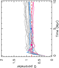
(a) 10 au cut, $\mathcal{Q}$-parameter

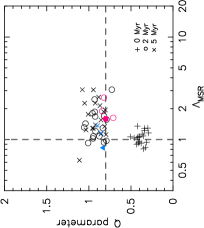
(b) 10 au cut, $\mathcal{Q}-\Lambda_{\rm MSR}$

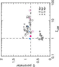
(c) 10 au cut, $\mathcal{Q}-\Sigma_{\rm LDR}$

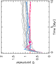
(d) 1000 au cut, $\mathcal{Q}$-parameter

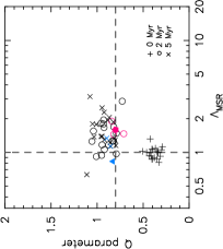
(e) 1000 au cut, $\mathcal{Q}-\Lambda_{\rm MSR}$

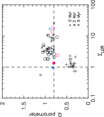
(f) 1000 au cut, $\mathcal{Q}-\Sigma_{\rm LDR}$

Figure 6: More results from $N$-body simulations with highly substructured ($D=1.6$), subvirial ($\alpha_{\rm vir}=0.3$) initial conditions where the star-forming regions have initial radii of 1 pc (labelled 16-03-1 in Table 2, and shown in Fig. 4). We have reanalysed these simulations by assuming binary systems with semimajor axes $a<10$ au would be observed as single stars (top row, panels (a)–(c)) and then again assuming binary systems with semimajor axes $a<1000$ au would be observed as single stars (bottom row, panels (d)–(f)). In all panels the pink pentagon corresponds to the observed values for the IRS 1/2 subcluster and the blue triangle corresponds to the observed values for the S Mon subcluster. The pink lines and symbols are simulations where the numbers of runaways and walkaways are consistent with the observed values for IRS 1/2 at the upper age limit for this subcluster and the blue lines and symbols are simulations where the numbers of runaways and walkaways are consistent with the observed values for S Mon at the upper age limit for this subcluster. Panels (a) and (d) show the evolution of the $\mathcal{Q}$-parameter [the horizontal red dashed line indicates the boundary between substructured ($\mathcal{Q}<0.8$) and smooth ($\mathcal{Q}>0.8$) morphologies]. Panels (b) and (e) show the $\mathcal{Q}$-parameter and $\Lambda_{\rm MSR}$ values at 0, 2 and 5 Myr and panels (c) and (f) show the $\mathcal{Q}$-parameter and $\Sigma_{\rm LDR}$ values at 0, 2 and 5 Myr. The horizontal lines in panels (b), (c), (e) and (f) show the boundary between substructured and smooth morphologies according to the $\mathcal{Q}$-parameter, and the vertical lines indicate $\Lambda_{\rm MSR}=1$ (panels (b) and (e)) and $\Sigma_{\rm LDR}=1$ (panels (c) and (f)).

Küpper et al. (2011) show that the $\mathcal{Q}$-parameter is slightly sensitive the the adopted binary population, but both $\Lambda_{\rm MSR}$ and $\Sigma_{\rm LDR}$ have not been tested in distributions that contain binaries. Moreover, because the binary population in NGC 2264 is largely unknown, we have reproduced the analysis of our best-fitting simulation ($r_{F}=1$ pc, $D=1.6$, $\alpha_{\rm vir}=0.3$, Fig. 4) under the assumption that we can resolve the individual components of binaries with separations greater than 10 au (panels (a)–(c) in Figs. 6) or 1000 au (panels (d)–(f) in Fig. 6). If a binary has a separation less than one of these thresholds, we count the system as a single star (in terms of its mass, and position), whereas if the binary separation exceeds these thresholds, we treat the components as two separate stars.

Fig. 6 clearly shows that selecting a separation threshold for binaries makes minimal differences to the outcome of the analysis and so we simply run our analysis on the population of stars within twice the half-mass radius from the subcluster centres, as described in Section 3.2.

References

- Abazajian et al. (2009) Abazajian K. N., et al., 2009, ApJS, 182, 543
- Adams et al. (2004) Adams F. C., Hollenbach D., Laughlin G., Gorti U., 2004, ApJ, 611, 360
- Adams et al. (2006) Adams F. C., Proszkow E. M., Fatuzzo M., Myers P. C., 2006, ApJ, 641, 504
- Allison & Goodwin (2011) Allison R. J., Goodwin S. P., 2011, MNRAS, 415, 1967
- Allison et al. (2009) Allison R. J., Goodwin S. P., Parker R. J., Portegies Zwart S. F., de Grijs R., Kouwenhoven M. B. N., 2009, MNRAS, 395, 1449
- Allison et al. (2010) Allison R. J., Goodwin S. P., Parker R. J., Portegies Zwart S. F., de Grijs R., 2010, MNRAS, 407, 1098
- Alves et al. (2020) Alves F. O., Cleeves L. I., Girart J. M., Zhu Z., Franco G. A. P., Zurlo A., Caselli P., 2020, ApJ, 904, L6
- André et al. (2010) André P., et al., 2010, A&A, 518, L102
- Barentsen et al. (2014) Barentsen G., et al., 2014, MNRAS, 444, 3230
- Bastian et al. (2010) Bastian N., Covey K. R., Meyer M. R., 2010, ARA&A, 48, 339
- Bate (2009) Bate M. R., 2009, MNRAS, 392, 590
- Baumgardt & Kroupa (2007) Baumgardt H., Kroupa P., 2007, MNRAS, 380, 1589
- Bergfors et al. (2010) Bergfors C., et al., 2010, A&A, 520, A54
- Bressert et al. (2010) Bressert E., et al., 2010, MNRAS, 409, L54
- Buckner et al. (2019) Buckner A. S. M., et al., 2019, A&A, 622, A184
- Cantat-Gaudin & Anders (2020) Cantat-Gaudin T., Anders F., 2020, A&A, 633, A99
- Cartwright (2009) Cartwright A., 2009, MNRAS, 400, 1427
- Cartwright & Whitworth (2004) Cartwright A., Whitworth A. P., 2004, MNRAS, 348, 589
- Casertano & Hut (1985) Casertano S., Hut P., 1985, ApJ, 298, 80
- Cody et al. (2014) Cody A. M., et al., 2014, AJ, 147, 82
- Concha-Ramírez et al. (2019) Concha-Ramírez F., Wilhelm M. J. C., Portegies Zwart S., Haworth T. J., 2019, MNRAS, p. arXiv:1907.03760
- Cottaar et al. (2012) Cottaar M., Meyer M. R., Parker R. J., 2012, A&A, 547, A35
- Daffern-Powell & Parker (2020) Daffern-Powell E. C., Parker R. J., 2020, MNRAS, 493, 4925
- Dahm et al. (2007) Dahm S. E., Simon T., Proszkow E. M., Patten B. M., 2007, AJ, 134, 999
- De Rosa et al. (2014) De Rosa R. J., et al., 2014, MNRAS, 437, 1216
- Dinnbier & Walch (2020) Dinnbier F., Walch S., 2020, MNRAS, 499, 748
- Duchêne & Kraus (2013) Duchêne G., Kraus A., 2013, ARA&A, 51, 269
- Farias et al. (2020) Farias J. P., Tan J. C., Eyer L., 2020, ApJ, 900, 14
- Flewelling et al. (2020) Flewelling H. A., et al., 2020, ApJS, 251, 7
- Foster et al. (2015) Foster J. B., et al., 2015, ApJ, 799, 136
- Gaia Collaboration et al. (2018) Gaia Collaboration et al., 2018, A&A, 616, A1
- Gaia Collaboration et al. (2020) Gaia Collaboration Brown A. G. A., Vallenari A., Prusti T., de Bruijne J. H. J., Babusiaux C., Biermann M., 2020, arXiv e-prints, p. arXiv:2012.01533
- Gieles et al. (2010) Gieles M., Sana H., Portegies Zwart S. F., 2010, MNRAS, 402, 1750
- Gomez et al. (1993) Gomez M., Hartmann L., Kenyon S. J., Hewitt R., 1993, AJ, 105, 1927
- Goodwin (1997) Goodwin S. P., 1997, MNRAS, 286, 669
- Goodwin & Whitworth (2004) Goodwin S. P., Whitworth A. P., 2004, A&A, 413, 929
- Gouliermis et al. (2014) Gouliermis D. A., Hony S., Klessen R. S., 2014, MNRAS, 439, 3775
- Heggie (1975) Heggie D. C., 1975, MNRAS, 173, 729
- Hetem & Gregorio-Hetem (2019) Hetem A., Gregorio-Hetem J., 2019, MNRAS, 490, 2521
- Hills (1975a) Hills J. G., 1975a, AJ, 80, 809
- Hills (1975b) Hills J. G., 1975b, AJ, 80, 1075
- Jackson et al. (2020) Jackson R. J., et al., 2020, MNRAS, 496, 4701
- Jaffa et al. (2017) Jaffa S. E., Whitworth A. P., Lomax O., 2017, MNRAS, 466, 1082
- Janson et al. (2012) Janson M., et al., 2012, ApJ, 754, 44
- King et al. (2012a) King R. R., Parker R. J., Patience J., Goodwin S. P., 2012a, MNRAS, 421, 2025
- King et al. (2012b) King R. R., Goodwin S. P., Parker R. J., Patience J., 2012b, MNRAS, 427, 2636
- Kirk & Myers (2011) Kirk H., Myers P. C., 2011, ApJ, 727, 64
- Korchagin et al. (2003) Korchagin V. I., Girard T. M., Borkova T. V., Dinescu D. I., van Altena W. F., 2003, AJ, 126, 2896
- Kouwenhoven et al. (2007) Kouwenhoven M. B. N., Brown A. G. A., Portegies Zwart S. F., Kaper L., 2007, A&A, 474, 77
- Kraus & Hillenbrand (2008) Kraus A. L., Hillenbrand L. A., 2008, ApJ, 686, L111
- Kroupa (1995) Kroupa P., 1995, MNRAS, 277, 1491
- Küpper et al. (2011) Küpper A. H. W., Maschberger T., Kroupa P., Baumgardt H., 2011, MNRAS, 417, 2300
- Lada & Lada (2003) Lada C. J., Lada E. A., 2003, ARA&A, 41, 57
- Larson (1981) Larson R. B., 1981, MNRAS, 194, 809
- Larson (1995) Larson R. B., 1995, MNRAS, 272, 213
- Lomax et al. (2011) Lomax O., Whitworth A. P., Cartwright A., 2011, MNRAS, 412, 627
- Lomax et al. (2018) Lomax O., Bates M. L., Whitworth A. P., 2018, MNRAS, 480, 371
- Luhman et al. (2003) Luhman K. L., Stauffer J. R., Muench A. A., Rieke G. H., Lada E. A., Bouvier J., Lada C. J., 2003, ApJ, 593, 1093
- Maíz Apellániz (2019) Maíz Apellániz J., 2019, A&A, 630, A119
- Marks et al. (2011) Marks M., Kroupa P., Oh S., 2011, MNRAS, 417, 1684
- Maschberger (2013) Maschberger T., 2013, MNRAS, 429, 1725