MonoScene: Monocular 3D Semantic Scene Completion

Abstract

MonoScene proposes a 3D Semantic Scene Completion (SSC) framework, where the dense geometry and semantics of a scene are inferred from a single monocular RGB image. Different from the SSC literature, relying on 2.5 or 3D input, we solve the complex problem of 2D to 3D scene reconstruction while jointly inferring its semantics. Our framework relies on successive 2D and 3D UNets, bridged by a novel 2D-3D features projection inspired by optics, and introduces a 3D context relation prior to enforce spatio-semantic consistency. Along with architectural contributions, we introduce novel global scene and local frustums losses. Experiments show we outperform the literature on all metrics and datasets while hallucinating plausible scenery even beyond the camera field of view. Our code and trained models are available at https://github.com/cv-rits/MonoScene.

1 Introduction

Estimating 3D from an image is a problem that goes back to the roots of computer vision [54]. While we, humans, naturally understand a scene from a single image, reasoning all at once about geometry and semantics, this was shown remarkably complex by decades of research [80, 57, 75]. Subsequently, many algorithms use dedicated depth sensors such as Lidar [36, 62, 50] or depth cameras [15, 2, 19], easing the 3D estimation problem. These sensors are often more expensive, less compact and more intrusive than cameras which are widely spread and shipped in smartphones, drones, cars, etc. Thus, being able to estimate a 3D scene from an image would pave the way for new applications.

3D Semantic Scene Completion (SSC) addresses scene understanding as it seeks to jointly infer its geometry and semantics. While the task gained popularity recently [56], the existing methods still rely on depth data (i.e. occupancy grids, point cloud, depth maps, etc.) and are custom designed for either indoor or outdoor scenes.

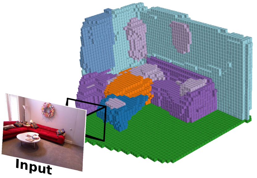
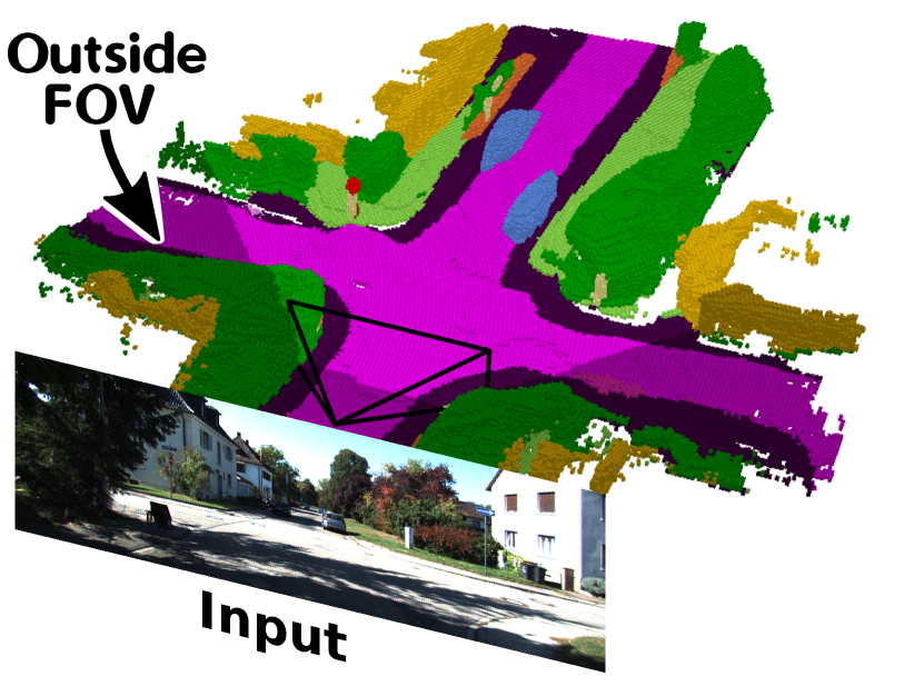
Indoor (NYUv2[58])	Outdoor (SemanticKITTI [3])

Figure 1: RGB Semantic Scene Completion with MonoScene. Our framework infers dense semantic scenes, hallucinating scenery outside the field of view of the image (dark voxels, right).

Here, we present MonoScene which – unlike the literature – relies on a single RGB image to infer the dense 3D voxelized semantic scene working indifferently for indoor and outdoor scenes. To solve this challenging problem, we project 2D features along their line of sight, inspired by optics, bridging 2D and 3D networks while letting the 3D network self-discover relevant 2D features. The SSC literature mainly relies on cross-entropy loss which considers each voxel independently, lacking context awareness. We instead propose novel SSC losses that optimize the semantic distribution of group of voxels, both globally and in local frustums. Finally, to further boost context understanding, we design a 3D context layer to provide the network with a global receptive field and insights about the voxels semantic relations. We extensively tested MonoScene on indoor and outdoor, see Fig. 1, where it outperformed all comparable baselines and even some 3D input baselines. Our main contributions are summarized as follows.

• MonoScene: the first SSC method tackling both outdoor and indoor scenes from a single RGB image.

• A mechanism for 2D Features Line of Sight Projection bridging 2D and 3D networks (FLoSP, Sec. 3.1).

• A 3D Context Relation Prior (3D CRP, Sec. 3.2) layer that boosts context awareness in the network.

• New SSC losses to optimize scene-class affinity (Sec. 3.3.1) and local frustum proportions (Sec. 3.3.2).

2 Related works

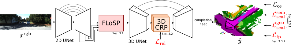
Figure 2: MonoScene framework. We infer 3D SSC from a single RGB image, leveraging 2D and 3D UNets, bridged by our Features Line of Sight Projection (FLoSP Sec. 3.1), and a 3D Context Relation Prior (3D CRP, Sec. 3.2) to enhance spatio-semantic awareness. On top of standard cross-entropy ($\mathcal{L}_{\text{ce}}$), our Scene-Class Affinity loss ($\mathcal{L}_{\text{scal}}$, Sec. 3.3.1) improves the global semantics ($\mathcal{L}^{\text{sem}}_{\text{scal}}$) and geometry ($\mathcal{L}^{\text{geo}}_{\text{scal}}$), and our Frustums Proportion loss ($\mathcal{L}_{\text{fp}}$, Sec. 3.3.2) enforces class distribution in local frustums, providing supervision beyond occlusions.

3D from a single image. Despite early researches [80, 31, 57], in the deep learning era the first works focused on single 3D object reconstruction with explicit [66, 67, 16, 65, 26, 1, 23, 70, 63, 11, 43] or implicit representations [49, 47, 51, 68, 52]. A comprehensive survey on the matter is [30]. For multiple objects, a common practice is to couple reconstruction with object detection [34, 35, 27, 78, 28]. Closer to our work, holistic 3D understanding seeks to predict the scene and objects layout [48, 32, 75, 37, 60, 83], reaching a sparse scene representation. Only [18] recently addressed indoor dense visible panoptic reconstruction by backprojecting individual 2D task features to 3D. We instead densely estimate semantics and geometry for both indoor and outdoor scenarios.

3D semantic scene completion (SSC). SSCNet [59] first defined the ‘SSC’ task where geometry and semantics are jointly inferred. The task gained attention lately, and is thoroughly reviewed in a survey [56]. Existing works all use geometrical inputs like depth [45, 40, 25, 42, 41, 39, 12], occupancy grids [25, 55, 13, 69] or point cloud [81, 53]. Truncated Signed Distance Function (TSDF) were also proved informative [59, 77, 20, 21, 10, 64, 79, 41, 9, 12, 6]. Among others originalities, some SSC works use adversarial training to guide realism [64, 10], exploit multi-task [38, 6], or use lightweight networks [40, 55]. Of interest for us, while others have used RGB as input [29, 14, 45, 40, 25, 20, 8, 20, 42, 9, 39, 81, 6] it is always along other geometrical input (e.g. depth, TSDF, etc.). A remarkable point in [56] is that existing methods are designed for either indoor or outdoor, performing suboptimally in the other setting. The same survey highlights the poor diversity of losses for SSC. Instead, we address SSC only using a single RGB image, with novel SSC losses, and are robust to various types of scenes.

Contextual awareness. Contextual features are crucial for semantics [71] and SSC [56] tasks. A simple strategy is to concatenate multiscale features with skip connections [59, 77, 19, 9, 45] or use dilated convolutions for large receptive fields [73], for example with the popular Atrous Spatial Pyramid Pooling (ASPP) [7] also used in SSC [45, 55, 40, 39]. Long-range information is gathered by self-attention in [33, 24] and global pooling in [72, 76]. Explicit contextual learning is shown to be beneficial in [71]. We propose a 3D contextual component that leverages multiple relation priors and provides a global receptive field.

3 Method

3D Semantic Scene Completion (SSC) aims to jointly infer geometry and semantics of a 3D scene $\hat{y}$ by predicting labels $C=\{c_{0},c_{1},\dots,c_{M}\}$, being free class $c_{0}$ and $M$ semantic classes. This has been almost exclusively addressed with 2.5D or 3D inputs [56], such as point cloud, depth or else, which act as strong geometrical cues.

Instead, MonoScene solves voxel-wise SSC from a single RGB image $x^{\text{rgb}}$, learning $\hat{y}=f(x^{\text{rgb}})$. This is significantly harder due to the complexity of recovering 3D from 2D. Our pipeline in Fig. 2 uses 2D and 3D UNets bridged by our Features Line of Sight Projection module (FLoSP, Sec. 3.1), lifting 2D features to plausible 3D locations, that boosts information flow and enables 2D-3D disentanglement. Inspired by [71], we capture long-range semantic context with our 3D Context Relation Prior component (3D CRP, Sec. 3.2) inserted between the 3D encoder and decoder. To guide the SSC training, we introduce new complementary losses. First, a Scene-Class Affinity Loss (Sec. 3.3.1) optimizes the intra-class and inter-class scene-wise metrics. Second, a Frustum Proportion Loss (Sec. 3.3.2) aligns the classes distribution in local frustums, which provides supervision beyond scene occlusions.

2D-3D backbones. We rely on consecutive 2D and 3D UNets with standard skip connections. The 2D UNet bases on a pre-trained EfficientNetB7 [61] taking as input the image $x^{\text{rgb}}$. The 3D UNet is a custom shallow encoder-decoder with 2 layers. The SSC output $\hat{y}$ is obtained by processing the 3D UNet output features with our completion head holding a 3D ASPP [7] block and a softmax layer.

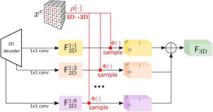
Figure 3: Features Line of Sight Projection (FLoSP). We project multi-scale 2D features $\mathsf{F}^{\text{1:s}}_{\text{2D}}$ (here, $s\in\{1,2,4,8\}$) along their line of sight by sampling ($\Phi(\cdot)$) them where the 3D voxels centroids ($x^{c}$) project ($\rho(\cdot)$). This boosts the 2D-3D information flow, and lets the 3D network discover which 2D features are relevant.

3.1 Features Line of Sight Projection (FLoSP)

Lifting 2D to 3D is notoriously ill-posed due to the scale ambiguity of single view point [22]. We rather reason from optics and backproject multiscale 2D features to all possible 3D correspondences, that is along their optical ray, aggregated in a unique 3D representation. Our intuition here is that processing the latter with a 3D network will provide guidance from the ensemble of 2D features. Our projection mechanism is akin to [52] but the latter projects each 2D map to a given 3D map – acting as 2D-3D skip connections. In contrast, our component bridges the 2D and 3D networks by lifting multiscale 2D features to a single 3D feature map. We argue this enables 2D-3D disentangled representations, providing the 3D network with the freedom to use high-level 2D features for fine-grained 3D disambiguation. Compared to [52], ablation in Sec. 4.3 shows our strategy is significantly better.

Our process is illustrated in Fig. 3. In practice, assuming known camera intrinsics, we project 3D voxels centroids ($x^{\text{c}}$) to 2D and sample corresponding features from the 2D decoder feature map $\mathsf{F}^{1:s}_{\text{2D}}$ of scale $1{:}s$. Repeating the process at all scales $S$, the final 3D feature map $\mathsf{F}_{\text{3D}}$ writes

$$\mathsf{F}_{\text{3D}}=\sum_{s\in S}\Phi_{\rho(x^{\text{c}})}(\mathsf{F}^{1\text{:}s}_{\text{2D}})\,,$$ (1)

where $\Phi_{a}(b)$ is the sampling of $b$ at coordinates $a$, and $\rho(\cdot)$ is the perspective projection. In practice, we backproject from scales $S{=}\{1,2,4,8\}$, and apply a 1x1 conv on 2D maps before sampling to allow summation. Voxels projected outside the image have their feature vector set to 0. The output map $\mathsf{F}_{\text{3D}}$ is used as 3D UNet input.

(a) Voxel$\leftrightarrow$Voxel relations

	free		occ
	f${}_{\textbf{s}}$	f${}_{\textbf{d}}$	o${}_{\textbf{s}}$	o${}_{\textbf{d}}$
$\leftrightarrow$	✓	✓	✗	✗
$\leftrightarrow$	✗	✓	✗	✗
$\leftrightarrow$	✗	✗	✓	✓

(a) Samples Supervoxel$\leftrightarrow$Voxel relations.

Figure 4: 2D illustration of 4-way relations. 4(a) We consider voxel$\leftrightarrow$voxel relations whether one is free or both are occupied, and if their semantics is similar or different. 1(a) For memory reason, we encode Supervoxel$\leftrightarrow$Voxel relations framed as multi-label classification. ( free, occupied - colors denote semantics)

3.2 3D Context Relation Prior (3D CRP)

Because SSC is highly dependent on the context [56], we inspire from CPNet [71] that demonstrates the benefit of binary context prior for 2D segmentation. Here, we propose a 3D Context Relation Prior (3D CRP) layer, inserted at the 3D UNet bottleneck, which learns n-way voxel$\leftrightarrow$voxel semantic scene-wise relation maps. This provides the network with a global receptive field, and increases spatio-semantic awareness due to the relations discovery mechanism.

Because SSC is a highly imbalanced task, learning binary (i.e. $n{=}2$) relations as in [71] is suboptimal. We instead consider $n{=}4$ bilateral voxel$\leftrightarrow$voxel relations, grouped into free and occupied corresponding to ‘at least one voxel is free’ and ‘both voxels are occupied’, respectively. For each group, we encode whether the voxels semantic classes are similar or different, leading to the 4 non-overlapping relations: $\mathcal{M}{=}\{\textbf{f}_{\textbf{s}},\textbf{f}_{\textbf{d}},\textbf{o}_{\textbf{s}},\textbf{o}_{\textbf{d}}\}$.  Fig. 4(a) illustrates the relations in 2D (see caption for colors meaning).

As voxels relations are greedy with $N^{2}$ relations for $N$ voxels, we present the lighter supervoxel$\leftrightarrow$voxel relations.

Supervoxel$\leftrightarrow$Voxel relation.  We define supervoxels as non-overlapping groups of $s^{3}$ neighboring voxels each, and learn the smaller supervoxel$\leftrightarrow$voxel relation matrices of size $\frac{N^{2}}{s^{3}}$. Considering a supervoxel $\mathcal{V}$ having voxels $\{\nu_{1},\dots,\nu_{s^{3}}\}$ and a voxel $\nu$, there are $s^{3}$ pairwise relations $\{\nu_{1}{\leftrightarrow}\nu,\dots,\nu_{s^{3}}{\leftrightarrow}\nu\}$. Instead of regressing the complex count of $\mathcal{M}$ relations in $\mathcal{V}{\leftrightarrow}\nu$, we predict which of the $\mathcal{M}$ relations exist, as depicted in Tab. 1(a). This writes,

$$\mathcal{V}{\leftrightarrow}\nu=\{\nu_{1}{\leftrightarrow}\nu,\dots,\nu_{s^{3}}{\leftrightarrow}\nu\}_{\neq},$$ (2)

where $\{\cdot\}_{\neq}$ returns distinct elements of a set.

3D Context Relation Prior Layer. Fig. 5 illustrates the architecture of our layer. It takes as input a 3D map of spatial dimension $H\mathsf{x}\mskip 1.0mu{}W\mathsf{x}\mskip 1.0mu{}D$, on which is applied a serie of ASPP convolutions [7] to gather a large receptive field, then split into $n{=}|\mathcal{M}|$ matrices of size $HWD{\times}\frac{HWD}{s^{3}}$.

Each matrix $\hat{A}^{m}$ encodes a relation $m{\in}{M}$, supervised by its ground truth $A^{m}$. We then optimize a weighted multi-label binary cross entropy loss:

$$\mathcal{L}_{rel}{=}{-}\sum_{m\in\mathcal{M},i}[(1\text{-}A^{m}_{i})\log(1\text{-}\hat{A}^{m}_{i})\text{+}w_{m}A^{m}_{i}\log\hat{A}^{m}_{i}],$$ (3)

where $i$ loops through all elements of the relation matrix and $w_{m}=\frac{\sum_{i}(1-A^{m}_{i})}{\sum_{i}A^{m}_{i}}$. The relation matrices are multiplied with reshaped supervoxels features to gather global context.

Alternatively, relations in $A^{m}$ can be self-discovered (w/o $\mathcal{M}$) by removing $\mathcal{L}_{\text{rel}}$, i.e. behaving as attention matrices.

Figure 5: 3D Context Relation Prior (3D CRP). We infer relation matrices $\hat{A}^{m}$ (here, 4), where each encodes a unique relation ${m\in\mathcal{M}}$ – optionally supervised with a relation loss ($\mathcal{L}_{\text{rel}}$). The matrices are multiplied with the supervoxels features to gather context, and later combined (concate, conv, DDR [40]) with input features. The feature dimension is omitted for clarity.

3.3 Losses

We now introduce new losses pursuing distinct global (Sec. 3.3.1) or local (Sec. 3.3.2) optimization objectives.

3.3.1 Scene-Class Affinity Loss

We seek to explicitly let the network be aware of the global SSC performance. To do so, we build upon the 2D binary affinity loss in [71] and introduce a multi-class version directly optimizing the scene- and class- wise metrics.

Specifically, we optimize the class-wise derivable (P)recision, (R)ecall and (S)pecificity where $P_{c}$ and $R_{c}$ measure the performance of similar class $c$ voxels, and $S_{c}$ measures the performance of dissimilar voxels (i.e. not of class $c$). Considering $p_{i}$ the ground truth class of voxel $i$, and $\hat{p}_{i,c}$ its predicted probability to be of class $c$, we define:

$$P_{c}(\hat{p},p) =\log\frac{\sum_{i}\hat{p}_{i,c}\llbracket p_{i}=c\rrbracket}{\sum_{i}\hat{p}_{i,c}},$$ (4)

$$R_{c}(\hat{p},p) =\log\frac{\sum_{i}\hat{p}_{i,c}\llbracket p_{i}=c\rrbracket}{\sum_{i}\llbracket p_{i}=c\rrbracket},$$ (5)

$$S_{c}(\hat{p},p) =\log\frac{\sum_{i}({1-\hat{p}_{i,c}})(1-\llbracket p_{i}=c\rrbracket)}{\sum_{i}(1-\llbracket p_{i}=c\rrbracket)},$$ (6)

with $\llbracket.\rrbracket$ the Iverson brackets. For more generality, our loss $\mathcal{L}_{\text{scal}}$ maximizes the above class-wise metrics with:

$$\mathcal{L}_{\text{scal}}(\hat{p},p)=-\frac{1}{C}\sum_{c=1}^{C}({P_{c}(\hat{p},p)}+{R_{c}(\hat{p},p)}+{S_{c}(\hat{p},p)}).$$ (7)

In practice, we optimize semantics $\mathcal{L}^{\text{sem}}_{\text{scal}}{=}\mathcal{L}_{\text{scal}}(\hat{y},y)$ and geometry $\mathcal{L}^{\text{geo}}_{\text{scal}}{=}\mathcal{L}_{\text{scal}}(\hat{y}^{\text{geo}},y^{\text{geo}})$, where $\{y,y^{\text{geo}}\}$ are semantic and geometric labels with respective predictions $\{\hat{y},\hat{y}^{\text{geo}}\}$.

3.3.2 Frustum Proportion Loss

Figure 6: Frustum Proportion Loss. Considering an image divided into same-size 2D patches (here, $2{\times}2$), each corresponds to a 3D frustum in the scene, we align the predicted frustum class probabilities (e.g. $\hat{P}^{k}$) with the corresponding ground truth ($P^{k}$). This provides cues to the network for occlusions disambiguation.

Disambiguation of occlusions is impossible from a single viewpoint and we observe that occluded voxels tend to be predicted as part of the object that shadows them. To mitigate this effect, we propose a Frustum Proportion Loss that explicitly optimizes the class distribution in a frustum.

As illustrated in Fig. 6, rather than optimizing the camera frustum distribution, we divide the input image into $\ell{\times}\ell$ local patches of equal size and apply our loss on each local frustum (defined as the union of the individual pixels frustum in the patch). Intuitively, aligning the frustums distributions provide additional cues to the network on the scene visible and occluded structure, giving a sense of what is likely to be occluded (eg. cars are likely to occlude road).

Given a frustum $k$, we compute $P_{k}$ the ground truth class distribution of voxels in $k$, and $P_{k,c}$ the proportion of class $c$ in $k$. Let $\hat{P}_{k}$ and $\hat{P}_{k,c}$ be their soft predicted counterparts, obtained from summing per-class predicted probabilities. To enforce consistency, we compute $\mathcal{L}_{\text{fp}}$ as the sum of local frustums Kullback-Leibler (KL) divergence:

$$\mathcal{L}_{\text{fp}}{=}\sum_{k=1}^{\ell^{2}}D_{\text{KL}}(P_{k}||\hat{P}_{k})\ {=}\sum_{k=1}^{\ell^{2}}\sum_{c\in C_{k}}P_{k}(c)\log\frac{P_{k}(c)}{\hat{P}_{k}(c)}\,.$$ (8)

Note the use of $C_{k}$ instead of $C$. Indeed, frustums include small scene portions where some classes may be missing, making KL locally undefined. Instead, we compute the KL on $C_{k}$, the ground truth classes that exist in the frustum $k$.

3.4 Training strategy

MonoScene is trained end-to-end from scratch by optimizing our 4 losses and the standard cross-entropy ($\mathcal{L}_{\text{ce}}$):

$$\mathcal{L}_{\text{total}}=\mathcal{L}_{\text{ce}}+\mathcal{L}_{\text{rel}}+\mathcal{L}^{\text{sem}}_{\text{scal}}+\mathcal{L}^{\text{geo}}_{\text{scal}}+\mathcal{L}_{\text{fp}}\,.$$ (9)

Because real-world data comes with sparse ground truth $y$ due to occlusions, the losses are computed only where $y$ is defined [59, 45, 56]. Ground truths $y^{\text{geo}}$ and $A^{m}$, for $\mathcal{L}^{\text{geo}}_{\text{scal}}$ and $\mathcal{L}_{\text{rel}}$, respectively, are simply obtained from $y$. We employ class weighting for $\mathcal{L}_{\text{ce}}$ following [55, 9].

4 Experiments

We evaluate MonoScene on popular real-world SSC datasets being, indoor NYUv2 [58] and outdoor SemanticKitti [3]. Because we first address 3D SSC from a 2D image, we detail our non-trivial adaptation of recent SSC baselines [9, 39, 55, 69] (Sec. 4.1) and then detail our performance (Sec. 4.2) and ablations (Sec. 4.3).

Datasets. NYUv2 [58] has 1449 Kinect captured indoor scenes, encoded as 240x144x240 voxel grids labeled with 13 classes (11 semantics, 1 free, 1 unknown). The input RGBD is 640x480. Similar to [9, 39, 40, 45] we use 795/654 train/test splits and evaluate on the test set at the scale 1:4.

SemanticKITTI [3] holds outdoor Lidar scans voxelized as 256x256x32 grid of 0.2m voxels, labeled with 21 classes (19 semantics, 1 free, 1 unknown). We use RGB image of cam2 of size 1226x370, left cropped to 1220×370. We use the official 3834/815 train/val splits and always evaluate at full scale (i.e. 1:1). Main results are from the hidden test set (online server), and ablations are from the validation set.

Training setup. Unless otherwise mentioned, we use FLoSP at scales (1,2,4,8), 4 supervised relations for 3D CRP (i.e. $n{=}4$, with $\mathcal{L}_{rel}$), and $\ell{\times}\ell{=}8{\times}8$ frustums for $\mathcal{L}_{\text{fp}}$. The 3D UNet input is 60x36x60 (1:4) for NYUv2 and 128x128x16 (1:2) for Sem.KITTI due to memory reason. The output of Sem.KITTI is upscaled to 1:1 with a deconv layer in the completion head. Details in Appendix A. We train 30 epochs with an AdamW [46] optimizer, a batch size of 4 and a weight decay of $1\mathrm{e}{\text{-}4}$. The learning rate is $1\mathrm{e}{\text{-}4}$, divided by 10 at epoch 20/25 for NYUv2/SemanticKITTI.

Metrics. Following common practices, we report the intersection over union (IoU) of occupied voxels, regardless of their semantic class, for the scene completion (SC) task and the mean IoU (mIoU) of all semantic classes for the SSC task. Note the strong interaction between IoU and mIoU since better geometry estimation (i.e. high IoU) can be achieved by invalidating semantic labels (i.e. low mIoU).

As mentioned in [56], the training and evaluation practices differ for indoor (with metrics evaluated only on observed surfaces and occluded voxels) or outdoor settings (evaluated on all voxels) due to the different depth/Lidar sparsity. To cope with both settings, we use the harder metrics on all voxels. We subsequently retrained all baselines.

		SC	SSC
Method	Input	IoU	$\blacksquare$ ceiling (1.37%)	$\blacksquare$ floor (17.58%)	$\blacksquare$ wall (15.26%)	$\blacksquare$ window (1.99%)	$\blacksquare$ chair (3.01%)	$\blacksquare$ bed (7.08%)	$\blacksquare$ sofa (4.70%)	$\blacksquare$ table (4.31%)	$\blacksquare$ tvs (0.47%)	$\blacksquare$ furniture (30.04%)	$\blacksquare$ objects (14.19%)	mIoU
LMSCNet${}^{\text{rgb}}$ [55]	$\hat{x}^{\text{occ}}$	33.93	4.49	88.41	4.63	0.25	3.94	32.03	15.44	6.57	0.02	14.51	4.39	15.88
AICNet${}^{\text{rgb}}$ [39]	$x^{\text{rgb}}$, $\hat{x}^{\text{depth}}$	30.03	7.58	82.97	9.15	0.05	6.93	35.87	22.92	11.11	0.71	15.90	6.45	18.15
3DSketch${}^{\text{rgb}}$ [9]	$x^{\text{rgb}}$, $\hat{x}^{\text{TSDF}}$	38.64	8.53	90.45	9.94	5.67	10.64	42.29	29.21	13.88	9.38	23.83	8.19	22.91
MonoScene (ours)	$x^{\text{rgb}}$	42.51	8.89	93.50	12.06	12.57	13.72	48.19	36.11	15.13	15.22	27.96	12.94	26.94

(a) NYUv2 (test set)

		SC	SSC
Method	SSC Input	IoU	$\blacksquare$ road (15.30%)	$\blacksquare$ sidewalk (11.13%)	$\blacksquare$ parking (1.12%)	$\blacksquare$ other-grnd (0.56%)	$\blacksquare$ building (14.1%)	$\blacksquare$ car (3.92%)	$\blacksquare$ truck (0.16%)	$\blacksquare$ bicycle (0.03%)	$\blacksquare$ motorcycle (0.03%)	$\blacksquare$ other-veh. (0.20%)	$\blacksquare$ vegetation (39.3%)	$\blacksquare$ trunk (0.51%)	$\blacksquare$ terrain (9.17%)	$\blacksquare$ person (0.07%)	$\blacksquare$ bicyclist (0.07%)	$\blacksquare$ motorcyclist. (0.05%)	$\blacksquare$ fence (3.90%)	$\blacksquare$ pole (0.29%)	$\blacksquare$ traf.-sign (0.08%)	mIoU
LMSCNet${}^{\text{rgb}}$ [55]	$\hat{x}^{\text{occ}}$	31.38	46.70	19.50	13.50	3.10	10.30	14.30	0.30	0.00	0.00	0.00	10.80	0.00	10.40	0.00	0.00	0.00	5.40	0.00	0.00	7.07
3DSketch${}^{\text{rgb}}$ [9]	$x^{\text{rgb}}$,$\hat{x}^{\text{TSDF}}$	26.85	37.70	19.80	0.00	0.00	12.10	17.10	0.00	0.00	0.00	0.00	12.10	0.00	16.10	0.00	0.00	0.00	3.40	0.00	0.00	6.23
AICNet${}^{\text{rgb}}$ [39]	$x^{\text{rgb}}$,$\hat{x}^{\text{depth}}$	23.93	39.30	18.30	19.80	1.60	9.60	15.30	0.70	0.00	0.00	0.00	9.60	1.90	13.50	0.00	0.00	0.00	5.00	0.10	0.00	7.09
JS3C-Net${}^{\text{rgb}}$ [69]	$\hat{x}^{\text{pts}}$	34.00	47.30	21.70	19.90	2.80	12.70	20.10	0.80	0.00	0.00	4.10	14.20	3.10	12.40	0.00	0.20	0.20	8.70	1.90	0.30	8.97
MonoScene (ours)	$x^{\text{rgb}}$	34.16	54.70	27.10	24.80	5.70	14.40	18.80	3.30	0.50	0.70	4.40	14.90	2.40	19.50	1.00	1.40	0.40	11.10	3.30	2.10	11.08

* Uses pretrained semantic segmentation network.

(b) Semantic KITTI (hidden test set)

Table 2: Performance on 2(a) NYUv2 [58] and 2(b) SemanticKITTI [3]. We report the performance on semantic scene completion (SSC - mIoU) and scene completion (SC - IoU) for RGB-inferred baselines and our method. Despite the various indoor and outdoor setups, we significantly outperform other RGB-inferred baselines, in both mIoU and IoU.

4.1 Baselines

We consider 4 main SSC baselines among the best opensource ones available – selecting two indoor-designed methods, 3DSketch [9] and AICNet [39], and two outdoor-designed, LMSCNet [55] and JS3CNet [69]. We also locally compare against S3CNet [12], Local-DIFs [53], CoReNet [52]. We evaluate baselines in their 3D-input version and main baselines also in an RGB-inferred version.

RGB-inferred baselines.  Unlike us, all baselines need a 3D input e.g. occupancy grid, point cloud or depth map, giving them an unfair geometric advantage. For fair comparison, we adapt main baselines to infer their 3D inputs directly from the 2D image ($x^{\text{rgb}}$) – relying on the best found methods –, coined as ‘RGB-inferred’, denoted with a superscript, e.g. AICNet${}^{\text{rgb}}$. Note that baselines are unchanged. Inferred 3D inputs are denoted with a hat, eg. $\hat{x}^{\text{depth}}$.

We use the pretrained AdaBin [4] to infer a depth map ($\hat{x}^{\text{depth}}$) serving as input for AICNet${}^{\text{rgb}}$. Using intrinsic calibration, we further converted depth to TSDF ($\hat{x}^{\text{TSDF}}$) with [74] for 3DSketch${}^{\text{rgb}}$ input, and unproject depth to get a point cloud ($\hat{x}^{\text{pts}}$) directly used as input for JS3CNet${}^{\text{rgb}}$ or discretized as occupancy grid ($\hat{x}^{\text{occ}}$) input for LMSCNet${}^{\text{rgb}}$. For training only, JS3CNet${}^{\text{rgb}}$ also requires a semantic point cloud ($\hat{x}^{\text{sem pts}}$), obtained by augmenting $\hat{x}^{\text{pts}}$ with 2D semantic labels from a pretrained network [82].

4.2 Performance

4.2.1 Evaluation

Tab. 2 reports performance of MonoScene and RGB-inferred baselines for NYUv2 (test set) and SemanticKITTI official benchmark (hidden test set). The low numbers for all methods advocate for task complexity.

On both datasets we outperform all methods by a significant mIoU margin of +4.03 on NYUv2 (Tab. 2(a)) and +2.11 on SemanticKITTI (Tab. 2(b)). Importantly, the IoU is improved or on par (+3.87 and +0.16) which demonstrates our network captures the scene geometry while avoiding naively increasing the mIoU by lowering the IoU. On individual classes, MonoScene performs either best or second, excelling on large structural classes for both datasets (e.g. floor, wall ; road, building). On SemanticKITTI we get outperformed mostly on small moving objects classes (car, motorcycle, person, etc.) which we ascribe to the aggregation of moving objects in the ground truth, highlighted in [56, 53]. This forces to predict the individual object’s motion which we argue is eased when using a 3D input.

Input	LMSCNet${}^{\text{rgb}}$ [55]	AICNet${}^{\text{rgb}}$ [39]	3DSketch${}^{\text{rgb}}$ [9]	MonoScene (ours)	Ground Truth
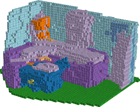
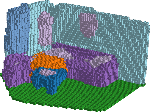
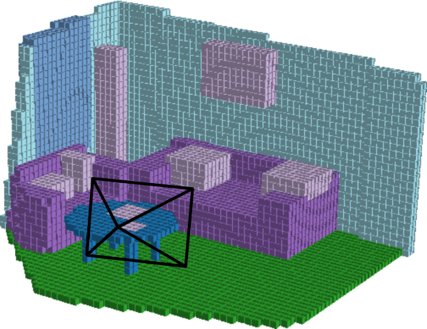
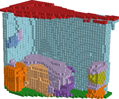
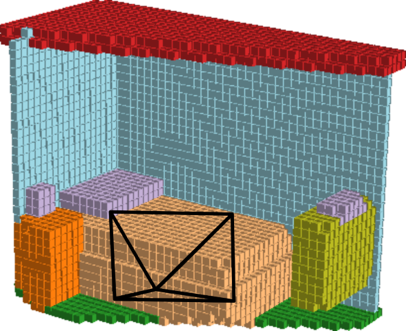
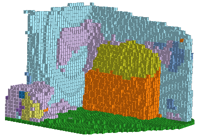
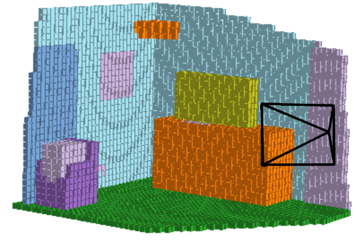
$\blacksquare$ceiling  $\blacksquare$floor  $\blacksquare$wall  $\blacksquare$window  $\blacksquare$chair  $\blacksquare$sofa  $\blacksquare$table  $\blacksquare$tvs  $\blacksquare$furniture  $\blacksquare$objects

(a) NYUv2[58] (test set).

Input	AICNet${}^{\text{rgb}}$ [39]	LMSCNet${}^{\text{rgb}}$ [55]	JS3CNet${}^{\text{rgb}}$ [69]	MonoScene (ours)	Ground Truth
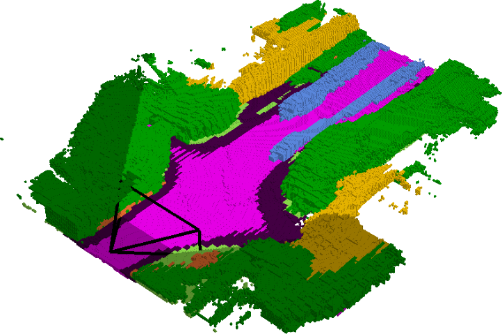
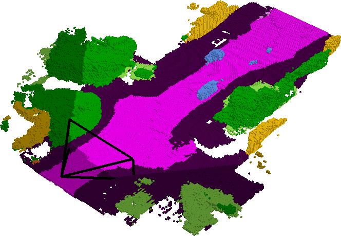
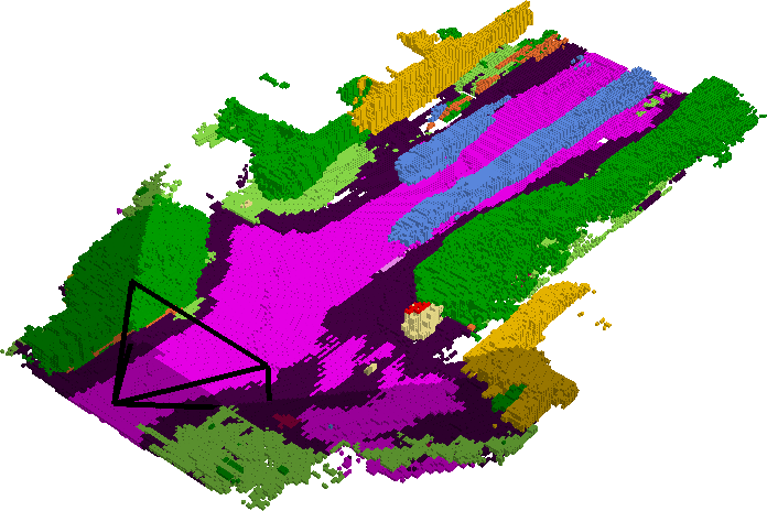
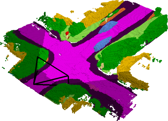
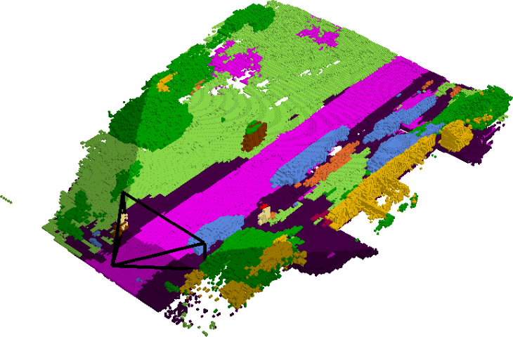
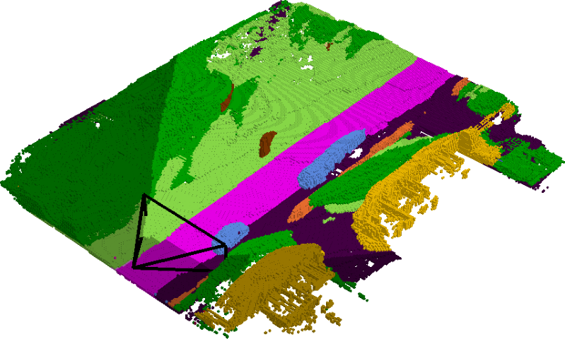
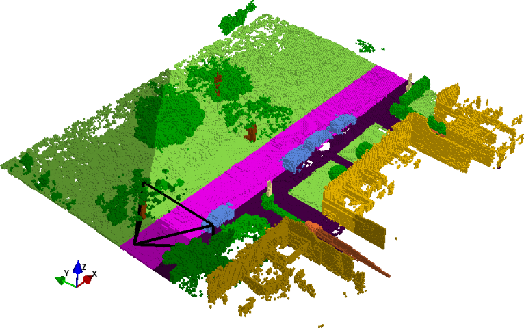
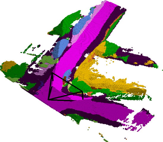
$\blacksquare$bicycle  $\blacksquare$car  $\blacksquare$motorcycle  $\blacksquare$truck  $\blacksquare$other vehicle  $\blacksquare$person  $\blacksquare$bicyclist  $\blacksquare$motorcyclist  $\blacksquare$road  $\blacksquare$parking
$\blacksquare$sidewalk  $\blacksquare$other ground  $\blacksquare$building  $\blacksquare$fence  $\blacksquare$vegetation  $\blacksquare$trunk  $\blacksquare$terrain  $\blacksquare$pole  $\blacksquare$traffic sign

(b) SemanticKITTI [3] (val set).

Figure 7: Outputs on 7(a) NYUv2 [58] and 7(b) SemanticKITTI [3]. In both, the input is shown left and the camera viewing frustum is shown in the ground truth (rightmost) with darker colors being parts of scenes unseen by the image in 7(b). MonoScene better captures the scene layout on both datasets. On indoor scene 7(a), it reconstructs thin objects like table legs (row 1), painting and tv (row 2), while in outdoor 7(b), it better estimates occluded geometry e.g. car (row 1–3) and better hallucinates the scenery beyond the field of view (row 1–4).

Qualitative. We compare our SSC outputs in Fig. 7 showing the input image (leftmost column) and its corresponding camera frustum in ground truth (rightmost). Notice the noisy labels in NYUv2 having missing objects (e.g. windows, rows 2; ceiling, row 3), and in SemanticKITTI having sparse geometry (e.g. holes in buildings, rows 1–3).

On indoor scenes (NYUv2, Fig. 7(a)), all methods correctly capture global scene layouts though only MonoScene recovers thin elements as table legs and cushions (row 1), or the painting frame and properly sized TV (row 2).

On complex cluttered outdoor scenes (SemanticKITTI, Fig. 7(b)), compared to baselines, MonoScene evidently captures better the scene layout, e.g. cross-roads (rows 1,3). It also infers finer occluded geometry which is apparent with cars in rows 1–3 having better shapes. Interestingly, despite a narrow camera field of view (FOV) with respect to the scene, MonoScene properly hallucinates scenery not imaged, i.e. outside of the camera FOV (darker voxels). This is striking in rows 3,4 where the bottom part of the scene is reasonably guessed, though not in the viewing frustum. Sec. B.1 provides in-/out-FOV performance details.

Method	Input	IoU	mIoU
2.5/3D
LMSCNet [55]	$x^{\text{occ}}$	44.1	20.4
AICNet [39]	$x^{\text{rgb}}$, $x^{\text{depth}}$	43.8	23.8
3DSketch [9]	$x^{\text{rgb}}$, $x^{\text{TSDF}}$	49.5	29.2
2D
MonoScene	$x^{\text{rgb}}$	42.5	26.9

(a) NYUv2 (test set)

Method	Input	IoU	mIoU
3D
LMSCNet [55]	$x^{\text{occ}}$	56.7	17.6
Local-DIFs [53]	$x^{\text{occ}}$	57.7	22.7
JS3C-Net [69]	$x^{\text{pts}}$	56.6	23.8
S3CNet [12]	$x^{\text{occ}}$	45.6	29.5
2D
MonoScene	$x^{\text{rgb}}$	34.2	11.1

(b) Sem.KITTI (hidden test set)

Table 3: 2.5/3D input baselines. Despite a single RGB, MonoScene still outperforms the mIoU of some indoor baselines.

4.2.2 Comparison against 2.5/3D-input baselines

For completeness, we also compare with some original baselines (i.e. using real 3D input) in Tab. 3. Despite the unfair setup since we use only RGB, in NYUv2 (Tab. 3(a)) we still beat the recent LMSCNet and AICNet in mIoU by a comfortable margin (+6.48 and +3.17), but with a lower IoU (-1.6 and -1.26). Of note AICNet also uses RGB in addition to depth, showing our method excels at recovering geometry from image only. 3DSketch, using RGB + TSDF, outperforms us on both mIoU and IoU showing the benefit of TSDF for SSC as mentioned in [56]. In SemanticKITTI (Tab. 3(b)), the baselines clearly surpass us in all metrics which relates both to the lidar-originated 3D input having a much wider horizontal FOV than the camera ($180^{\circ}$ vs $82^{\circ}$), and to the far more complex and cluttered outdoor scenes – thus harder to reconstruct from a single image viewpoint.

	NYUv2		SemanticKITTI
	IoU $\uparrow$	mIoU $\uparrow$	IoU $\uparrow$	mIoU $\uparrow$
Ours	42.51 $\pm$0.15	26.94 $\pm$0.10	37.12 $\pm$0.15	11.50 $\pm$0.14
Ours w/o FLoSP	28.39 $\pm$0.53	14.11 $\pm$0.21	27.55 $\pm$0.87	4.78$\pm$0.10
Ours w/o 3D CRP	41.39 $\pm$0.08	26.27 $\pm$0.15	36.20 $\pm$0.19	10.96 $\pm$0.21
Ours w/o $\mathcal{L}^{\text{sem}}_{\text{scal}}$	42.82 $\pm$0.22	25.33 $\pm$0.26	36.78 $\pm$0.34	9.89 $\pm$0.11
Ours w/o $\mathcal{L}^{\text{geo}}_{\text{scal}}$	40.96 $\pm$0.28	26.34 $\pm$0.23	34.92 $\pm$0.34	11.35 $\pm$0.22
Ours w/o $\mathcal{L}_{\text{fp}}$	41.90 $\pm$0.26	26.37 $\pm$0.16	36.74 $\pm$0.33	11.11 $\pm$0.24

Table 4: Architecture ablation. Our components boost performance on NYUv2 [58] (test set) and SemanticKitti [3] (val. set).

The large 2D – 2.5/3D gaps in Tab. 3 partly result of the low depth accuracy. For example, on NYUv2/Sem.KITTI AdaBins [4] gets 0.36/2.36m RMSE while voxels size is 0.08/0.2m. Furthermore, as we account for occluded voxels, our geometry is expectedly better. This is assessed using MonoScene geometry as input of LMSCNet, which improves IoU/mIoU on Sem.KITTI val. set from 28.61/6.70 to 35.94/9.44. Still, Tab. 4 shows that MonoScene predicts better geometry and semantics reaching 37.12/11.50.

4.3 Ablation studies

We ablate our MonoScene framework on both NYUv2 (test set) and SemanticKITTI (validation set), and report the average of 3 runs to account for training variability.

Architectural components. Tab. 4 shows that all components contribute to the best results. For ‘w/o FLoSP’, we instead interpolate and convolve the 2D decoder features to the required 3D UNet input size. Specifically, FLoSP (Sec. 3.1) is shown to be the most crucial as it improves remarkably both semantics ($[+12.83$,$+6.72]$ mIoU) and geometry ($[+14.11$,$+9.56]$ IoU). 3D CRP (Sec. 3.2) contributes equally to IoU (in $[+0.77$,$+1.12]$) and mIoU (in $[+0.54,+1.33]$). Both SCAL losses (Sec. 3.3.1) contribute differently as expected, since $\mathcal{L}^{\text{sem}}_{\text{scal}}$ helps semantics ($+1.61$ mIoU in both), while $\mathcal{L}^{\text{geo}}_{\text{scal}}$ boosts geometry ($[+1.55,+2.20]$ IoU). In NYUv2 only, $\mathcal{L}^{\text{sem}}_{\text{scal}}$ harms IoU (-0.31) but improves the same metric on SemanticKITTI (+0.34). Finally, the frustums proportion loss (Sec. 3.3.2) boosts both metrics on both datasets by at least $+0.38$ and up to $+0.61$.

2D scales  ($S$)	IoU $\uparrow$	mIoU $\uparrow$
$1,2,4,8$	42.51 $\pm$0.15	26.94 $\pm$0.10
$1,2,4$	42.08 $\pm$0.69	26.28 $\pm$0.24
$1,2$	41.56 $\pm$0.18	25.66 $\pm$0.21
$1$	41.57 $\pm$0.11	25.61 $\pm$0.43
w/o FLoSP	28.39 $\pm$0.53	14.11 $\pm$0.21

(a) Scales in FLoSP

$n$	$\mathcal{L}_{rel}$	IoU $\uparrow$	mIoU $\uparrow$
4	✓	42.51 $\pm$0.15	26.94 $\pm$0.10
	✗	42.24 $\pm$0.15	26.55 $\pm$0.29
2	✓	42.09 $\pm$0.15	26.63 $\pm$0.05
	✗	42.15 $\pm$0.26	26.47 $\pm$0.16
w/o 3D CRP		41.39 $\pm$0.08	26.27 $\pm$0.15

(b) Relations and supervision in 3D CRP

Table 5: Study of FLoSP and 3D CRP. 5(a) Projecting from different 2D scales ($S$) in FLoSP (Sec. 3.1) show more scales is better. 5(b) In our 3D CRP (Sec. 3.2) using more relations ($n$) and supervision ($\mathcal{L}_{rel}$) lead to higher metrics. Results are on NYUv2.

CoReNet
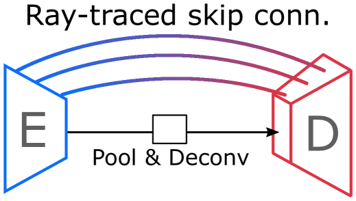
Ours-light

(a) Architectures (2D or 3D)

	IoU $\uparrow$	mIoU $\uparrow$
CoReNet (1,2,4)	30.60 $\pm$0.46	17.34 $\pm$0.37
Ours-light (1,2,4)	40.80 $\pm$0.43	25.90 $\pm$0.63
Ours-light (1)	40.13 $\pm$0.31	25.33 $\pm$0.58

(b) Performance

Figure 8: Type of 2D-3D features projections. 8(a) Comparing our FLoSP and ‘Ray-traced skip connections’ from CoReNet [52] (cf. text) shows in 8(b) we get significantly better results at comparable (1,2,4) scales or even with only one (1).

Effect of features projection. We now study in-depth the effect of FLoSP (Sec. 3.1) at the core our RGB-based task. In Tab. 5(a), we use our FLoSP projecting only 2D features from given 2D scales by changing $S$ in Eq. 1. More 2D scales boosts IoU and mIoU consistently and leans to lower variance – showing (1,2,4,8) projections are indeed best.

We further compare FLoSP to the ‘Ray-traced skip connections’ of CoReNet [52] being close in nature, putting our best effort to push CoReNet performance. To properly evaluate only the effect of features projection, we remove our other components, producing a light version (‘Ours-light’) with the same 2D encoder (E), 3D decoder (D), and projection scales (1,2,4), corresponding to all possible scales in the 3D decoder, as in CoReNet, shown in Fig. 8(a). On NYUv2, Fig. 8(b) shows FLoSP is very significantly better (+10.2 IoU, +8.56 mIoU). We conjecture this relates to the fact that CoReNet applies same-scale 2D-3D connections, while FLoSP disentangles 2D-3D scales, letting the network relies on self-learned relevant features, confirmed by the good performance of the (1) scale in Fig. 8(b).

Effect of relations in 3D CRP. While 3D CRP (Sec. 3.2) is shown beneficial in Tab. 4, we evaluate the effect of different numbers of relations (i.e. $n$). Tab. 5(b) shows the benefit of our 4 relations $\mathcal{M}{=}\{\textbf{f}_{\textbf{s}},\textbf{f}_{\textbf{d}},\textbf{o}_{\textbf{s}},\textbf{o}_{\textbf{d}}\}$ instead of only 2 (i.e. $\mathcal{M}{=}\{\textbf{s},\textbf{d}\}$), which matches our expectation due to the overwhelming imbalance of free/occupied voxels ($\approx{}9{:}1$ in NYUv2). Our supervision of relation matrices $\hat{A}$ with the relation loss $\mathcal{L}_{rel}$ from Eq. 3 also shows an increase of all metrics. Without supervision, our 3D CRP acts as a self-attention layer that learns the context information implicitly.

	NYUv2		SemanticKITTI
$\ell{\times}\ell$	IoU $\uparrow$	mIoU $\uparrow$	IoU $\uparrow$	mIoU $\uparrow$
$8\times 8$	42.51 $\pm$0.15	26.94 $\pm$0.10	37.12 $\pm$0.15	11.50 $\pm$0.14
$4\times 4$	42.52 $\pm$0.12	26.85 $\pm$0.19	37.09 $\pm$0.09	11.45 $\pm$0.15
$2\times 2$	42.41 $\pm$0.13	26.85 $\pm$0.22	36.88 $\pm$0.11	11.27 $\pm$0.25
$1\times 1$	42.39 $\pm$0.18	26.52 $\pm$0.31	36.83 $\pm$0.42	11.33 $\pm$0.11
w/o $\mathcal{L}_{\text{fp}}$	41.90 $\pm$0.26	26.37 $\pm$0.16	36.74 $\pm$0.33	11.11 $\pm$0.24

Table 6: Frustums Proportion loss ablation. Varying the number of local frustums ($\ell{\times}\ell$) in our loss shows more frustums (i.e. smaller) lead to finer guidance and better results on both datasets.

Effect of local frustums loss. Tab. 6 shows the effect of varying number of $\ell{\times}\ell$ frustums (Eq. 8, Sec. 3.3.2) on both datasets. Higher numbers result in smaller frustums, i.e. finer local supervision. As $\ell{\times}\ell$ increases, all metrics increase accordingly, showing the loss benefit, especially when compared to applied image-wise (i.e. $1{\times}1$).

Cityscapes [17]	Nuscenes [5]	SemanticKITTI [3]	KITTI-360 [44]
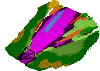
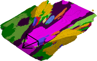
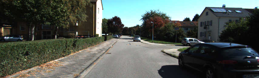
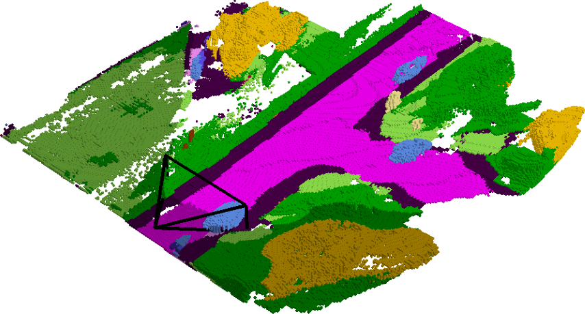
r0cmb0pt	r0cmb0pt	r0cmb0pt	r0cmb0pt
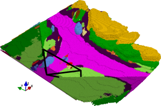
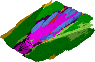
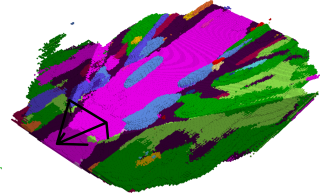
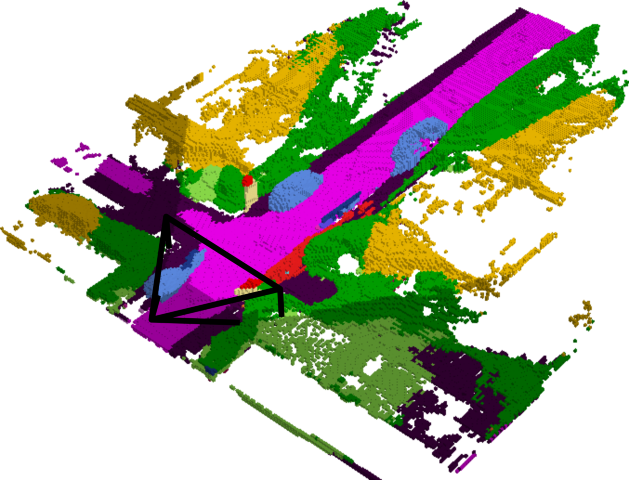
r0cmb0pt	r0cmb0pt	r0cmb0pt	r0cmb0pt
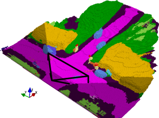
(49∘, 25∘)	(65∘, 39∘)	(H=82∘, V=29∘)	(104∘, 38∘)

Figure 9: Camera effects. Outputs of MonoScene when trained on Sem.KITTI having horizontal FOV of 82^∘, and tested on datasets with decreasing (left) or increasing (right) FOV.

5 Discussion

MonoScene tackles monocular SSC originally using successive 2D-3D UNets, bridged by a new features projection, with increased contextual awareness and new losses.

Limitations. Despite good results, our framework still struggles to infer fine-grained geometry, or to separate semantically-similar classes, e.g. car/truck or chair/sofa. It also performs poorly on small objects partly due to their scarcity (${<}0.3\%$ in Sem.KITTI [3]). Due to the single viewpoint, occlusion artefacts such as distortions are visible along the line of sight in outdoor scenes. Additionally, as we exploit 2D-3D projection with the FLoSP module (Sec. 3.1), we evaluate the effect of inferring from datasets having various camera setups, showing in Fig. 9 that results – though consistent – have increasingly greater distortion when departing from the camera settings of the training set.

Broader impact, Ethics. Jointly understanding the 3D geometry and semantics from image paves ways for better mixed reality, photo editing or mobile robotics applications. But the inevitable errors in the scene understanding could have fatal issues (e.g. autonomous driving) and such algorithms should always be seconded by other means. Acknowledgment This work used HPC resources from GENCI–IDRIS (Grant 2021-AD011012808). It was done in the SAMBA collaborative project, co-funded by BpiFrance in the Investissement d’Avenir Program.

We provide details about the main baselines and MonoScene in Appendix A, and include additional qualitative and quantitative results in Appendix B.

Results on image sequences are in the supplementary video: https://youtu.be/qh7La1tRJmE.

Appendix A Architectures details

A.1 Baselines

AICNet [39].

We use the official implementation of AICNet. For the RGB-inferred version, i.e. AICNet${}^{\text{rgb}}$, we infer depth with the pre-trained AdaBins [4] on NYUv2 [58] and SemanticKITTI [3] from the official repository.

3DSketch [9].

We use 3DSketch official code. For 3DSketch${}^{\text{rgb}}$, we again use AdaBins (cf. above) and convert depth to TSDF with ‘tsdf-fusion’ from the 3DMatch Toolbox [74].

JS3C-Net [69].

We use the official code of JS3C-Net. For JS3C-Net${}^{\text{rgb}}$, we generate the input point cloud by unprojecting the predicted depth (using AdaBins) to 3D using the camera intrinsics. The semantic point clouds, required to train JS3C-Net, are obtained by augmenting the unprojected point clouds with the 2D semantics obtained using the code of [82].

LMSCNet [55].

We use the official implementation of LMSCNet. For LMSCNet${}^{\text{rgb}}$, the input occupancy grid is obtained by discretizing the unprojected point cloud.

A.2 MonoScene

Fig. 10 details our 3D UNet. Similar to 3DSketch [9], we adopt DDR [40] as the basic building block for large receptive field and low memory cost. The 3D encoder has 2 layers, each downscales by half and has 4 DDR blocks. The 3D decoder has two deconv layers, each doubles the scale. Similar to others [55] the completion head has an ASPP with dilations (1, 2, 3) to gather multi-scale features and an optional deconv to reach output size – used in SemanticKITTI only.

For training, MonoScene took 7 hours using 2 V100 32g GPUs (2 items per GPU) on NYUv2 [58] and 28 hours to train using 4 V100 32g GPUs (1 item per GPU) on SemanticKITTI [3].

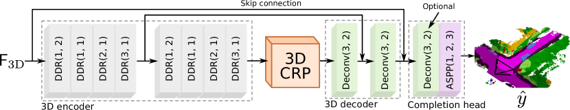
Figure 10: MonoScene 3D network. The 3D UNet uses 2 downscale layers with DDR blocks [40] and 2 upscale layers with deconv. The completion head uses ASPP and an optional deconv layer. Notations: DDR(dilation, downsample rate), Deconv(kernel size, dilation), ASPP(dilations).

		SC	SSC
Method	SSC Input	IoU	$\blacksquare$ road (15.30%)	$\blacksquare$ sidewalk (11.13%)	$\blacksquare$ parking (1.12%)	$\blacksquare$ other-ground (0.56%)	$\blacksquare$ building (14.1%)	$\blacksquare$ car (3.92%)	$\blacksquare$ truck (0.16%)	$\blacksquare$ bicycle (0.03%)	$\blacksquare$ motorcycle (0.03%)	$\blacksquare$ other-vehicle (0.20%)	$\blacksquare$ vegetation (39.3%)	$\blacksquare$ trunk (0.51%)	$\blacksquare$ terrain (9.17%)	$\blacksquare$ person (0.07%)	$\blacksquare$ bicyclist (0.07%)	$\blacksquare$ motorcyclist (0.05%)	$\blacksquare$ fence (3.90%)	$\blacksquare$ pole (0.29%)	$\blacksquare$ traffic-sign (0.08%)	mIoU
LMSCNet${}^{\text{rgb}}$ [55]	$\hat{x}^{\text{occ}}_{\text{3D}}$	28.61	40.68	18.22	4.38	0.00	10.31	18.33	0.00	0.00	0.00	0.00	13.66	0.02	20.54	0.00	0.00	0.00	1.21	0.00	0.00	6.70
3DSketch${}^{\text{rgb}}$ [9]	$x^{\text{rgb}}$,$\hat{x}^{\text{TSDF}}$	33.30	41.32	21.63	0.00	0.00	14.81	18.59	0.00	0.00	0.00	0.00	19.09	0.00	26.40	0.00	0.00	0.00	0.73	0.00	0.00	7.50
AICNet${}^{\text{rgb}}$ [39]	$x^{\text{rgb}}$,$\hat{x}^{\text{depth}}$	29.59	43.55	20.55	11.97	0.07	12.94	14.71	4.53	0.00	0.00	0.00	15.37	2.90	28.71	0.00	0.00	0.00	2.52	0.06	0.00	8.31
JS3C-Net${}^{\text{rgb}}$ [69]	$\hat{x}^{\text{pts}}$	38.98	50.49	23.74	11.94	0.07	15.03	24.65	4.41	0.00	0.00	6.15	18.11	4.33	26.86	0.67	0.27	0.00	3.94	3.77	1.45	10.31
MonoScene (ours)	$x^{\text{rgb}}$	37.12	57.47	27.05	15.72	0.87	14.24	23.55	7.83	0.20	0.77	3.59	18.12	2.57	30.76	1.79	1.03	0.00	6.39	4.11	2.48	11.50

* Uses pretrained semantic segmentation network.

Table 7: Performance on SemanticKITTI [3] (validation set). We report the performance on semantic scene completion (SSC - mIoU) and scene completion (SC - IoU) for RGB-inferred baselines and our method.

Appendix B Additional results

B.1 SemanticKITTI

Quantitative performance.

We report performance on validation set in Tab. 7. Comparing against the test set performance from the main paper Tab. 1b, we notice MonoScene generalizes better than JS3C-Net${}^{\text{rgb}}$ and AICNet${}^{\text{rgb}}$ since the validation and test set gap is smaller (${-}0.42$ vs ${-}1.34$ and ${-}1.22$). We also report the complete SemanticKITTI official benchmark (i.e. hidden test set) in Tab. 8 showing that while MonoScene uses only RGB, it still outperforms some of the 3D input SSC baselines.

Method	Input	IoU	mIoU
3D
SSCNet [59]	$x^{\text{TSDF}}$	29.8	9.5
TS3D [25]	$x^{\text{TSDF}}{+}x^{\text{rgb}}$	29.8	9.5
TS3D+DNet [3]	$x^{\text{TSDF}}{+}x^{\text{rgb}}$	25.0	10.2
ESSCNet [77]	$x^{\text{pts}}$	41.8	17.5
LMSCNet [55]	$x^{\text{occ}}$	56.7	17.6
TS3D+DNet+SATNet [3]	$x^{\text{occ}}$	50.6	17.7
Local-DIFs [53]	$x^{\text{occ}}$	57.7	22.7
JS3C-Net [69]	$x^{\text{pts}}$	56.6	23.8
S3CNet [12]	$x^{\text{occ}}$	45.6	29.5
2D
MonoScene	$x^{\text{rgb}}$	34.2	11.1

Table 8: Complete SemanticKITTI official benchmark (hidden test set). Results are taken from [56]. Despite using only single RGB image as input, MonoScene still surpasses some of the SSC baselines with 3D input.

Input	AICNet${}^{\text{rgb}}$ [39]	LMSCNet${}^{\text{rgb}}$ [55]	JS3CNet${}^{\text{rgb}}$ [69]	MonoScene (ours)	Ground Truth
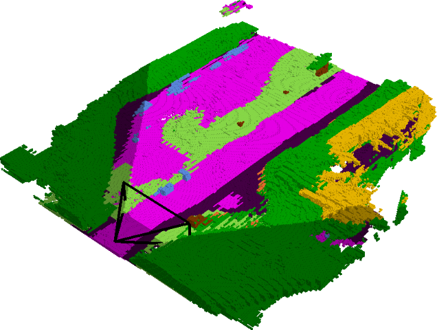
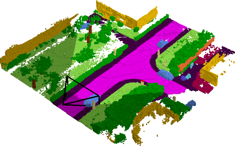
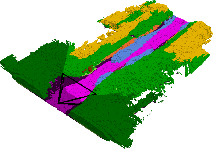
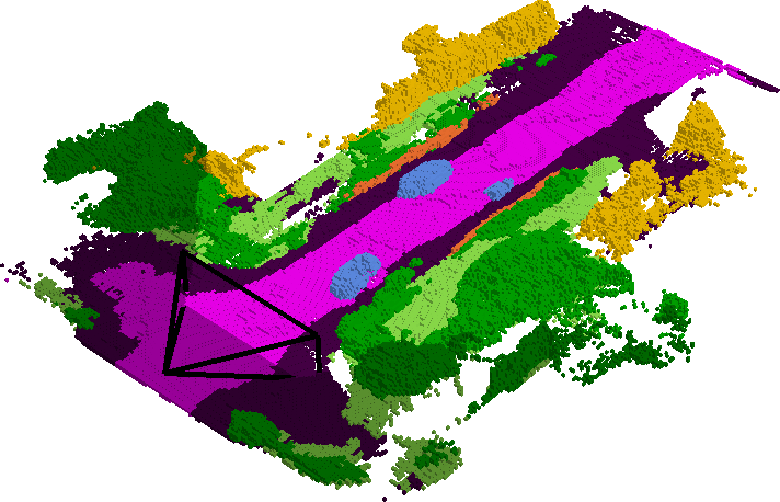
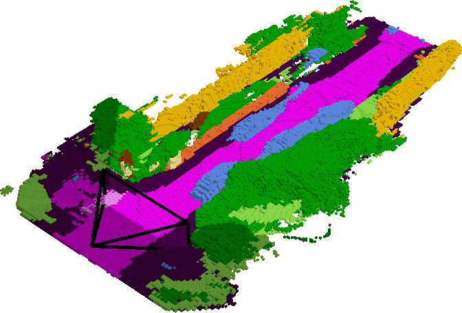
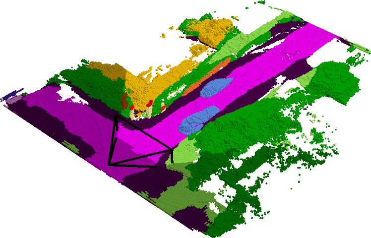
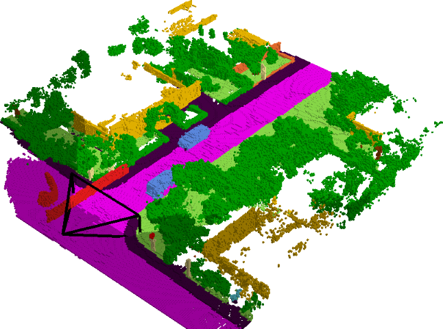
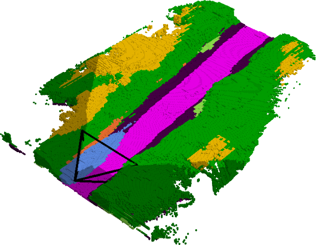
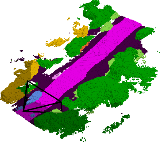
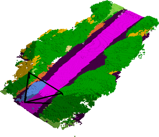
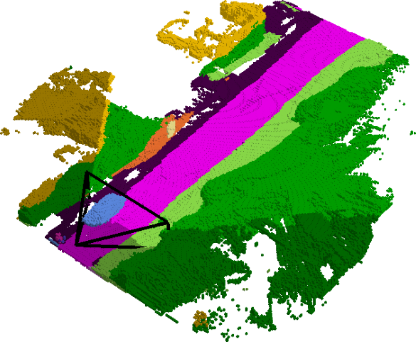
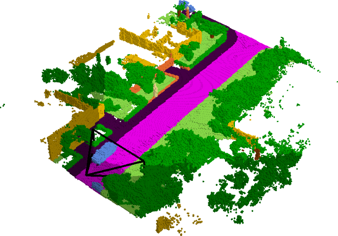
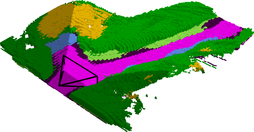
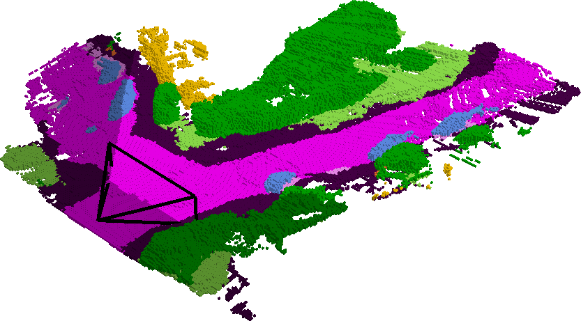
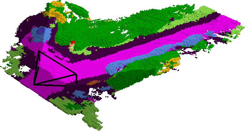
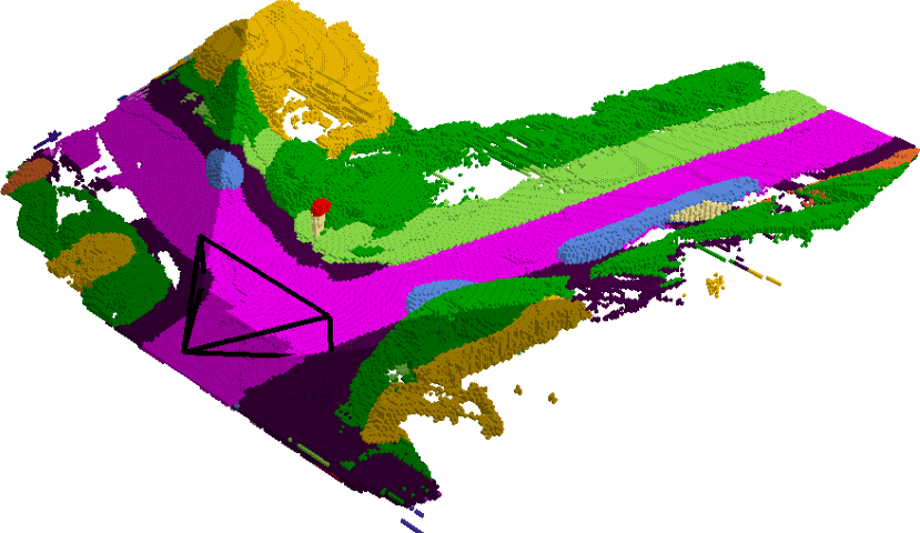
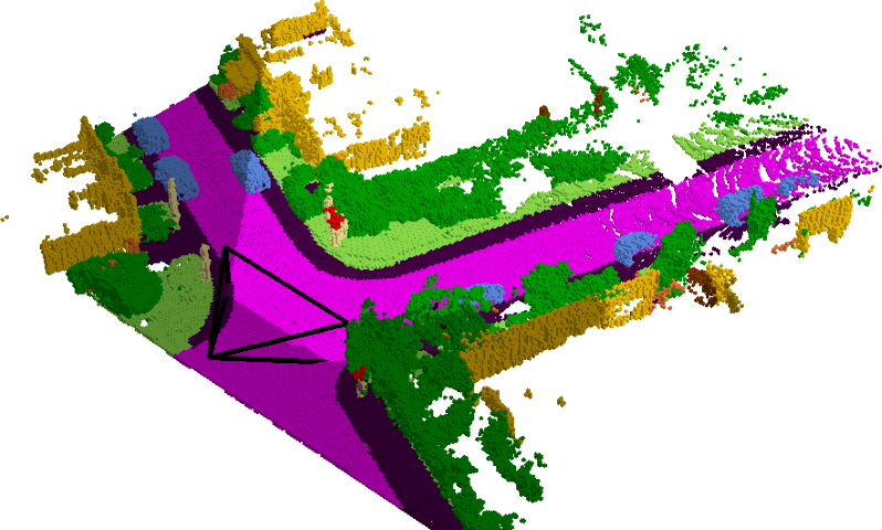
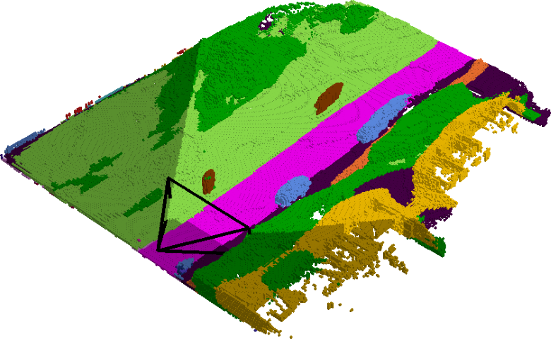
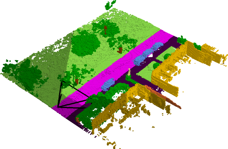
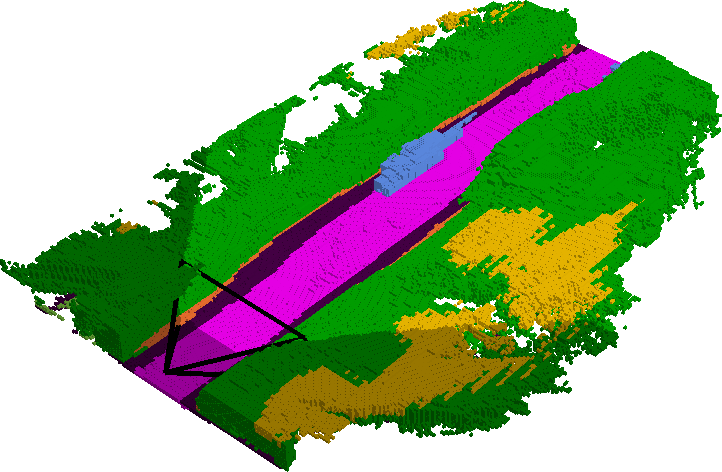
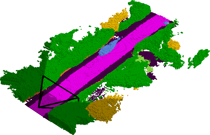
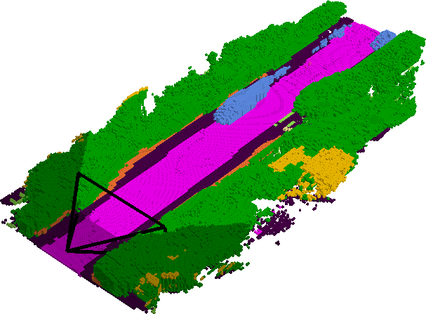
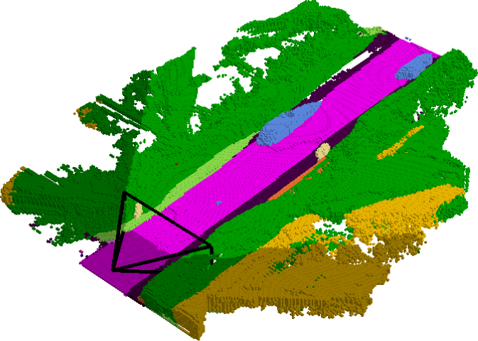
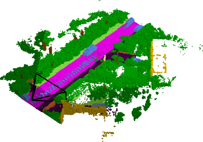
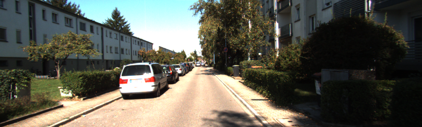
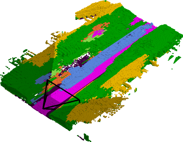
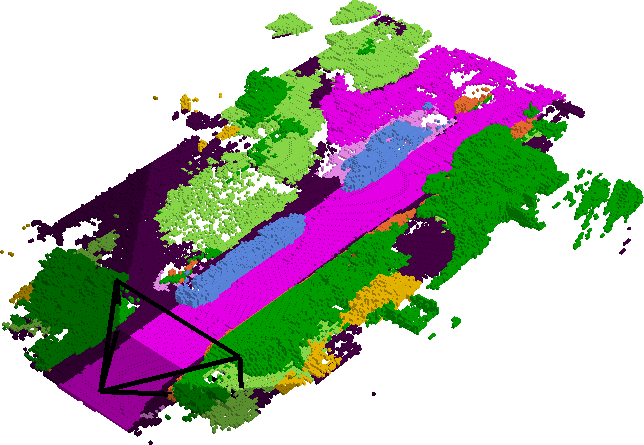
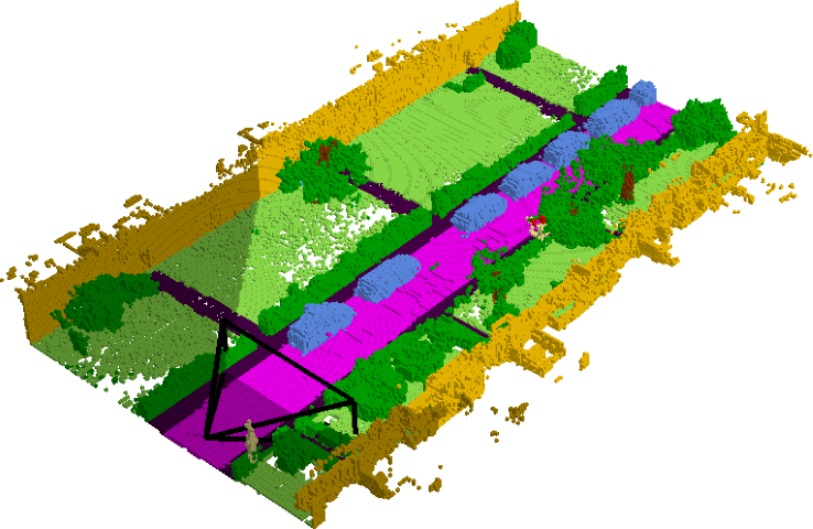
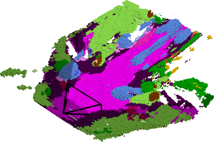
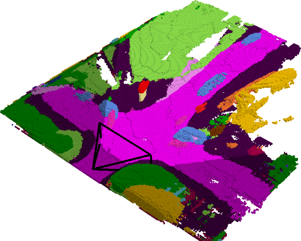
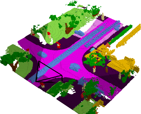
$\blacksquare$bicycle  $\blacksquare$car  $\blacksquare$motorcycle  $\blacksquare$truck  $\blacksquare$other vehicle  $\blacksquare$person  $\blacksquare$bicyclist  $\blacksquare$motorcyclist  $\blacksquare$road  $\blacksquare$parking
$\blacksquare$sidewalk  $\blacksquare$other ground  $\blacksquare$building  $\blacksquare$fence  $\blacksquare$vegetation  $\blacksquare$trunk  $\blacksquare$terrain  $\blacksquare$pole  $\blacksquare$traffic sign

Figure 11: Results on SemanticKITTI [3] (validation set). The input is shown left. Darker voxels represent the scenery outside the viewing frustum (i.e. unseen by the image).

Qualitative performance.

In Fig. 11 we also include additional qualitative results. Compared to all baselines, MonoScene captures better landscape and objects (e.g. cars, rows 3-9; pedestrian, rows 6, 10; traffic-sign, rows 3, 5). Still, it struggles to predict thin small objects (e.g. trunk, row 1; pedestrian, row 3; traffic-sign, row 2, 6), separate far away consecutive cars (e.g. row 5, 7, 8), and infer very complex, highly cluttered scenes (e.g. rows 9, 10).

Evaluation scope.

Tab. 9 reports the performance when considering either only the voxels inside FOV (in-FOV), outside FOV (out-FOV), or all voxels (Whole Scene) as reported in the main paper. Compared to the Whole Scene, the in-FOV performance is higher since it considers visible surfaces, whereas the out-FOV performance is significantly lower since the image does not observe it.

	in-FOV		out-FOV		Whole Scene
	IoU $\uparrow$	mIoU $\uparrow$	IoU $\uparrow$	mIoU $\uparrow$	IoU $\uparrow$	mIoU $\uparrow$
LMSCNet${}^{\text{rgb}}$ [55]	37.62	8.87	25.36	5.48	34.41	8.17
3DSketch${}^{\text{rgb}}$ [9]	32.24	7.82	26.50	5.83	33.30	7.50
AICNet${}^{\text{rgb}}$ [39]	35.69	8.75	25.79	5.61	29.59	8.31
JS3C-Net${}^{\text{rgb}}$ [69]	42.22	11.29	28.27	6.31	38.98	10.31
MonoScene(ours)	39.13	12.78	31.60	7.45	37.12	11.50

* Uses pretrained semantic segmentation network.

Table 9: SemanticKITTI performance (validation set) on in-/out-FOV and the Whole Scene. We report the performance on the scenery inside (in-FOV), outside (out-FOV) camera FOV, and considering all voxels (Whole Scene). MonoScene is best in most cases, with in-FOV performance logically higher.

B.2 NYUv2

We show additional qualitative results in Fig. 12. In overall, MonoScene predicts better scene layouts and better objects geometry, evidently in rows 1-4, 6, 9, 10. Still, MonoScene mispredicts complex (e.g. bookshelfs, row 1, 4, 6), or rare objects (running machine, row 8). Sometimes, it confuses semantically-similar classes (e.g. window/objects, row 6, 8; beds/objects, row 1, 5; furniture/table, row 1, 2) due to the high variance of indoor scene i.e. wide range of camera poses, objects have completely different appearances, poses and positions even in the same category e.g. beds (rows 1, 5-7, 9); sofa (row 2-4).

Input	LMSCNet${}^{\text{rgb}}$ [55]	AICNet${}^{\text{rgb}}$ [39]	3DSketch${}^{\text{rgb}}$ [9]	MonoScene (ours)	Ground Truth
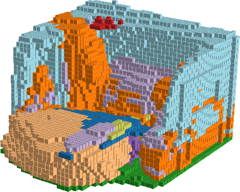
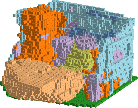
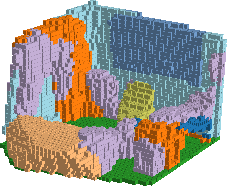
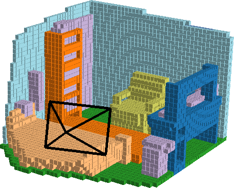
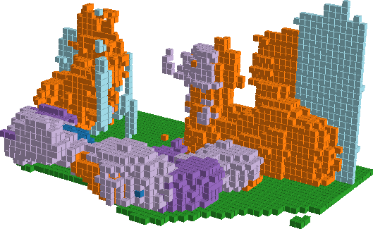
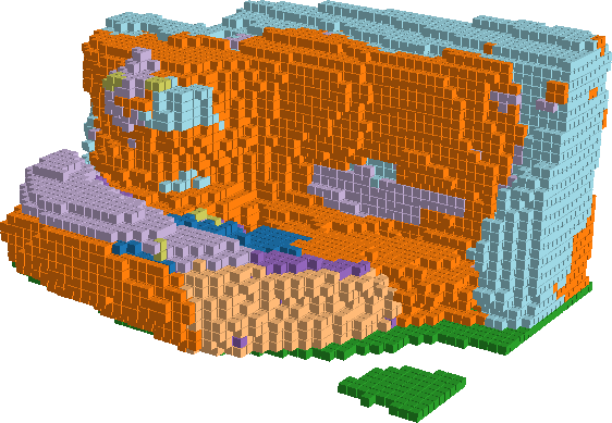
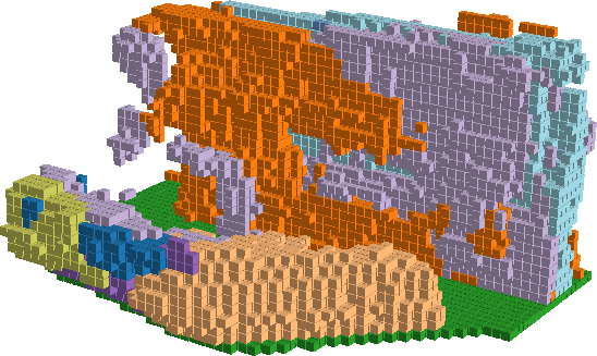
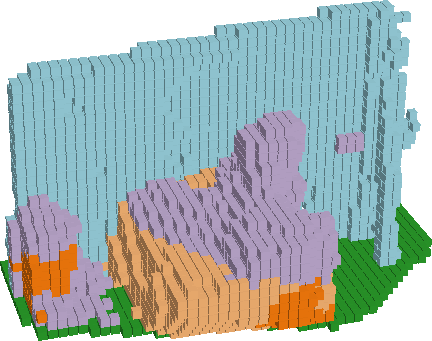
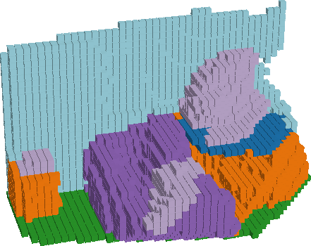
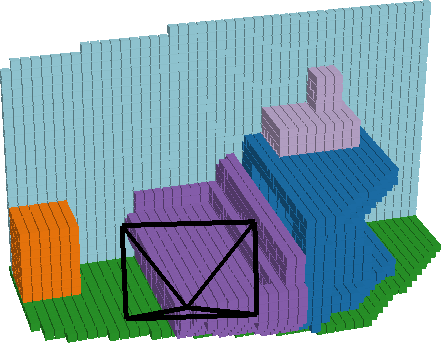
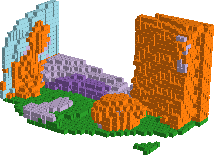
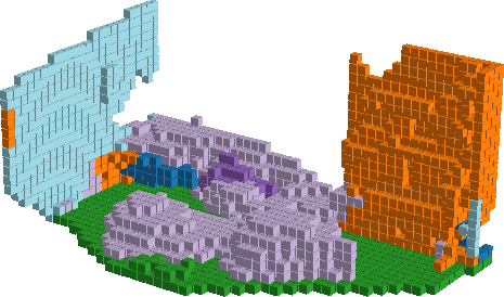
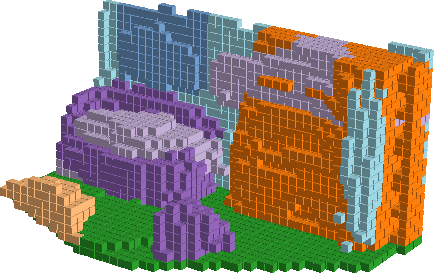
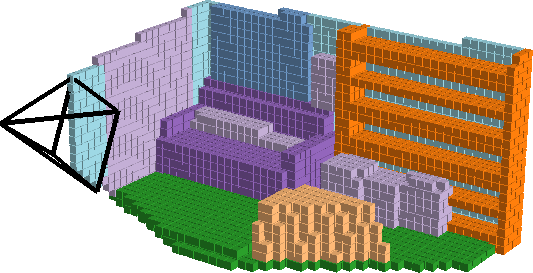
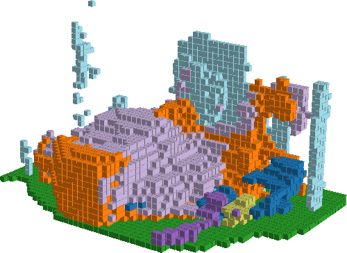
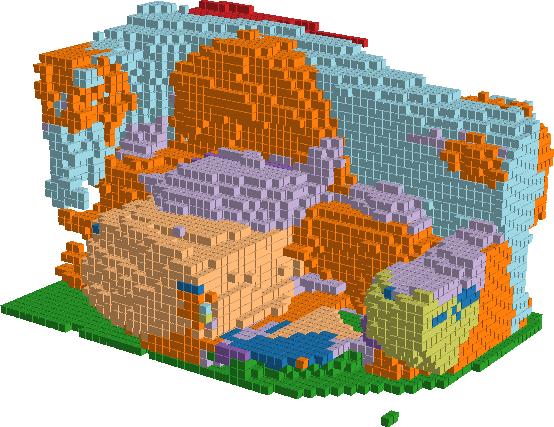
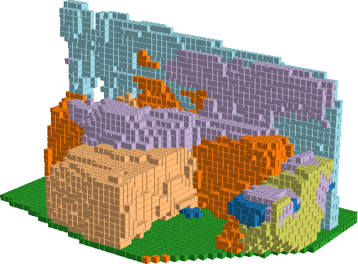
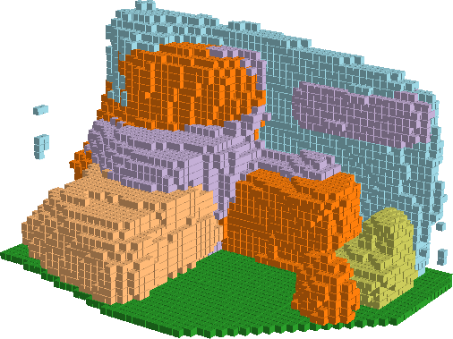
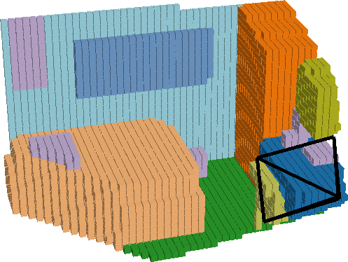
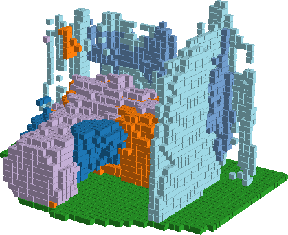
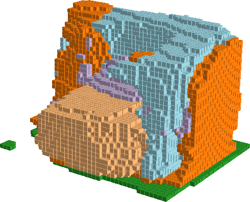
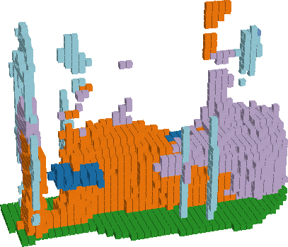
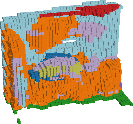
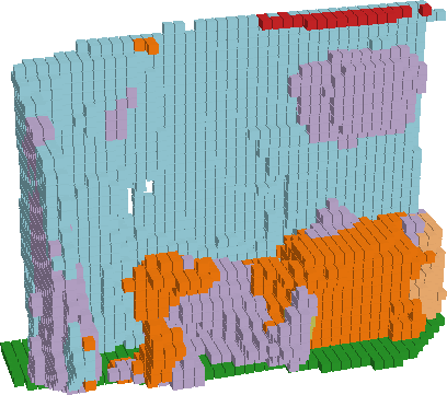
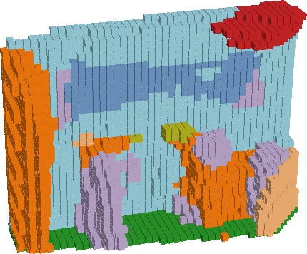
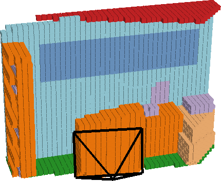
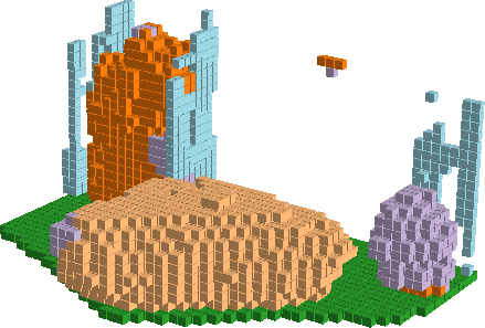
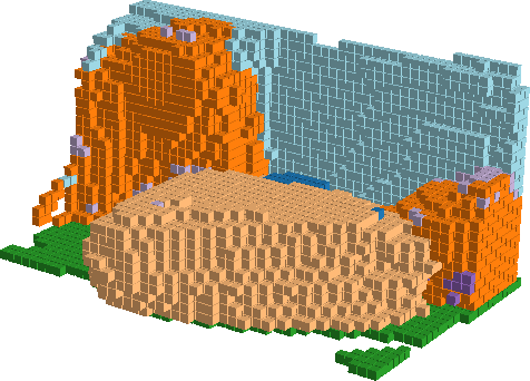
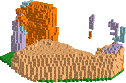
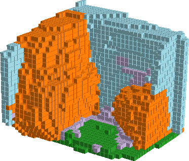
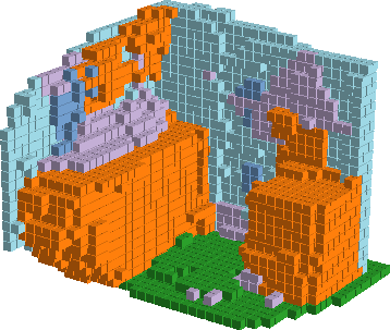
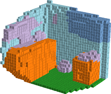
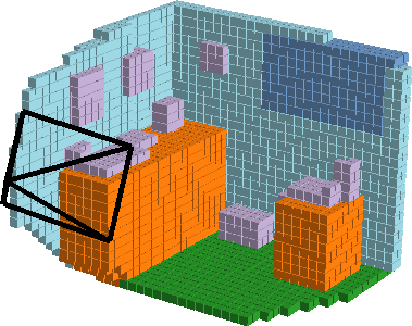
$\blacksquare$ceiling  $\blacksquare$floor  $\blacksquare$wall  $\blacksquare$window  $\blacksquare$chair  $\blacksquare$sofa  $\blacksquare$table  $\blacksquare$tvs  $\blacksquare$furniture  $\blacksquare$objects

Figure 12: Results on NYUv2[58] (test set). The input is shown leftmost and the camera viewing frustum is shown in the ground truth (rightmost).

B.3 Generalization

Fig. 13 illustrates the predictions of MonoScene, trained on SemanticKITTI, on datasets with different camera setups. We can see the increase in distortion as the camera setups depart from the ones used during training. Furthermore, the domain gap (i.e. city, country, etc.) also plays an important role. As MonoScene is trained on the mid-size German city of Karlsruhe, with residential scenes and narrow roads, the gap is smaller with KITTI-360 having similar scenes. The results on nuScenes and Cityscapes suffer both from the camera setup changes and the large metropolitan scenes (i.e. Stuttgart - Cityscapes; Singapore, Boston - nuScenes) having wider streets.

Cityscapes [17]	nuScenes [5]	SemanticKITTI [3]	KITTI-360 [44]
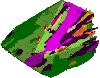
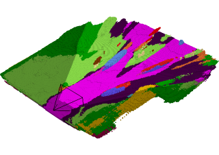
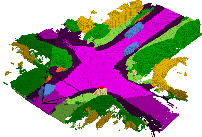
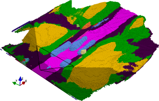
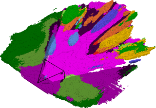
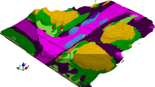
r0cmb0pt	r0cmb0pt	r0cmb0pt	r0cmb0pt
r0cmb0pt	r0cmb0pt	r0cmb0pt	r0cmb0pt
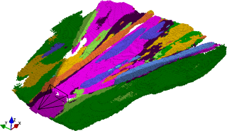
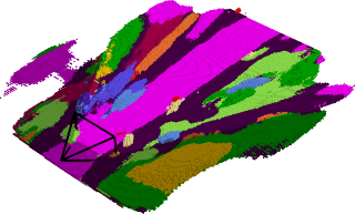
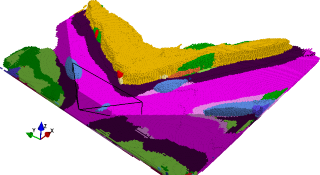
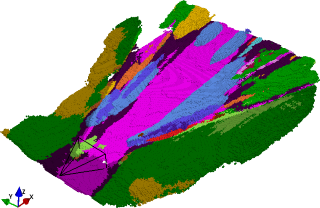
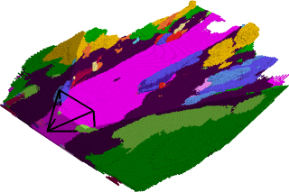
r0cmb0pt	r0cmb0pt	r0cmb0pt	r0cmb0pt
r0cmb0pt	r0cmb0pt	r0cmb0pt	r0cmb0pt
r0cmb0pt	r0cmb0pt	r0cmb0pt	r0cmb0pt
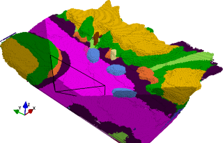
(49∘, 25∘)	(65∘, 39∘)	(H=82∘, V=29∘)	(104∘, 38∘)

Figure 13: Domain gap and Camera effects. Outputs of MonoScene when trained on SemanticKITTI having horizontal FOV of 82^∘, and tested on datasets with decreasing (left) or increasing (right) FOV. SemanticKITTI and KITTI-360 are recored in mid-size German city of Karlsruhe while nuScenes and Cityscapes are from large metropolitan areas (e.g. Stuttgart - Cityscapes; Singapore, Boston - nuScenes) whose streets are much wider, denser and have different landscapes.

References

- [1] Panos Achlioptas, Olga Diamanti, Ioannis Mitliagkas, and Leonidas Guibas. Learning representations and generative models for 3D point clouds. In ICML, 2018.
- [2] Armen Avetisyan, Manuel Dahnert, Angela Dai, Manolis Savva, Angel X. Chang, and Matthias Niessner. Scan2cad: Learning cad model alignment in rgb-d scans. In CVPR, 2019.
- [3] J. Behley, M. Garbade, A. Milioto, J. Quenzel, S. Behnke, C. Stachniss, and J. Gall. SemanticKITTI: A Dataset for Semantic Scene Understanding of LiDAR Sequences. In ICCV, 2019.
- [4] Shariq Farooq Bhat, Ibraheem Alhashim, and Peter Wonka. AdaBins: Depth Estimation using Adaptive Bins. In CVPR, 2021.
- [5] Holger Caesar, Varun Bankiti, Alex H. Lang, Sourabh Vora, Venice Erin Liong, Qiang Xu, Anush Krishnan, Yu Pan, Giancarlo Baldan, and Oscar Beijbom. nuscenes: A multimodal dataset for autonomous driving. In CVPR, 2020.
- [6] Yingjie Cai, Xuesong Chen, Chao Zhang, Kwan-Yee Lin, Xiaogang Wang, and Hongsheng Li. Semantic scene completion via integrating instances and scene in-the-loop. In CVPR, 2021.
- [7] Liang-Chieh Chen, George Papandreou, Iasonas Kokkinos, Kevin P. Murphy, and Alan Loddon Yuille. Deeplab: Semantic image segmentation with deep convolutional nets, atrous convolution, and fully connected crfs. T-PAMI, 2018.
- [8] R. Chen, Zhiyong Huang, and Yuanlong Yu. Am2fnet: Attention-based multiscale & multi-modality fused network. ROBIO, 2019.
- [9] Xiaokang Chen, Kwan-Yee Lin, Chen Qian, Gang Zeng, and Hongsheng Li. 3d sketch-aware semantic scene completion via semi-supervised structure prior. In CVPR, 2020.
- [10] Yueh-Tung Chen, Martin Garbade, and Juergen Gall. 3d semantic scene completion from a single depth image using adversarial training. In ICIP, 2019.
- [11] Zhiqin Chen, Andrea Tagliasacchi, and Hao Zhang. Bsp-net: Generating compact meshes via binary space partitioning. In CVPR, 2020.
- [12] Ran Cheng, Christopher Agia, Yuan Ren, Xinhai Li, and Bingbing Liu. S3cnet: A sparse semantic scene completion network for lidar point clouds. In CoRL, 2020.
- [13] Shun cheng Wu, Keisuke Tateno, Nassir Navab, and Federico Tombari. Scfusion: Real-time incremental scene reconstruction with semantic completion. In 3DV, 2020.
- [14] Ian Cherabier, Johannes L. Schönberger, M. Oswald, M. Pollefeys, and Andreas Geiger. Learning priors for semantic 3D reconstruction. In ECCV, 2018.
- [15] Jaesung Choe, Sunghoon Im, François Rameau, Minjun Kang, and In-So Kweon. Volumefusion: Deep depth fusion for 3d scene reconstruction. In ICCV, 2021.
- [16] Christopher B. Choy, Danfei Xu, JunYoung Gwak, Kevin Chen, and Silvio Savarese. 3d-r2n2: A unified approach for single and multi-view 3d object reconstruction. In ECCV, 2016.
- [17] Marius Cordts, Mohamed Omran, Sebastian Ramos, Timo Rehfeld, Markus Enzweiler, Rodrigo Benenson, Uwe Franke, Stefan Roth, and Bernt Schiele. The cityscapes dataset for semantic urban scene understanding. In CVPR, 2016.
- [18] Manuel Dahnert, Ji Hou, Matthias Nießner, and Angela Dai. Panoptic 3d scene reconstruction from a single rgb image. In NeurIPS, 2021.
- [19] Angela Dai, Christian Diller, and Matthias Nießner. Sg-nn: Sparse generative neural networks for self-supervised scene completion of rgb-d scans. In CVPR, 2020.
- [20] Aloisio Dourado, Teofilo E. de Campos, Hansung Kim, and Adrian Hilton. EdgeNet: Semantic scene completion from a single RGB-D image. In ICPR, 2020.
- [21] A. Dourado, H. Kim, T. de Campos, and A. Hilton. Semantic scene completion from a single 360-degree image and depth map. In VISAPP, 2020.
- [22] George Fahim, Khalid Amin, and Sameh Zarif. Single-View 3D reconstruction: A Survey of deep learning methods. Computers & Graphics, 2021.
- [23] Haoqiang Fan, Hao Su, and Leonidas J. Guibas. A point set generation network for 3d object reconstruction from a single image. In CVPR, 2017.
- [24] Jun Fu, Jing Liu, Haijie Tian, Yong Li, Yongjun Bao, Zhiwei Fang, and Hanqing Lu. Dual attention network for scene segmentation. In CVPR, 2019.
- [25] Martin Garbade, Johann Sawatzky, Alexander Richard, and Juergen Gall. Two stream 3d semantic scene completion. In CVPRW, 2019.
- [26] Rohit Girdhar, David F. Fouhey, Mikel Rodriguez, and Abhinav Gupta. Learning a predictable and generative vector representation for objects. In ECCV, 2016.
- [27] Georgia Gkioxari, Jitendra Malik, and Justin Johnson. Mesh r-cnn. In ICCV, 2019.
- [28] Alexander Grabner, Peter M Roth, and Vincent Lepetit. Location field descriptors: Single image 3d model retrieval in the wild. In 3DV, 2019.
- [29] Andre Bernardes Soares Guedes, Teófilo Emídio de Campos, and Adrian Hilton. Semantic scene completion combining colour and depth: preliminary experiments. ArXiv, abs/1802.04735, 2018.
- [30] Xian-Feng Han, Hamid Laga, and Mohammed Bennamoun. Image-based 3d object reconstruction: State-of-the-art and trends in the deep learning era. T-PAMI, 2019.
- [31] Derek Hoiem, Alexei A Efros, and Martial Hebert. Geometric context from a single image. In ICCV, 2005.
- [32] Siyuan Huang, Siyuan Qi, Yixin Zhu, Yinxue Xiao, Yuanlu Xu, and Song-Chun Zhu. Holistic 3d scene parsing and reconstruction from a single rgb image. In ECCV, 2018.
- [33] Zilong Huang, Xinggang Wang, Yunchao Wei, Lichao Huang, Humphrey Shi, Wenyu Liu, and Thomas S. Huang. Ccnet: Criss-cross attention for semantic segmentation. In ICCV, 2019.
- [34] Hamid Izadinia, Qi Shan, and Steven M. Seitz. Im2cad. In CVPR, 2017.
- [35] Abhijit Kundu, Yin Li, and James M. Rehg. 3d-rcnn: Instance-level 3d object reconstruction via render-and-compare. In CVPR, 2018.
- [36] Tilman Kühner and Julius Kümmerle. Large-scale volumetric scene reconstruction using lidar. In ICRA, 2020.
- [37] Chen-Yu Lee, Vijay Badrinarayanan, Tomasz Malisiewicz, and Andrew Rabinovich. Roomnet: End-to-end room layout estimation. In ICCV, 2017.
- [38] Jie Li, Laiyan Ding, and Rui Huang. Imenet: Joint 3d semantic scene completion and 2d semantic segmentation through iterative mutual enhancement. In IJCAI, 2021.
- [39] Jie Li, Kai Han, Peng Wang, Yu Liu, and Xia Yuan. Anisotropic convolutional networks for 3d semantic scene completion. In CVPR, 2020.
- [40] Jie Li, Yu Liu, Dong Gong, Qinfeng Shi, Xia Yuan, Chunxia Zhao, and Ian Reid. Rgbd based dimensional decomposition residual network for 3d semantic scene completion. In CVPR, 2019.
- [41] Jie Li, Yu Liu, Xia Yuan, Chunxia Zhao, Roland Siegwart, Ian Reid, and Cesar Cadena. Depth based semantic scene completion with position importance aware loss. RA-L, 2020.
- [42] Siqi Li, Changqing Zou, Yipeng Li, Xibin Zhao, and Yue Gao. Attention-based multi-modal fusion network for semantic scene completion. In AAAI, 2020.
- [43] Yiyi Liao, Simon Donné, and Andreas Geiger. Deep marching cubes: Learning explicit surface representations. In CVPR, 2018.
- [44] Yiyi Liao, Jun Xie, and Andreas Geiger. KITTI-360: A novel dataset and benchmarks for urban scene understanding in 2d and 3d. arXiv.org, 2109.13410, 2021.
- [45] Shice Liu, Y U HU, Yiming Zeng, Qiankun Tang, Beibei Jin, Yinhe Han, and Xiaowei Li. See and Think: Disentangling Semantic Scene Completion. In NeurIPS, 2018.
- [46] Ilya Loshchilov and Frank Hutter. Decoupled weight decay regularization. In ICLR, 2019.
- [47] Lars Mescheder, Michael Oechsle, Michael Niemeyer, Sebastian Nowozin, and Andreas Geiger. Occupancy networks: Learning 3d reconstruction in function space. In CVPR, 2019.
- [48] Yinyu Nie, Xiaoguang Han, Shihui Guo, Yujian Zheng, Jian Chang, and Jian Jun Zhang. Total3dunderstanding: Joint layout, object pose and mesh reconstruction for indoor scenes from a single image. In CVPR, 2020.
- [49] Jeong Joon Park, Peter Florence, Julian Straub, Richard A. Newcombe, and Steven Lovegrove. DeepSDF: Learning continuous signed distance functions for shape representation. In CVPR, 2019.
- [50] Kihong Park, Seungryong Kim, and Kwanghoon Sohn. High-precision depth estimation with the 3d lidar and stereo fusion. In ICRA, 2018.
- [51] Songyou Peng, Michael Niemeyer, Lars M. Mescheder, Marc Pollefeys, and Andreas Geiger. Convolutional occupancy networks. In ECCV, 2020.
- [52] S. Popov, Pablo Bauszat, and V. Ferrari. Corenet: Coherent 3d scene reconstruction from a single rgb image. In ECCV, 2020.
- [53] Christoph Rist, David Emmerichs, Markus Enzweiler, and Dariu Gavrila. Semantic scene completion using local deep implicit functions on lidar data. T-PAMI, 2021.
- [54] Lawrence G Roberts. Machine perception of three-dimensional solids. PhD thesis, Massachusetts Institute of Technology, 1963.
- [55] Luis Roldão, Raoul de Charette, and Anne Verroust-Blondet. Lmscnet: Lightweight multiscale 3d semantic completion. In 3DV, 2020.
- [56] Luis Roldão, Raoul De Charette, and Anne Verroust-Blondet. 3D Semantic Scene Completion: a Survey. IJCV, 2021.
- [57] Ashutosh Saxena, Min Sun, and Andrew Y Ng. Make3d: Learning 3d scene structure from a single still image. T-PAMI, 2008.
- [58] Nathan Silberman, Derek Hoiem, Pushmeet Kohli, and Rob Fergus. Indoor Segmentation and Support Inference from RGBD Images. In Andrew Fitzgibbon, Svetlana Lazebnik, Pietro Perona, Yoichi Sato, and Cordelia Schmid, editors, ECCV, 2012.
- [59] Shuran Song, Fisher Yu, Andy Zeng, Angel X Chang, Manolis Savva, and Thomas Funkhouser. Semantic scene completion from a single depth image. In CVPR, 2017.
- [60] Cheng Sun, Chi-Wei Hsiao, Min Sun, and Hwann-Tzong Chen. Horizonnet: Learning room layout with 1d representation and pano stretch data augmentation. In CVPR, 2019.
- [61] Mingxing Tan and Quoc Le. EfficientNet: Rethinking model scaling for convolutional neural networks. In ICML, 2019.
- [62] I. Vizzo, X. Chen, N. Chebrolu, J. Behley, and C. Stachniss. Poisson Surface Reconstruction for LiDAR Odometry and Mapping. In ICRA, 2021.
- [63] Nanyang Wang, Yinda Zhang, Zhuwen Li, Yanwei Fu, Wei Liu, and Yu-Gang Jiang. Pixel2mesh: Generating 3d mesh models from single rgb images. In ECCV, 2018.
- [64] Yida Wang, David Joseph Tan, Nassir Navab, and Federico Tombari. ForkNet: Multi-branch volumetric semantic completion from a single depth image. In ICCV, 2019.
- [65] Jiajun Wu, Chengkai Zhang, Tianfan Xue, William T. Freeman, and Joshua B. Tenenbaum. Learning a probabilistic latent space of object shapes via 3d generative-adversarial modeling. In NeurIPS, 2016.
- [66] Haozhe Xie, Hongxun Yao, Xiaoshuai Sun, Shangchen Zhou, and Shengping Zhang. Pix2vox: Context-aware 3d reconstruction from single and multi-view images. In ICCV, 2019.
- [67] Haozhe Xie, Hongxun Yao, Shengping Zhang, Shangchen Zhou, and Wenxiu Sun. Pix2vox++: Multi-scale context-aware 3d object reconstruction from single and multiple images. IJCV, 2020.
- [68] Qiangeng Xu, Weiyue Wang, Duygu Ceylan, Radomir Mech, and Ulrich Neumann. DISN: Deep Implicit Surface Network for High-quality Single-view 3D Reconstruction. In NeurIPS, 2019.
- [69] Xu Yan, Jiantao Gao, Jie Li, Ruimao Zhang, Zhen Li, Rui Huang, and Shuguang Cui. Sparse single sweep lidar point cloud segmentation via learning contextual shape priors from scene completion. In AAAI, 2021.
- [70] Guandao Yang, Xun Huang, Zekun Hao, Ming-Yu Liu, Serge Belongie, and Bharath Hariharan. Pointflow: 3d point cloud generation with continuous normalizing flows. In ICCV, 2019.
- [71] Changqian Yu, Jingbo Wang, Changxin Gao, Gang Yu, Chunhua Shen, and Nong Sang. Context prior for scene segmentation. In CVPR, 2020.
- [72] Changqian Yu, Jingbo Wang, Chao Peng, Changxin Gao, Gang Yu, and Nong Sang. Learning a discriminative feature network for semantic segmentation. In CVPR, 2018.
- [73] Fisher Yu and Vladlen Koltun. Multi-scale context aggregation by dilated convolutions. In ICLR, 2016.
- [74] Andy Zeng, Shuran Song, Matthias Nießner, Matthew Fisher, Jianxiong Xiao, and Thomas Funkhouser. 3dmatch: Learning local geometric descriptors from rgb-d reconstructions. In CVPR, 2017.
- [75] Cheng Zhang, Zhaopeng Cui, Yinda Zhang, Bing Zeng, Marc Pollefeys, and Shuaicheng Liu. Holistic 3d scene understanding from a single image with implicit representation. In CVPR, 2021.
- [76] Hang Zhang, Kristin Dana, Jianping Shi, Zhongyue Zhang, Xiaogang Wang, Ambrish Tyagi, and Amit Agrawal. Context encoding for semantic segmentation. In CVPR, 2018.
- [77] Jiahui Zhang, Hao Zhao, Anbang Yao, Yurong Chen, Li Zhang, and Hongen Liao. Efficient semantic scene completion network with spatial group convolution. In ECCV, 2018.
- [78] Jason Y Zhang, Sam Pepose, Hanbyul Joo, Deva Ramanan, Jitendra Malik, and Angjoo Kanazawa. Perceiving 3d human-object spatial arrangements from a single image in the wild. In ECCV, 2020.
- [79] Pingping Zhang, Wei Liu, Yinjie Lei, Huchuan Lu, and Xiaoyun Yang. Cascaded context pyramid for full-resolution 3d semantic scene completion. In ICCV, 2019.
- [80] Ruo Zhang, Ping-Sing Tsai, James Edwin Cryer, and Mubarak Shah. Shape-from-shading: a survey. T-PAMI, 1999.
- [81] Min Zhong and Gang Zeng. Semantic point completion network for 3D semantic scene completion. In ECAI, 2020.
- [82] Yi Zhu, Karan Sapra, Fitsum A. Reda, Kevin J. Shih, Shawn Newsam, Andrew Tao, and Bryan Catanzaro. Improving semantic segmentation via video propagation and label relaxation. In CVPR, 2019.
- [83] Chuhang Zou, Alex Colburn, Qi Shan, and Derek Hoiem. Layoutnet: Reconstructing the 3d room layout from a single rgb image. In CVPR, 2018.