RegNeRF: Regularizing Neural Radiance Fields
for View Synthesis from Sparse Inputs

Abstract

Neural Radiance Fields (NeRF) have emerged as a powerful representation for the task of novel view synthesis due to their simplicity and state-of-the-art performance. Though NeRF can produce photorealistic renderings of unseen viewpoints when many input views are available, its performance drops significantly when this number is reduced. We observe that the majority of artifacts in sparse input scenarios are caused by errors in the estimated scene geometry, and by divergent behavior at the start of training. We address this by regularizing the geometry and appearance of patches rendered from unobserved viewpoints, and annealing the ray sampling space during training. We additionally use a normalizing flow model to regularize the color of unobserved viewpoints. Our model outperforms not only other methods that optimize over a single scene, but in many cases also conditional models that are extensively pre-trained on large multi-view datasets.

1 Introduction

Coordinate-based neural representations [33, 44, 7, 34] have gained increasing popularity in the field of 3D vision. In particular, Neural Radiance Fields (NeRF) [36] have emerged as a powerful representation for the task of novel view synthesis, where the goal is to render unseen viewpoints of a scene from a given set of input images.

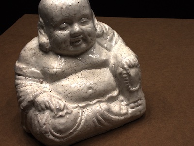
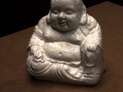
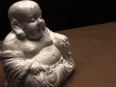
(a) Sparse Set of $3$ Input Images

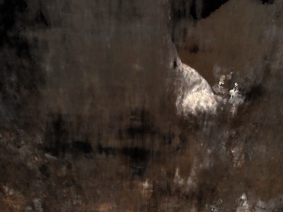
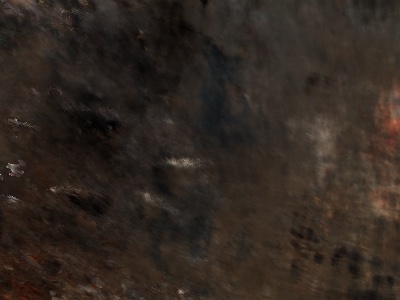
(b) Novel Views Synthesized by NeRF [36]

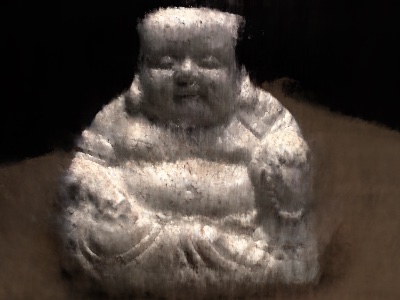
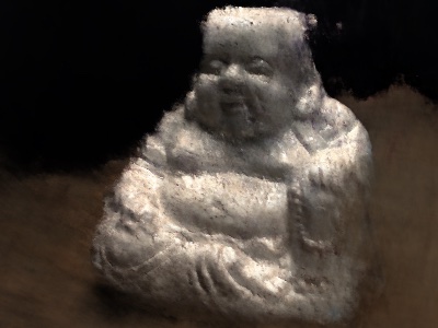
(c) Same Novel Views Synthesized by Our Method

Figure 1: View Synthesis from Sparse Inputs. While Neural Radiance Fields (NeRF) allow for state-of-the-art view synthesis if many input images are provided, results degrade when only few views are available (1(b)). In contrast, even with sparse inputs our novel regularization and optimization strategy leads to 3D-consistent representations that render realistic novel views (1(c)).

Though NeRF achieves state-of-the-art performance, it requires dense coverage of the scene. However, in real-world applications such as AR/VR, autonomous driving, and robotics, the input is typically much sparser, with only few views of any particular object or region available per scene. In this sparse setting, the quality of NeRF’s rendered novel views drops significantly (see Fig. 1).

Figure 2: Overview. NeRF optimizes the reconstruction loss for a given set of input images (blue cameras). For sparse inputs, however, this leads to degenerate solutions. In this work, we propose to sample unobserved views (red cameras) and regularize the geometry and appearance of patches rendered from those views. More specifically, we cast rays through the scene and render patches from unobserved viewpoints for a given radiance field $f_{\theta}$. We then regularize appearance by feeding the predicted RGB patches through a trained normalizing flow model $\phi$ and maximizing predicted log-likelihood. We regularize geometry by enforcing a smoothness loss on the rendered depth patches. Our approach leads to 3D-consistent representations even for sparse inputs from which realistic novel views can be rendered.

Several works have proposed conditional models to overcome these limitations [62, 8, 58, 6, 29, 56]. These models require expensive pre-training, i.e. training the model on large-scale datasets of many scenes with multi-view images and camera pose annotations, as opposed to test-time optimization which is done from scratch for a given test scene. At test time, novel views can be generated from only a few input images through amortized inference, optionally combined with per scene test time fine-tuning. Though these models achieve promising results, obtaining the necessary pre-training data by capturing or rendering many different scenes can be prohibitively expensive. Moreover, these techniques may not generalize well to novel domains at test time, and may exhibit blurry artifacts as a result of the inherent ambiguity of sparse input data.

One alternate approach is to optimize the network weights from scratch for every new scene and introduce regularization to improve the performance for sparse inputs, e.g., by adding extra supervision [23] or learning embeddings representative of the input views [19]. However, existing methods either heavily rely on external supervisory signals that might not always be available, or operate on low-resolution renderings of the scene that provide only high-level information.

Contribution:  In this paper, we present RegNeRF, a novel method for regularizing NeRF models for sparse input scenarios. Our main contributions are the following:

• A patch-based regularizer for depth maps rendered from unobserved viewpoints, which reduces floating artifacts and improves scene geometry.

• A normalizing flow model to regularize the colors predicted at unseen viewpoints by maximizing the log-likelihood of the rendered patches and thereby avoid color shifts between different views.

• An annealing strategy for sampling points along the ray, where we first sample scene content within a small range before expanding to the full scene bounds which prevents divergence early during training.

2 Related Work

Neural Representations: In 3D vision, coordinate-based neural representations [33, 44, 7, 34] have become a popular representation for various tasks such as 3D reconstruction [33, 44, 7, 45, 55, 39, 51, 1, 13, 48, 14, 57, 42], 3D-aware generative modelling [49, 38, 5, 37, 15, 41, 9, 64, 32, 16], and novel-view synthesis [36, 2, 40, 52, 61, 60, 31, 27, 22, 43, 24, 3, 12]. In contrast to traditional representations like point clouds, meshes, or voxels, this paradigm represents 3D geometry and color information in the weights of a neural network, leading to a compact representation. Several works [40, 52, 61, 36, 28] proposed differentiable rendering approaches to learn neural representations from only multi-view image supervision. Among these, Neural Radiance Fields (NeRF) [36] have emerged as a powerful method for novel-view synthesis due to its simplicity and state-of-the-art performance. In mip-NeRF [2], point-based ray tracing is replaced using cone tracing to combat aliasing. As this is a more robust representation for scenes with various camera distances and reduces NeRF’s coarse and fine MLP networks to a single multiscale MLP, we adopt mip-NeRF as our scene representation. However, compared to previous works [2, 36], we consider a much sparser input scenario in which neither NeRF nor mip-NeRF are able to produce realistic novel views. By regularizing scene geometry and appearance, we are able to synthesize high-quality renderings despite only using as few as 3 wide-baseline input images.

Sparse Input Novel-View Synthesis:  One approach for circumventing the requirement of dense inputs is to aggregate prior knowledge by pre-training a conditional model of radiance fields [62, 8, 58, 6, 29, 56, 47, 26, 20]. PixelNeRF [62] and Stereo Radiance Fields [8] use local CNN features extracted from the input images, whereas MVSNeRF [6] obtains a 3D cost volume via image warping which is then processed by a 3D CNN. Though they achieve compelling results, these methods require a multi-view image dataset of many different scenes for pre-training, which is not always readily available and may be expensive to obtain. Further, most approaches require fine-tuning the network weights at test time despite the long pre-training phase, and the quality of novel views is prone to drop when the data domain changes at test time. Tancik et al. [54] learn network initializations from which test time optimization on a new scene converges faster. This approach assumes that the training and test data are taken from the same domain, and results may degrade if the domain changes at test time.

In this work, we explore an alternative approach which avoids expensive pre-training by regularizing appearance and geometry in novel (virtual) views. Previous works in this direction include DS-NeRF [23] and DietNeRF [19]. DS-NeRF improves reconstruction accuracy by adding additional depth supervision. In contrast, our approach only uses RGB images and does not require depth input. DietNeRF [19] compares CLIP [46, 11] embeddings of unseen viewpoints rendered at low resolutions. This semantic consistency loss can only provide high-level information and does not improve scene geometry for sparse inputs. Our approach instead regularizes scene geometry and appearance based on rendered patches and applies a scene space annealing strategy. We find that our approach leads to more realistic scene geometry and more accurate novel views.

3 Method

We propose a novel optimization procedure for neural radiance fields from sparse inputs. More specifically, our approach builds upon mip-NeRF [2], which uses a multi-scale radiance field model to represent scenes (Sec. 3.1). For sparse views, we find the quality of mip-NeRF’s view synthesis drops mainly due to incorrect scene geometry and training divergence. To overcome this, we propose a patch-based approach to regularize the predicted color and geometry from unseen viewpoints (Sec. 3.2). We also provide a strategy for annealing the scene sampling bounds to avoid divergence at the beginning of training (Sec. 3.3). Finally, we use higher learning rates in combination with gradient clipping to speed up the optimization process (Sec. 3.4). Fig. 2 shows an overview of our method.

3.1 Background

Neural Radiance Fields  A radiance field is a continuous function $f$ mapping a 3D location $\mathbf{x}\in\mathbb{R}^{3}$ and viewing direction $\mathbf{d}\in\mathbb{S}^{2}$ to a volume density $\sigma\in[0,\infty)$ and color value $\mathbf{c}\in[0,1]^{3}$. Mildenhall et al. [36] parameterize this function using a multi-layer perceptron (MLP), where the weights of the MLP are optimized to reconstruct a set of input images of a particular scene:

$$\begin{split}f_{\theta}:\mathbb{R}^{L_{\mathbf{x}}}\times\mathbb{R}^{L_{\mathbf{d}}}&\to[0,1]^{3}\times[0,\infty)\\ \left(\gamma(\mathbf{x}),\gamma(\mathbf{d})\right)&\mapsto(\mathbf{c},\sigma)\,.\end{split}$$ (1)

Here, $\theta$ indicates the network weights and $\gamma$ a predefined positional encoding [36, 55] applied to $\mathbf{x}$ and $\mathbf{d}$.

Volume Rendering:  Given a neural radiance field $f_{\theta}$, a pixel is rendered by casting a ray $\mathbf{r}(t)=\mathbf{o}+t\mathbf{d}$ from the camera center $\mathbf{o}$ through the pixel along direction $\mathbf{d}$. For given near and far bounds $t_{n}$ and $t_{f}$, the pixel’s predicted color value $\hat{\mathbf{c}}_{\theta}$ is computed using alpha compositing:

$$\begin{split}\hat{\mathbf{c}}_{\theta}(\mathbf{r})=\int_{t_{n}}^{t_{f}}T(t)\sigma_{\theta}(\mathbf{r}(t))\mathbf{c}_{\theta}(\mathbf{r}(t),\mathbf{d})\,dt\\ \text{where}\quad T(t)=\exp\left(-\int_{t_{n}}^{t}\sigma_{\theta}(\mathbf{r}(s))\,ds\right)\,,\end{split}$$ (2)

and $\sigma_{\theta}(\cdot)$ and $\mathbf{c}_{\theta}(\cdot,\cdot)$ indicate the density and color prediction of radiance field $f_{\theta}$, respectively. In practice, these integrals are approximated using quadrature [36]. A neural radiance field is optimized over a set of input images and their camera poses by minimizing the mean squared error

$$\mathcal{L}_{\text{MSE}}(\theta,\mathcal{R}_{i})=\sum_{\mathbf{r}\in\mathcal{R}_{i}}\left\|\hat{\mathbf{c}}_{\theta}(\mathbf{r})-\mathbf{c}_{\text{GT}}(\mathbf{r})\right\|^{2}\,,$$ (3)

where $\mathcal{R}_{i}$ indicates a set of input rays and $\mathbf{c}_{\text{GT}}$ its GT color.

mip-NeRF:  While NeRF only casts a single ray per pixel, mip-NeRF [2] instead casts a cone. The positional encoding changes from representing an infinitesimal point to an integration over a volume covered by a conical frustum. This is a more appropriate representation for scenes with varying camera distances and allows NeRF’s coarse and fine MLPs to be combined into a single multiscale MLP, thereby increasing training speed and reducing model size. We adopt the mip-NeRF representation in this work.

3.2 Patch-based Regularization

NeRF’s performance drops significantly if the number of input views is sparse. Why is this the case? Analyzing its optimization procedure, the model is only supervised from these sparse viewpoints by the reconstruction loss in (3). While it learns to reconstruct the input views perfectly, novel views may be degenerate because the model is not biased towards learning a 3D consistent solution in such a sparse input scenario (see Fig. 1). To overcome this limitation, we regularize unseen viewpoints. More specifically, we define a space of unseen but relevant viewpoints and render small patches randomly sampled from these cameras. Our key idea is that these patches can be regularized to yield smooth geometry and high-likelihood colors.

Unobserved Viewpoint Selection:  To apply regularization techniques for unobserved viewpoints, we must first define the sample space of unobserved camera poses. We assume a known set of target poses $\left\{\mathbf{P}^{i}_{\text{target}}\right\}_{i}$ where

$$\mathbf{P}_{\text{target}}^{i}=\left[\mathbf{R}^{i}_{\text{target}}|\mathbf{t}^{i}_{\text{target}}\right]\in SE(3)\,.$$ (4)

These target poses can be thought of bounding the set of poses from which we would like to render novel views at test time. We define the space of possible camera locations as the bounding box of all given target camera locations

$$\mathcal{S}_{t}=\left\{\mathbf{t}\in\mathbb{R}^{3}\mid\mathbf{t}_{\text{min}}\leq\mathbf{t}\leq\mathbf{t}_{\text{max}}\right\}$$ (5)

where $\mathbf{t}_{\text{min}}$ and $\mathbf{t}_{\text{max}}$ are the elementwise minimum and maximum values of $\left\{\mathbf{t}^{i}_{\text{target}}\right\}_{i}$, respectively.

To obtain the sample space of camera rotations, we assume that all cameras roughly focus on a central scene point. We define a common “up” axis $\bar{\mathbf{p}}_{u}$ by computing the normalized mean over the up axes of all target poses. Next, we calculate a mean focus point $\bar{\mathbf{p}}_{f}$ by solving a least squares problem to determine the 3D point with minimum squared distance to the optical axes of all target poses. To learn more robust representations, we add random jitter to the focal point before calculating the camera rotation matrix. We define the set of of all possible camera rotations (given the sampled position $\mathbf{t}$) as

$$\mathcal{S}_{R}|\mathbf{t}=\left\{\mathbf{R}(\bar{\mathbf{p}}_{u},\bar{\mathbf{p}}_{f}+\mathbf{\epsilon},\mathbf{t})\mid\mathbf{\mathbf{\epsilon}}\sim\mathcal{N}(0,0.125)\right\}$$ (6)

where $\mathbf{R}(\cdot,\cdot,\cdot)$ indicates the resulting “look-at” camera rotation matrix and $\epsilon$ is a small jitter added to the focus point. We obtain a random camera pose by sampling a position and rotation:

$$\mathcal{S}_{P}=\left\{\left[\mathbf{R}|\mathbf{t}\right]|\mathbf{R}\sim\mathcal{S}_{R}|\mathbf{t},\mathbf{t}\sim\mathcal{S}_{t}\right\}$$ (7)

Geometry Regularization:  It is well-known that real-world geometry tends to be piece-wise smooth, i.e., flat surfaces are more likely than high-frequency structures [18]. We incorporate this prior into our model by encouraging depth smoothness from unobserved viewpoints. Similarly to how a pixel’s color is rendered in (2), we calculate the expected depth as:

$$\begin{split}\hat{d_{\theta}}(\mathbf{r})=\int_{t_{n}}^{t_{f}}T(t)\sigma_{\theta}(\mathbf{r}(t))t\,dt\,.\end{split}$$ (8)

We formulate our depth smoothness loss as

$$\begin{split}\mathcal{L}_{\text{DS}}(\theta,\mathcal{R}_{r})=\sum_{\mathbf{r}\in\mathcal{R}_{r}}\sum_{i,j=1}^{S_{\text{patch}}-1}&\left(\hat{d_{\theta}}(\mathbf{r}_{ij})-\hat{d_{\theta}}(\mathbf{r}_{i+1j})\right)^{2}\\ +&\left(\hat{d_{\theta}}(\mathbf{r}_{ij})-\hat{d_{\theta}}(\mathbf{r}_{ij+1})\right)^{2}\,,\end{split}$$ (9)

where $\mathcal{R}_{r}$ indicates a set of rays sampled from camera poses $\mathcal{S}_{P}$, $\mathbf{r}_{ij}$ is the ray through pixel $(i,j)$ of a patch centered at $\mathbf{r}$, and $S_{\text{patch}}$ is the size of the rendered patches.

Color Regularization:  We observe that for sparse inputs, the majority of artifacts are caused by incorrect scene geometry. However, even with correct geometry, optimizing a NeRF model can still lead to color shifts or other errors in scene appearance prediction due to the sparsity of the inputs. To avoid degenerate colors and ensure stable optimization, we also regularize color prediction. Our key idea is to estimate the likelihood of rendered patches and maximize it during optimization. To this end, we make use of readily-available unstructured 2D image datasets. Note that, while datasets of posed multi-view images are expensive to collect, collections of unstructured natural images are abundant. Our only criterion for the dataset is that it contains diverse natural images, allowing us to reuse the same flow model for any type of real-world scene we reconstruct. We train a RealNVP [10] normalizing flow model on patches from the JFT-300M dataset [53]. With this trained flow model we estimate the log-likelihoods (LL) of rendered patches and maximize them during optimization. Let

$$\phi:[0,1]^{S_{\text{patch}}\times S_{\text{patch}}\times 3}\to\mathbb{R}^{d}$$ (10)

be the learned bijection mapping an RGB patch of size $S_{\text{patch}}=8$ to $\mathbb{R}^{d}$ where $d=S_{\text{patch}}\cdot S_{\text{patch}}\cdot 3$. We define our color regularization loss as

$$\begin{split}\mathcal{L}_{\text{NLL}}(\theta,\mathcal{R}_{r})=\sum_{\mathbf{r}\in\mathcal{R}_{r}}-\log p_{Z}\left(\phi\left(\hat{P}_{r}\right)\right)\\ \text{where }\hat{P}_{r}=\left\{\hat{\mathbf{c}}_{\theta}(\mathbf{r}_{ij})\mid 1\leq i,j\leq S_{\text{patch}}\right\}\end{split}$$ (11)

and $\mathcal{R}_{r}$ indicates a set of rays sampled from $\mathcal{S}_{P}$, $\hat{P}_{r}$ the predicted RGB color patch with center $\mathbf{r}$, and $-\log p_{Z}$ the negative log-likelihood (“NLL”) with Gaussian $p_{Z}$.

Total Loss:  The total loss we optimize in each iteration is

$$\mathcal{L}(\theta)=\mathcal{L}_{\text{MSE}}(\theta,\mathcal{R}_{i})+\mathcal{L}_{\text{DS}}(\theta,\mathcal{R}_{r})+\mathcal{L}_{\text{NLL}}(\theta,\mathcal{R}_{r})$$ (12)

where $\mathcal{R}_{i}$ indicates a set of rays from input poses, and $\mathcal{R}_{r}$ a set of rays from random poses $\mathcal{S}_{P}$.

3.3 Sample Space Annealing

For very sparse scenarios (e.g., 3 or 6 input views), we observe another failure mode of NeRF: divergent behavior at the start of training. This leads to high density values at ray origins. While input views are correctly reconstructed, novel views degenerate as no 3D-consistent representation is recovered. We find that annealing the sampled scene space quickly over the early iterations during optimization helps to avoid this problem. By restricting the scene sampling space to a smaller region defined for all input images, we introduce an inductive bias to explain the input images with geometric structure in the center of the scene.

Recall from (2) that $t_{n},t_{f}$ are the camera’s near and far plane, respectively, and let $t_{m}$ be a defined center point (usually the midpoint between $t_{n}$ and $t_{f}$). We define

$$\begin{split}t_{n}(i)&=t_{m}+(t_{n}-t_{m})\eta(i)\\ t_{f}(i)&=t_{m}+(t_{f}-t_{m})\eta(i)\\ \eta(i)&=\mathrm{max}\left(\mathrm{min}\left(\nicefrac{{i}}{{N_{t}}},\,p_{s}\right),\,1\right)\end{split}$$ (13)

where $i$ indicates the current training iteration, $N_{t}$ a hyperparameter indicating how many iterations until the full range is reached, and $p_{s}$ a hyperparameter indicating a start range (e.g., $0.5$). This annealing is applied to renderings from both the input poses and the sampled unobserved viewpoints. We find that this annealing strategy ensures stability during early training and avoids degenerate solutions.

3.4 Training Details

We build our code on top of of the JAX [4] mip-NeRF codebase. We optimize with Adam [25] using an exponential learning rate decay from $2\cdot 10^{-3}$ to $2\cdot 10^{-5}$. We clip gradients by value at $0.1$ and then by norm at $0.1$. We train for $500$ pixel epochs, e.g., $44$K, $88$K, and $132$K iterations on DTU for $3/6/9$ input views respectively (all fewer iterations than mip-NeRF’s default $250$K steps [36]).

4 Experiments

(a) Sparse Set of 3 Input Views

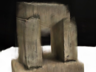
(b) PixelNeRF
(PSNR: $17.37/16.89$)

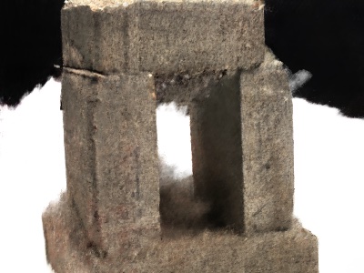
(c) Our Method
(PSNR: $8.79/20.08$)

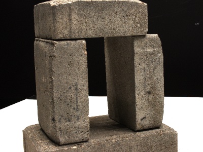
(d) GT

Figure 3: Evaluation Bias. Many scenes in DTU are composed of an object on a white table with black background resulting in an evaluation bias favoring a correct background over the object-of-interest. For sparse inputs the background may only be partially observed in the input views and strongly overfitting to the table is incentivized, though most real-world applications would prefer to accurately reconstruct the object-of-interest. Here we show an example with full image (first) and object-of-interest (second) PSNR for PixelNeRF (which drops from $17.37$ to $16.89$) and for our method (which improves from $8.79$ to $20.08$).

Datasets  We report results on the real world multi-view datasets DTU [21] and LLFF [35]. DTU contains images of objects placed on a table, and LLFF consists of complex forward-facing scenes. For DTU, we observe that in scenes with a white table and a black background, the model is heavily penalized for incorrect background predictions regardless of the quality of the rendered object-of-interest (see Fig. 3). To avoid this background bias, we evaluate all methods with the object masks applied to the rendered images (full image evaluations in supp. mat.). We adhere to the protocol of Yu et al. [62] and evaluate on their reported test set of $15$ scenes. For LLFF, we adhere to community standards [36] and use every $8$-th image as the held-out test set and select the input views evenly from the remaining images. Following previous work [62], we report results for the scenarios of $3$, $6$, and $9$ input views.

Metrics:  We report the mean of PSNR, structural similarity index (SSIM) [59], and the LPIPS perceptual metric  [63]. To ease comparison, we also report the geometric mean of $\text{MSE}=10^{-\text{PSNR}/10}$, $\sqrt{1-\text{SSIM}}$, and LPIPS [2].

mip-NeRF [2]

Ours

mip-NeRF [2]

Ours

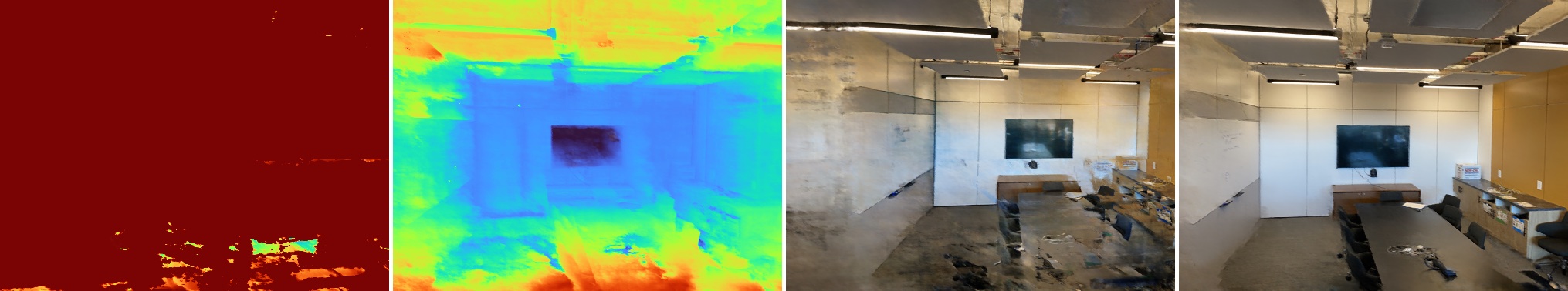
(a) 3 Input Views

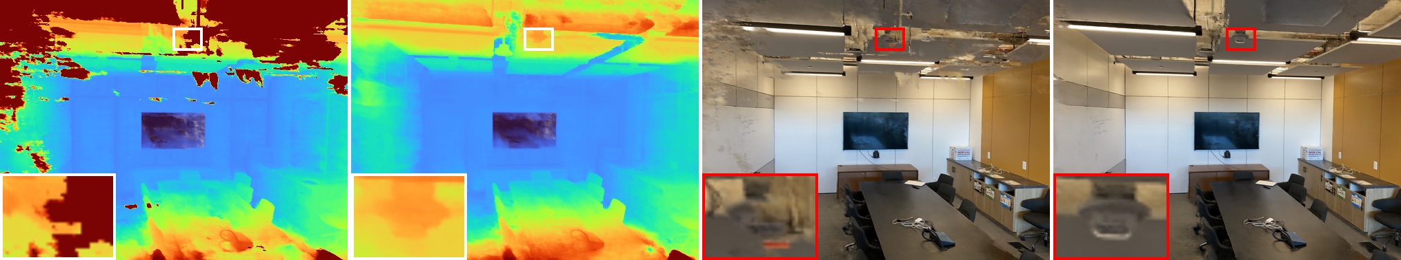
(b) 6 Input Views

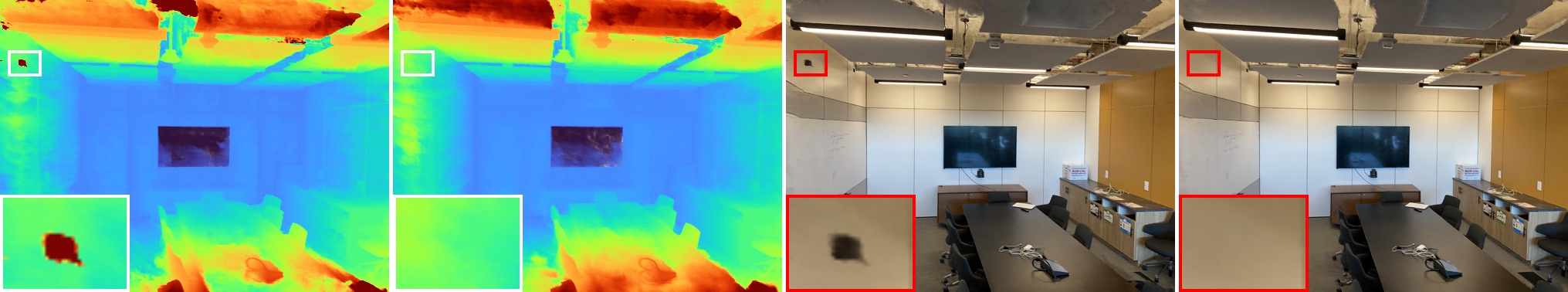
(c) 9 Input Views

Figure 4: Importance of Geometry. We compare expected depth maps (left) and RGB renderings (right) for mip-NeRF [2] and our method on the LLFF dataset. The quality of optimized geometry is correlated with view synthesis performance: Our proposed scene space annealing and geometry regularization strategies remove floating artifacts (see zoom-in) and lead to smooth geometry, which in turn leads to improved quality of rendered novel views.

Baselines:  We compare against the state-of-the-art conditional models PixelNeRF [62], Stereo Radiance Fields (SRF) [8], and MVSNeRF [6]. We re-train PixelNeRF for the $6/9$ view scenarios, leading to better results, and we similarly pre-train SRF with $3/6/9$ views. We pre-train all methods on the large-scale DTU dataset. The LLFF dataset has been shown to be too small for pre-training [23] and hence serves as an out-of-distribution test for conditional models. We report the conditional models on both datasets also after additional per-scene test time optimization (“ft” for “fine-tuned”). Further, we compare against mip-NeRF [2] and DietNeRF [19] which do not require pre-training, as with our approach. As no official code is available, we reimplement DietNeRF on top of the mip-NeRF codebase (achieving better results) and train both methods for $250$K iterations per scene with exponential learning rate decay from $5\cdot 10^{-4}$ to $5\cdot 10^{-5}$.

4.1 View Synthesis from Sparse Inputs

We first compare our model to the vanilla mip-NeRF baseline, analyzing the effect of our regularizers on scene geometry, appearance and data efficiency.

	Setting	PSNR $\uparrow$			SSIM $\uparrow$			LPIPS $\downarrow$			Average $\downarrow$
		3-view	6-view	9-view	3-view	6-view	9-view	3-view	6-view	9-view	3-view	6-view	9-view
SRF [8]	Trained on DTU	15.32	17.54	18.35	0.671	0.730	0.752	0.304	0.250	0.232	0.171	0.132	0.120
PixelNeRF [62]		16.82	19.11	20.40	0.695	0.745	0.768	0.270	0.232	0.220	0.147	0.115	0.100
MVSNeRF [6]		yellow!2518.63	orange!2520.70	22.40	red!250.769	orange!250.823	yellow!250.853	orange!250.197	yellow!250.156	yellow!250.135	orange!250.113	orange!250.088	0.068
SRF ft [8]	Trained on DTU and Optimized per Scene	15.68	18.87	20.75	0.698	0.757	0.785	0.281	0.225	0.205	0.162	0.114	0.093
PixelNeRF ft [62]		red!2518.95	20.56	21.83	0.710	0.753	0.781	0.269	0.223	0.203	0.125	0.104	0.090
MVSNeRF ft [6]		18.54	20.49	22.22	red!250.769	yellow!250.822	yellow!250.853	orange!250.197	orange!250.155	yellow!250.135	orange!250.113	yellow!250.089	0.069
mip-NeRF [2]	Optimized per Scene	8.68	16.54	yellow!2523.58	0.571	0.741	orange!250.879	0.353	0.198	orange!250.092	0.323	0.148	orange!250.056
DietNeRF [19]		11.85	yellow!2520.63	orange!2523.83	0.633	0.778	0.823	0.314	0.201	0.173	0.243	0.101	yellow!250.068
Ours		orange!2518.89	red!2522.20	red!2524.93	yellow!250.745	red!250.841	red!250.884	red!250.190	red!250.117	red!250.089	red!250.112	red!250.071	red!250.047

Table 1: Quantitative Comparison on DTU. For $3$ input views, our model achieves quantitative results comparable to conditional models (SRF, PixelNeRF, MVSNeRF) despite not requiring an expensive pre-training phase, and strongly outperforms other baselines (mip-NeRF, DietNeRF) which operate in the same setting as us. For $6$ and $9$ input views, our model achieves the best overall quantitative results.

	Setting	PSNR $\uparrow$			SSIM $\uparrow$			LPIPS $\downarrow$			Average $\downarrow$
		3-view	6-view	9-view	3-view	6-view	9-view	3-view	6-view	9-view	3-view	6-view	9-view
SRF [8]	Trained on DTU	12.34	13.10	13.00	0.250	0.293	0.297	0.591	0.594	0.605	0.313	0.293	0.296
PixelNeRF [62]		7.93	8.74	8.61	0.272	0.280	0.274	0.682	0.676	0.665	0.461	0.433	0.432
MVSNeRF [6]		yellow!2517.25	19.79	20.47	yellow!250.557	0.656	0.689	yellow!250.356	0.269	0.242	yellow!250.171	0.125	0.111
SRF ft [8]	Trained on DTU and Optimized per Scene	17.07	16.75	17.39	0.436	0.438	0.465	0.529	0.521	0.503	0.203	0.207	0.193
PixelNeRF ft [62]		16.17	17.03	18.92	0.438	0.473	0.535	0.512	0.477	0.430	0.217	0.196	0.163
MVSNeRF ft [6]		orange!2517.88	19.99	20.47	orange!250.584	0.660	0.695	red!250.327	0.264	0.244	orange!250.157	0.122	0.111
mip-NeRF [2]	Optimized per Scene	14.62	yellow!2520.87	yellow!2524.26	0.351	yellow!250.692	orange!250.805	0.495	yellow!250.255	orange!250.172	0.246	yellow!250.114	orange!250.073
DietNeRF [19]		14.94	orange!2521.75	orange!2524.28	0.370	orange!250.717	yellow!250.801	0.496	orange!250.248	yellow!250.183	0.240	orange!250.105	orange!250.073
Ours		red!2519.08	red!2523.10	red!2524.86	red!250.587	red!250.760	red!250.820	orange!250.336	red!250.206	red!250.161	red!250.146	red!250.086	red!250.067

Table 2: Quantitative Comparison on LLFF. Some conditional models (SRF, PixelNeRF) overfit to the training data (DTU) but all benefit from additional fine-tuning at test time. The two unconditional baselines mip-NeRF and DietNeRF do not achieve competitive results for $3$ input views, but outperform conditional models for the $6/9$ input view scenarios. Our method achieves the best results for all scenarios.

Geometry Prediction:  We observe that novel view synthesis performance is directly correlated with how accurately the scene geometry is predicted: in Fig. 4 we show expected depth maps and RGB renderings for mip-NeRF and our method on the LLFF room scene. We find that for $3$ input views, mip-NeRF produces low-quality renderings and poor geometry. In contrast, our method produces an acceptable novel view and a realistic scene geometry, despite the low number of inputs. When increasing the number of input images to $6$ or $9$, mip-NeRF’s predicted geometry improves but still contains floating artifacts. Our method generates smooth scene geometry, which is reflected in its higher-quality novel views.

Data Efficiency:

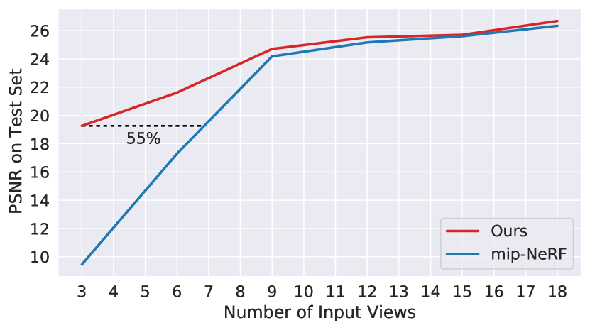
Figure 5: Data Efficiency. In sparse settings, our method requires up to $55\%$ fewer images than mip-NeRF [2] to achieve a similar test set performance on the DTU dataset.

To evaluate our gain in data efficiency, we train mip-NeRF and our method for various numbers of input views and compare their performance. We find that for sparse inputs our method requires up to $55\%$ fewer input views to match mip-NeRF’s mean PSNR on the test set, where the difference is larger for fewer input views. For $18$ input views, both methods achieve a similar performance (as this work focuses on sparse inputs, tuning hyper-parameters for more input views could result in improved performance for these scenarios).

4.2 Baseline Comparison

PixelNeRF [62]

MVSNeRF [6]

DietNeRF [19]

Ours

GT

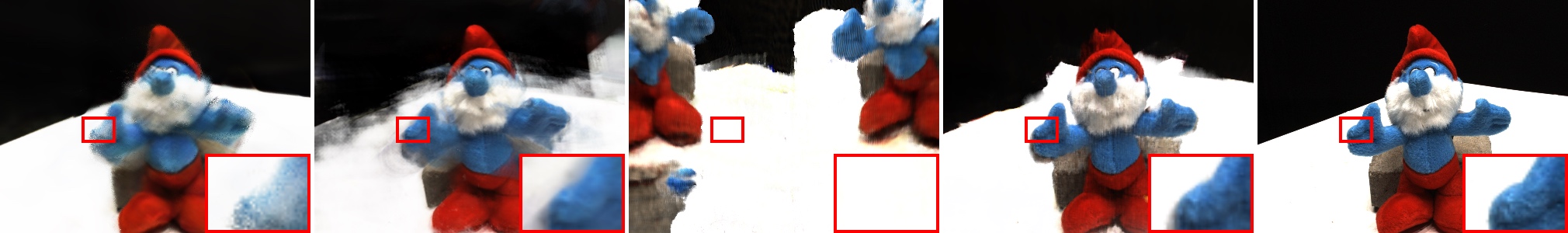
(a) 3 Input Views

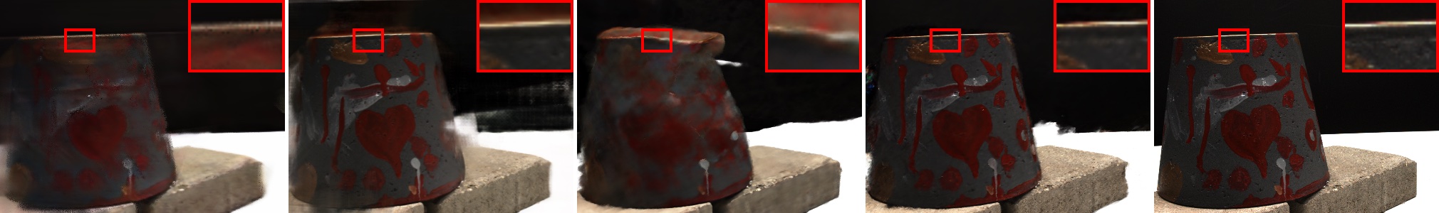
(b) 6 Input Views

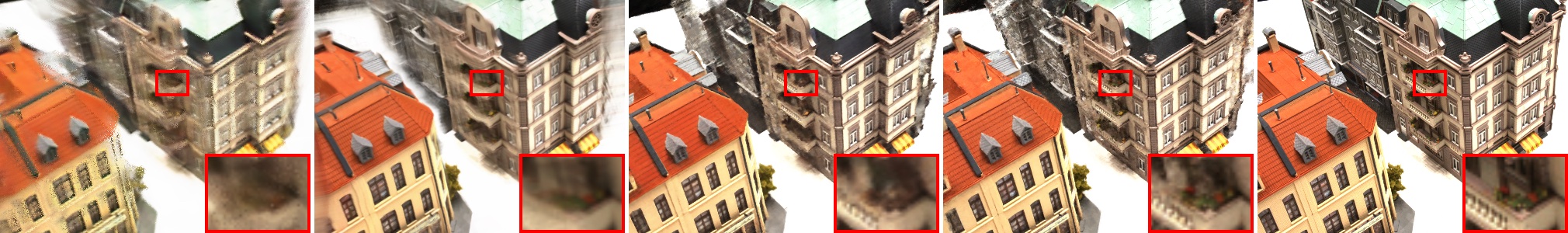
(c) 9 Input Views

Figure 6: View Synthesis on DTU. We show novel views generated by the baselines and our method for $3$, $6$ and $9$ input images. While the baselines suffer from blurriness or incorrect scene geometry, our approach leads to sharp novel views. For $3$ input views, DietNeRF leads to wrong geometry prediction and blends the input images rather than obtaining a 3D-consistent representation, due to the global nature of its semantic consistency loss.

PixelNeRF [62]

PixelNeRF ft [62]

MVSNeRF ft [6]

DietNeRF [19]

Ours

GT

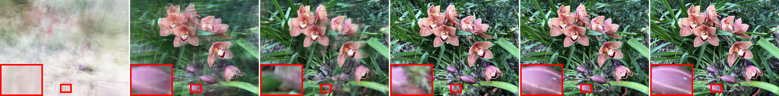
(a) 3 Input Views

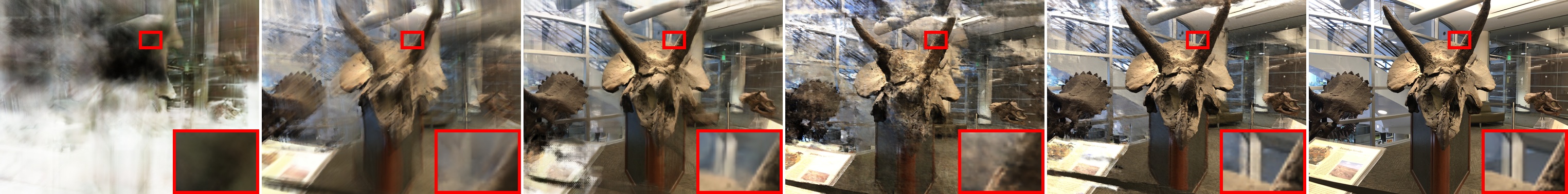
(b) 6 Input Views

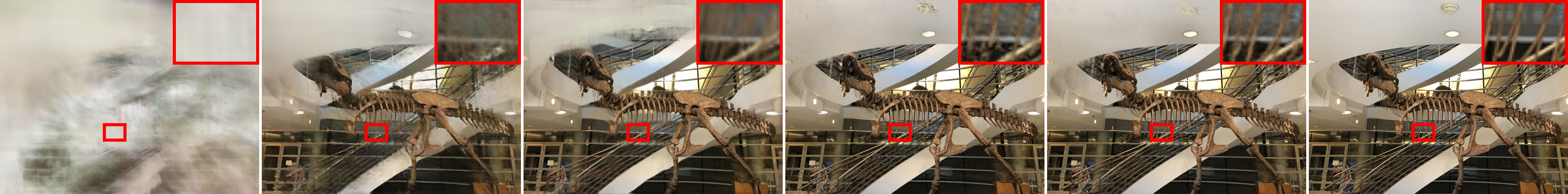
(c) 9 Input Views

Figure 7: View Synthesis on LLFF. Conditional models overfit to the training data and hence perform poorly on test data from a novel domain. Further, novel views still appear slightly blurry despite additional fine-tuning (“ft”). While DietNeRF does not require expensive pre-training similiar to our approach, our method leads to more accurate scene geometry, resulting in sharper and more realistic renderings.

DTU Dataset  For $3$ input views, our method achieves quantitative results comparable to the best-performing conditional models (see Tab. 1) which are pre-trained on other DTU scenes. Compared to the other methods that also do not require pre-training, we achieve the best results. For $6$ and $9$ input views, our approach performs best compared to all baselines. As evidenced by Fig. 6, we see that conditional models are able to predict good overall novel views, but become blurry particularly around edges and exhibit less consistent appearance for novel views whose cameras are far from the input views. For mip-NeRF and DietNeRF, which are not pre-trained (like our method), geometry prediction and hence synthesized novel views degrade for very sparse scenarios. Even with $6$ or $9$ input views, the results contain floating artifacts and incorrect geometry. In contrast, our approach performs well across all scenarios, producing sharp results with more accurate scene geometry.

LLFF Dataset:  For conditional models, the LLFF dataset serves as an out-of-distribution scenario as the models are trained on DTU. We observe that SRF and PixelNeRF appear to overfit to the training data, which leads to low quantitative results (see Tab. 2). MVSNeRF generalizes better to novel data, and all three models benefit from additional fine-tuning. For $3$ input views, mip-NeRF and DietNeRF are not able to generate competitive novel views. However, with $6$ or $9$ input views, they outperform the best conditional models. Despite requiring fewer optimization steps than mip-NeRF and DietNeRF and no pre-training at all, our method achieves the best results across all scenarios. From Fig. 7 we observe that the predictions from conditional models tend to be blurry for views far away from the inputs, and the test-time optimized baselines contain errors in predicted scene geometry. Our method achieves superior geometry predictions and more realistic novel views.

4.3 Ablation Studies

	PSNR $\uparrow$	SSIM $\uparrow$	LPIPS $\downarrow$	Average $\downarrow$
w/o Scene Space Ann.	10.17	0.613	0.332	0.291
w/o Geometry Reg.	yellow!2514.34	yellow!250.689	yellow!250.246	yellow!250.188
w/o Appearance Reg.	orange!2518.34	orange!250.742	orange!250.191	orange!250.117
Ours	red!2518.89	red!250.745	red!250.190	red!250.112

Table 3: Ablation Study. We report our method ablating components on the DTU dataset for $3$ input views. For very sparse scenarios, we find that scene space annealing is crucial to avoid degenerate solutions. Further, regularizing scene geometry has a bigger impact on the performance than appearance regularization. Combining all components leads to the best performance.

In Tab. 3, we ablate various components of our method. For sparse inputs, we find that the proposed scene space annealing strategy avoids degenerate solutions. Further, regularizing geometry is more important than appearance, and combining all components leads to the best results.

Ablation of Geometry Regularizer:

	PSNR $\uparrow$	SSIM $\uparrow$	LPIPS $\downarrow$	Average $\downarrow$
Opacity Reg. [30]	11.07	0.617	0.309	0.268
Ray Density Entropy Reg.	13.93	0.680	0.254	0.198
Normal Smooth. Reg. [40]	14.22	0.683	0.251	0.193
Density Surface Reg.	yellow!2514.71	yellow!250.687	yellow!250.247	yellow!250.184
Sparsity Reg. [17]	orange!2516.77	orange!250.711	orange!250.221	orange!250.145
Depth Smooth. Reg. (Ours)	red!2518.89	red!250.745	red!250.190	red!250.112

Table 4: Geometry Regularization. We compare different choices of geometry regularization strategies on DTU ($3$ input views) and find that our depth smoothness prior performs best.

In Tab. 4, we investigate the performance of other geometry regularization techniques. We find that opacity-based regularizers (e.g., enforce rendered opacity values near to either $0$ or $1$) and density or normal smoothness priors (e.g. minimize the distance between neighboring normal vectors in 3D), two strategies often used to enforce solid and smooth surfaces, do not produce accurate scene geometry. Employing the sparsity prior from Hedman et al. [17] leads to better quantitative results, but novel views still contain floating artifacts and the optimized geometry has holes. In contrast, our geometry regularization strategy achieves the best performance. We hypothesize that similar to density-based [36] vs. single surface optimization [40, 52] for coordinate-based methods, providing gradient information along the full ray rather than a single point provides a more stable and informative learning signal.

5 Conclusion

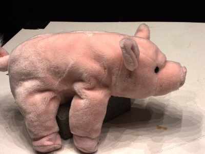
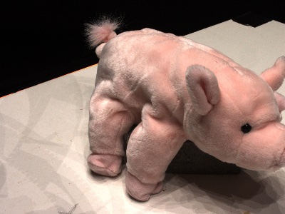
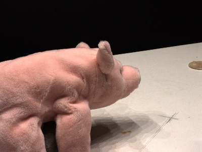
(a) Sparse Set of 3 Input Views

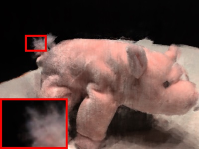
(b) Prediction

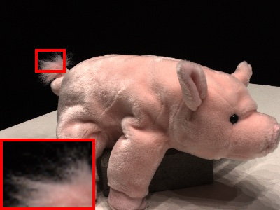
(c) GT

Figure 8: Failure Analysis. As we do not attempt to hallucinate geometric details in this work, our model may lead to blurry predictions in unobserved regions with areas of fine geometry (8(b)). We identify incorporating uncertainty prediction or generative components into our model as interesting future work.

We have presented RegNeRF, a novel approach for optimizing Neural Radiance Fields (NeRF) in data-limited regimes. Our key insight is that for sparse input scenarios, NeRF’s performance drops significantly due to incorrectly optimized scene geometry and divergent behavior at the start of optimization. To overcome this limitation, we propose techniques to regularize the geometry and appearance of rendered patches from unseen viewpoints. In combination with a novel sample-space annealing strategy, our method is able to learn 3D-consistent representations from which high-quality novel views can be synthesized. Our experimental evaluation shows that our model outperforms not only methods that, similar to us, only optimize over a single scene, but in many cases also conditional models that are extensively pre-trained on large scale multi-view datasets.

Limitations and Future Work:  In this work, we do not attempt to hallucinate geometric detail. As a result, our model may lead to blurry predictions in unobserved areas with fine geometric structures (see Fig. 8). We identify incorporating uncertainty prediction mechanisms [50] or generative components [49, 38, 5, 15] as promising future work.

References

- [1] Matan Atzmon, Niv Haim, Lior Yariv, Ofer Israelov, Haggai Maron, and Yaron Lipman. Controlling neural level sets. In Advances in Neural Information Processing Systems (NIPS), 2019.
- [2] Jonathan T. Barron, Ben Mildenhall, Matthew Tancik, Peter Hedman, Ricardo Martin-Brualla, and Pratul P. Srinivasan. Mip-nerf: A multiscale representation for anti-aliasing neural radiance fields. In Proc. of the IEEE International Conf. on Computer Vision (ICCV), 2021.
- [3] Alexander W. Bergman, Petr Kellnhofer, and Gordon Wetzstein. Fast training of neural lumigraph representations using meta learning. In Advances in Neural Information Processing Systems (NeurIPS), 2021.
- [4] James Bradbury, Roy Frostig, Peter Hawkins, Matthew James Johnson, Chris Leary, Dougal Maclaurin, George Necula, Adam Paszke, Jake VanderPlas, Skye Wanderman-Milne, and Qiao Zhang. JAX: composable transformations of Python+NumPy programs, 2018.
- [5] Eric Chan, Marco Monteiro, Petr Kellnhofer, Jiajun Wu, and Gordon Wetzstein. pi-gan: Periodic implicit generative adversarial networks for 3d-aware image synthesis. In Proc. IEEE Conf. on Computer Vision and Pattern Recognition (CVPR), 2021.
- [6] Anpei Chen, Zexiang Xu, Fuqiang Zhao, Xiaoshuai Zhang, Fanbo Xiang, Jingyi Yu, and Hao Su. Mvsnerf: Fast generalizable radiance field reconstruction from multi-view stereo. In Proc. of the IEEE International Conf. on Computer Vision (ICCV), 2021.
- [7] Zhiqin Chen and Hao Zhang. Learning implicit fields for generative shape modeling. In Proc. IEEE Conf. on Computer Vision and Pattern Recognition (CVPR), 2019.
- [8] Julian Chibane, Aayush Bansal, Verica Lazova, and Gerard Pons-Moll. Stereo radiance fields (SRF): learning view synthesis for sparse views of novel scenes. In Proc. IEEE Conf. on Computer Vision and Pattern Recognition (CVPR), 2021.
- [9] Terrance DeVries, Miguel Angel Bautista, Nitish Srivastava, Graham W. Taylor, and Joshua M. Susskind. Unconstrained scene generation with locally conditioned radiance fields. In Proc. of the IEEE International Conf. on Computer Vision (ICCV), 2021.
- [10] Laurent Dinh, Jascha Sohl-Dickstein, and Samy Bengio. Density estimation using real NVP. In Proc. of the International Conf. on Learning Representations (ICLR), 2017.
- [11] Alexey Dosovitskiy, Lucas Beyer, Alexander Kolesnikov, Dirk Weissenborn, Xiaohua Zhai, Thomas Unterthiner, Mostafa Dehghani, Matthias Minderer, Georg Heigold, Sylvain Gelly, Jakob Uszkoreit, and Neil Houlsby. An image is worth 16x16 words: Transformers for image recognition at scale. In Proc. of the International Conf. on Learning Representations (ICLR), 2021.
- [12] Chen Gao, Yichang Shih, Wei-Sheng Lai, Chia-Kai Liang, and Jia-Bin Huang. Portrait neural radiance fields from a single image. arXiv.org, 2020.
- [13] Kyle Genova, Forrester Cole, Daniel Vlasic, Aaron Sarna, William T Freeman, and Thomas Funkhouser. Learning shape templates with structured implicit functions. In Proc. of the IEEE International Conf. on Computer Vision (ICCV), 2019.
- [14] Amos Gropp, Lior Yariv, Niv Haim, Matan Atzmon, and Yaron Lipman. Implicit geometric regularization for learning shapes. In Proc. of the International Conf. on Machine learning (ICML), 2020.
- [15] Jiatao Gu, Lingjie Liu, Peng Wang, and Christian Theobalt. Stylenerf: A style-based 3d-aware generator for high-resolution image synthesis. arXiv.org, 2021.
- [16] Zekun Hao, Arun Mallya, Serge Belongie, and Ming-Yu Liu. GANcraft: Unsupervised 3D Neural Rendering of Minecraft Worlds. In Proc. of the IEEE International Conf. on Computer Vision (ICCV), 2021.
- [17] Peter Hedman, Pratul P. Srinivasan, Ben Mildenhall, Jonathan T. Barron, and Paul Debevec. Baking neural radiance fields for real-time view synthesis. In Proc. of the IEEE International Conf. on Computer Vision (ICCV), 2021.
- [18] Jinggang Huang, Ann B. Lee, and David Mumford. Statistics of range images. In Proc. IEEE Conf. on Computer Vision and Pattern Recognition (CVPR), 2000.
- [19] Ajay Jain, Matthew Tancik, and Pieter Abbeel. Putting nerf on a diet: Semantically consistent few-shot view synthesis. In Proc. of the IEEE International Conf. on Computer Vision (ICCV), 2021.
- [20] Wonbong Jang and Lourdes Agapito. Codenerf: Disentangled neural radiance fields for object categories. In Proc. of the IEEE International Conf. on Computer Vision (ICCV), 2021.
- [21] Rasmus Ramsbøl Jensen, Anders Lindbjerg Dahl, George Vogiatzis, Engil Tola, and Henrik Aanæs. Large scale multi-view stereopsis evaluation. In Proc. IEEE Conf. on Computer Vision and Pattern Recognition (CVPR), 2014.
- [22] Yue Jiang, Dantong Ji, Zhizhong Han, and Matthias Zwicker. Sdfdiff: Differentiable rendering of signed distance fields for 3d shape optimization. In Proc. IEEE Conf. on Computer Vision and Pattern Recognition (CVPR), 2020.
- [23] Jun-Yan Zhu Kangle Deng, Andrew Liu and Deva Ramanan. Depth-supervised nerf: Fewer views and faster training for free. arXiv.org, 2021.
- [24] Petr Kellnhofer, Lars C Jebe, Andrew Jones, Ryan Spicer, Kari Pulli, and Gordon Wetzstein. Neural lumigraph rendering. In Proc. IEEE Conf. on Computer Vision and Pattern Recognition (CVPR), 2021.
- [25] Diederik P. Kingma and Jimmy Ba. Adam: A method for stochastic optimization. In Proc. of the International Conf. on Learning Representations (ICLR), 2015.
- [26] Jiaxin Li, Zijian Feng, Qi She, Henghui Ding, Changhu Wang, and Gim Hee Lee. Mine: Towards continuous depth mpi with nerf for novel view synthesis. In Proc. of the IEEE International Conf. on Computer Vision (ICCV), 2021.
- [27] Lingjie Liu, Jiatao Gu, Kyaw Zaw Lin, Tat-Seng Chua, and Christian Theobalt. Neural sparse voxel fields. In Advances in Neural Information Processing Systems (NeurIPS), 2020.
- [28] Shichen Liu, Shunsuke Saito, Weikai Chen, and Hao Li. Learning to infer implicit surfaces without 3d supervision. In Advances in Neural Information Processing Systems (NIPS), 2019.
- [29] Yuan Liu, Sida Peng, Lingjie Liu, Qianqian Wang, Peng Wang, Theobalt Christian, Xiaowei Zhou, and Wenping Wang. Neural rays for occlusion-aware image-based rendering. arXiv.org, 2021.
- [30] Stephen Lombardi, Tomas Simon, Jason Saragih, Gabriel Schwartz, Andreas Lehrmann, and Yaser Sheikh. Neural volumes: Learning dynamic renderable volumes from images. In ACM Trans. on Graphics, 2019.
- [31] Ricardo Martin-Brualla, Noha Radwan, Mehdi S. M. Sajjadi, Jonathan T. Barron, Alexey Dosovitskiy, and Daniel Duckworth. NeRF in the Wild: Neural Radiance Fields for Unconstrained Photo Collections. In Proc. IEEE Conf. on Computer Vision and Pattern Recognition (CVPR), 2021.
- [32] Quan Meng, Anpei Chen, Haimin Luo, Minye Wu, Hao Su, Lan Xu, Xuming He, and Jingyi Yu. Gnerf: Gan-based neural radiance field without posed camera. In Proc. of the IEEE International Conf. on Computer Vision (ICCV), volume abs/2103.15606, 2021.
- [33] Lars Mescheder, Michael Oechsle, Michael Niemeyer, Sebastian Nowozin, and Andreas Geiger. Occupancy networks: Learning 3d reconstruction in function space. In Proc. IEEE Conf. on Computer Vision and Pattern Recognition (CVPR), 2019.
- [34] Mateusz Michalkiewicz, Jhony K Pontes, Dominic Jack, Mahsa Baktashmotlagh, and Anders Eriksson. Implicit surface representations as layers in neural networks. In Proc. of the IEEE International Conf. on Computer Vision (ICCV), 2019.
- [35] Ben Mildenhall, Pratul P. Srinivasan, Rodrigo Ortiz Cayon, Nima Khademi Kalantari, Ravi Ramamoorthi, Ren Ng, and Abhishek Kar. Local light field fusion: practical view synthesis with prescriptive sampling guidelines. In ACM Trans. on Graphics, 2019.
- [36] Ben Mildenhall, Pratul P Srinivasan, Matthew Tancik, Jonathan T Barron, Ravi Ramamoorthi, and Ren Ng. NeRF: Representing scenes as neural radiance fields for view synthesis. In Proc. of the European Conf. on Computer Vision (ECCV), 2020.
- [37] Michael Niemeyer and Andreas Geiger. Campari: Camera-aware decomposed generative neural radiance fields. In Proc. of the International Conf. on 3D Vision (3DV), 2021.
- [38] Michael Niemeyer and Andreas Geiger. Giraffe: Representing scenes as compositional generative neural feature fields. In Proc. IEEE Conf. on Computer Vision and Pattern Recognition (CVPR), 2021.
- [39] Michael Niemeyer, Lars Mescheder, Michael Oechsle, and Andreas Geiger. Occupancy flow: 4d reconstruction by learning particle dynamics. In Proc. of the IEEE International Conf. on Computer Vision (ICCV), 2019.
- [40] Michael Niemeyer, Lars Mescheder, Michael Oechsle, and Andreas Geiger. Differentiable volumetric rendering: Learning implicit 3d representations without 3d supervision. In Proc. IEEE Conf. on Computer Vision and Pattern Recognition (CVPR), 2020.
- [41] Michael Oechsle, Lars Mescheder, Michael Niemeyer, Thilo Strauss, and Andreas Geiger. Texture fields: Learning texture representations in function space. In Proc. of the IEEE International Conf. on Computer Vision (ICCV), 2019.
- [42] Michael Oechsle, Songyou Peng, and Andreas Geiger. Unisurf: Unifying neural implicit surfaces and radiance fields for multi-view reconstruction. In Proc. of the IEEE International Conf. on Computer Vision (ICCV), 2021.
- [43] Jeong Joon Park, Peter Florence, Julian Straub, Richard Newcombe, and Steven Lovegrove. DeepSDF: Learning continuous signed distance functions for shape representation. In Proc. IEEE Conf. on Computer Vision and Pattern Recognition (CVPR), 2020.
- [44] Jeong Joon Park, Peter Florence, Julian Straub, Richard A. Newcombe, and Steven Lovegrove. Deepsdf: Learning continuous signed distance functions for shape representation. In Proc. IEEE Conf. on Computer Vision and Pattern Recognition (CVPR), 2019.
- [45] Songyou Peng, Michael Niemeyer, Lars Mescheder, Marc Pollefeys, and Andreas Geiger. Convolutional occupancy networks. In Proc. of the European Conf. on Computer Vision (ECCV), 2020.
- [46] Alec Radford, Jong Wook Kim, Chris Hallacy, Aditya Ramesh, Gabriel Goh, Sandhini Agarwal, Girish Sastry, Amanda Askell, Pamela Mishkin, Jack Clark, Gretchen Krueger, and Ilya Sutskever. Learning transferable visual models from natural language supervision. In Marina Meila and Tong Zhang, editors, Proc. of the International Conf. on Machine learning (ICML), pages 8748–8763, 2021.
- [47] Konstantinos Rematas, Ricardo Martin-Brualla, and Vittorio Ferrari. Sharf: Shape-conditioned radiance fields from a single view. In Proc. of the International Conf. on Machine learning (ICML), 2021.
- [48] Shunsuke Saito, Zeng Huang, Ryota Natsume, Shigeo Morishima, Angjoo Kanazawa, and Hao Li. Pifu: Pixel-aligned implicit function for high-resolution clothed human digitization. Proc. of the IEEE International Conf. on Computer Vision (ICCV), 2019.
- [49] Katja Schwarz, Yiyi Liao, Michael Niemeyer, and Andreas Geiger. Graf: Generative radiance fields for 3d-aware image synthesis. In Advances in Neural Information Processing Systems (NeurIPS), 2020.
- [50] Jianxiong Shen, Adria Ruiz, Antonio Agudo, and Francesc Moreno-Noguer. Stochastic neural radiance fields: Quantifying uncertainty in implicit 3d representations. arXiv.org, 2021.
- [51] Vincent Sitzmann, Julien N. P. Martel, Alexander W. Bergman, David B. Lindell, and Gordon Wetzstein. Implicit neural representations with periodic activation functions. Advances in Neural Information Processing Systems (NIPS), 2020.
- [52] Vincent Sitzmann, Michael Zollhöfer, and Gordon Wetzstein. Scene representation networks: Continuous 3d-structure-aware neural scene representations. In Advances in Neural Information Processing Systems (NIPS), 2019.
- [53] Chen Sun, Abhinav Shrivastava, Saurabh Singh, and Abhinav Gupta. Revisiting unreasonable effectiveness of data in deep learning era. In Proc. of the IEEE International Conf. on Computer Vision (ICCV), pages 843–852, 2017.
- [54] Matthew Tancik, Ben Mildenhall, Terrance Wang, Divi Schmidt, Pratul P. Srinivasan, Jonathan T. Barron, and Ren Ng. Learned initializations for optimizing coordinate-based neural representations. In Proc. IEEE Conf. on Computer Vision and Pattern Recognition (CVPR), 2021.
- [55] Matthew Tancik, Pratul Srinivasan, Ben Mildenhall, Sara Fridovich-Keil, Nithin Raghavan, Utkarsh Singhal, Ravi Ramamoorthi, Jonathan Barron, and Ren Ng. Fourier features let networks learn high frequency functions in low dimensional domains. In Advances in Neural Information Processing Systems (NeurIPS), 2020.
- [56] Alex Trevithick and Bo Yang. Grf: Learning a general radiance field for 3d scene representation and rendering. In Proc. of the IEEE International Conf. on Computer Vision (ICCV), 2021.
- [57] Peng Wang, Lingjie Liu, Yuan Liu, Christian Theobalt, Taku Komura, and Wenping Wang. Neus: Learning neural implicit surfaces by volume rendering for multi-view reconstruction. In Advances in Neural Information Processing Systems (NeurIPS), 2021.
- [58] Qianqian Wang, Zhicheng Wang, Kyle Genova, Pratul P. Srinivasan, Howard Zhou, Jonathan T. Barron, Ricardo Martin-Brualla, Noah Snavely, and Thomas A. Funkhouser. Ibrnet: Learning multi-view image-based rendering. In Proc. IEEE Conf. on Computer Vision and Pattern Recognition (CVPR), 2021.
- [59] Zhou Wang, Alan C. Bovik, Hamid R. Sheikh, and Eero P. Simoncelli. Image quality assessment: from error visibility to structural similarity. IEEE Trans. on Image Processing (TIP), 13(4):600–612, 2004.
- [60] Lior Yariv, Jiatao Gu, Yoni Kasten, and Yaron Lipman. Volume rendering of neural implicit surfaces. arXiv.org, 2106.12052, 2021.
- [61] Lior Yariv, Yoni Kasten, Dror Moran, Meirav Galun, Matan Atzmon, Basri Ronen, and Yaron Lipman. Multiview neural surface reconstruction by disentangling geometry and appearance. In Advances in Neural Information Processing Systems (NIPS), 2020.
- [62] Alex Yu, Vickie Ye, Matthew Tancik, and Angjoo Kanazawa. pixelnerf: Neural radiance fields from one or few images. In Proc. IEEE Conf. on Computer Vision and Pattern Recognition (CVPR), 2021.
- [63] Richard Zhang, Phillip Isola, Alexei A. Efros, Eli Shechtman, and Oliver Wang. The unreasonable effectiveness of deep features as a perceptual metric. In Proc. IEEE Conf. on Computer Vision and Pattern Recognition (CVPR), pages 586–595, 2018.
- [64] Peng Zhou, Lingxi Xie, Bingbing Ni, and Qi Tian. Cips-3d: A 3d-aware generator of gans based on conditionally-independent pixel synthesis. arXiv.org, 2021.