Coupled autonomous thermal machines and efficiency at maximum power

Abstract

We show that coupled autonomous thermal machines, in the presence of three heat reservoirs and following a global linear-irreversible description, provide a unified framework to accomodate the variety of expressions for the efficiency at maximum power (EMP). The efficiency is expressible in terms of the Carnot efficiency of the global set up if the intermediate reservoir temperature is an algebraic mean of the hot and cold temperatures. We give an explanation of the universal properties of EMP near equilibrium in terms of the properties of symmetric algebraic means. For the case of broken time reversal symmetry, a universal second order coefficient of 6/49 is predicted in the series expansion of EMP, analogous to the 1/8 coefficient in the time-reversal symmetric case.

Introduction: We observe that engines in the real world involve fluxes of matter and energy and undergo processes with finite rates. Linear-irreversible thermodynamics is by far the simplest phenomenological theory that assumes the fluxes to be proportional to the small thermodynamic forces driving them [1]. Heat engines based on this premise and other auxilliary assumptions bound the efficiency at maximum power (EMP), e.g. as $\eta_{\rm C}/2$ [2], where $\eta_{\rm C}$ is the Carnot efficiency. Other irreversible models [3, 4, 5, 6, 7, 8, 9, 10, 11, 12] may predict EMP that goes beyond the linear response result . These expressions for EMP are usually model-specific (see Table 1 for a few examples), although they fall within certain bounds, as for example:

$$\frac{\eta_{\rm C}}{2}\leq\eta_{\rm MP}\leq\frac{\eta_{\rm C}}{2-\eta_{\rm C}}.$$ (1)

Invariably, expressions of $\eta_{\rm MP}$ exhibit a dependence on the ratio of cold to hot reservoir temperatures ($T_{c}/T_{h}$), an important feature also of the Carnot efficiency, $\eta_{\rm C}=1-T_{c}/T_{h}$. Other universal or model-independent features can be identified at small values of $\eta_{C}$ (near-equilibrium situations), whereby the EMP satisfies the series expansion: $\eta_{\rm MP}\approx\eta_{\rm C}/2+\eta_{\rm C}^{2}/8+{\cal O}\left[\eta_{\rm C}^{3}\right]$. Here, the first order coefficient (1/2) corresponds to the linear-response behavior, while the second-order coefficient (1/8) has been analyzed in terms of a certain left-right symmetry of the specific model [13, 14, 12, 15]. The fact that many proposed models do show universal features in EMP, suggests the possibility of a generic thermodynamic model that might incorporate the various expressions within a single framework [16]. However, to the best of our knowledge, there exists no scheme for autonomous machines that may accomodate the myriad expressions for EMP in a unified framework while accounting for its universal features.

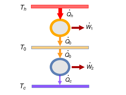
Figure 1: Two autonomous heat engines tightly coupled via a third heat reservoir at temperature $T_{0}$, which satisfies $T_{c}\leq T_{0}\leq T_{h}$. The total power output is $\dot{W}=\dot{W}_{1}+\dot{W}_{2}$.

In this paper, we analyse the global performance of two autonomous heat engines which are tightly coupled via a third heat reservoir having a temperature intermediate between the hot and cold reservoirs (see Fig. 1). Within a linear-irreversible framework, we optimize the total power output and show that EMP is bounded as $\eta^{*}\leq{\eta_{\rm C}}\left({1+{T_{c}}/{T_{0}}}\right)^{-1}$, where the upper bound is achieved under strong coupling (SC) condition. The previous bound of $\eta_{\rm C}/2$ is recovered for $T_{0}=T_{c}$, but can be breached for $T_{0}>T_{c}$ . Further, the requirement that EMP depends only on the ratio $T_{c}/T_{h}$, or equivalently upon $\eta_{\rm C}$ [17], requires that $T_{0}$ be expressed as a mean value of the hot and cold temperatures. Interestingly, specific choices of some common means for $T_{0}$ rather lead to well-known expressions for the EMPs of two-reservoir heat engines (Table 1). This also attributes the above mentioned universal features to EMP, if the choice is restricted to the so-called symmetric means. We also derive EMP for sub-optimal coupling and suggest a new universality class for EMP in the case of broken time reversal symmetry (TRS). More precisely, in place of the universal 1/8 coefficient in the series expansion of EMP, we derive a universal coefficient of 6/49 for the case of broken TRS. Finally, apart from the engine, we are able to optimize the cooling power in the refrigerator mode—a goal which proves to be elusive in some of the previously studied models.

Mean	$T_{0}\equiv{\cal M}(T_{h},T_{c})$	$\eta_{u}^{*}=\eta_{\rm C}\left({1+\frac{T_{c}}{T_{0}}}\right)^{-1}$	Physical model
Geometric	$\sqrt{T_{h}T_{c}}$	$1-\sqrt{1-\eta_{\rm C}}$	Ref. [3]
Harmonic	$\dfrac{2T_{h}T_{c}}{T_{h}+T_{c}}$	$\dfrac{2\eta_{\rm C}}{4-\eta_{\rm C}}$	Refs. [4, 5, 11, 18]
Arithmetic	$\dfrac{T_{h}+T_{c}}{2}$	$\dfrac{(2-\eta_{\rm C})\eta_{\rm C}}{4-3\eta_{\rm C}}$	Ref. [19]
Logarithmic	$\dfrac{T_{h}-T_{c}}{\ln T_{h}-\ln T_{c}}$	$\dfrac{\eta_{\rm C}^{2}}{\eta_{\rm C}-(1-\eta_{\rm C})\ln(1-\eta_{\rm C})}$	Refs. [20, 21, 22, 23]
Lehmer	$\dfrac{T_{h}^{\sigma}+T_{c}^{\sigma}}{T_{h}^{\sigma-1}+T_{c}^{\sigma-1}}$	$\dfrac{\eta_{\rm C}}{2-\dfrac{\eta_{\rm C}}{1+(1-\eta_{\rm C})^{\sigma}}}$	$\sigma\in R$, Ref. [24]

Table 1: The intermediate temperature ${T_{0}}$ as some well-known symmetric means of $T_{h}$ and $T_{c}$, and the corresponding upper bound for EMP, $\eta^{*}_{u}$, obtained under strong coupling, where $\eta_{\rm C}=1-T_{c}/T_{h}$. Various finite-time models derive these forms of EMP in the listed references.

Based on Fig. 1, let us now consider the performance of the sub-engines. The reservoirs $T_{h}$ and $T_{0}$ are coupled via an autonomous engine leading to power output $\dot{W}_{1}=\dot{Q}_{h}-\dot{Q}_{0}$, and a rate of entropy generation, $\dot{S}_{1}=-\dot{Q}_{h}/T_{h}+\dot{Q}_{0}/T_{0}$, which can be written as:

$$\dot{S}_{1}=-\frac{\dot{W}_{1}}{T_{0}}+{\dot{Q}_{h}}\left(\frac{1}{T_{0}}-\frac{1}{T_{h}}\right).$$ (2)

Similarly, reservoirs $T_{0}$ and $T_{c}$ are coupled via another such engine that leads to power output $\dot{W}_{2}=\dot{Q}_{0}-\dot{Q}_{c}$, and a rate of entropy generation, $\dot{S}_{2}=-\dot{Q}_{0}/T_{0}+\dot{Q}_{c}/T_{c}$, which can be written as:

$$\dot{S}_{2}=-\frac{\dot{W}_{2}}{T_{0}}+{\dot{Q}_{c}}\left(\frac{1}{T_{c}}-\frac{1}{T_{0}}\right).$$ (3)

Since the two sub-engines are tightly coupled with each other, the net heat flux exchanged with the intermediate reservoir is zero. Then, $\dot{W}_{1}+\dot{W}_{2}=\dot{Q}_{h}-\dot{Q}_{c}=\dot{W}$, and $\dot{S}_{1}+\dot{S}_{2}=\dot{S}$ is written as:

$$\dot{S}=-\frac{\dot{W}}{T_{0}}+\dot{Q}_{h}\left(\frac{1}{T_{0}}-\frac{1}{T_{h}}\right)+\dot{Q}_{c}\left(\frac{1}{T_{c}}-\frac{1}{T_{0}}\right).$$ (4)

Let us define: $X_{h}=1/T_{0}-1/T_{h}\geq 0$ and $X_{c}=1/T_{c}-1/T_{0}\geq 0$, so that ${X_{h}+X_{c}}=1/T_{c}-1/T_{h}$. Then, we can write Eq. (4) as

$$\dot{S} =-\frac{\dot{W}}{T_{0}}+\cfrac{\dot{Q}_{h}X_{h}+\dot{Q}_{c}X_{c}}{X_{h}+X_{c}}(X_{h}+X_{c}),$$

$$=-\frac{\dot{W}}{T_{0}}+{\dot{Q}_{\rm av}}\left(\frac{1}{T_{c}}-\frac{1}{T_{h}}\right),$$ (5)

where the average or effective thermal flux is given by

$$\dot{Q}_{\rm av}=(1-\omega)\dot{Q}_{h}+\omega\dot{Q}_{c},$$ (6)

with $\omega=X_{c}/(X_{h}+X_{c})$ satisfying $0\leq\omega\leq 1$. In standard approaches, the reference reservoir is usually chosen to be the coldest reservoir available, and so $T_{0}=T_{c}$. Within the present framework, the reference reservoir is an additional resource at $T_{0}$ and the relevant thermal flux is the average value $\dot{Q}_{\rm av}$. Finally, the total power flux is given as: $\dot{W}=F\dot{x}$, where $F$ is the load and $\dot{x}\equiv\dot{x}_{1}+\dot{x}_{2}$ is the total rate of displacement generated.

Now, assuming a linear-irreversible description at the level of global performance of the coupled engines, we identify the following flux-force pairs:

$${J}_{1} =\dot{x},\qquad X_{1}=-\frac{F}{T_{0}},$$ (7)

$${J}_{2} =\dot{Q}_{\rm av},\quad X_{2}=\frac{1}{T_{c}}-\frac{1}{T_{h}},$$ (8)

so that the rate of entropy production is cast in a bilinear form $\dot{S}=\sum_{i=1}^{2}{J}_{i}X_{i}$. Secondly, the linear regime implies the flux-force relations of the form: $J_{i}=\sum_{j=1}^{2}L_{ij}X_{j}$, where $i=1,2$. Here, the phenomenological coefficients $L_{ij}$ are assumed fixed due to the small magnitudes of the forces. Then, the second-law inequality imposes the following conditions:

$$L_{11},L_{22}\geq 0,\qquad 4L_{11}L_{22}\geq{\left(L_{12}+L_{21}\right)^{2}}.$$ (9)

We first assume the principle of microscopic time-reversal symmetry (TRS) which allows the use of Onsager reciprocity relation: $L_{21}=L_{12}$. In this case, the third inequality above reduces to $L_{11}L_{22}\geq L_{12}^{2}$. This makes it convenient to define a measure, $q=L_{12}/\sqrt{L_{11}L_{22}}$, for the coupling strength between thermodynamic forces, which satisfies: $-1\leq q\leq+1$.

So, the constitutive relations for the fluxes in Eqs. (7) and (8) can be written in the following form.

$$\dot{x} =-{L}_{11}\frac{F}{T_{0}}+{L}_{12}X_{2},$$ (10)

$$\dot{Q}_{\rm av} =-{L}_{12}\frac{F}{T_{0}}+{L}_{22}X_{2}.$$ (11)

From (6) and (11), we can derive the following relations:

$$\dot{Q}_{h} =-{L}_{12}\frac{F}{T_{0}}+{L}_{22}X_{2}+\omega\dot{W},$$ (12)

$$\dot{Q}_{c} =-{L}_{12}\frac{F}{T_{0}}+{L}_{22}X_{2}-(1-\omega)\dot{W}.$$ (13)

Optimization of power output: By using Eq. (10), we optimize the power output, $\dot{W}=F\dot{x}$, with respect to the load $F$. The optimal load is obtained at $F^{*}=L_{12}T_{0}X_{2}/2L_{11}$. The optimal power, $\dot{W}^{*}\equiv\dot{W}(F^{*})$, is given by:

$$\dot{W}^{*}=\frac{L_{12}^{2}T_{0}X_{2}^{2}}{4L_{11}}.$$ (14)

Similarly, the hot flux, $\dot{Q}^{*}_{h}\equiv\dot{Q}_{h}(F^{*})$, is obtained from Eq. (12) as:

$$\dot{Q}_{h}^{*}=\left[1+\frac{q^{2}}{4}\left(\frac{T_{0}}{T_{c}}-3\right)\right]L_{22}X_{2}.$$ (15)

Then, the efficiency at maximum power (EMP), $\eta^{*}=\dot{W}^{*}/{\dot{Q}_{h}}^{*}$, is evaluated to be:

$$\eta^{*}={\eta_{\rm C}}\left[{1+\left(\frac{4-2q^{2}}{q^{2}}-1\right)\frac{T_{c}}{T_{0}}}\right]^{-1}.$$ (16)

For given reservoir temperatures, the EMP can be varied by tuning the coupling strength $q$, but it remains bounded as:

$$0\leq\eta^{*}\leq{\eta_{\rm C}}\left({1+\frac{T_{c}}{T_{0}}}\right)^{-1}\equiv\eta_{u}^{*}$$ (17)

where the upper bound is saturated for strong coupling ($q^{2}=1$).

Next, we address universal properties of EMP in the context of our coupled model. The previous studies on universality of EMP were mostly carried out on two-reservoir set ups, where EMP is obtained as a function of $T_{c}/T_{h}$. In the present model, with three reservoirs, the EMP depends on two ratios involving three temperatures, as in Eq. (16). Now, $T_{0}$ may be assigned some numerical value in the interval $[T_{c},T_{h}]$. However, as we show in the following, when $T_{0}$ is expressed as an algebraic mean of $T_{h}$ and $T_{c}$, then the EMP depends only on $T_{c}/T_{h}$ and we can establish a comparison with the EMP of two-reservoir models.

Let ${\cal M}(a,b)$ define an algebraic mean of two real numbers $a,b>0$, which satisfies $\text{min}[a,b]<{\cal M}(a,b)<\text{max}[a,b]$. So, we define ${\cal M}(a,a)=a$. Further, ${\cal M}$ is a homogeneous function of its arguments, satisfying ${\cal M}(\lambda a,\lambda b)=\lambda{\cal M}(a,b)$, for all real $\lambda$. Thus, we can write ${\cal M}(a,b)=a{\cal M}(1,b/a)$. Assuming $T_{0}$ to be such a mean of hot and cold temperatures, i.e. $T_{0}\equiv{\cal M}(T_{h},T_{c})$, we can write: $T_{0}\equiv T_{h}{\cal M}(1,T_{c}/T_{h})=T_{h}{\cal M}(1,1-\eta_{\rm C})$. In other words, $\eta^{*}$ of Eq. (16 ) becomes a function only of $\eta_{\rm C}$, or the ratio of cold to hot temperatures.

Then, for a small difference between the hot and cold temperatures ($\eta_{\rm C}$ as small parameter), we may develop ${\cal M}$ as a Taylor series in $(-\eta_{\rm C})$:

$${\cal M}(1,1-\eta_{\rm C})=1+a_{1}(-\eta_{\rm C})+a_{2}(-\eta_{\rm C})^{2}+{\cal O}[\eta_{\rm C}^{3}],$$ (18)

where the coefficients $a_{1},a_{2},...$ are determined by the form of the given mean [25]. The corresponding series expansion of Eq. (16) is then given by:

$$\eta^{*}=\frac{q^{2}}{4-2q^{2}}\eta_{\rm C}+(1-a_{1})\frac{(4-3q^{2})q^{2}}{(4-2q^{2})^{2}}\eta_{\rm C}^{2}+{\cal O}[\eta_{\rm C}^{3}].$$ (19)

The first order term above is the same as for a two-reservoirs (hot and cold) set up [2], being independent of the intermediate temperature $T_{0}$. For $q^{2}=1$, this term yields the half-Carnot value. The coefficient of the second-order term depends on $q^{2}$ as well as on $a_{1}$ which is a characteristic of the mean $T_{0}$ (see Eq. (18)). Remarkably, if $T_{0}$ is a symmetric mean, i.e. having the property ${\cal M}(T_{h},T_{c})={\cal M}(T_{c},T_{h})$, then $a_{1}=1/2$ [26], and we may rewrite Eq. (19) as:

$$\eta^{*}=\beta\eta_{\rm C}+\frac{\beta(1-\beta)}{2}\eta_{\rm C}^{2}+{\cal O}[\eta_{\rm C}^{3}],$$ (20)

where $\beta\equiv{q^{2}}/{(4-2q^{2})}$ and $0\leq\beta\leq 1/2$. Thus, we have a universal relation between the first and second order coefficients, which is valid for any choice of the symmetric mean $T_{0}$. In particular, for models with SC, $\beta=1/2$, and thus we obtain 1/8 as the second-order coefficient, analogous to the two-reservoirs case [13].

Interestingly, many known expressions for EMP can be derived by assigning a specific mean to $T_{0}$. The few examples of Table I pertain to the scenario $q^{2}=1$, for which Eq. (16) yields $\eta^{*}=\eta_{\rm C}\left({1+{T_{c}}/{T_{0}}}\right)^{-1}$. Upon comparison between this formula and a known expression for EMP, the corresponding $T_{0}$ may be inferred.

As another example, a tandem construction of linear-irreversible engines [2] leads to the EMP, $\eta^{*}=1-(1-\eta_{C})^{\beta}$. Comparing this expression for EMP with Eq. (16), we obtain:

$$T_{0}=\cfrac{\beta-1}{\beta}\;\cfrac{T_{h}^{\beta}-T_{c}^{\beta}}{T_{h}^{\beta-1}-T_{c}^{\beta-1}},$$ (21)

a special case of the generalized mean [27, 28]. Due to $0\leq\beta\leq 1/2$, $T_{0}$ is bounded as: $T_{h}T_{c}/T_{\rm L}\leq T_{0}\leq\sqrt{T_{h}T_{c}}$, with $T_{\rm L}=(T_{h}-T_{c})/\log(T_{h}/T_{c})$ as the logarithmic mean. Here, CA-efficiency [3] is obtained with $\beta=1/2$, for which $T_{0}=\sqrt{T_{h}T_{c}}$.

Further, it is not hard to find examples of asymmetric means, ${\cal M}(T_{h},T_{c})\neq{\cal M}(T_{c},T_{h})$, that can parametrize more general expressions of EMP. Thus, the use of weighted harmonic mean: $T_{0}={T_{h}T_{c}}/[(1-\alpha)T_{h}+\alpha T_{c}]$ in Eq. (16) yields $\eta^{*}={\eta_{\rm C}}/({2-\alpha\eta_{\rm C}})$, where $0\leq\alpha\leq 1$. The symmetric case of $\alpha=1/2$ has been already mentioned in Table 1. The above expression has been derived in various models, where, for instance, the parameter $\alpha$ may quantify the ratio of heat transfer coefficients [4] or dissipation constants [11, 15] on the hot and cold sides of the engine.

The basic framework can be easily generalized to scenarios with a broken TRS, for which the reciprocity relation is no longer true, i.e. $L_{21}\neq L_{12}$. Then, the second flux-force relation, Eq. (11), reads as: $\dot{Q}_{\rm av}=-{L}_{21}{F}/{T_{0}}+{L}_{22}X_{2}$. Following an analogous derivation as for the time-symmetric case, the EMP is given as:

$$\eta^{*}_{{\cancel{\scriptscriptstyle{\text{ TRS}}}}}={\eta_{\rm C}}\left[{1+\left(\frac{1-{\gamma}}{{\gamma}}\right)\frac{T_{c}}{T_{0}}}\right]^{-1}.$$ (22)

Here, $\gamma\equiv xy/(4+2y)$, with $x=L_{12}/L_{21}$ and $y=L_{12}L_{21}/(L_{11}L_{22}-L_{12}L_{21})$ [8]. For $x=1$, we can write $y=q^{2}/(1-q^{2})$ or $\gamma=\beta$, and so Eq. (22) reduces to Eq. (16), thus recovering the results of the model satisfying TRS. Secondly, note that for $T_{0}=T_{c}$, results of the previous studies [8, 9] are recovered, by which $\eta^{*}_{{\cancel{\scriptscriptstyle{\text{ TRS}}}}}=\gamma\eta_{\rm C}$. Thus, the presence of an additional reservoir at $T_{0}>T_{c}$, raises the EMP beyond $\gamma\eta_{\rm C}$.

As noted in Refs. [8, 9], for a given value of $x$, the parameter $\gamma$ lies in the range: $0\leq\gamma\leq x^{2}/(4x^{2}-6x+4)\equiv\hat{\gamma}$. Since the EMP of Eq. (22) is a monotonic increasing function of $\gamma$, so the optimal EMP is given by:

$$\eta^{*}_{{\cancel{\scriptscriptstyle{\text{ TRS}}}}}=\eta_{\rm C}\left[1+\frac{1-\hat{\gamma}}{\hat{\gamma}}\cfrac{T_{c}}{T_{0}}\right]^{-1}.$$ (23)

Clearly, for $x=1$, we obtain $\hat{\gamma}=1/2$, recovering the results of the strong-coupling case, $\eta^{*}=\eta_{\rm C}/(1+T_{c}/T_{0})$. Fig. 2 plots Eq. (23) for different special cases. As argued in Ref. [9], the upper bound of EMP can be breached in the case of broken TRS, yielding the optimal EMP as $4\eta_{\rm C}/7(>\eta_{\rm C}/2)$. It is apparent from Fig. 2 that the intermediate temperature $T_{0}$ helps to go beyond this result too and so the bound $4\eta_{\rm C}/7$ is rendered just as the lower bound.

Although the exact expression for EMP depends on the specific form of $T_{0}$, we can inquire into the universal features just as for the case with TRS. For an arbitrary symmetric mean $T_{0}$, and in proximity to equilibrium, we get

$$\eta^{*}_{{\cancel{\scriptscriptstyle{\text{ TRS}}}}}=\gamma\eta_{C}+\frac{\gamma(1-\gamma)}{2}\eta_{C}^{2}+{\cal O}[\eta_{\rm C}^{3}].$$ (24)

The above series generalizes Eq. (20) which is obtained with $x=1$, for which $\gamma=\beta$. For the case of optimal EMP where $\hat{\gamma}=4/7$ ($x=4/3$ [9]), the series expansion (24) is given by:

$$\eta^{*}_{\cancel{{\scriptscriptstyle{\text{TRS}}}}}=\frac{4}{7}\eta_{\rm C}+\frac{6}{49}\eta_{\rm C}^{2}+{\cal O}[\eta_{\rm C}^{3}].$$ (25)

Thus, corresponding to $\{1/2,1/8\}\equiv\{4/8,6/48\}$ pair of universal coefficients for optimal EMP in the time-symmetric case, we obtain $\{4/7,6/49\}$ as the corresponding universal pair in the case of broken TRS.

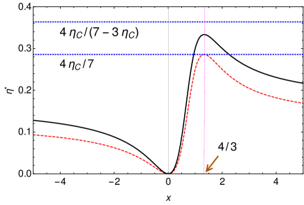
Figure 2: The (red) dashed curve denotes EMP for $T_{0}=T_{c}$ whose optimal value is $4\eta_{\rm C}/7$, obtained at $x=4/3$ [9]. For $T_{c}\leq T_{0}\leq T_{h}$, the optimal EMP is bounded between the two dashed horizontal lines, and is able to breach the $4\eta_{\rm C}/7$ value. The thick (black) curve is the EMP for $T_{0}=(T_{h}+T_{c})/2$, which is also optimal at $x=4/3$.

Model of coupled refrigerators: By reversing the energy flows in Fig. 1, we can study two tightly coupled refrigerators in a similar manner. In this case, it is possible to optimize cooling power of the total machine, as we show below.

We can write the total rate of entropy generation as:

$$\dot{S} =\frac{\dot{W}}{T_{0}}-{\dot{Q}_{\rm av}}\left(\frac{1}{T_{c}}-\frac{1}{T_{h}}\right).$$ (26)

Then, we identify the following flux-force pairs:

$${J}_{1} =\dot{x},\qquad X_{1}=\frac{F}{T_{0}},$$ (27)

$${J}_{2} =\dot{Q}_{\rm av},\quad X_{2}=-\left(\frac{1}{T_{c}}-\frac{1}{T_{h}}\right),$$ (28)

so that $\dot{S}$ is cast in a bilinear form, $\dot{S}\equiv{J}_{1}X_{1}+{J}_{2}X_{2}$.

Within the linear-irreversible framework, the fluxes in Eqs. (27) and (28) take the following form:

$$\dot{x} ={L}_{11}\frac{F}{T_{0}}+{L}_{12}X_{2}$$ (29)

$$\dot{Q}_{\rm av} ={L}_{12}\frac{F}{T_{0}}+{L}_{22}X_{2}$$ (30)

Then, we can derive the following relations:

$$\dot{Q}_{h} ={L}_{12}\frac{F}{T_{0}}+{L}_{22}X_{2}+\omega\dot{W},$$ (31)

$$\dot{Q}_{c} ={L}_{12}\frac{F}{T_{0}}+{L}_{22}X_{2}-(1-\omega)\dot{W}.$$ (32)

Maximum cooling power: We maximize the cooling power, by setting

$$\frac{\partial\dot{Q}_{c}}{\partial F}=0.$$ (33)

The optimal value of $F\equiv\hat{F}$ is given by:

$$\hat{F}=\frac{L_{12}X_{2}T_{0}(2T_{h}-T_{0})}{2L_{11}(T_{0}-T_{h})}.$$ (34)

The coefficient of performance (COP) of the refrigerator at maximum cooling power is defined as:

$$\xi^{*}=\frac{\dot{Q}_{c}(\hat{F})}{\dot{W}(\hat{F})},$$ (35)

and is evaluated to be:

$$\xi^{*}=\frac{(1-t_{0})}{t_{0}^{2}(2-t_{0})}\left[(2-t_{0})^{2}-\frac{4(1-t_{0})}{q^{2}}\right],$$ (36)

where $t_{0}=T_{0}/T_{h}$. For a given $q$ value, $\xi^{*}$ is a monotonic decreasing function of $t_{0}$. So, the bounds of $\xi^{*}$ are given as:

$$0\leq\xi^{*}\leq\frac{1}{\xi_{\rm C}(2+\xi_{\rm C})}\left[{(2+\xi_{\rm C})^{2}-\frac{4(1+\xi_{\rm C})}{q^{2}}}\right],$$ (37)

where $\xi_{\rm C}=T_{c}/(T_{h}-T_{c})$ is the Carnot bound for COP. For models with SC, Eq. (36) gets simplified to: $\xi^{*}=\xi_{\rm C}(1-t_{0})/(2-t_{0})$, with the bounds as: $0\leq\xi^{*}\leq\xi_{\rm C}/(2+\xi_{\rm C})$.

Concluding, we have studied the global performance of two tightly coupled engines within a three-reservoirs set up. Assuming a linear-irreversible description where the total rate of entropy generation is defined in terms of a weighted average of the hot and cold fluxes, we have optimized the total power and analysed the properties of the corresponding efficiency at maximum power. The EMP, in general, depends on two ratios involving the three reservoir temperatures. However, an interesting simplification occurs if the third temperature is chosen as an algebraic mean between the hot and cold temperatures. In this situation, the EMP can be expressed in terms of the Carnot efficiency of the total set up, or equivalently, the ratio of cold to hot temperatures. Further, the choice of this mean in the form of some common means (such as geometric mean, harmonic mean and so on) yields well-known expressions for EMP found in previous studies on two-reservoir set ups. Similarly, the universal properties of EMP found in the latter case can also be identified in the three-reservoir scenario, when the third temperature is a symmetric mean of hot and cold temperatures.

Finally, universal features of EMP, surprising as they are, may be looked upon as a signature of the universality of thermodynamic approach. The present framework for the global performance of coupled machines provides an effective parameter in $T_{0}$ which may be tuned to obtain EMP in a desired form, thus bringing various mathematical forms of EMP under one formalism. Such an approach, apart from providing a unified viewpoint, can be instrumental in predicting novel features such as the 6/49 second-order coefficient for EMP in the case of broken TRS. The generality of thermodynamics deems it feasible that these features may be observed in systems with broken TRS, such as thermoelectric machines placed in an external magnetic field.

References

- Onsager [1931] L. Onsager, Reciprocal relations in irreversible processes. i., Phys. Rev. 37, 405 (1931).
- Van den Broeck [2005] C. Van den Broeck, Thermodynamic efficiency at maximum power, Phys. Rev. Lett. 95, 190602 (2005).
- Curzon and Ahlborn [1975] F. L. Curzon and B. Ahlborn, Efficiency of a Carnot engine at maximum power output, Am. J. Phys. 43, 22 (1975).
- Chen and Yan [1989] L. Chen and Z. Yan, The effect of heat‐transfer law on performance of a two‐heat‐source endoreversible cycle, J. Chem. Phys. 90, 3740 (1989).
- Schmiedl and Seifert [2008] T. Schmiedl and U. Seifert, Efficiency at maximum power: An analytically solvable model for stochastic heat engines, EPL (Europhysics Letters) 81, 20003 (2008).
- Esposito et al. [2010a] M. Esposito, R. Kawai, K. Lindenberg, and C. Van den Broeck, Efficiency at maximum power of low-dissipation carnot engines, Phys. Rev. Lett. 105, 150603 (2010a).
- Moreau et al. [2012] M. Moreau, B. Gaveau, and L. S. Schulman, Efficiency of a thermodynamic motor at maximum power, Phys. Rev. E 85, 021129 (2012).
- Benenti et al. [2011] G. Benenti, K. Saito, and G. Casati, Thermodynamic bounds on efficiency for systems with broken time-reversal symmetry, Phys. Rev. Lett. 106, 230602 (2011).
- Brandner et al. [2013] K. Brandner, K. Saito, and U. Seifert, Strong bounds on onsager coefficients and efficiency for three-terminal thermoelectric transport in a magnetic field, Phys. Rev. Lett. 110, 070603 (2013).
- Izumida and Okuda [2012] Y. Izumida and K. Okuda, Efficiency at maximum power of minimally nonlinear irreversible heat engines, EPL (Europhysics Letters) 97, 10004 (2012).
- den Broeck [2013] C. V. den Broeck, Efficiency at maximum power in the low-dissipation limit, EPL (Europhysics Letters) 101, 10006 (2013).
- Johal [2018] R. S. Johal, Global linear-irreversible principle for optimization in finite-time thermodynamics, EPL (Europhysics Letters) 121, 50009 (2018).
- Esposito et al. [2009] M. Esposito, K. Lindenberg, and C. Van den Broeck, Universality of efficiency at maximum power, Phys. Rev. Lett. 102, 130602 (2009).
- Esposito et al. [2010b] M. Esposito, R. Kawai, K. Lindenberg, and C. Van den Broeck, Quantum-dot Carnot engine at maximum power, Phys. Rev. E 81 (2010b).
- Johal [2019] R. S. Johal, Performance optimization of low-dissipation thermal machines revisited, Phys. Rev. E 100, 052101 (2019).
- [16] An effective thermodynamic approach was studied for finite-time discrete heat engines by one of the authors in Ref. [12].
- [17] As the two engines are tightly coupled to each other, so the efficiencies of the first and the second engines are related to the global efficiency as, . Thus, is still a measure for the maximal efficiency of the global system, which is achieved when both engines run reversibly.
- Johal and Rai [2016] R. S. Johal and R. Rai, Near-equilibrium universality and bounds on efficiency in quasi-static regime with finite source and sink, EPL (Europhysics Letters) 113, 10006 (2016).
- Singh and Johal [2018] V. Singh and R. S. Johal, Feynman–Smoluchowski engine at high temperatures and the role of constraints, J. Stat. Mech. 2018, 073205 (2018).
- Tu [2008] Z. C. Tu, Efficiency at maximum power of Feynman’s ratchet as a heat engine, J. Phys. A: Math. and Theor. 41, 312003 (2008).
- Van den Broeck and Lindenberg [2012] C. Van den Broeck and K. Lindenberg, Efficiency at maximum power for classical particle transport, Phys. Rev. E 86, 041144 (2012).
- Wang et al. [2013] R. Wang, J. Wang, J. He, and Y. Ma, Efficiency at maximum power of a heat engine working with a two-level atomic system, Phys. Rev. E 87, 042119 (2013).
- Erdman et al. [2017] P. A. Erdman, F. Mazza, R. Bosisio, G. Benenti, R. Fazio, and F. Taddei, Thermoelectric properties of an interacting quantum dot based heat engine, Phys. Rev. B 95, 245432 (2017).
- Cavina et al. [2017] V. Cavina, A. Mari, and V. Giovannetti, Slow dynamics and thermodynamics of open quantum systems, Phys. Rev. Lett. 119, 050601 (2017).
- [25] For example, if , a weighted harmonic mean (), then , so that , , and so on.
-
[26]
Many well-known means are symmetric means, such as
arithmetic mean , geometric mean ,
and harmonic mean . Further, these means
satisfy the following property:
which implies .(38) - Stolarsky [1975] K. B. Stolarsky, Generalizations of the logarithmic mean, Mathematics Magazine 48, 87 (1975).
- Leach and Sholander [1978] E. B. Leach and M. C. Sholander, Extended mean values, The American Mathematical Monthly 85, 84 (1978).