Non-parametric data-driven background modelling using conditional probabilities

Abstract

Background modelling is one of the main challenges in particle physics data analysis. Commonly employed strategies include the use of simulated events of the background processes, and the fitting of parametric background models to the observed data. However, reliable simulations are not always available or may be extremely costly to produce. As a result, in many cases uncertainties associated with the accuracy or sample size of the simulation are the limiting factor in the analysis sensitivity. At the same time, parametric models are limited by the a priori unknown functional form and parameter values of the background distribution. These issues become ever more pressing when large datasets become available, as it is already the case at the CERN Large Hadron Collider, and when studying exclusive signatures involving hadronic backgrounds.

A widely applicable approach for non-parametric data-driven background modelling is proposed, which addresses these issues for a broad class of searches and measurements. It relies on a relaxed version of the event selection to estimate conditional probability density functions and two different techniques are discussed for its realisation. The first relies on ancestral sampling and uses data from a relaxed event selection to estimate a graph of conditional probability density functions of the variables used in the analysis, while accounting for significant correlations. A background model is then generated from events drawn from this graph, on which the full event selection is applied. In the second, a novel generative adversarial network is trained to estimate the joint probability density function of the variables used in the analysis. The training is performed on a relaxed event selection, which excludes the signal region, and the network is conditioned on a blinding variable. Subsequently, the conditional probability density function is interpolated into the signal region to model the background. The application of each method on a benchmark analysis and on ensemble tests is presented in detail, and the performance is discussed.

1 Introduction

The modelling of background processes is a critical element in determining the discovery potential of hadron collider experiments searching for physics beyond the Standard Model (SM). In this direction, data-driven background estimation methods have been deployed. In simple cases, it is sufficient to estimate the expected number of background events in a given signal region, for example through single or double sideband methods. But in most cases, reliable description of the background shape in a discriminant variable is also required. For these cases, background modelling often relies on direct simulation based on Monte Carlo (MC) event generators or on parametric methods.

In many physics analyses, however, the dominant contribution to the total background cannot be modelled with sufficient accuracy using MC simulations. Typical examples include fully hadronic final states and backgrounds associated with the mis-identification of physics objects at the reconstruction level. Furthermore, the composition of the background itself, in terms of distinct scattering processes, may not be reliably known. This can lead to a situation where the characteristics of the total background cannot be accurately predicted, even if some of the known components can be modelled with sufficient accuracy.

In the case of parametric methods, the shape of the background in the variable of interest is interpolated, or less often extrapolated, using a functional form modelling the underlying background distribution. The parameters of the function are obtained directly from a fit to the data. Challenges associated with this approach include identifying the optimal functional form: a function with too many free parameters will result in a reduced statistical power, while one with too few parameters may not have enough flexibility to describe the underlying distribution. Fundamentally, however, there is no guarantee that the actual distribution of the background is part of the family of curves parameterised by the chosen function. This may directly bias the extraction of a potential signal. Several approaches have been devised to quantify the potential bias associated with this issue. One such approach is to perform “spurious-signal” calculations ATLAS:2012yve ; ATLAS:2020fzp , which rely on computationally intensive MC simulations. Another approach involves discrete profiling of an ensemble of parametric forms Dauncey:2014xga ; CMS:2020xrn ; CMS:2020xwi , including a penalty factor to account for differences in the number of free parameters. This penalty factor needs, in principle, to be determined in a case-by-case basis, considering coverage properties and any residual bias. A further complication arises in the presence of correlated uncertainties across different event categories, where although the application of the method is conceptually simple, in practice approximations are required. It is noted, that the modeling of smooth backgrounds with non-parametric methods has also been proposed, for example through Gaussian Processes Frate:2017mai .

In this article, a widely applicable approach for non-parametric data-driven background modelling is proposed to derive a reliable understanding of the background to searches for physics beyond the SM in decays of the Higgs boson. It is general enough to be applicable to a broad spectrum of analyses, including both searches and precision measurements, and utilises directly a relaxed version of the event selection to estimate conditional probability density functions. Two different techniques are discussed for its realisation: the first, based on the concept of ancestral sampling, is demonstrated within the context of a search for rare exclusive hadronic decays of the Higgs boson Aaboud:2017xnb ; Aaboud:2018txb ; Aaboud:2016rug ; Aad:2015sda , while the second, based on novel generative adversarial networks, is demonstrated within the context of a search for Higgs boson decays to a $Z$ boson and an undiscovered light resonance, decaying to a low-multiplicity hadronic final state Aad:2020hzm .

The two case studies presented here are analysed using separate samples of simulated signal and background events. The event generator configuration specific to the $H\to\phi\gamma$ search is described in section 2.2 while the corresponding configuration for the search for $H\to Za\to\mu\mu+{\rm jet}$ is described in section 3.2. For both channels, generated events are processed with the Delphes fast simulation framework (version 3.4.2) deFavereau:2013fsa . This framework uses parameterised descriptions of the response of collider experiment detectors to provide reconstructed physics objects, enabling a realistic data analysis to be performed. As an example of a general purpose Large Hadron Collider (LHC) detector, the ATLAS-like configuration card included in Delphes is used. This is minimally modified to use the charged hadron tracking resolution from the earlier version 3.3.3, which was found to more closely reproduce the performance of the LHC general purpose detectors CMS:2014pgm . The effect of multiple $pp$ interactions in the same or neighbouring bunch crossings (pileup) are not simulated, since it represents a negligible contribution to the background in both case studies.

In both implementations, a generative model is derived that aims to reproduce the kinematic and related event selection variables that are subsequently used to model a compound variable of interest, for example the invariant mass of the system. Conditional probabilities have also been employed for background parameterisation through density estimation Mathad:2019rqj ; Nachman:2020lpy . Typically, the density estimate is obtained from the sidebands and is interpolated (or extrapolated) to the signal region, while it is made conditional to one or more variables of interest. Furthermore, in an earlier work Andreassen:2020nkr the “deep neural networks using classification for tuning and reweighting” procedure Andreassen:2019nnm was used to reweight a background simulation in the sideband of a resonant feature of the potential signal. The training of the neural network was conditional on that feature variable, which enables the subsequent interpolation to the signal region.

2 Background modelling with ancestral sampling

Consider a hypothetical particle $X$, decaying to a multi-body final state. In order to establish the existence of such a hypothetical particle within a dataset, one typically begins by identifying candidate decay products within an event and studying the distribution of compound kinematic variables of the reconstructed system. When studying the distributions of such compound kinematic variables, typically the invariant mass, for evidence of a new particle, an accurate description of these distributions for the background is a primary ingredient in the statistical analysis and interpretation of the observed events.

The method outlined in this article, based on the concept of ancestral sampling Goodfellow-et-al-2016 , centres around a construct termed a “kernel”. The kernel represents a description of the distributions and correlations among a set of variables, which include the components of the four vectors, possibly in addition to other quantities, such as an isolation measure, of each of the reconstructed decay products. From this kernel, a data structure termed a “pseudo-candidate” can be randomly sampled, such that an ensemble of pseudo-candidates will respect both the distributions of, and correlations among, the same variables in the data sample used to build the kernel.

In the simplest case of the two-body decay $X\to ab$, where only the four vectors of decay products $a$ and $b$ are described, the most general form of the kernel is an eight dimensional distribution of the four vector components of the two decay products. Given that the method is designed to be built from a dataset, such as a sample of data events collected by a collider experiment, the kernel may be an eight dimensional histogram built from the source dataset.

Histograms of dimensionality in excess of three are often not practical. It is therefore necessary, in order to limit the impact of statistical fluctuations, to minimise the dimensionality of the kernel. It is often possible to substantially reduce the dimensionality of the kernel through a judicious choice of the variables used and a good understanding of the correlations among them. An ideal choice is one that minimises the number of strong correlations among variables. In such a case, the description of the kernel can be factorised from a single distribution of high dimensionality into multiple distributions of low dimensionality. In this way, only the most important correlations among variables are explicitly described, while the remaining small correlations are effectively removed. The extent of this factorisation can be chosen based on the accuracy required and the size of the dataset available to build the kernel.

Once the kernel has been established, an ensemble of pseudo-candidates can be generated. Each pseudo-candidate is built by randomly sampling values from each of the factorised distributions in a sequential manner. Compound kinematic quantities for each pseudo-candidate, such as the invariant mass or transverse momentum of the system of two decay products, can be calculated on a per-candidate basis; this forms the basis upon which a model describing the distribution of compound kinematic quantities is derived.

2.1 Overview of case study: search for $H\to\phi(K^{+}K^{-})\gamma$

The coupling of the Higgs boson to the first and second generation fermions is yet to be confirmed experimentally. Rare exclusive decays of the Higgs boson into a light meson and a photon have been suggested as a probe of the couplings of the Higgs boson to light quarks. Specifically, the Higgs boson decay into a $\phi$ meson, where the decay $\phi\to K^{+}K^{-}$ is considered, and a photon is sensitive to the Higgs boson coupling to the strange quark. The ATLAS collaboration has performed a search for such decays using a dataset corresponding to $36\,\text{fb}^{-1}$ of $\sqrt{s}=13\,\text{TeV}$ $pp$ collisions Aaboud:2017xnb . The final state consists of a pair of oppositely charged kaons, with an invariant mass consistent with the $\phi$ meson mass, recoiling against an isolated photon. The main sources of background in this search are events involving inclusive direct photon production or multijet processes where a meson candidate is reconstructed from charged particles produced in a hadronic jet. Such processes are difficult to model accurately with MC event generators and represent an ideal use case for a data-driven non-parametric background modelling method. The ancestral sampling-based technique described in this paper has been successfully deployed in several ATLAS searches for radiative Higgs boson decays to light mesons Aaboud:2017xnb ; Aaboud:2018txb ; Aaboud:2016rug ; Aad:2015sda . In this paper the original technique and a modified implementation are presented, their statistical properties are characterised, and their relationship is discussed.

2.2 Event selection, analysis strategy and simulation

The event selection used in this case study closely follows that described in ref. Aaboud:2017xnb . Events are required to contain a photon with transverse momentum, $p_{\text{T}}(\gamma)$, in excess of $35\,\text{Ge\kern-1.00006ptV}$, and pseudorapidity, $\eta(\gamma)$, within $|\eta(\gamma)|<2.37$. Photon candidates with pseudorapidity in the transition region between barrel and endcap calorimeter regions, $1.37<|\eta(\gamma)|<1.52$, are excluded. Candidate $\phi\to K^{+}K^{-}$ decays are reconstructed from pairs of oppositely charged tracks with transverse momentum, $p_{\text{T}}(K)$, in excess of $15\,\text{Ge\kern-1.00006ptV}$, and absolute pseudorapidity, $|\eta(K)|$, less than $2.5$. Furthermore, the highest transverse momentum track within a pair is required to satisfy $p_{\text{T}}(K)>20\,\text{Ge\kern-1.00006ptV}$. These $p_{\text{T}}$ requirements reflect standard trigger thresholds employed in searches for such decay topologies. The invariant mass of track pairs is required to be within the range $1.012<m(\phi)<1.028\,\text{Ge\kern-1.00006ptV}$, which accounts for the resolution of the detector. The $H\to\phi\gamma$ candidate is formed from the combination of the photon with the highest transverse momentum and the $\phi\to K^{+}K^{-}$ candidate with an invariant mass closest to the $\phi$ meson mass. The variable $I(\phi)$ characterises the hadronic isolation of the $\phi\to K^{+}K^{-}$ candidates. $I(\phi)$ is defined as the scalar sum of the $p_{\text{T}}$ of tracks within $\Delta R=\sqrt{\Delta\Phi^{2}+\Delta\eta^{2}}=0.2$, where $\Phi$ is the azimuthal angle, of the leading track within a $\phi\to K^{+}K^{-}$ meson candidate, relative to the transverse momentum of the $\phi\to K^{+}K^{-}$ candidate. The tracks constituting the $\phi$ meson candidate are excluded from the sum. Events are retained for further analysis if $\Delta\Phi(\phi,\gamma)>\pi/2$ and $I(\phi)<0.5$, targeting isolated $\phi$ meson candidates and decay products that are created back-to-back. The transverse momentum of the $\phi$ meson candidate is required to be greater than a threshold that varies as a function of the invariant mass $m_{\phi\gamma}$ of the three-body system. Thresholds of $40\,\text{Ge\kern-1.00006ptV}$ and $47.2\,\text{Ge\kern-1.00006ptV}$ are imposed on $p_{\text{T}}(\phi)$ for the regions $m_{\phi\gamma}<91\,\text{Ge\kern-1.00006ptV}$ and $m_{\phi\gamma}\geq 140\,\text{Ge\kern-1.00006ptV}$, respectively. The threshold is varied from $40\,\text{Ge\kern-1.00006ptV}$ to $47.2\,\text{Ge\kern-1.00006ptV}$ as a linear function of $m_{\phi\gamma}$ in the region $91\leq m_{\phi\gamma}<140\,\text{Ge\kern-1.00006ptV}$. This selection was optimised for a simultaneous search for Higgs and Z bosons decaying to $\phi\,\gamma$. This set of criteria define the “Signal Region” (SR) requirements. $H\to\phi\gamma$ signal events are discriminated from background events by means of a statistical analysis of the distribution of the invariant mass $m(\phi,\gamma)$ of selected candidates.

For the purpose of demonstrating the ancestral sampling background modelling method, only the dominant contributions to the signal and background processes are explicitly simulated. This choice has no implications for the validation of the method and is pragmatically motivated. Inclusive Higgs boson production in $pp$ collisions is approximated by the gluon-fusion process alone and simulated with the Pythia 8.244 MC event generator Sjostrand:2014zea with the CT14nlo PDF set Dulat:2015mca . Subleading contributions from the vector boson fusion process and Higgs boson production in association with vector bosons and heavy quarks are not simulated explicitly. The $H\to\phi\,\gamma$ decay is simulated directly by the Pythia 8.244 MC event generator Sjostrand:2014zea and no other Higgs boson decays are simulated. The $\gamma+\text{jet}$ process alone is used as a proxy for the inclusive background to the $H\to\phi\gamma$ search, which is expected to also contain contributions from multijet events. The production of $\gamma+\text{jet}$ is simulated with the Sherpa 2.2.10 event generator Gleisberg:2008ta with the NNPDF3.0 PDF set NNPDF:2014otw . Direct photon production with up to two additional jets is simulated at the matrix element level. The simulated $\gamma+\text{jet}$ sample contains around $3\times 10^{8}$ unweighted events and corresponds to an effective integrated luminosity of around $20\,\text{fb}^{-1}$.

2.3 Overview of method

The procedure is based on a sample of data events selected based on the nominal “Signal Region” requirements described in section 2.2, modified by relaxing a number of criteria in order to enrich the sample in background events. The criteria which define this background-dominated sample are denoted the “Generation Region” (GR). Two additional event samples, known as “Validation Regions” (VR), are also defined to validate the background modelling procedure. The VR event samples are non mutually exclusive subsets of the GR sample and the definitions of these regions are outlined in table 1.

	Minimum $p_{\text{T}}(\phi)$ requirement	Maximum $I(\phi)$ requirement
GR	$35\,\text{Ge\kern-1.00006ptV}$	Not applied
VR1	Varying from 40 to $47.2\,\text{Ge\kern-1.00006ptV}$	Not applied
VR2	$35\,\text{Ge\kern-1.00006ptV}$	0.5
SR	Varying from 40 to $47.2\,\text{Ge\kern-1.00006ptV}$	0.5

Table 1: The event selection criteria of the “Signal Region” which are modified to define the "Generation Region" and "Validation Regions".

These $n$ events in the GR are used to construct probability density functions of the relevant kinematic and isolation variables, parameterised to respect the most important correlations. This can be achieved either by directly utilising each of the $n$ events once, as in refs. Aaboud:2017xnb ; Aaboud:2018txb ; Aaboud:2016rug ; Aad:2015sda , or by sampling $n$ events from the GR dataset with replacement. These approaches are found to produce background models of equal accuracy, as outlined in section 2.10. In the case study that follows, results from the former are presented and comparisons to the latter are made where relevant differences occur.

By sampling the obtained distributions, an ensemble of $H\to\phi\gamma$ pseudo-candidates is generated, from which a model of the $m(\phi,\gamma)$ distribution for background events can be derived for the SR requirements. In addition to providing a prediction for the shape of the $m(\phi,\gamma)$ distribution, the normalisation of the SR and VRs, relative to the GR, is also predicted. The absolute normalisation in the SR and VRs may be obtained directly by the model, by uniformly scaling the distributions by the ratio of the number of data events in the GR to the size of the ensemble of pseudocandidates.

2.4 Sampling procedure

Each pseudo-candidate event is described by $\phi$ and $\gamma$ four-momentum vectors and an associated $\phi$ hadronic isolation variable, $I(\phi)$. The generation templates which together parameterise all components of the $\phi$ and $\gamma$ four-momentum vectors and the $\phi$ hadronic isolation variable are described in table 2 and represented in figure 1.

Template Name	Dimensionality	Variable 1	Variable 2	Variable 3
A	2D	$p_{\text{T}}(\phi)$	$p_{\text{T}}(\gamma)$	-
B	3D	$\Delta\Phi(\phi,\gamma)$	$p_{\text{T}}(\gamma)$	$p_{\text{T}}(\phi)$
C	2D	$\Delta\eta(\phi,\gamma)$	$\Delta\Phi(\phi,\gamma)$	-
D	2D	$I(\phi)$	$p_{\text{T}}(\gamma)$	-
E	1D	$\eta(\gamma)$	-	-
F	1D	$\Phi(\gamma)$	-	-
G	1D	$m(\phi)$	-	-

Table 2: The definition of the set of generation templates from which the components of the pseudo-candidates are sequentially sampled.

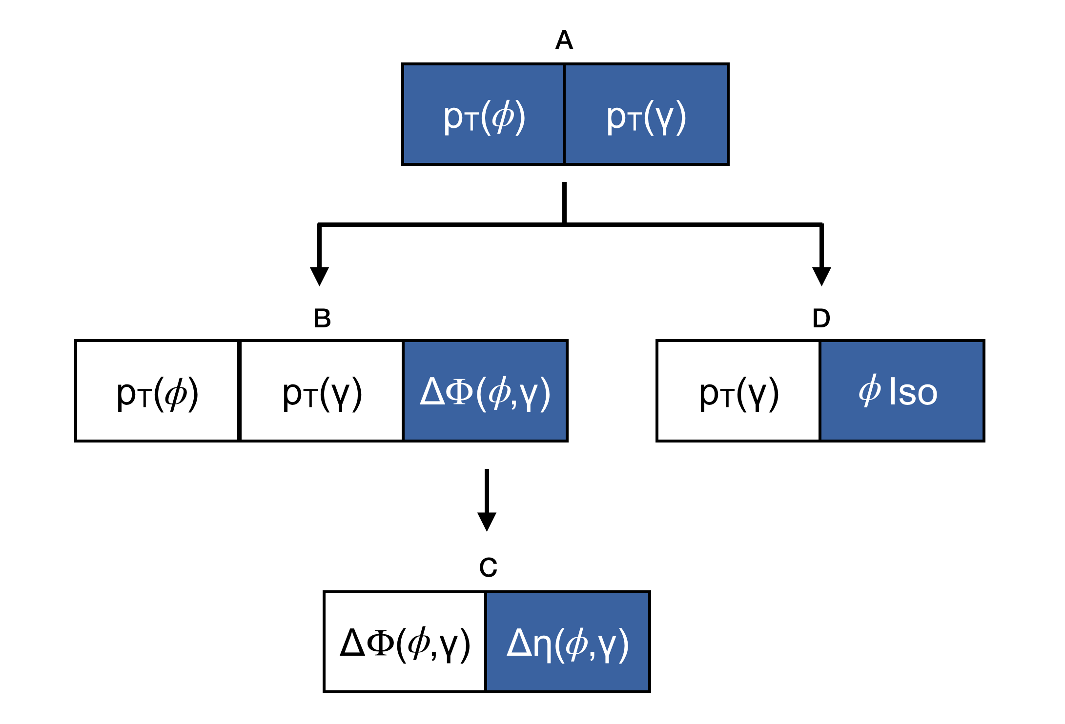
Figure 1: Graphical representation of the sampling sequence followed in the modelling. Variables not shown explicitly are sampled in a factorised, uncorrelated, manner from an 1D template, as described in table 2.

The sampling procedure for a single pseudo-candidate proceeds as follows:

1. Correlated values for $p_{\text{T}}(\phi)$ and $p_{\text{T}}(\gamma)$ are sampled from generation template A.

2. Based on the values of $p_{\text{T}}(\phi)$ and $p_{\text{T}}(\gamma)$ sampled in step 1, template B is projected along the $\Delta\Phi(\phi,\gamma)$ dimension and a value for $\Delta\Phi(\phi,\gamma)$ is sampled.

3. Based on the value of $\Delta\Phi(\phi,\gamma)$ sampled in step 2, template C is projected along the $\Delta\eta(\phi,\gamma)$ dimension and a value for $\Delta\eta(\phi,\gamma)$ is sampled.

4. Based on the value of $p_{\text{T}}(\gamma)$ sampled in step 1, template D is projected along the $I(\phi)$ dimension and a value is sampled.

5. Values for $\eta(\gamma)$ and $\phi(\gamma)$ are sampled from generation templates E and F, respectively. At this stage, the photon four-momentum is fully defined, with $m(\gamma)=0$ imposed.

6. A value for $m(\phi)$ is sampled from generation template G. At this stage, the $\phi$ four-momentum is fully defined.

The steps above are repeated to generate an ensemble of pseudo-candidates whose characteristics resemble those of the GR data sample. The selection requirements of the SR and two VR are imposed on the ensemble and the pseudo-candidates which are retained are used to construct distributions of composite variables built from the $\phi$ and $\gamma$ four-momentum, of which $m(\phi,\gamma)$ is of primary interest.

2.5 Validation

Both the distributions and correlations of important primary and composite variables are validated by comparing the ensemble of pseudo-candidates to the data sample. Figure 2 shows the $m(\phi,\gamma)$ distribution of the data sample and sample of pseudo-candidates for the GR, VR1, VR2 and SR selection criteria, respectively. Accounting for event weighting, the GR contains 30175 events, while the SR contains 11885 events. The modelling of the kinematic and isolation variables in the SR, for the data sample and the sample of pseudo-candidates in the SR is presented in figure 3. The accurate reproduction of composite variables relies on the correlations among variables to be adequately described in the ensemble of pseudo-candidates, which in turn is determined by the sampling procedure and parameterisation of generation templates. Figures 2 and 3 exhibit very good agreement between the sample of pseudo-candidates and data events for both the $m(\phi,\gamma)$ and $p_{\text{T}}(\phi,\gamma)$ distributions, indicating that the important correlations in the data sample are well modelled by the sample of pseudo-candidates. Linear correlation coefficients, evaluated between each of the important variables, are shown in figure 4 for both the data sample and ensemble of pseudo-candidates. Both the hierarchy and general magnitude of the correlation coefficients in the data are well reproduced by the model.

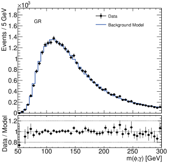
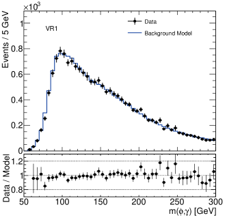
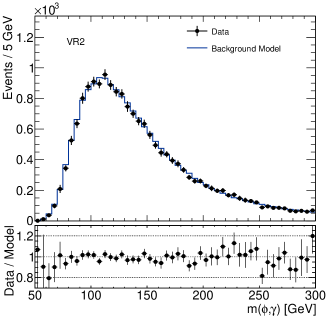
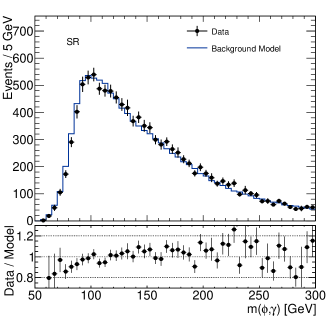
Figure 2: $m(\phi,\gamma)$ distributions in the GR, VR1, VR2 and SR for the simulated data and background model.

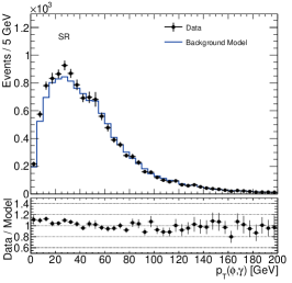
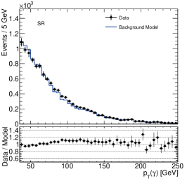
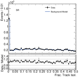
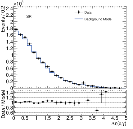
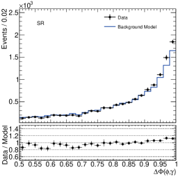
Figure 3: Distributions of kinematic and isolation variables in the SR, for the simulated data and background model.

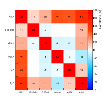
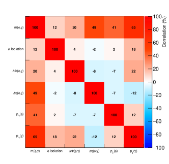
Figure 4: Linear correlation coefficients for pairs of variables used in the background modelling procedure, shown for the simulated data events (left) and generated pseudo-candidates (right) passing the GR selections.

2.6 Signal injection tests

While the GR dataset is defined such that it is dominated by background events, a small contribution from signal events, relative to the background, may be present. In the limit that the signal to background ratio in the GR becomes large, one can intuitively expect that the reliability of the method will begin to degrade. In order to quantify what level of signal contribution must be present in the GR in order to induce a noticeable impact on the reliability of the model, signal injection tests are performed. Specifically, it is estimated that a signal contribution in the GR of approximately 130 events, would correspond to a statistical significance of 5.5 standard deviations in the SR. Consequently, 130 signal events were injected into the GR dataset and the background model was re-derived. Figure 5 shows a comparison of the model constructed with and without this signal injection. The total background prediction between $122.5<m(\phi,\gamma)<127.5\,\text{Ge\kern-1.00006ptV}$ in the SR increases by approximately 2%. The outcome of this signal injection test demonstrates that the method is robust against the presence of even a large, in terms of corresponding statistical significance in the SR, signal contributions to the GR dataset. Furthermore, the effect on the background is found to scale linearly with the number of injected signal events.

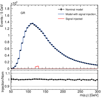
(a)

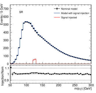
(b)

Figure 5: Comparison of the $m(\phi,\gamma)$ distributions predicted by the model for 5(a) the GR and 5(b) the SR, derived with and without an injection of approximately 130 $H\to\phi\,\gamma$ signal events in the GR dataset.

2.7 Systematic uncertainties

While the tests described in section 2.5 demonstrate that the model can provide an accurate description of the background at the level of precision associated with the statistical uncertainty of the validation regions, potential mismodelling beyond this level cannot be directly excluded. It is therefore important that systematic uncertainties affecting the shape of the predicted background distributions are estimated.

The strategy for incorporating systematic uncertainties in the model is motivated by the context within which the model is applied to perform the statistical analysis, namely a likelihood fit. The strategy focuses on estimating a set of complementary background shape variations which are implemented as shape variations of the nominal background probability density function. The derived shape variations are selected to capture different modes of potential deformations of the background shape. The exact size of the variation is of less importance, given that the corresponding nuisance parameters are constrained directly by the data in the likelihood fit. Moreover, the analyser may decide to leave such nuisance parameters completely free, or to add Gaussian constraint terms in the likelihood. In the latter case, care must be taken to ensure that the assigned $\pm 1\sigma$ shape variations are large with respect to potential discrepancies between the shape of the predicted distributions and those in the data.

Pairs of approximately anti-symmetric shape variations are built by performing the sampling procedure after having applied a transformation to one of the generation templates. The transformations considered here include:

• A translation of the photon transverse momentum distribution.

• A multiplicative transformation of the $\Delta\Phi(\phi,\gamma)/\pi$ distribution by a function of the form $1+C\times\Delta\Phi(\phi,\gamma)$, where a pair of values (positive and negative) for the coefficient $C$ are chosen.

Furthermore, additional alternative background models may be derived by direct transformations of the resulting distribution of interest. For example, an additional pair of alternative background models is derived by a multiplicative transformation of SR $m(\phi,\gamma)$ distribution by a linear function of $m(\phi,\gamma)$. These three pairs of shape variations largely span the range of possible large scale uncorrelated shape deformations of the $m(\phi,\gamma)$ distribution, as shown in figure 6.

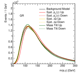
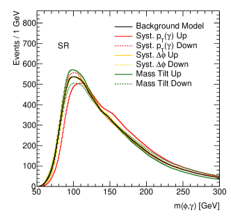
Figure 6: Comparison of the $m(\phi,\gamma)$ distributions for the GR (left) and SR (right) associated with the three pairs of systematic shape variations.

2.8 Treatment of resonant background components

In certain cases, in addition to the dominant backgrounds which do not exhibit resonant structures in the invariant mass distribution, non-negligible resonant contributions may also be present. One such example is the $Z\to\mu^{+}\mu^{-}\gamma$ process, which represents an important resonant background in the case of searches for radiative Higgs boson decays to the $\Upsilon(\to\mu^{+}\mu^{-})$ bottomonium states Aad:2015sda ; Aaboud:2018txb . Often such processes can be described with sufficient accuracy by MC simulations and the use of such simulations to describe these subsets of the overall background is preferable. In this situation, the procedure used to build the kernel is modified, to ensure that such resonant contributions are not included in the model for the inclusive non-resonant background. During the construction of the generation templates, data events in the vicinity of the resonance are randomly discarded, with a probability which describes the likelihood that a data event with a given invariant mass was produced by the resonant process. This probability may be determined, as a function of invariant mass, by subtracting the distribution of the MC prediction for the resonant process from the data distribution. This procedure can mitigate the impact of resonant background contributions to the non-resonant background model Aad:2015sda ; Aaboud:2018txb . In the absence of such a procedure, the prediction of the model in the vicinity of the resonance may be distorted in a manner similar to the signal inject tests discussed in section 2.6.

2.9 Implementation in statistical analysis

The performance of the method in practical terms is demonstrated by implementing the background model within a statistical analysis procedure. A binned maximum likelihood fit is performed to the $m(\phi,\gamma)$ distribution of the simulated $\gamma+\text{jet}$ events used to build the background model alone. The $m(\phi,\gamma)$ distribution of the signal is modelled by a double Gaussian distribution with a single mean (common to both Gaussian components), two width parameters and a parameter describing the relative normalisation of the two Gaussian components. The normalisation of the signal, relative to the number of signal events predicted by the simulation, is controlled by a single free parameter, $\mu_{\text{signal}}$, normalised such that $\mu_{\text{signal}}=1$ corresponds to 50 signal events. The background distribution is built from the background model in terms of a finely binned histogram, with a linear inter-bin interpolation applied. For reference the generated background sample was approximately a factor 300 larger than the GR dataset. The normalisation of the background, relative to the number of events predicted by the model, is determined by a single free parameter, $\mu_{\text{bkgd}}$. Systematic uncertainties affecting the shape of the background model, described in section 2.7, are implemented using a moment morphing technique Baak:2014fta . Each of the three shape variations described in section 2.7 are implemented independently, each being controlled by an individual nuisance parameter. The value of the nuisance parameters describing the $p_{\text{T}}(\gamma)$ shift and $\Delta\Phi(\phi,\gamma)$ deformation are constrained by Gaussian penalty terms in the likelihood, while the $m(\phi,\gamma)$ tilt nuisance parameter is free.

The result of the fit is presented in figure 7, where it is shown that the post-fit background model is in good agreement with the $m(\phi,\gamma)$ distribution of the simulated $\gamma+\text{jet}$ events. The fitted values of the parameters are shown in table 3. As discussed earlier, the post-fit uncertainty of the nuisance parameters indicates the statistical power of the data to constrain the corresponding shape deformations with respect to their pre-fit magnitude. Furthermore, the non-zero post-fit values of the nuisance parameters demonstrate the ability of the background model to absorb potential residual mismodelling effects.

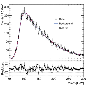
Figure 7: The $m(\phi,\gamma)$ distribution of simulated $\gamma+\text{jet}$ events overlaid with the result of a binned maximum likelihood fit using the method described in section 2 to derive the background PDF.

Parameter	Value	Uncertainty ($\pm 1\sigma$)
$\mu_{\text{signal}}$	$-0.07$	$\pm 0.54$
$\mu_{\text{bkgd}}$	$1.01$	$\pm 0.01$
Shape: $p_{\text{T}}(\gamma)$ shift	$0.26$	$\pm 0.15$
Shape: $\Delta\Phi(\phi,\gamma)$ tilt	$0.30$	$\pm 0.43$
Shape: $m(\phi,\gamma)$ tilt	$0.10$	$\pm 0.24$

Table 3: Post-fit parameter values and their associated uncertainties.

The impact of the systematic uncertainties on the signal strength measurement is quantified through fits in which the nuisance parameters associated with the shape variations are fixed, one at a time, to their best fit values plus or minus their correspond uncertainty. The change in the obtained $\mu_{\text{signal}}$ in each of these fits, expressed in terms of $\sigma_{\mu_{\text{signal}}}$, is shown in table 4.

		$\Delta\mu_{\text{signal}}/\sigma_{\mu_{\text{signal}}}$
Shape: $p_{\text{T}}(\gamma)$ shift	$+1\sigma$	-0.18
	$-1\sigma$	+0.17
Shape: $\Delta\Phi(\phi,\gamma)$ tilt	$+1\sigma$	+0.07
	$-1\sigma$	-0.11
Shape: $m(\phi,\gamma)$ tilt	$+1\sigma$	-0.22
	$-1\sigma$	+0.19

Table 4: The change in the fitted signal strength, relative to its uncertainty, is shown for the case where the corresponding nuisance parameter is fixed to its best fit value plus or minus its corresponding uncertainty.

2.10 Ensemble tests using synthetic datasets

In order to more thoroughly validate the performance of the method in a manner less sensitive to statistical fluctuations, an ensemble of independent statistical tests identical to that described in section 2.9 were performed. For the purposes of these tests, a synthetic dataset sampled from analytic functions was generated in order to simulate an appropriately large number of events on a practical timescale. The form of the analytic functions was chosen to mimic the relevant distributions of the MC simulated events described in section 2.2. Events with a complete four-vector for the $\phi\gamma$ system are generated according to the following procedure:

• A value for $m(\phi,\gamma)$ is sampled from a Landau distribution, whose parameters are chosen to mimic the GR distribution in figure 2

• A value for $p_{\text{T}}(\phi,\gamma)$ is sampled from a Gaussian distribution, whose mean and standard deviation parameters vary as a function of $m(\phi,\gamma)$

• A value for $\eta(\phi,\gamma)$ is sampled from an analytical distribution $f(\eta)=G(\eta,-\mu,\sigma)+G(\eta,\mu,\sigma)$, where $G$ is the Gaussian distribution

• A value for $\Phi(\phi,\gamma)$ is uniformly sampled in the interval $\Phi(\phi,\gamma)\in\{-\pi,\pi\}$

Four-vectors for the $\phi$ (and subsequent $\phi\to K^{+}K^{-}$ decay products) and $\gamma$ are generated by means of kinematic phase space sampling with isotropic angular dependence. Finally, a $\phi$ isolation variable sampled from a linear function of $p_{\text{T}}(\phi)$, chosen to mimic the distribution of the MC simulated events described in section 2.2.

An ensemble of 400 independent background-only samples was generated, each containing around $23,000$ synthetic background events in the GR and $16,000$ events in the SR. The number of synthetic background events in each ensemble was chosen to approximately match the effective statistical power of the background MC sample described in section 2.2.

The background modelling procedure was applied to each dataset in the ensemble and the statistical analysis described in section 2.9 was applied. Two signal masses were considered. For the first, the signal was located on the peak of the rising kinematic edge of the $m(\phi,\gamma)$ distribution. The second was located in the area where the $m(\phi,\gamma)$ distribution is smoothly falling, as in the main case study. The distribution of the signal strength normalised to its uncertainty, also referred to as the pull distribution, for each signal mass hypothesis is shown in figure 8. In each case, the pull distribution is shown for the background model obtained by directly utilising each of the $n$ events in the GR once and for that obtained by sampling $n$ events from the GR dataset with replacement. In all cases, the ensemble tests demonstrate that the method provides a background model of sufficient accuracy to avoid any substantial bias in the statistical quantification of a potential signal. Nevertheless, for the background models obtained by directly utilising once each of the $n$ events in the GR, the width of the pull distribution is substantially less that the expected value of unity. In contrast, for the background model obtained by sampling the GR events with replacement, the width of the pull distribution is much closer to unity.

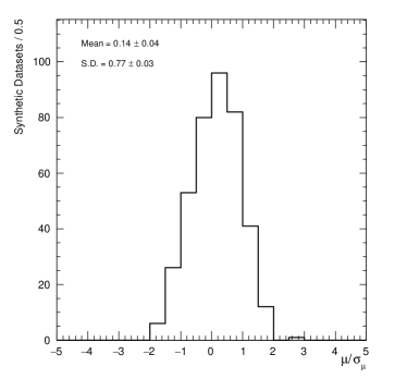
(a)

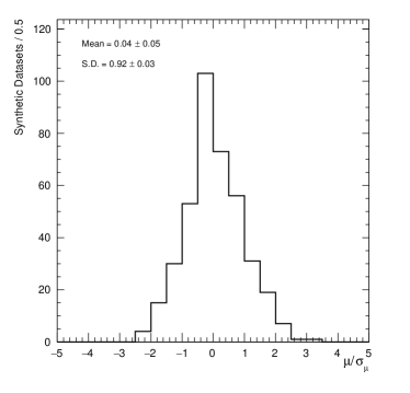
(b)

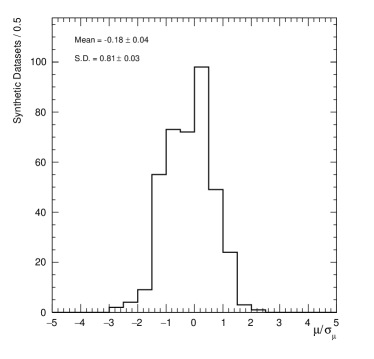
(c)

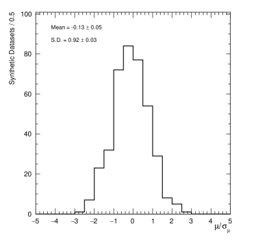
(d)

Figure 8: Ensemble test distributions of fitted signal strength, normalised to uncertainty, for each of the two mass hypotheses considered: 8(a) and 8(b) signal located on kinematic peak of $m(\phi,\gamma)$ distribution, 8(c) and 8(d) signal located on smoothly falling region of $m(\phi,\gamma)$ distribution. In 8(a) and 8(c) the background model is obtained by using once each of the $n$ events in the GR, while in 8(b) and 8(d) the GR is sampled $n$ times.

The observed deviation in the width of the pull distribution from unity arises because the events in the SR are not independent from the events used to obtain the background model, since the SR is a subset of the GR. This is illustrated in figure 9(a) for the case where the background model is obtained utilising each of the $n$ events in the GR once. In this figure, the data and the obtained background model are compared, prior to any fit, for two distinct experiments from the ensemble. It is shown that the background model reproduces the fluctuations in the background shape observed in the specific experiment to a good degree. The size of this effect scales with, $N_{SR}/N_{GR}$, the ratio of the number of events in the SR relative to that of the GR, and is practically removed as this ratio tends to zero. Typically, as in the case of the analyses presented in refs. Aaboud:2017xnb ; Aaboud:2018txb ; Aaboud:2016rug ; Aad:2015sda , this ratio is of order 10% or less. However, such low values may not always be possible to achieve due to experimental limitations. Nevertheless, in such cases, correct statistical coverage can be obtained by means of a MC study.

In cases where an appropriately small value of $N_{SR}/N_{GR}$ cannot be achieved or a MC study is not feasible, this effect is mitigated by deriving the model by sampling $n$ events from the GR dataset with replacement. This is clearly demonstrated in figure 9(b), where the width of the pull distribution is shown as a function of $N_{SR}/N_{GR}$ for each for the implementations. The sampling of the GR with replacement leads to reduced correlations between the fitted dataset and background model, resulting in a pull distribution which is practically compatible with unity.

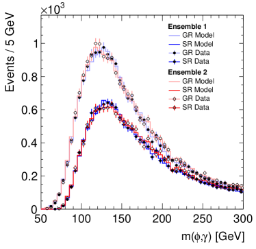
(a)

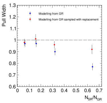
(b)

Figure 9: 9(a) Data and background model comparison for two distinct experiments in the ensemble. The background model is obtained utilising each of the $n$ GR events once. 9(b) The width of the pull distribution for ensemble tests with different SR-to-GR event fractions. The red markers have been shifted by -0.5% along the horizontal axis for visibility.

3 Background modelling with generative adversarial networks

Generative adversarial networks (GANs) Goodfellow:2014upx are generative machine learning algorithms, widely used in image synthesis, see for example refs. radford2015unsupervised ; karras2017progressive ; brock2018large ; zhang2017stackgan ; 9043519 ; YI2019101552 . They consist of a pair of neural networks, as shown in figure 10: the generator, which is trained to learn a generative model from a training data sample; and the discriminator, which is simultaneously trained to discriminate the sample derived from the generative model from the training data sample. The generator is trained to maximise the probability that the discriminator misclassifies the generated events for real data. The use of GANs in high energy physics is an active topic of research, where they can generate events significantly faster than traditional techniques Alanazi:2021grv ; Butter:2020tvl , significantly increasing the effective statistical power of a sample Butter:2020qhk . This speed-up is crucial for big data applications, for example in the HL-LHC, where large simulated datasets are required to match the statistical precision of the data.

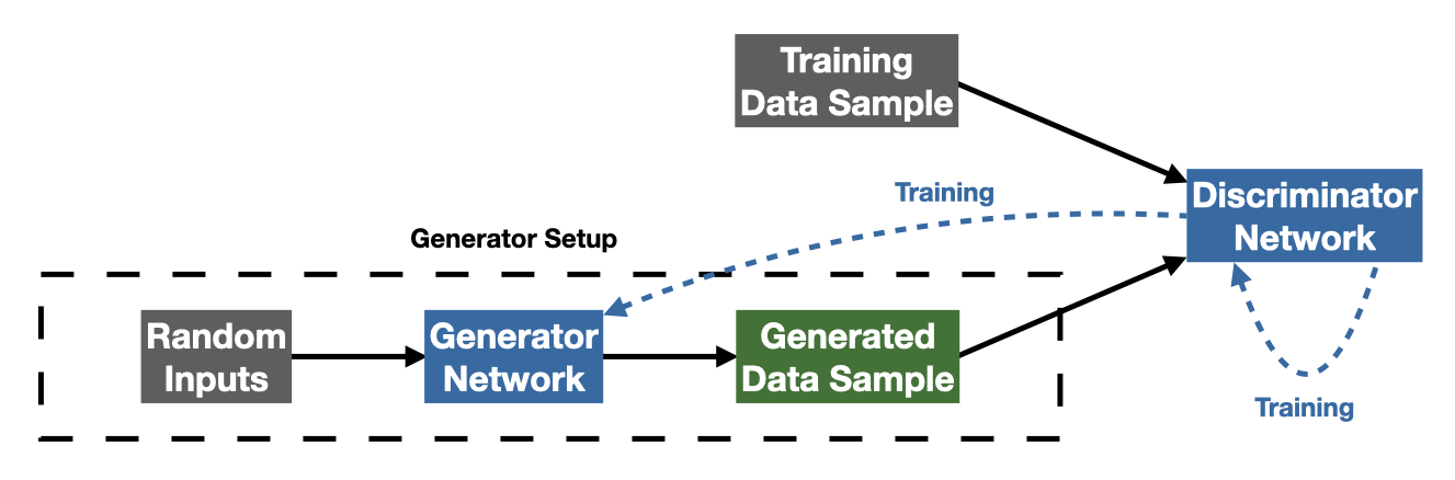
Figure 10: Schematic representation of a generative adversarial network.

In the context of particle physics, where the application of machine learning techniques is ever expanding as demonstrated by recent reviews on the topic Radovic:2018dip ; Guest:2018yhq ; Bourilkov:2019yoi ; Schwartz:2021ftp ; Karagiorgi:2021ngt ; Feickert:2021ajf , the use of GANs has been explored in applications spanning the complete chain of event generation, simulation, and reconstruction. The use of GANs for simulating the hard scattering process was considered in ref. Otten:2019hhl ; Butter:2019cae ; SHiP:2019gcl , while the use of GANs for pileup description and detector simulation was explored in ref. Martinez:2019jlu and Ghosh:2020kkt , respectively. Recent publications have also explored the idea of replacing the entire reconstructed-event generation pipeline with a GAN Otten:2019hhl ; Hashemi:2019fkn ; DiSipio:2019imz ; DiSipio:2019sug ; Farrell:2019fsm ; Alanazi:2020klf ; Vallecorsa:2019ked . Each of these applications differ in the nature of the training data used, but mostly use simulated training datasets. This solves the issue of limited simulated data samples by allowing large generated samples to be produced from much smaller datasets. However, concerns related to simulation-based mismodelling remain, which often result in some of the largest sources of uncertainty in searches and measurements at the LHC.

In our approach, this is resolved by “blinding” the data signal region (SR) while training the GAN. Training a standard GAN using blinded data explicitly, and falsely, informs the GAN that there are no events in the SR, leading to a generative model which predicts an absence of background events in the SR. For this reason, in this article, a conditional GAN (cGAN) Mirza:2014dfp , shown in figure 11, is used to provide a generative model of the conditional probability distribution of the data, given the value of the variable used to blind the dataset. To do this, it is trained to estimate the function that maps the random latent space and the blinding variable onto the distribution of the other feature variables, in a similar way to how standard GANs are trained. Random points in the latent space are then generated and provided to the cGAN alongside the conditioning variable to estimate the other feature variables, and then the original conditioning variable is appended to the list of estimated feature variables. Despite being given no information about the data in the SR, except for the values of the conditioning variable, the predictions of the cGAN can be interpolated or extrapolated into the SR.

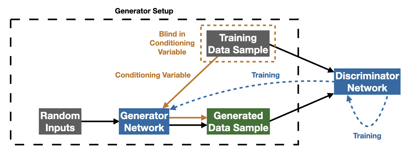
Figure 11: Schematic representation of a conditional generative adversarial network.

To the best of the authors’ knowledge, this cGAN-based technique is the first technique of its kind to be presented. Recently, independently and in parallel to the development of this work, a new approach to anomaly detection in particle physics data analysis was published that also uses a generative model of a conditional probability distribution to model background processes in a SR through interpolation Hallin:2021wme . In that case, the focus is on anomaly detection, rather than for background modelling in a more typical LHC analysis workflow. Furthermore, the generative model is based on neural density estimation through a masked autoregressive flow papamakarios2017masked , as opposed to GANs.

3.1 Overview of case study: search for $H\to Za\to\mu\mu+{\rm jet}$

Searches for additional scalar or pseudo-scalar particles in the Higgs sector are a major part of the LHC physics programme. In particular, the possibility for light pseudo-scalar particles, produced in the decays of the observed Higgs boson, feature in several beyond the SM theories Curtin:2013fra , including the two-Higgs-doublet model (2HDM) and the 2HDM with an additional scalar singlet. Searches typically focus on Higgs boson decays into pairs of the light scalars, or into a $Z$ boson and a light scalar. Several searches have been performed to date, focusing primarily either on masses of the light resonance in excess of $4~{}\text{GeV}$, or considering only leptonic decays of lighter resonances.

Recently, the ATLAS Collaboration published the first search for Higgs boson decays to a $Z$ boson and a light hadronically decaying resonance, $a$  Aad:2020hzm . The $Z$ boson was reconstructed from its leptonic decays to electron pairs and muon pairs ($\ell\ell$). Masses of the light resonance $a$ between $0.5~{}\text{GeV}$ and $4~{}\text{GeV}$ were considered and the hadronic decay of the resonance was reconstructed inclusively as a jet. For event selection, a multilayer perceptron (MLP) Goodfellow-et-al-2016 classifier is employed, which is provided with information related to the resonance mass from a separate MLP-based mass estimator. Finally, following a requirement on the classifier output, an event counting approach was pursued in a mass window of the $\ell\ell\text{j}$ system. The background estimation was performed using a modified version of the ABCD method CDF:1990kbl , where an MC-based correction was used to account for the correlation between the $\ell\ell\text{j}$ system mass and the classifier output.

This is a particularly interesting case study to apply this approach, for two reasons: first, the cross-section of the main background, $Z+\text{jets}$, is such that in the case of a ${\cal O}(100~{}\text{fb}^{-1})$ dataset, it is not feasible to generate a simulated event sample with comparable statistical power. Second, the decaying resonance is identified using multi-variate methods, which require a detailed modelling of a large number of correlations between the relevant kinematic and jet substructure variables. The sensitivity of the published analysis is limited by the background systematic uncertainties, which originate predominantly from the insufficient size of the simulated data samples used. By suppressing these uncertainties, through large background samples derived directly from the data, one may expect to first approximation a fourfold improvement on the obtained 95% confidence level upper limit on the lowest light resonance masses considered, and more significant improvements at higher masses.

In what follows, this analysis is used as a case study to implement a cGAN-based multivariate background modelling method. The study described here is closely aligned with the ATLAS analysis, and the event selection is summarised below. One of the main differences with respect to the ATLAS analysis is that for simplicity only the signal with an $a$ mass of $0.5\,\text{GeV}$ is considered here. Furthermore, in this study, only $Z\to\mu^{+}\mu^{-}$ decays are considered, while the ATLAS analysis also considered $Z\to e^{+}e^{-}$ decays. This practical simplification is inconsequential for the purposes of demonstrating the method.

3.2 Event selection, analysis strategy and simulation

Events are required to contain at least two muons with transverse momenta $p_{\text{T}}>5~{}\text{GeV}$ including an oppositely charged pair, and a hadronic jet with transverse momentum $p_{\text{T}}>20~{}\text{GeV}$, reconstructed using the anti-$k_{t}$ algorithm Cacciari:2008gp ; Cacciari:2011ma with a distance parameter of $0.4$. For events with more than one jet, the jet with the highest $p_{\text{T}}$ is used in the analysis that follows. At least one muon is required to have $p_{\text{T}}>27~{}\text{GeV}$ to model the threshold imposed by the trigger, and the invariant mass of the muons is required to be within $10\,\text{GeV}$ of the $Z$ boson mass.

This selection results in a large background arising from $Z+\text{jets}$ events, which is mitigated using charged particle track-based jet substructure information. Tracks with $\Delta R<0.4$ of the jet are selected if they have $p_{\text{T}}>0.5~{}\text{GeV}$ and if their transverse and longitudinal impact parameters are compatible with the particle being produced at the primary vertex. Events are required to have exactly two tracks passing these requirements. Four substructure variables are formed using these tracks: $\Delta R$ between the highest $p_{\text{T}}$ track and the jet axis; the ratio of the $p_{\text{T}}$ of the highest $p_{\text{T}}$ track to the vector sum of the track $p_{\text{T}}$; angularity (with weight parameter $a=2$) Almeida:2008yp ; and the modified correlation function $U_{1}$ (with an angular exponent $\beta=0.7$) Moult:2016cvt . A neural network is used to separate signal from background events on the basis of substructure variables described above. During the neural network training, only signal events with tracks that originate from the decay of the $a$ are included. A requirement is placed on the output of the MLP which has an efficiency of 96% and 2.5% for $H\to Za$ signal and $Z+\text{jets}$ background events, respectively.

A binned likelihood fit to the invariant mass distribution of the $Z\to\mu^{+}\mu^{-}$ candidate and jet, for events passing this selection, is used to estimate $\sigma(pp\to H)\times\mathcal{B}(H\to Za)$. The signal and mock data are modelled using simulation, and the background is modelled using the cGAN approach. Inclusive Higgs boson production in $pp$ collisions is approximated by the gluon-fusion process alone and simulated with the Pythia 8.244 MC event generator with the CT14nlo PDF set. For the $H\to Za$ search, $Z+\rm{jets}$ production is expected to represent the dominant background. Contributions such as $t\bar{t}$ production are present only at a minor level owing to the requirement of an opposite-charge same-flavour dilepton with an invariant mass consistent with the $Z$ boson mass. For the purposes of this study, the background from $Z+\rm{jets}$ production alone is considered. $Z+\rm{jets}$ production is also simulated with the Pythia 8.244 MC event generator with the CT14nlo PDF set. The simulated $Z+\rm{jets}$ sample contains around $3.5\times 10^{8}$ events and corresponds to an effective integrated luminosity of around $160\,\text{fb}^{-1}$.

3.3 Overview of method

In this method we use a GAN that is trained directly on data. To avoid the risk that the background model is contaminated by potentially present signal events, the SR is “blinded” during the training. For this reason, a cGAN learns a generative model of the data conditional probability distribution, given the value of the blinding variable. The reconstructed invariant mass of a signal is typically a good choice of blinding/conditioning variable for resonant signals where the signal is often localised to a narrow region of the data. Nevertheless, other variables may also be used, and in fact multiple variables may be used at once. Training a standard GAN using blinded data explicitly, and falsely, informs the GAN that there are no events in the SR, leading to a generative model which predicts an absence of background events in the SR. Conversely, the cGAN learns the distribution of the background features conditioned on the blinding variable and so, despite being given no information about the background in the SR, can extrapolate its prediction into the SR. The cGAN can then be provided with the inclusive distribution of the blinding variable for all data events, and use what it learns in the unblinded data to interpolate the conditional generative model into the signal region, thereby predicting the values of the other variables. These variables could, for example, be the inputs to a multivariate classifier. Typically, the inclusive data distribution will often be adequate to model the inclusive distribution of the blinding variable, as the signal contamination is small before the application of a dedicated event selection. In that case, one may input the raw data events directly to cGAN, or they can be used to model the distribution, for example using a standard GAN, a histogram, kernel density estimation, Gaussian Process regression, fitting an analytical function, or any one of a number of other smoothing or modelling techniques.

As a case study, the recently published search for decays of the Higgs boson into a $Z$ boson and a light hadronic resonance is used, where a multivariate classifier is used to target possible BSM signal resonances. Here, the blinding variable is the invariant mass of the $Z$ boson and the light resonance, which peaks at approximately $125~{}\text{GeV}$, the mass of the observed Higgs boson. The variables learnt by the cGAN are four jet substructure variables, largely based on tracking information, which are used as input to a multivariate classifier that is trained for signal to background discrimination. Given an estimate of the inclusive invariant mass distribution, the cGAN then provides estimates of these variables for the background in the SR, from which the output of the classification neural network may be calculated. A requirement on the output of the classifier may then be applied to these generated events, providing an estimate of the background in the SR after the multivariate classification requirement. An extended, binned, profile likelihood fit to the invariant mass distribution of these data events may then be performed using a signal model and the cGAN-based background template, to test for a possible signal.

To demonstrate the performance of the cGAN method, it is used to estimate the substructure variables for the dominant $Z+\text{jets}$ background in the $H\to Za\to\mu\mu\text{j}$ search described above. The cGANs are trained using Keras chollet2015keras with the Tensorflow backend tensorflow2015-whitepaper . Only events with exactly two tracks associated to the jet and $m_{\mu\mu\text{j}}$ in the sidebands of the $m_{\mu\mu\text{j}}$ selection of the SR, $90<m_{\mu\mu\text{j}}<123~{}\text{GeV}$ or $135<m_{\mu\mu\text{j}}<190~{}\text{GeV}$, are used in the cGAN training. Of the events that represent data in this study, 25% are withheld from the cGAN training to quantify the performance of the cGANs. No MLP selection is applied to the events used to train the cGANs. The feature variables are transformed so that they are in the range -1 to 1.

The cGAN generator and discriminator both have architectures of 5 layers of 256 hidden nodes, each with a leaky ReLU activation function with an alpha value of 0.4, and the input space of the generator has 9 latent dimensions and 1 additional dimension for the conditioning variable. Other architectures were tested and were not found to improve the performance. The generator and discriminator are both trained using a binary cross entropy loss function, with an L2 regularisation term for their respective weights. The stochastic gradient descent optimiser is used with Nesterov momentum, and with gradients clipped to a value of 1. The initial network weight values are set using He initialisation, while the biases are initialised to 0. The learning rate and its decay, in addition to the momentum, batch size, and L2 regularisation coefficient are all determined using a random scan over 100 sets of values. The cGANs are trained until no significant gains are obtained.

An ensemble of five cGANs is used to reduce the uncertainty due to imperfections in the cGAN training, which is described in section 3.4. Each cGAN is used to generate 20 times the number of data events that pass the selection, except for the neural network and $m_{\mu\mu\text{j}}$ requirements. The cGANs are evaluated for further training and for inclusion in the ensemble using an analysis-specific $\chi^{2}$-based performance metric. This metric is defined by comparing the data and the prediction of the ensemble in the plane of $m_{\mu\mu\text{j}}$ and the neural network output. Ten bins in $m_{\mu\mu\text{j}}$ for events passing the neural network selection are used, where the total normalisation of the ensemble in this region is set equal to the number of background events in the region. Additionally, in the $m_{\mu\mu\text{j}}$ blinding region the five most signal-like bins in the neural network output are used, where each neural network output region is defined to contain 2.5% of the total data, and the normalisation of the ensemble in each region is corrected by the ratio of the normalisation of the data to the ensemble of the events outside the $m_{\mu\mu\text{j}}$ blinding region. The two most signal like neural network output bins with $123<m_{\mu\mu\text{j}}<135~{}\text{GeV}$ are excluded from the definition of the metric to ensure negligible signal contamination, and that it is uncorrelated to the signal region for events passing the MLP selection and a possible nearby validation region. Only the 25% of events that were withheld from the cGAN training are used in the evaluation of this metric.

3.4 Background modelling uncertainties

Uncertainties with cGAN-based background models can arise due to the interpolation, and imperfect performance of the cGAN. The first source of uncertainty is related to the size of the signal region in the blinding variable, which is determined by the characteristics of the signal. This uncertainty is expected to be smaller for narrower SRs, and for feature variables which vary more slowly across the SR. The second source of uncertainty is related to the quality of the training of the cGAN, which can be improved at the cost of more analyser time or computational power, or with a larger training dataset.

In general, these uncertainties should be quantified on a case-by-case basis, for instance by studying the performance of the derived model in validation regions. A method is provided here, discussed in the context of the case study, which is more broadly applicable. Neglecting the uncertainty due to the interpolation, the remaining reducible uncertainty is then estimated by comparing the predictions of the $m_{\mu\mu\text{j}}$ distributions in the SR of the individual cGANs to that of the ensemble. These uncertainties are correlated between the cGANs, and so a principle component analysis is used to obtain an orthogonal basis.

3.5 Background model validation

The performance of the cGAN is illustrated in figure 12, which shows the substructure variables in the $m_{\mu\mu\text{j}}$ SR. The cGAN is able to model these distributions accurately, despite these data events not being included in the cGAN training. Figure 13 shows the substructure variables for the low and high $m_{\mu\mu\text{j}}$ sidebands separately, demonstrating that the cGAN has successfully learnt the dependence of the substructure variables on $m_{\mu\mu\text{j}}$. The discrepancies at the edges of the distributions are attributed to a number of factors, including: 1. the distributions often having fewer events near the edges, as compared to the cores of the distributions; 2. the edges often being sharply rising or falling; and 3. the fact that the cGAN has fewer nearby events to learn from at the edges of the distributions. Although this is not of importance in the case study presented here, analyses that are sensitive to the modelling at these edges would require a more thorough hyperparameter optimisation and, potentially, a performance metric that places more importance on the quality of modelling in these regions.

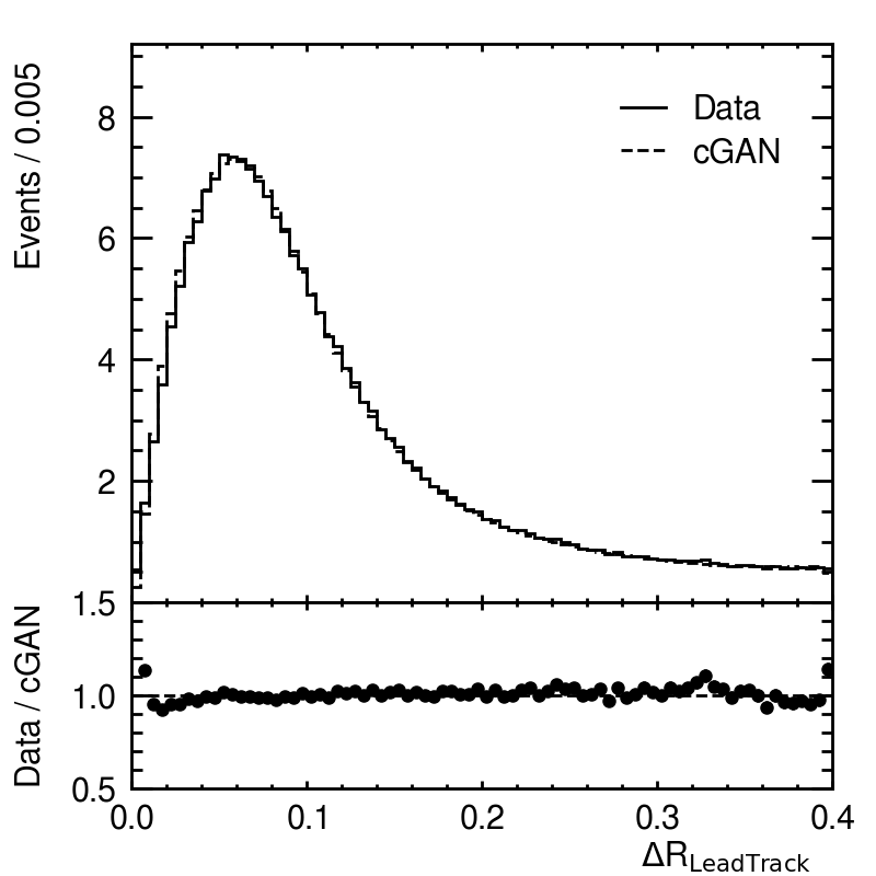
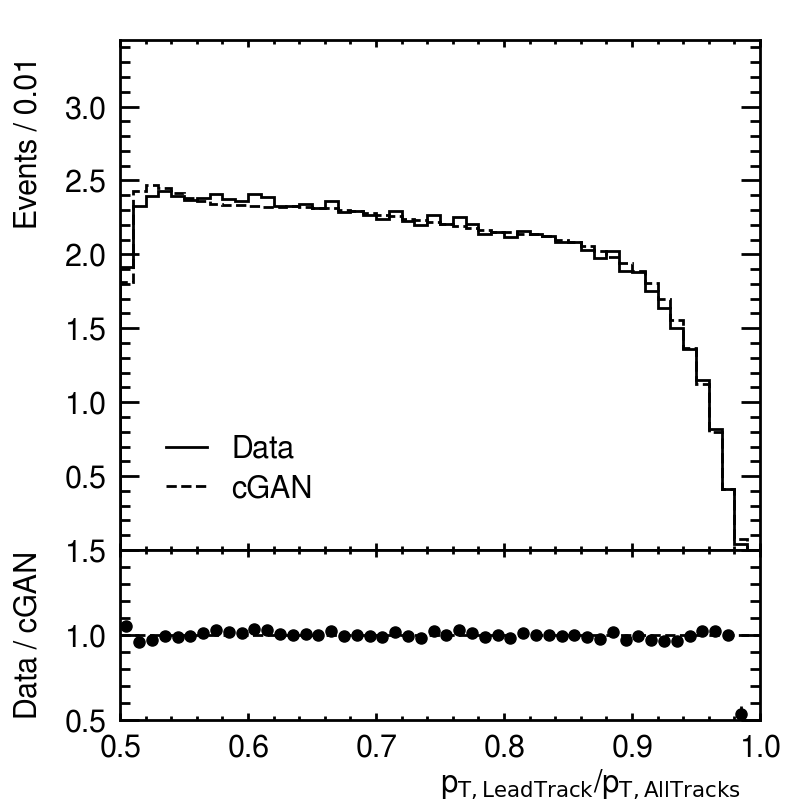
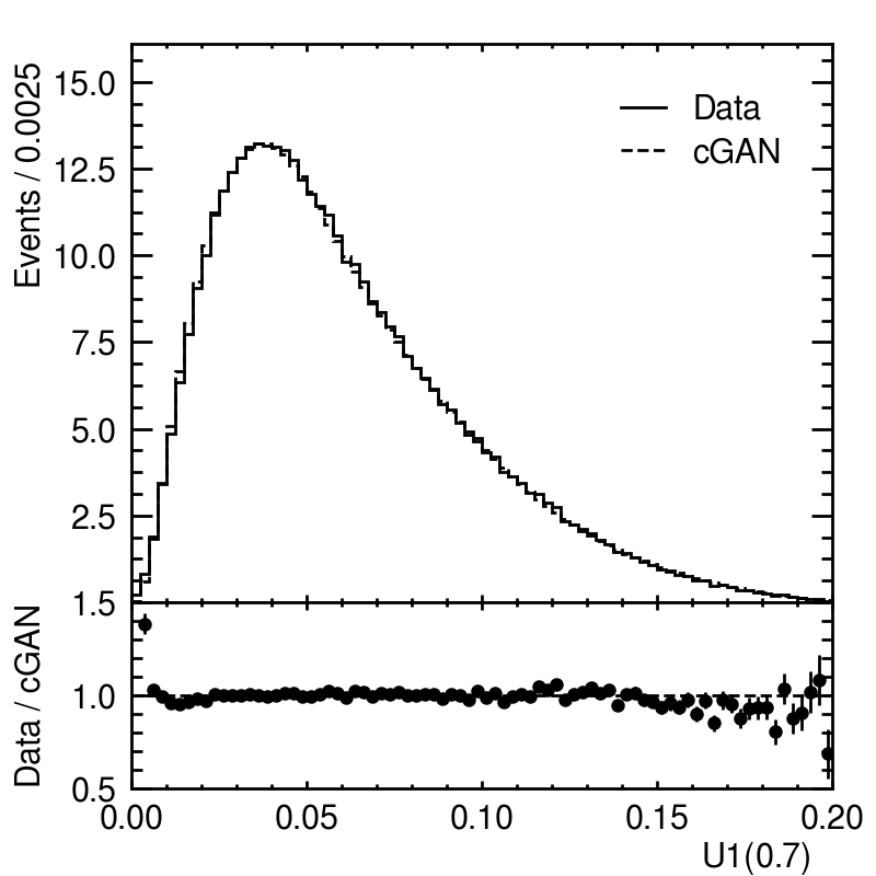
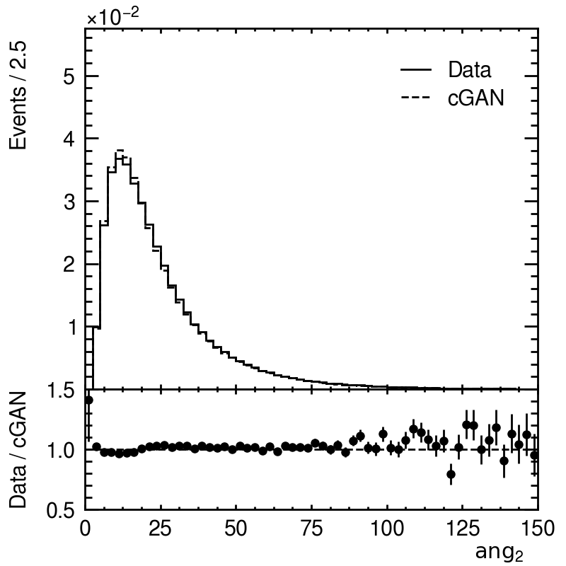
Figure 12: Jet substructure variables in mock data and modelled by the cGAN, which are used as inputs to the classification MLP. The error bars on the markers in the lower panels represent the statistical uncertainty on the mock data.

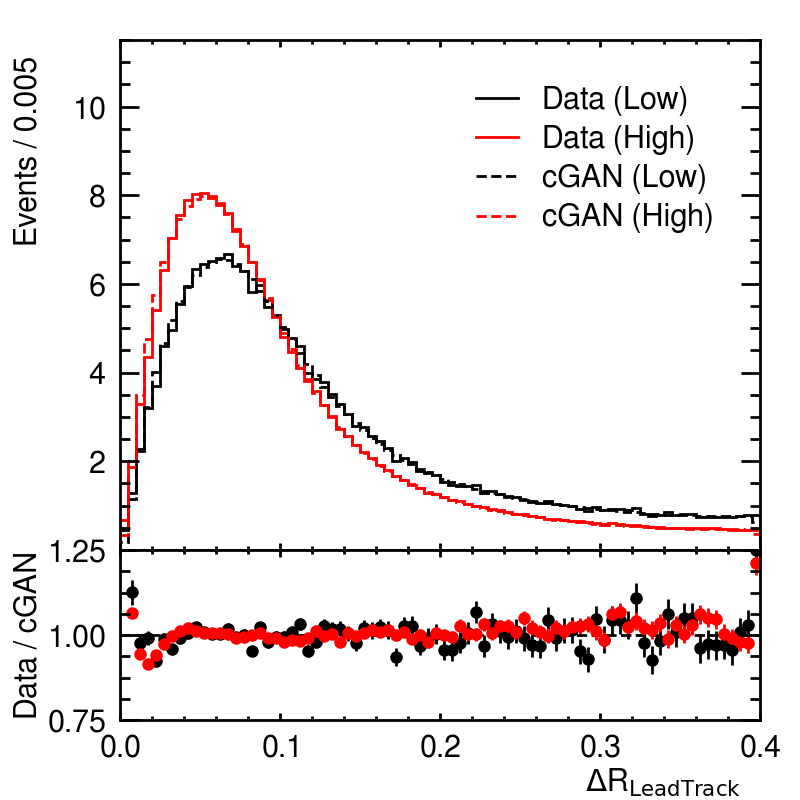
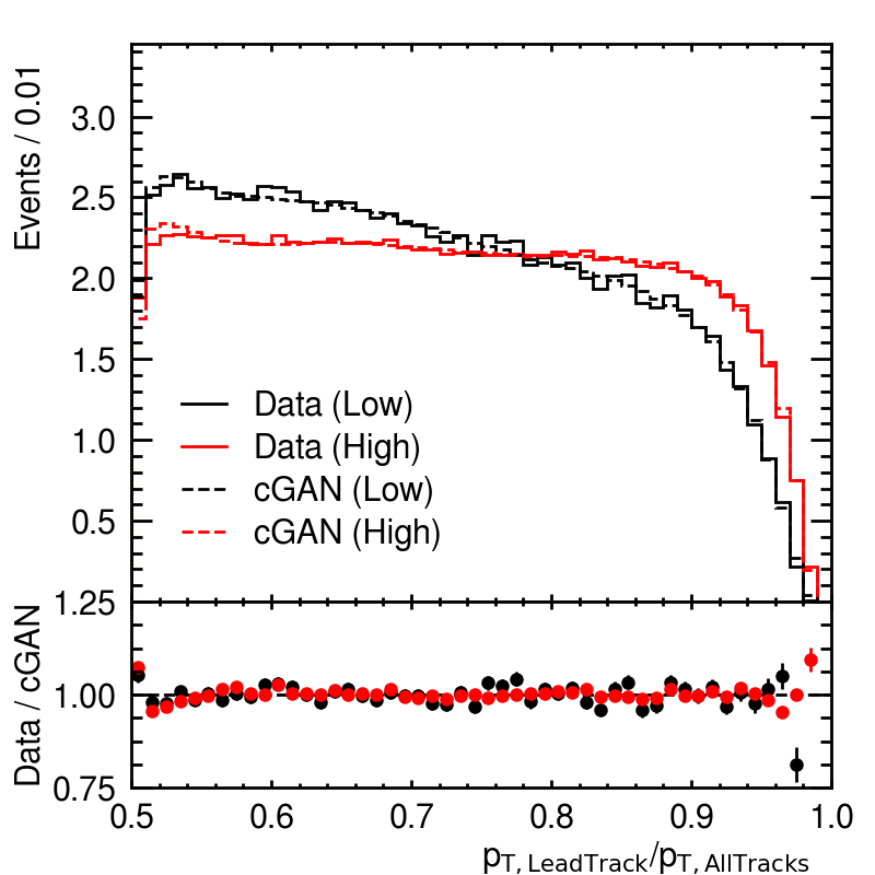
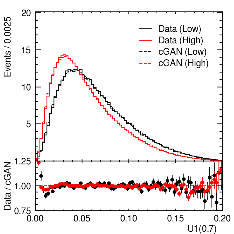
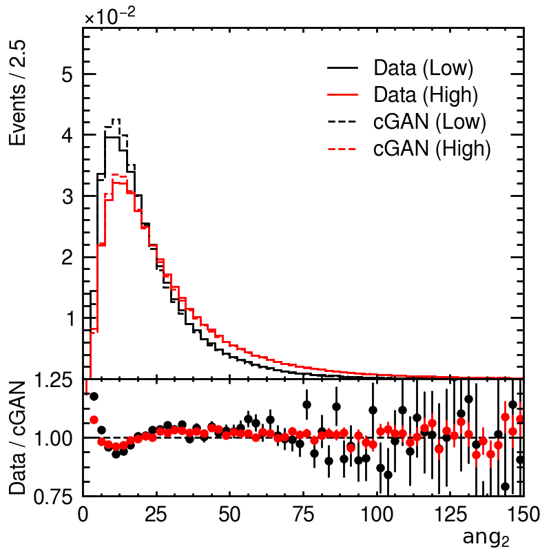
Figure 13: Jet substructure variables in mock data and modelled by the cGAN, which are used as inputs to the classification MLP, shown for the low and high $m_{\mu\mu\text{j}}$ sidebands separately. The error bars on the markers in the lower panels represent the statistical uncertainty on the mock data.

The obtained correlation matrix from the cGAN is compared to the data correlation matrix in figure 14. Excellent agreement is observed. The variation of the top five cGANs about their ensemble is shown in figure 15(a), and the resulting uncertainties from the principle component analysis are shown in figure 15(b).

An extended, binned, profile maximum likelihood fit to the $m_{\mu\mu\text{j}}$ distribution with freely floating signal and background normalisations is used to estimate the signal in the SR from a fit to the background-only dataset. The extracted signal normalisation is $-0.003\pm 0.010$ times its predicted value, assuming a SM Higgs boson cross section LHCHiggsCrossSectionWorkingGroup:2016ypw and a branching fraction $\mathcal{B}(H\to Za)=100\%$. This is compatible with the lack of signal in the dataset used in the fit. The values of all fitted parameters are given in table 5, along with their uncertainties. The $m_{\mu\mu\text{j}}$ distributions after the likelihood fit are shown in figure 16.

This case study demonstrates that the proposed background modelling method is capable of accurately modelling a set of correlated variables, and of interpolating over significant distances in the conditioning variable. The performance of this method is expected to improve in the case of smaller distances in the conditioning variable, for example when the signal exhibits a narrow resonance in the blinding variable.

(a)

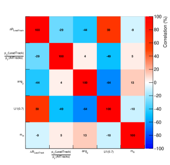
(b)

Figure 14: Correlation matrix 14(a) from the data and 14(b) from the cGAN.

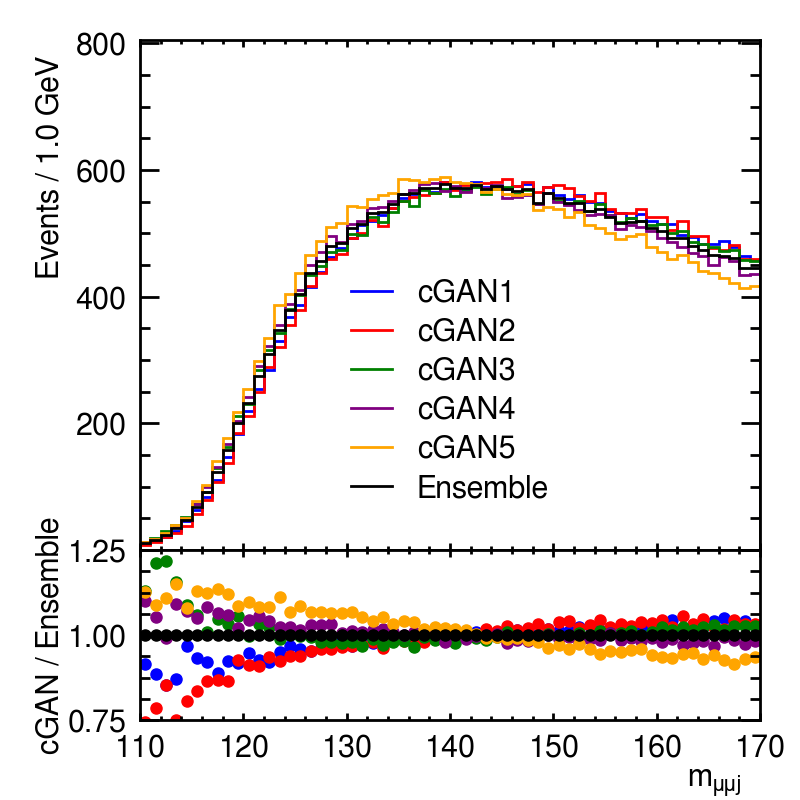
(a)

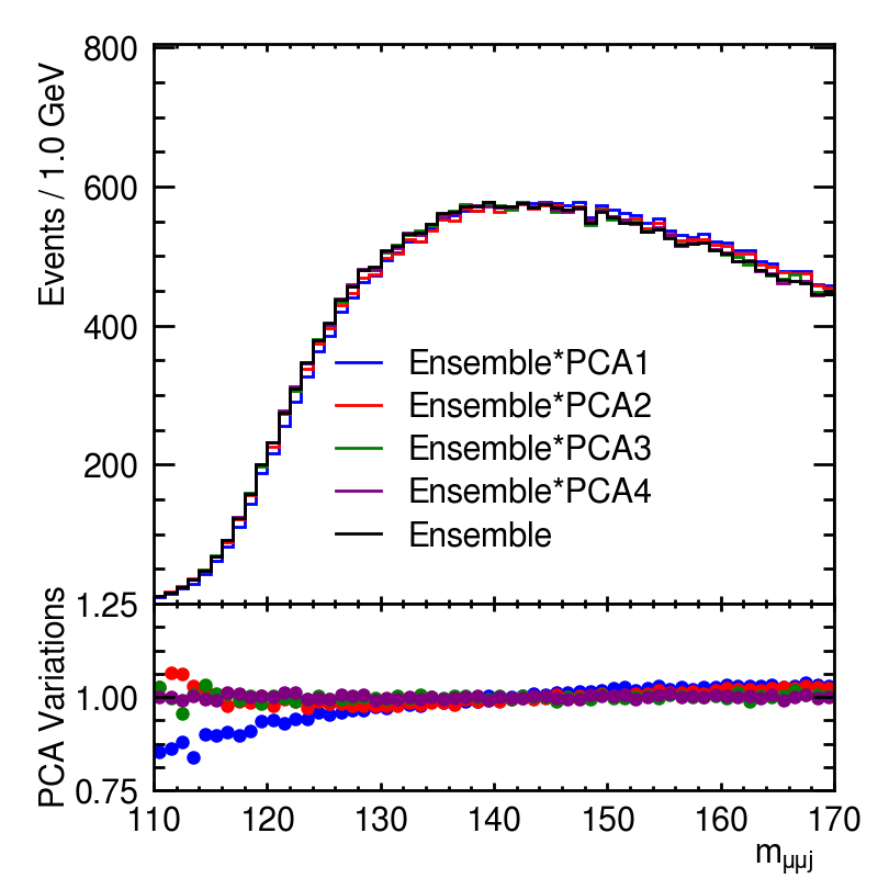
(b)

Figure 15: 15(a) Variation of the top five cGANs about their ensemble, and 15(b) the variations that correspond to $1\sigma$ uncertainties resulting from the principle component analysis.

Parameter	Value	Uncertainty ($\pm 1\sigma$)
$\mu_{\text{signal}}$	$-0.003$	$\pm 0.010$
$\mu_{\text{bkgd}}$	$1.001$	$\pm 0.008$
Shape uncertainty 1	$-0.36$	$\pm 0.27$
Shape uncertainty 2	$-0.31$	$\pm 0.52$

Table 5: Post-fit parameter values and their associated uncertainties.

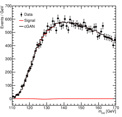
Figure 16: Post-fit $m_{\mu\mu\text{j}}$ distributions for a fit to the background-only dataset. The error bars on the markers represent the statistical uncertainty on the mock data. The sum of the signal and background models (upper red curve) and the signal model alone (lower red curve) are also shown.

3.6 Ensemble test using synthetic datasets

To further investigate the performance of the cGAN background modelling strategy, ensemble tests are performed using synthetic datasets. The results presented use 100 synthetic datasets, each consisting of $1.5\times 10^{6}$ background events generated to follow the function $1+x_{\text{c}}+2x_{\text{s}}+2x_{\text{c}}^{2}+x_{\text{s}}^{2}+x_{\text{c}}x_{\text{s}}$, and $0.5\times 10^{6}$ signal events generated from a Gaussian PDF in $x_{\text{c}}$ with mean 0.5 and standard deviation 0.025, with $x_{\text{c}}$ and $x_{\text{s}}$ in the range $[0,1]$. The conditioning variable is $x_{\text{c}}$ and the region $0.45<x_{\text{c}}<0.55$ is blinded in the training of the cGANs. The selection $x_{\text{s}}>0.95$ is applied, and this requirement is relaxed in the training of the cGANs. The average number of events in the $x_{\text{c}}$ blinding region that pass the $x_{\text{s}}$ selection is 11000, which is about 1.9 times higher than the analogous number for the validation study described in section 3.3, and if this were used in a single-bin counting experiment these events would have a statistical uncertainty of about 1%. Due to these very large synthetic datasets, this study is a highly stringent test of the robustness of the background model.

For each synthetic dataset, 100 cGANs are trained using $1\times 10^{6}$ background events, minus the events that are blinded in the training. The cGAN training procedure, architecture and hyperparameter optimisation procedure largely resemble that of the cGANs described in section 3.3. In particular, the same set of hyperparameters is optimised using a random scan over 100 sets of values, while the architecture and other hyperparameters are the same. An ensemble is built from the five most performant cGANs as determined with a similar $\chi^{2}$-based performance metric, defined using the remaining $0.5\times 10^{6}$ background events. The main exceptions to this are that the number of output (input) nodes of the generator (discriminator) network differ, the limits of the scan range of the number of training steps used were lowered, and due to the associated computational cost these cGANs were not trained until their performance approximately saturated.

Background shape uncertainties are estimated using a method similar to that described in section 3.4. An extended, binned, profile maximum likelihood fit to the $x_{\text{c}}$ distribution of events passing the $x_{\text{s}}$ selection is performed for each synthetic dataset, using the leading two background shape uncertainties. The pre-fit normalisation of the cGAN-based background estimate is set equal to the average number of synthetic data events passing the $x_{\text{s}}$ selection. Figure 17 shows the post-fit $x_{\text{c}}$ distributions for a fit to the background-only events passing the $x_{\text{s}}$ selection from one of the synthetic datasets. This exemplifies the large number of events generated that pass the $x_{\text{s}}$ selection for these synthetic datasets, and therefore the sensitivity with which this study tests this method.

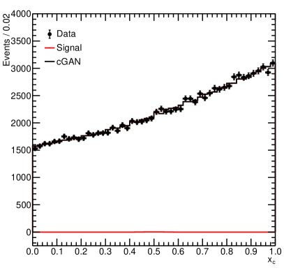
Figure 17: Post-fit $x_{\text{c}}$ distributions for a fit to the background-only dataset of one of the ensemble tests. The error bars on the markers represent the statistical uncertainty on the mock data. The sum of the signal and background models (upper red curve) and the signal model alone (lower red curve) are also shown.

The distribution of the signal (background) normalisations extracted from the fits (minus 1), normalised to their post-fit uncertainties, are shown in figure 18(a) (figure 18(b)). The distributions of the post-fit values of the nuisance parameters associated with the leading (sub-leading) background shape uncertainties are shown in figure 18(c) (figure 18(d)). It is observed that the data are able to constrain the shape nuisance parameters in the fit. The mean of the distribution of the post-fit signal normalisations, normalised to their post-fit uncertainties, is -0.38. Given the standard deviation of approximately unity for this pull variable, the mean of 100 of these quantities should have an uncertainty of about 0.1. Thus, for this implementation of the cGAN method, a small downward bias in the resulting estimates is observed. This bias may originate from limitations in the training of the cGANs. Such limitations include: the scan range of the number of training steps used was very likely lower than optimal; and dedicated reoptimisations of the architecture and many of the hyperparameters were not performed. As discussed in section 3.4, another contribution to this could originate from the interpolation in $x_{\text{c}}$.

An uncertainty with a magnitude of 38% times the post-fit signal normalisation uncertainty could be assigned to the signal normalisation to account for this bias, which would result in around a 7% increase to the total uncertainty. Additionally, the increase in the average post-fit signal normalisation uncertainty due to the shape uncertainties is 4%. As such, this method is providing a background estimate with a bias and a systematic uncertainty far below the statistical uncertainty of the signal normalisation, despite the large dataset in this search. The observed signal bias corresponds to only 0.4% of the average number of background events in the signal region that pass the $x_{\text{s}}$ selection, which is very small with respect to the typical MC-based modelling uncertainties. Furthermore, if the bias is due to limitations in the training of the cGANs, it is likely possible to improve the performance of this method.

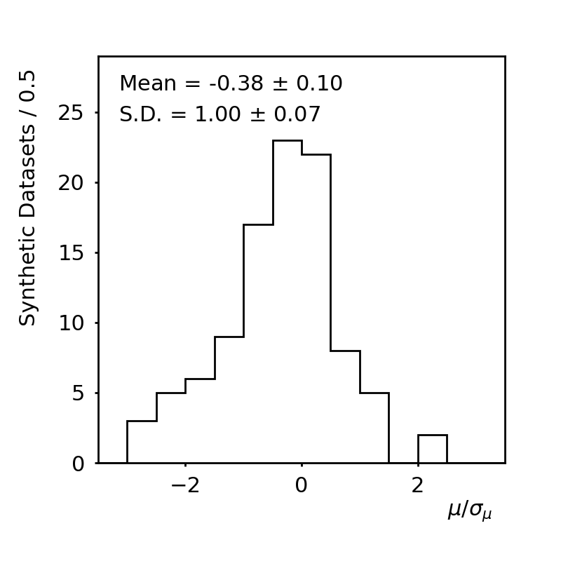
(a)

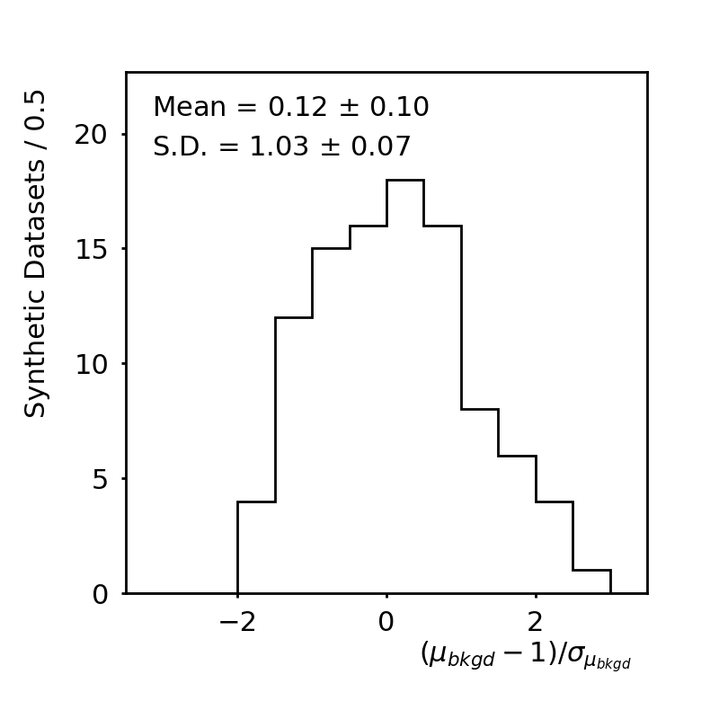
(b)

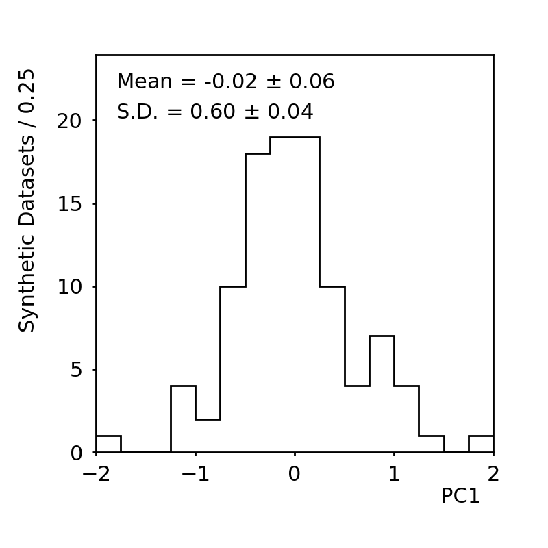
(c)

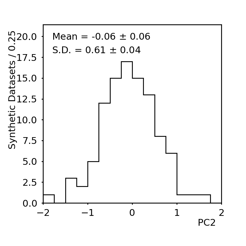
(d)

Figure 18: The pull distribution for 18(a) the signal strength and 18(b) the background normalisation. Furthermore, the post-fit values of the nuisance parameters associated with 18(c) the leading and 18(d) the sub-leading background shape uncertainties, are also presented. These results are extracted from fits to the synthetic datasets described in section 3.6.

4 Summary

A novel and widely applicable non-parametric data-driven background modelling method was presented, addressing typical shortcomings of often employed strategies, such as direct simulation and parametric models. Two techniques were discussed for its realisation. The first implementation uses data from a relaxed event selection to estimate a graph of conditional probability density functions of the variables used in the analysis. In the process the significant correlations between the variables are accounted for. A set of “pseudo-candidates” is then generated through ancestral sampling from this graph, which is subsequently propagated through the event selection. In the second technique, a generative adversarial network is trained to estimate the joint probability density function of the variables used in the analysis. As the training is performed on a relaxed event selection which excludes the signal region, the network is conditioned on the chosen blinding variable. Afterwards, the conditional probability density function is interpolated into the signal region to model the background. The application of the two methods on two benchmark analyses was presented in detail, including their implementation in terms of statistical inference and the derivation of associated systematic uncertainties. The performance in ensemble tests was also discussed. As demonstrated, the methods lend themselves to a wide spectrum of analyses, including in cases were other often employed methods are not applicable.

- (1) ATLAS collaboration, Observation of a new particle in the search for the Standard Model Higgs boson with the ATLAS detector at the LHC, Phys. Lett. B 716 (2012) 1 [1207.7214].
- (2) ATLAS collaboration, A search for the dimuon decay of the Standard Model Higgs boson with the ATLAS detector, Phys. Lett. B 812 (2021) 135980 [2007.07830].
- (3) P. Dauncey, M. Kenzie, N. Wardle and G. Davies, Handling uncertainties in background shapes: the discrete profiling method, JINST 10 (2015) P04015 [1408.6865].
- (4) CMS collaboration, A measurement of the Higgs boson mass in the diphoton decay channel, Phys. Lett. B 805 (2020) 135425 [2002.06398].
- (5) CMS collaboration, Evidence for Higgs boson decay to a pair of muons, JHEP 01 (2021) 148 [2009.04363].
- (6) M. Frate, K. Cranmer, S. Kalia, A. Vandenberg-Rodes and D. Whiteson, Modeling Smooth Backgrounds and Generic Localized Signals with Gaussian Processes, 1709.05681.
- (7) ATLAS collaboration, Search for exclusive Higgs and boson decays to and with the ATLAS detector, JHEP 07 (2018) 127 [1712.02758].
- (8) ATLAS collaboration, Searches for exclusive Higgs and boson decays into , , and at TeV with the ATLAS detector, Phys. Lett. B 786 (2018) 134 [1807.00802].
- (9) ATLAS collaboration, Search for Higgs and Boson Decays to with the ATLAS Detector, Phys. Rev. Lett. 117 (2016) 111802 [1607.03400].
- (10) ATLAS collaboration, Search for Higgs and Z Boson Decays to J/ and (nS) with the ATLAS Detector, Phys. Rev. Lett. 114 (2015) 121801 [1501.03276].
- (11) ATLAS collaboration, Search for Higgs Boson Decays into a Boson and a Light Hadronically Decaying Resonance Using 13 TeV Collision Data from the ATLAS Detector, Phys. Rev. Lett. 125 (2020) 221802 [2004.01678].
- (12) J. de Favereau, C. Delaere, P. Demin, A. Giammanco, V. Lemaître, A. Mertens et al., DELPHES 3, A modular framework for fast simulation of a generic collider experiment, JHEP 02 (2014) 057 [1307.6346].
- (13) CMS collaboration, Description and performance of track and primary-vertex reconstruction with the CMS tracker, JINST 9 (2014) P10009 [1405.6569].
- (14) A. Mathad, D. O’Hanlon, A. Poluektov and R. Rabadan, Efficient description of experimental effects in amplitude analyses, JINST 16 (2021) P06016 [1902.01452].
- (15) B. Nachman and D. Shih, Anomaly Detection with Density Estimation, Phys. Rev. D 101 (2020) 075042 [2001.04990].
- (16) A. Andreassen, B. Nachman and D. Shih, Simulation Assisted Likelihood-free Anomaly Detection, Phys. Rev. D 101 (2020) 095004 [2001.05001].
- (17) A. Andreassen and B. Nachman, Neural Networks for Full Phase-space Reweighting and Parameter Tuning, Phys. Rev. D 101 (2020) 091901 [1907.08209].
- (18) I. Goodfellow, Y. Bengio and A. Courville, Deep Learning. MIT Press, 2016.
- (19) T. Sjöstrand et al., An introduction to PYTHIA 8.2, Comput. Phys. Commun. 191 (2015) 159 [1410.3012].
- (20) S. Dulat et al., New parton distribution functions from a global analysis of quantum chromodynamics, Phys. Rev. D 93 (2016) 033006 [1506.07443].
- (21) T. Gleisberg, S. Hoeche, F. Krauss, M. Schonherr, S. Schumann, F. Siegert et al., Event generation with SHERPA 1.1, JHEP 02 (2009) 007 [0811.4622].
- (22) NNPDF collaboration, Parton distributions for the LHC Run II, JHEP 04 (2015) 040 [1410.8849].
- (23) M. Baak, S. Gadatsch, R. Harrington and W. Verkerke, Interpolation between multi-dimensional histograms using a new non-linear moment morphing method, Nucl. Instrum. Meth. A 771 (2015) 39 [1410.7388].
- (24) I. J. Goodfellow et al., Generative Adversarial Networks, 1406.2661.
- (25) A. Radford, L. Metz and S. Chintala, Unsupervised representation learning with deep convolutional generative adversarial networks, 1511.06434.
- (26) T. Karras, T. Aila, S. Laine and J. Lehtinen, Progressive growing of gans for improved quality, stability, and variation, 1710.10196.
- (27) A. Brock, J. Donahue and K. Simonyan, Large scale gan training for high fidelity natural image synthesis, 1809.11096.
- (28) H. Zhang, T. Xu, H. Li, S. Zhang, X. Wang, X. Huang et al., Stackgan: Text to photo-realistic image synthesis with stacked generative adversarial networks, in Proceedings of the IEEE international conference on computer vision, pp. 5907–5915, 2017, 1612.03242.
- (29) L. Wang, W. Chen, W. Yang, F. Bi and F. R. Yu, A state-of-the-art review on image synthesis with generative adversarial networks, IEEE Access 8 (2020) 63514.
- (30) X. Yi, E. Walia and P. Babyn, Generative adversarial network in medical imaging: A review, Medical Image Analysis 58 (2019) 101552.
- (31) Y. Alanazi, N. Sato, P. Ambrozewicz, A. N. H. Blin, W. Melnitchouk, M. Battaglieri et al., A survey of machine learning-based physics event generation, 2106.00643.
- (32) A. Butter and T. Plehn, Generative Networks for LHC events, 2008.08558.
- (33) A. Butter, S. Diefenbacher, G. Kasieczka, B. Nachman and T. Plehn, GANplifying event samples, SciPost Phys. 10 (2021) 139 [2008.06545].
- (34) A. Radovic, M. Williams, D. Rousseau, M. Kagan, D. Bonacorsi, A. Himmel et al., Machine learning at the energy and intensity frontiers of particle physics, Nature 560 (2018) 41.
- (35) D. Guest, K. Cranmer and D. Whiteson, Deep Learning and its Application to LHC Physics, Ann. Rev. Nucl. Part. Sci. 68 (2018) 161 [1806.11484].
- (36) D. Bourilkov, Machine and Deep Learning Applications in Particle Physics, Int. J. Mod. Phys. A 34 (2020) 1930019 [1912.08245].
- (37) M. D. Schwartz, Modern Machine Learning and Particle Physics, 2103.12226.
- (38) G. Karagiorgi, G. Kasieczka, S. Kravitz, B. Nachman and D. Shih, Machine Learning in the Search for New Fundamental Physics, 2112.03769.
- (39) M. Feickert and B. Nachman, A Living Review of Machine Learning for Particle Physics, 2102.02770.
- (40) S. Otten et al., Event Generation and Statistical Sampling for Physics with Deep Generative Models and a Density Information Buffer, 1901.00875.
- (41) A. Butter, T. Plehn and R. Winterhalder, How to GAN LHC Events, SciPost Phys. 7 (2019) 075 [1907.03764].
- (42) SHiP collaboration, Fast simulation of muons produced at the SHiP experiment using Generative Adversarial Networks, JINST 14 (2019) P11028 [1909.04451].
- (43) J. Arjona Martínez et al., Particle Generative Adversarial Networks for full-event simulation at the LHC and their application to pileup description, in 19th International Workshop on Advanced Computing and Analysis Techniques in Physics Research: Empowering the revolution: Bringing Machine Learning to High Performance Computing, 12, 2019, 1912.02748.
- (44) ATLAS collaboration, Deep generative models for fast shower simulation in ATLAS, J. Phys. Conf. Ser. 1525 (2020) 012077.
- (45) B. Hashemi et al., LHC analysis-specific datasets with Generative Adversarial Networks, 1901.05282.
- (46) R. Di Sipio, M. Faucci Giannelli, S. Ketabchi Haghighat and S. Palazzo, DijetGAN: A Generative-Adversarial Network Approach for the Simulation of QCD Dijet Events at the LHC, JHEP 08 (2019) 110 [1903.02433].
- (47) R. Di Sipio, M. Faucci Giannelli, S. Ketabchi Haghighat and S. Palazzo, A Generative-Adversarial Network Approach for the Simulation of QCD Dijet Events at the LHC, PoS LeptonPhoton2019 (2019) 050.
- (48) S. Farrell et al., Next Generation Generative Neural Networks for HEP, EPJ Web Conf. 214 (2019) 09005.
- (49) Y. Alanazi et al., Simulation of electron-proton scattering events by a Feature-Augmented and Transformed Generative Adversarial Network (FAT-GAN), 2001.11103.
- (50) S. Vallecorsa, F. Carminati and G. Khattak, 3D convolutional GAN for fast simulation, EPJ Web Conf. 214 (2019) 02010.
- (51) M. Mirza and S. Osindero, Conditional Generative Adversarial Nets, 1411.1784.
- (52) A. Hallin, J. Isaacson, G. Kasieczka, C. Krause, B. Nachman, T. Quadfasel et al., Classifying Anomalies THrough Outer Density Estimation (CATHODE), 2109.00546.
- (53) G. Papamakarios, T. Pavlakou and I. Murray, Masked autoregressive flow for density estimation, Advances in neural information processing systems 30 (2017) [1705.07057].
- (54) D. Curtin et al., Exotic decays of the 125 GeV Higgs boson, Phys. Rev. D 90 (2014) 075004 [1312.4992].
- (55) CDF collaboration, A Measurement of and in collisions at GeV, Phys. Rev. D 44 (1991) 29.
- (56) M. Cacciari, G. P. Salam and G. Soyez, The anti- jet clustering algorithm, JHEP 04 (2008) 063 [0802.1189].
- (57) M. Cacciari, G. P. Salam and G. Soyez, FastJet User Manual, Eur. Phys. J. C 72 (2012) 1896 [1111.6097].
- (58) L. G. Almeida, S. J. Lee, G. Perez, G. F. Sterman, I. Sung and J. Virzi, Substructure of high- Jets at the LHC, Phys. Rev. D 79 (2009) 074017 [0807.0234].
- (59) I. Moult, L. Necib and J. Thaler, New Angles on Energy Correlation Functions, JHEP 12 (2016) 153 [1609.07483].
- (60) F. Chollet et al., “Keras.” https://keras.io, 2015.
- (61) M. Abadi, A. Agarwal, P. Barham, E. Brevdo, Z. Chen, C. Citro et al., TensorFlow: Large-scale machine learning on heterogeneous systems, 2015.
- (62) LHC Higgs Cross Section Working Group collaboration, Handbook of LHC Higgs Cross Sections: 4. Deciphering the Nature of the Higgs Sector, 1610.07922.