Reliability Assessment and Safety Arguments for Machine Learning Components in System Assurance

Abstract.

The increasing use of Machine Learning (ML) components embedded in autonomous systems—so-called Learning-Enabled Systems (LESs)—has resulted in the pressing need to assure their functional safety. As for traditional functional safety, the emerging consensus within both, industry and academia, is to use assurance cases for this purpose. Typically assurance cases support claims of reliability in support of safety, and can be viewed as a structured way of organising arguments and evidence generated from safety analysis and reliability modelling activities. While such assurance activities are traditionally guided by consensus-based standards developed from vast engineering experience, LESs pose new challenges in safety-critical application due to the characteristics and design of ML models. In this article, we first present an overall assurance framework for LESs with an emphasis on quantitative aspects, e.g., breaking down system-level safety targets to component-level requirements and supporting claims stated in reliability metrics. We then introduce a novel model-agnostic Reliability Assessment Model (RAM) for ML classifiers that utilises the operational profile and robustness verification evidence. We discuss the model assumptions and the inherent challenges of assessing ML reliability uncovered by our RAM and propose solutions to practical use. Probabilistic safety argument templates at the lower ML component-level are also developed based on the RAM. Finally, to evaluate and demonstrate our methods, we not only conduct experiments on synthetic/benchmark datasets but also scope our methods with case studies on simulated Autonomous Underwater Vehicles and physical Unmanned Ground Vehicles.

20cm(1cm,1cm) Accepted by ACM Transactions on Embedded Computing Systems https://dl.acm.org/journal/tecs

LIST OF ACRONYMS
	ACU	Average Cell Unastuteness	MEM	Minimum Endogenous Mortality
	AE	Adversarial Example	ML	Machine Learning
	ALARP	As Low As Reasonably Practicable	MLE	Maximum Likelihood Estimation
	AUV	Autonomous Underwater Vehicles	OP	Operational Profile
	CAE	Claims Arguments Evidence	PDF	Probability Density Function
	CLT	Central Limiting Theorem	PID	Proportional-Integral-Derivative
	DL	Deep Learning	$pmi$	probability of misclassification per random input
	DVL	Doppler Velocity Log	RAM	Reliability Assessment Models
	FTA	Fault-Tree Analysis	RAS	Robotics and Autonomous Systems
	GALE	Globally At Least Equivalent	ROS	Robot Operating System
	GSN	Goal Structuring Notation	SE	Substantially Equivalent
	HAZOP	Hazard and Operability Study	SMC	Simple Monte Carlo
	IMU	Inertial Measurement Unit	UGV	Unmanned Ground Vehicle
	KDE	Kernel Density Estimation	V&V	Verification and Validation
	LES	Learning-Enabled Systems	VAE	Variational Auto-Encoders

1. Introduction

Industry is increasingly adopting AI/Machine Learning (ML) algorithms to enhance the operational performance, dependability, and lifespan of products and service – systems with embedded ML-based software components. For such Learning-Enabled Systems (LES), in safety-related applications high reliability is essential to ensure successful operations and regulatory compliance. For instance, several fatalities were caused by the failures of LES built in Uber and Tesla’s cars. IBM’s Watson, the decision-making engine behind the Jeopardy AI success, has been deemed a costly and potentially deadly failure when extended to medical applications like cancer diagnosis. Key industrial foresight reviews have identified that the biggest obstacle to reap the benefits of ML-powered Robotics and Autonomous Systems (RAS) is the assurance and regulation of their safety and reliability (Lane et al., 2016). Thus, there is an urgent need to develop methods that enable the dependable use of AI/ML in critical applications and, just as importantly, to assess and demonstrate the dependability for certification and regulation.

For traditional systems, safety regulation is guided by well-established standards/policies, and supported by mature development processes and Verification and Validation (V&V) techniques. The situation is different for LES: they are disruptively novel and often treated as a black box with the lack of validated standards/policies (Bloomfield et al., 2019), while they require new and advanced analysis for the complex requirements in their safe and reliable function. Such analysis needs to be tailored to fully evaluate the new character of ML (Alves et al., 2018; Burton et al., 2020; Koopman et al., 2019), despite some progress made recently (Huang et al., 2020). This reinforces the need for not only an overall methodology/framework in assuring the whole LES, but also innovations in safety analysis and reliability modelling for ML components, which motivate our work.

In this article, we first propose an overall assurance framework for LES, presented in Claims-Arguments-Evidence (CAE) assurance cases (Bloomfield and Bishop, 2010). While inspired by (Bloomfield et al., 2021), ours is with greater emphasis on arguing for quantitative safety requirements. This is because the unique characteristics of ML increase apparent non-determinism (Johnson, C. W., 2018) that explicitly requires probabilistic claims to capture the uncertainties in its assurance (Zhao et al., 2020a; Asaadi et al., 2020a; Bloomfield and Rushby, 2020). To demonstrate the overall assurance framework as an end-to-end methodology, we also consider important questions on how to derive and validate (quantitative) safety requirements and how to break them down to functionalities of ML components for a given LES. Indeed, there should not be any generic, definitive, or fixed answers to those hard questions for now, since AI/ML is an emerging technology that is still heavily in flux. That said, we propose a solution that we believe is the most practical for the moment: we exercise the method (Qi et al., 2022) which extends the Hazard and Operability Study (HAZOP) (a systematic hazards identification method) (Swann and Preston, 1995), quantitative Fault-Tree Analysis (FTA) (a common probabilistic root-cause analysis) (Lee et al., 1985), and propose to leverage existing regulation principles to validate the acceptable and tolerable safety risk, e.g., Globally At Least Equivalent (GALE) to non-AI/ML systems or human performance.

Upon establishing safety/reliability requirements on low-level functionalities of ML components, we build dedicated Reliability Assessment Models (RAM). In this article, we mainly focus on assessing the reliability of the classification function of the ML component, extending our initial RAM in (Zhao et al., 2021a) with more practical considerations for scalability. Our RAM explicitly takes the Operational Profile (OP) information and robustness evidence into account, because: (i) software reliability, as a user-centred property, depends on the end-users’ behaviours (Littlewood and Strigini, 2000), and the OP (quantifying how the software will be operated (Musa, 1993)) should therefore be explicitly modelled in the assessment; (ii) a RAM without considering robustness evidence is not convincing given ML is notorious to be unrobust. To the best of our knowledge, our RAM is the first to consider both, the OP and robustness evidence. It is inspired by partition-based testing (Hamlet and Taylor, 1990; Pietrantuono et al., 2020), operational/statistical testing (Strigini and Littlewood, 1997; Zhao et al., 2020c) and ML robustness evaluation (Webb et al., 2019). Our RAM is model-agnostic and designed for pre-trained ML models, yielding estimates of, e.g., expectation or confidence bounds on the metric probability of misclassification per random input (pmi). Then, we present a set of safety case templates to support reliability claims stated in pmi based on our new RAM—the “backbone” of the probabilistic safety arguments for ML components, where the key argument is over the rigour of the four main steps of the RAM.

Finally, we conduct comprehensive case studies based on Autonomous Underwater Vehicles (AUV) and Unmanned Ground Vehicle (UGV) in both simulated and physical environments to demonstrate and validate our methods. All source code, ML models, datasets and experimental results used in this work are publicly available at the our project repository https://github.com/Solitude-SAMR with video demos at https://youtu.be/akY8f5sSFpY and https://youtu.be/E95vh5sxs7I.

Summary of Contributions

The key contributions of this work include:

• An assurance case framework for LES that: (i) emphasises the arguments for quantitative claims on safety and reliability; (ii) with an “end-to-end” chain of safety analysis and reliability modelling methods for arguments ranging from the very top safety claim of the whole LES to low-level V&V evidence of ML components.

• A first RAM evaluating reliability for ML software, leveraging both the OP information and robustness evidence. Moreover, based on the RAM, templates of probabilistic arguments for reliability claims on ML software are developed.

• Identification of open challenges in building safety arguments for LES and highlighting the inherent difficulties of assessing ML reliability, uncovered by our overall assurance framework and the proposed RAM, respectively. Potential solutions are discussed and mapped onto on-going studies to advance in this research direction.

• A prototype tool of our RAM and a simulator platform of AUV for underwater missions. Besides, real-world case studies based on a physical UGV and a healthcare application are conducted to support the proposed approaches.

Organisation of this Article

The scope and related work are summarised in Section 2. After presenting preliminaries in Section 3, we outline our overall system-level assurance framework in Section 4. We focus on the ML-component level where the RAM is described in detail in Section 5. We then present case studies in Section 6. Furthermore, in-depth discussions are provided in Section 7. Finally, we conclude and outline plans for future work in Section 8.

2. Scope and Related Work

The aim of this work is to bridge the gap between local robustness evaluation evidence to system-level safety claims. By the interdisciplinary nature of the target problem, it spans across different subjects including ML, software engineering, safety assurance and reliability engineering. We refer to Fig. 1 to highlight the scope and position of this paper (covering blocks ④, ⑤, ⑨, ⑬) as what follows.

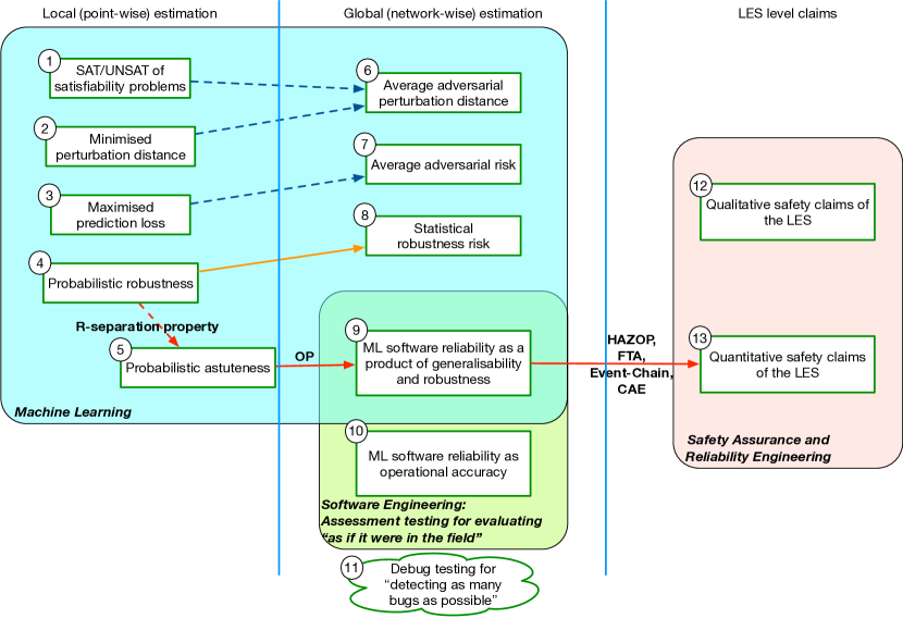
Figure 1. Scope and position: This paper presents a chain of methods in blocks ⑤, ⑨ and ⑬ across three levels linked by techniques shown on the red edges, which has its roots in the probabilistic notion of local robustness (block ④). In stark contrast, other blocks at the local (i.e., point-wise robustness) level concern binary and extreme-cases that are non-probabilistic. Consequently, at the global network-wide level (i.e., the ML software), successor blocks of those non-probabilistic metrics can only consider averaged worst-case robustness (blocks ⑥ and ⑦). At this ML software level, our RAM (block ⑨) agrees with the statistical robustness (block ⑧) that describes the pervasiveness of AEs in the input space, but with extra considerations on the oracle and OP and thus unifies robustness (astuteness, to be exact) and generalisability. Blocks ⑨+⑩ and ⑪ are representing two distinct types of testing in software engineering, i.e. assessment testing vs debug testing, while our RAM falls into the former category making the latter category irrelevant. Unlike ours (Block ⑨), existing assessment testing methods only consider the OP and ignores the point-wise robustness evidence (Block ⑩). Finally, at the the whole system level of LES, our work supports quantitative safety claims.

2.1. ML Robustness Evaluation

Despite the exact definitions of robustness vary in literatures, they all share the intuition that inputs in a small region (usually a norm ball defined in some $L_{p}$-norm distance) have the same prediction label. Inside the local region, if an input is classified differently to the central point by the ML model, then it is detected as an Adversarial Example (AE). In recent years, great efforts have been made to study the local robustness of ML models, while they formalise the problem in various ways and propose different evaluation metrics accordingly.

As shown in the first column of Fig. 1, the most classical type of approaches is by framing the robustness evaluation as a satisfiability problem that usually can be solved by SAT/SMT solvers (Huang et al., 2017; Katz et al., 2017; Gehr et al., 2018; Singh et al., 2019). Thus, given a local perturbation distance as constraints, a binary metric (i.e., Sat/Unsat) can be evaluated (block ①). The main limitation of such methods is their scalability to the size of ML models and input dimensions. A more scalable type of methods is based on adversarial attacks, which normally requires an expensive gradient computation to detect AE s and compute a minimised perturbation distance (block ②), e.g., (Moosavi-Dezfooli et al., 2016, 2017; Aminifar, 2020; Weng et al., 2019). Similarly, (Weng et al., 2018) converts robustness analysis into a local Lipschitz constant estimation problem, deriving a lower bound on the minimal perturbation distance required to craft an AE. When considering adversarial training, maximised prediction loss (block ③) is often the metric of interest, e.g., (Madry et al., 2018) introduces the adversarial risk which is the maximum prediction loss within norm balls to measure the local robustness. They further apply this metric as the training loss to train ML modela that are more resistant to adversarial attacks.

At the local level, all aforementioned methods essentially answer the binary question of whether there exist any AE s in some perturbation distance. As argued by (Webb et al., 2019), they all suffer from two major drawbacks: i) they provide no notion of how robust the model is whenever an AE can be found; ii) there is a computational problem whenever no or only rare AE s exist. To address the shortfalls, (Webb et al., 2019) develops a new measure of probabilistic robustness (block ④) under a local distribution over a set of inputs. Arguably, such probabilistic metric is of more practical interest in twofold (Webb et al., 2019): i) binary verification concerning extreme cases is neither necessary nor realistically achievable, i.e., one actually desires to know the proportion of AEs in the input set, not just a binary answer as to whether it is robust or not; ii) all practical applications have acceptable level of risk, so that instead of confirming that this probability is exactly zero, showing the probability of a violation below a required threshold is good enough. We concur with these key insights and extend the probabilistic robustness to probabilistic astuteness (block ⑤) in this work, by casting constraints (i.e., the $r$-separation property in Remark 3) on the norm ball radius as a principled way of determine the oracle (cf. later Remark 2). More explicitly, in Table 5 of Appendix C, we highlight the new characteristics of our block ⑤ by comparing with DeepFool (Moosavi-Dezfooli et al., 2016) and AI2 (Gehr et al., 2018) locally, showing the differences between their inputs and outputs.

We usually concern the overall robustness of the ML model (Wang et al., 2021), i.e., its robustness across the range of possible inputs that the ML component will see in the real operation (Kurakin et al., 2018; Zhao et al., 2021b). This has motivated “global” or “network-wide” robustness metrics (second column in Fig. 1). Stemming from the corresponding local robustness metrics, the common metrics at this level simply take the average over a set of local robustness evaluation from regions represented by the training dataset, e.g., average minimal adversarial distance (Fawzi et al., 2018), average adversarial risk (Madry et al., 2018) (blocks ⑥ and block ⑦ respectively). As discussed by (Wang et al., 2021), it is often misleading to use those metrics with binary extreme-case meanings at network-wide level—indeed, an ML model can only be perfectly worst-case robust if it is robust to all possible perturbations of all inputs, something which will very rarely be achievable in practice. Later in our experiments, we highlight the characteristics of our new block ⑨ compared to block ⑥ (that uses DeepFool (Moosavi-Dezfooli et al., 2016) locally) in Table 6 of Appendix C. We may observe they are different metrics by nature, while arguably ours is of more practical interest. To overcome the problem, (Wang et al., 2021) proposes a set of statistical robustness risks (block ⑧) which assess the overall probabilistic robustness by averaging the point-wise statistical robustness of (Webb et al., 2019). Aligning with the same idea, we build upon our local probabilistic astuteness metric to get the reliability of the ML component (block ⑨). Unlike (Wang et al., 2021), we explicitly incorporate the OP and oracle information.

2.2. OP-based Software Reliability Assessment

OP-based software testing, also known as statistical/operational testing (Strigini and Littlewood, 1997), is an established practice and supported by industry standards for conventional systems. There is a huge body of literature in the traditional software reliability community on OP-based testing and reliability modelling techniques, e.g., (Bertolino et al., 2021; Bishop and Povyakalo, 2017; Pietrantuono et al., 2020; Zhao et al., 2020c). In contrast to this, OP-based software testing for ML components is still in its infancy: to the best of our knowledge, there are only two recent works that explicitly consider the OP in testing. Li et al. (Li et al., 2019) propose novel stratified sampling based on ML specific information to improve the testing efficiency. Similarly, Guerriero et al. (Guerriero et al., 2021) develop a test case sampling method that leverages “auxiliary information for misclassification” and provides unbiased testing accuracy estimators. The motivation behind these two works is to leverage advanced sampling techniques to reduce the cost of testing in the operational dataset to yield the operational accuracy (block ⑩), However, neither of them considers robustness evidence in their assessment like our RAM does.

At the whole LES level, there are reliability studies based on operational and statistical data, e.g., (Kalra and Paddock, 2016; Zhao et al., 2019b) for self-driving cars, (Hereau et al., 2020; Zhao et al., 2019a) for AUV, and (Robert et al., 2020) for agriculture robots doing autonomous weeding. However, knowledge from low-level ML components is usually ignored. In (Zhao et al., 2020c), we improved (Kalra and Paddock, 2016) by providing a Bayesian mechanism to combine such knowledge, but did not discuss where to obtain the knowledge. In that sense, this article also contains follow-up work of (Zhao et al., 2020c), providing the prior knowledge required based on the OP and robustness evidence.

Given that the OP is essentially a distribution defined over the whole input space, a related topic is the distribution-aware testing for Deep Learning (DL) (block ⑪) developed recently. For instance, in (Berend, 2021), distribution-guided coverage criteria are developed to guide the generation of new unseen test cases while identifying the validity of errors in DL system tasks. In (Dola et al., 2021), a generative model is utilised to guide the generation of valid test cases. However, all existing distribution-aware testing methods are designed for detecting as many AEs as possible, instead of trying to do reliability assessment like ours, which are two distinct types of testing (Frankl et al., 1998; Bertolino et al., 2017; Cotroneo et al., 2016).

2.3. Assurance Cases for AI/ML-powered Autonomous Systems

Work on safety arguments and assurance cases for AI/ML models and autonomous systems has emerged in recent years. Burton et al. (Burton et al., 2020) draw a broad picture of assuring AI and identify/categorise the “gap” that arises across the development process. Alves et al. (Alves et al., 2018) present a comprehensive discussion on the aspects that need to be considered when developing a safety case for increasingly autonomous systems that contain ML components. Similarly, in (Bloomfield et al., 2019), an initial safety case framework is proposed with discussions on specific challenges for ML, which is later implemented with more details in (Bloomfield et al., 2021). A recent work (Javed et al., 2021) also explicitly suggests the combination of HAZOP and FTA in safety cases for identifying/mitigating hazards and deriving safety requirements (and safety contracts) when studying Industry 4.0 systems. In (Koopman et al., 2019), safety arguments that are being widely used for conventional systems—including conformance to standards, proven in use, field testing, simulation, and formal proofs—are recapped for autonomous systems with discussions on the potential pitfalls. Both, (Matsuno et al., 2019) and (Ishikawa and Matsuno, 2018), propose utilising continuously updated arguments to monitor the weak points and the effectiveness of their countermeasures, while a similar mechanism is also suggested in our assurance case, e.g., continuously monitor/estimate key parameters of our RAM—all essentially aligns with the idea of dynamic assurance cases (Calinescu et al., 2018; Asaadi et al., 2020b).

Although the aforementioned works have inspired this article, our assurance framework is with greater emphasis on, and thus complements them from, the quantitative aspects (block ⑬), e.g., reasoning for reliability claims stated in bespoke measures and breaking down system-level safety targets to component-level quantitative requirements. Also exploring quantitative assurance, Asaadi et al. (Asaadi et al., 2020a) identifies dedicated assurance measures that are tailored for properties of aviation systems.

3. Preliminaries

3.1. Assurance Cases, CAE Notations and CAE Blocks

Assurance cases are developed to support claims in areas such as safety, reliability and security. They are often called by more specific names like security cases (Knight, 2015) and safety cases (Bishop and Bloomfield, 2000). A safety case is a compelling, comprehensive, defensible, and valid justification of the system safety for a given application in a defined operating environment; it is therefore a means to provide the grounds for confidence and to assist decision making in certification (Bloomfield and Bishop, 2010). For decades, safety cases have been widely used in the European safety community to assure system safety. Moreover, they are mandatory in the regulation for systems used in safety-critical industries in some countries, e.g., in the UK for nuclear energy (UK Office for Nuclear Regulation, 2019). Early research in safety cases has mainly focused on their formulation in terms of claims, arguments, and evidence elements based on fundamental argumentation theories like the Toulmin model (S. Toulmin, 1958). The two most popular notations are CAE (Bloomfield and Bishop, 2010) and Goal Structuring Notation (GSN) (Kelly, 1999). In this article, we choose the former to present our assurance case templates.

A summary of the CAE notations is provided in Fig. 2. The CAE safety case starts with a top claim, which is then supported through an argument by sub-claims. Sub-claims can be further decomposed until being supported by evidence. A claim may be subject to some context, represented by general purpose other nodes, while assumptions (or warranties) of arguments that need to be explicitly justified form new side-claims. A sub-case repeats a claim presented in another argument module. Notably, the basic concepts of CAE are supported by safety standards like ISO/IEC15026-2. Readers are referred to (Bloomfield and Rushby, 2020; Bloomfield et al., 2021) for more details on all CAE elements.

The CAE framework additionally consists of CAE blocks that provide five common argument fragments and a mechanism for separating inductive and deductive aspects of the argumentation. These were identified by empirical analysis of real-world safety cases (Bloomfield and Netkachova, 2014). The five CAE blocks representing the restrictive set of arguments are:

• Decomposition: partition some aspect of the claim—“divide and conquer”.

• Substitution: transform a claim about an object into a claim about an equivalent object.

• Evidence Incorporation: evidence supports the claim, with emphasis on direct support.

• Concretion: some aspect of the claim is given a more precise definition.

• Calculation (or Proof): some value of the claim can be computed or proven.

An illustrative use of CAE blocks is shown in Fig. 2, while more detailed descriptions can be found in (Bloomfield and Netkachova, 2014; Bloomfield et al., 2021).

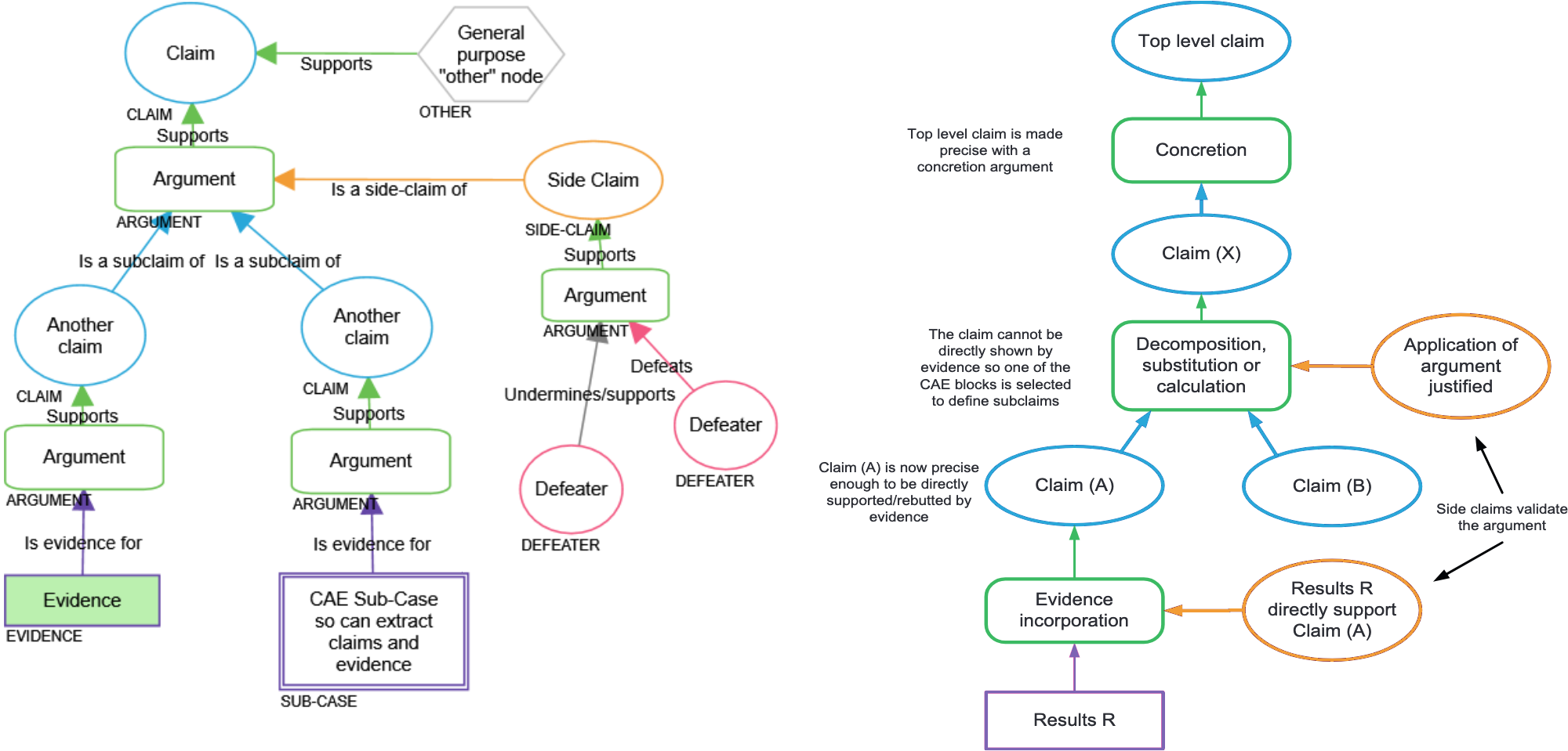
Figure 2. Summary of the CAE notations (lhs) and an example of CAE block use (rhs), cited from (Bloomfield et al., 2021).

3.2. HAZOP and FTA

HAZOP is a structured and systematic safety analysis technique for risk management, which is used to identify potential hazards for the system in the given operating environment. HAZOP is based on a theory that assumes risk events are caused by deviations from design or operating intentions. Identification of such deviations is facilitated by using sets of “guide words” (e.g., too much, too little and no) as a systematic list of deviation perspectives. It is commonly performed by a multidisciplinary team of experts during brainstorming sessions. HAZOP is a technique originally developed and used in chemical industries. There are studies that successfully apply it to software-based systems (Swann and Preston, 1995). Readers will see an illustrative example in later sections, while we refer to (Crawley and Tyler, 2015) for more details.

FTA is a quantitative safety analysis technique on how failures propagate through the system, i.e., how component failures lead to system failures. The fundamental concept in FTA is the distillation of system component faults that can lead to a top-level event into a structured diagram (fault tree) using logic gates (e.g., AND, OR, Exclusive-OR and Priority-AND). We show a concrete example of FTA in our case study section, while a full tutorial of developing FTA is out of the scope of this article, and readers are referred to (Ruijters and Stoelinga, 2015) for more details.

3.3. OP Based Software Reliability Assessment

The delivered reliability, as an user-centred and probabilistic property, requires to model the end-users’ behaviours (in the operating environments) and to be formally defined by a quantitative metric (Littlewood and Strigini, 2000). Without loss of generality, we focus on pmi as a generic metric for ML classifiers, where inputs can, e.g., be images acquired by a robot for object recognition.

Definition 0 (pmi).

We denote the unknown pmi by a variable $\lambda$, which is formally defined as

(1) $$\lambda:=\int_{x\in\mathcal{X}}I_{\{x\text{ causes a misclassification}\}}(x)\mathsf{Op}(x)\mathop{}\!\mathrm{d}{x}\ ,$$

where $x$ is an input in the input domain $\mathcal{X}$, and ${I}_{\tt S}(x)$ is an indicator function—it is equal to $1$ when S is true and equal to $0$ otherwise. The function $\mathsf{Op}(x)$ returns the probability that $x$ is the next random input.

Intuitively, if we randomly selected an input from the input domain according to the distribution of OP, the probability of the event that this input being misclassified is measured by pmi. In other words, a “frequentist” interpretation of pmi is that it is the limiting relative frequency of inputs for which the classifier fails in an infinite sequence of independently selected inputs. In this regard, pmi is a natural extension of the conventional reliability metric probability of failure on demand (pfd) (Zhao et al., 2017), but retrofitted for ML classifiers.

Remark 1 (OP).

The OP (Musa, 1993) is a notion used in software engineering to quantify how the software will be operated. Mathematically, the OP is a Probability Density Function (PDF) defined over the whole input domain $\mathcal{X}$.

We highlight this Remark 1, because we use probability density estimators to approximate the OP from the collected operational dataset in our RAM developed in Section 5.

By the definition of pmi, successive inputs are assumed to be independent. It is therefore common to use a Bernoulli process as the mathematical abstraction of the stochastic failure process, which implies a Binomial likelihood. For traditional software, upon establishing the likelihood, RAMs on estimating $\lambda$ vary case by case—from the basic Maximum Likelihood Estimation (MLE) to Bayesian estimators tailored for certain scenarios when, e.g., seeing no failures (Miller et al., 1992; Bishop et al., 2011), inferring ultra-high reliability (Zhao et al., 2020c), with certain forms of prior knowledge like perfectioness (Strigini and Povyakalo, 2013), with vague prior knowledge expressed in imprecise probabilities (Walter and Augustin, 2009; Zhao et al., 2019a), with uncertain OP s (Bishop and Povyakalo, 2017; Pietrantuono et al., 2020), etc.

OP based RAMs designed for traditional software fail to consider new characteristics of ML, e.g., the lack of robustness and a high dimensional input space. Specifically, it is quite hard to gather the required prior knowledge when taking into account the new ML characteristics in the aforementioned Bayesian RAMs. At the same time, frequentist RAMs would require a large sample size to gain enough confidence in the estimates due to the extremely large population size (e.g., the high dimensional pixel space for images).

3.4. ML Robustness and the $R$-Separation Property

ML is known not to be robust. Robustness requires that the decision of the ML model ${\mathcal{M}}$ is invariant against small perturbations on inputs. That is, all inputs in a region $\eta\subset\mathcal{X}$ have the same prediction label, where usually the region $\eta$ is a small norm ball (in an $L_{p}$-norm distance) of radius $\epsilon$ around an input $x$. Inside $\eta$, if an input $x^{\prime}$ is classified differently to $x$ by ${\mathcal{M}}$, then $x^{\prime}$ is an AE. Robustness can be defined either as a binary metric (if there exists any AE in $\eta$) or as a probabilistic metric (how likely the event of seeing an AE in $\eta$ is). The former aligns with formal verification, e.g. (Huang et al., 2017), while the latter is normally used in statistical approaches, e.g. (Webb et al., 2019). The former “verification approach” is the binary version of the latter “stochastic approach”.

Definition 0 (robustness).

Similar to (Webb et al., 2019), we adopt the more general probabilistic definition on the robustness of the model ${\mathcal{M}}$ (in a region $\eta$ and to a target label $y$):

(2) $$R_{{\mathcal{M}}}(\eta,y):=\int_{x\in\eta}I_{\{{\mathcal{M}}(x)\text{ predicts label }y\}}(x)\mathsf{Op}(x\mid x\in\eta)\mathop{}\!\mathrm{d}{x}\ ,$$

where $\mathsf{Op}(x\mid x\in\eta)$ is the conditional OP of region $\eta$ (precisely the “input model” used by both (Webb et al., 2019) and (Weng et al., 2019)).

We highlight the following two remarks regarding robustness:

Remark 2 (astuteness).

Reliability assessment only concerns the robustness to the ground truth label, rather than an arbitrary label $y$ in $R_{{\mathcal{M}}}(\eta,y)$. When $y$ is such a ground truth, robustness becomes astuteness (Yang et al., 2020), which is also the conditional reliability in the region $\eta$.

Astuteness is a special case of robustness. An extreme example showing why we introduce the concept of astuteness is, that a perfectly robust classifier that always outputs “dog” for any given input is unreliable. Thus, robustness evidence cannot directly support reliability claims unless the ground truth label is used in estimating $R_{{\mathcal{M}}}(\eta,y)$.

Remark 3 ($r$-separation).

For real-world image datasets, any data-points with different ground truth are at least distance $2r$ apart in the input space (pixel space), and $r$ is bigger than a norm ball radius commonly used in robustness studies.

The $r$-separation property was first observed by (Yang et al., 2020): real-world image datasets studied by the authors implies that $r$ is normally $3\sim 7$ times bigger than the radius (denoted as $\epsilon$) of norm balls commonly used in robustness studies. Intuitively it says that, although the classification boundary is highly non-linear, there is a minimal distance between two real-world objects of different classes (cf. Fig. 3 for a conceptual illustration). Moreover, such a minimal distance is bigger than the usual norm ball size in robustness studies.

Figure 3. Illustration of the $r$-separation property.

4. The Overall Assurance Framework

In this section, we present an overall assurance framework for LES (e.g., AUV), in which quantitative claims stated in our metric pmi act as the bridge between point-wise robustness evidence and the whole system-level safety. As shown in Fig. 4, it starts with a dataset, e.g., the dataset used for training the ML perception component in AUV, to approximate the OP. Meanwhile, for each data-point (camera image from the AUV) in the dataset, local (point-wise) robustness can be estimated probabilistically. Then, globally at the ML component level (network-wise), a statistical model derives the pmi claim from the set of local robustness evidence considering the approximated OP. The pmi claim further supports the whole system-level safety analysis to form safety arguments in assurance cases (reusing templates for RAS extended from (Bloomfield et al., 2021)). Since our work focuses on quantitative safety risks that can be broken down to ML-components doing perception, it partially implements the safety case (leaving out claims regarding other components and qualitative safety requirements). Instead of a sequential process, system level safety analysis feedbacks to lower level assurance activities. That is, (i) system operational domain analysis may guide the OP approximation by pre-processing the dataset so that the dataset is statistically representing the OP; (ii) not all misclassifications are of the safety concern, thus only safety related ones should be calculated in local robustness estimation; (iii) the statistical inference model for pmi informs the required number of point-wise robustness estimations so that the pmi estimation uncertainty is sufficiently low; while (iv) the tolerable pmi claim is also derived from system-level safety analysis.

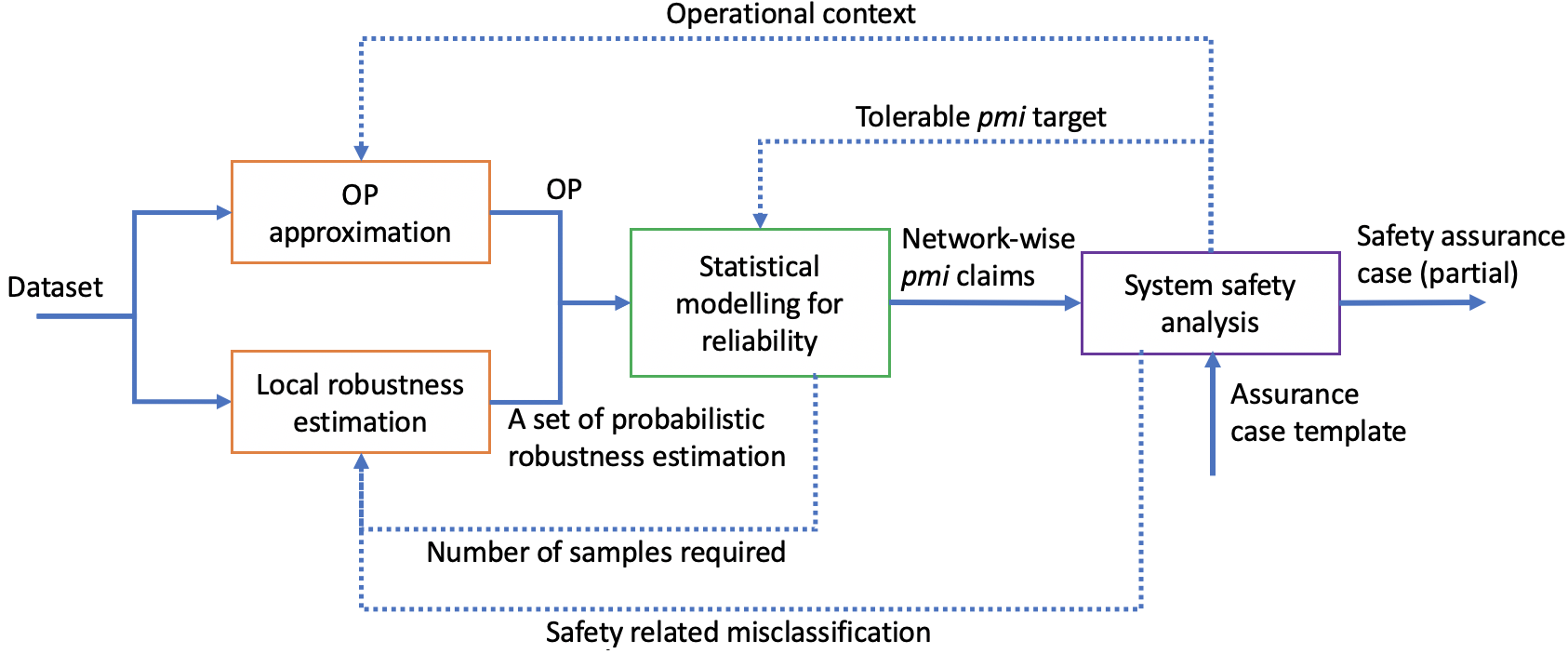
Figure 4. Overview of the proposed assurance framework. Blocks (at different levels are in different colours) represent major assurance activities corresponding to blocks ④, ⑤, ⑨ and ⑬ in Fig. 1. Solid lines show the inputs/output of blocks from lower levels to higher levels, while dotted lines show feedbacks.

4.1. Overview of an Assurance Case for LES

The proposed assurance case template is shown in Fig. 5, which is an overview of some top-level arguments and eight supporting CAE sub-cases. It also highlights the main focus of this work—a RAM for the ML component with its probabilistic safety arguments—and all its required supporting analysis to derive the reliability requirements of the low-level ML functionalities. It shows how various kinds of safety and reliability analysis/modelling methods are combined and structured to support our top-level claim TLC1—the LES S is acceptably safe. Additional information for the top claim should be provided (as for any safety case), describing the system S in detail and the target operational environments. The term “acceptably safe” is abstract and vague, thus we substitute it with TLC2 that all safety requirements R are satisfied. This substitution CAE-block/argument needs to be supported by a side-claim TLSC1 explaining why satisfying the set of requirements R implies S is safe enough.

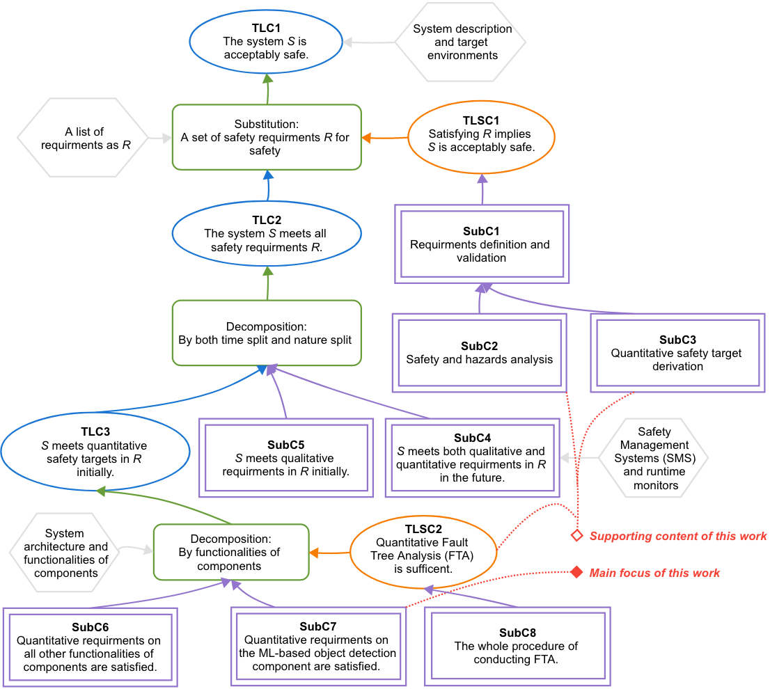
Figure 5. Overview of the proposed safety case template for LES, highlighting the main focus and supporting content of this work.

To argue for TLSC1, we refer to the template proposed by (Bloomfield et al., 2021, Chap. 5) as our sub-case SubC1. Essentially, in SubC1, we argue R is: (i) well-defined (e.g., verifiable, consistent, unambiguous, traceable, etc); (ii) complete that covers all sources (e.g., from hazard analysis and domain-specific safety standards and legislation); and (iii) valid, according to some common risk acceptance criteria/principles in safety regulations of different countries/domains, e.g., ALARP (As Low As Reasonably Practicable). Without repeating the content of (Bloomfield et al., 2021), we only highlight the parts directly supporting the main focus of this work (via the procedure in Fig. 6), which are hazard identification (SubC2) and derivation of quantitative safety target (SubC3).

Similar to (Bloomfield et al., 2021), we use a decomposition CAE-block/argument to support TLC2. But, in addition to time-split, we also split the claim by the qualitative and quantitative nature, since the main focus of this work, SubC7, concerns the probabilistic reliability modelling of ML components. Further decomposition of the whole system’s quantitative requirements into functionalities of individual components (TCL3) is non-trivial, for which we utilise quantitative FTA. The decomposition requires a side-claim on the sufficiency of the FTA study TLSC2. A comprehensive development SubC8 for TLSC2 is out of the scope of this work, while we illustrate the gist and an example of the method in later sections. Finally, we reach the main focus of this work SubC7 and will develop the full sub-case for it in Appendix E.

4.2. Deriving Quantitative Requirements for ML Components

In this work we are mainly developing low-level probabilistic safety arguments, based on the dedicated RAM for ML components developed in Section 5. An inevitable question is, how to quantitatively determine the tolerable and acceptable risk levels of the ML components? Normally the answer involves a series of well-established safety analysis methods that systematically breaks down the whole-system level risk to low-level components, considering the system architecture (Littlewood and Rushby, 2012; Zhao et al., 2020a). While, the whole-system level risk is determined on a case by case basis through the application of principles and criteria required by the safety regulations extant in the different countries/domains. To align with this best practice, we propose the procedure articulated in Fig. 6, whose major steps correspond to the supporting sub-cases SubC2, SubC3 and SubC8.

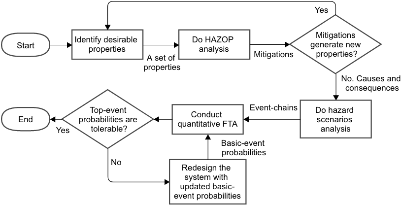
Figure 6. The workflow of combining HAZOP and quantitative FTA to derive probabilities of basic-events of components.

In Fig. 6, for the given LES, we first identify a set of safety properties that are desirable to stakeholders. Then, a HAZOP analysis is conducted, based on deviations of those properties, to systematically identify hazards (and their causes, consequences, and mitigations). New safety properties may be introduced by the mitigations identified by HAZOP, thus HAZOP is conducted in an iterative manner that forms the first loop in Fig. 6.

Then, we leverage the HAZOP results to do hazard scenario modelling, inspired by (Guo and Kang, 2015), so that we may combine HAZOP and FTA later on. Usually, as noted in (Guo and Kang, 2015), a property deviation can have several causes and different consequences in HAZOP analysis. It is complicated and difficult to directly convert HAZOP results into fault trees. Thus, hazard scenario modelling is needed to explicitly link the initial events (causes) to the final events (consequences) with a chain of intermediate events. Such event-chains facilitate the construction of fault trees, specifically in three steps:

• The initial events (causes) may or may not be further decomposed at even lower-level sub-functionalities of components to determine the root causes, which are used as basic events (BE) in FTA. Thus, BEs are typically failure events of software/hardware components, e.g., different types of misclassifications, failures in different modes of a propeller.

• Adding a specific logic gate among all intermediate events (IE) on the same level, which models how failures are propagated, tolerated and/or compounded throughout the system architecture.

• Final events (consequences) are used as top events (TE) of the FTA. In other words, TEs are violations of system-level safety properties.

Upon establishing the fault trees, conventional quantitative FTA can be performed to propagate probabilities of BEs to the TE probability, or, reversely, to allocate/break-down TE probability to BEs. What-if calculations and sensitivity analysis are expected to find the most practical solution of BE probabilities that makes the required TE risk tolerable. Then the practical solution for the BE associated with the ML component of our interest becomes our target reliability claims for which we develop probabilistic safety arguments. Notably, the ML component may need several rounds of retraining/fine-tuning to achieve the required level of reliability. This forms part of the second iterative loop in Fig. 6. We refer readers to (Zhao et al., 2021b) for a detailed description on this debug-retrain-assess loop for ML software.

Finally, the problem boils down to (i) how to derive the system-level quantitative safety target, i.e., assigning probabilities for those TEs of the fault trees; and (ii) how to demonstrate the component-level reliability is satisfied, i.e., assessing the BE probabilities for components based on evidence. We address the second question in the next section, while the first question is essentially “how safe is safe enough?”, for which the general answer depends on the existing regulation/certification principles/standards of different countries and industry domains. Unfortunately, existing safety standards cannot be applied on LES, and revisions are still ongoing. Therefore, we currently do not have a commonly acknowledged practice that can be easily applied to certify or regulate LES (Bloomfield et al., 2019; Kläs et al., 2021). That said, emerging studies on assuring/assessing the safety and reliability of AI and autonomous systems have borrowed ideas from existing regulation principles on risk acceptability and tolerability, to name a few:

• As Low As Reasonably Practicable (ALARP): ALARP states that the residual risk after the application of safety measures should be as low as reasonably practicable. The notion of being reasonably practicable relates to the cost and level of effort to reduce risk further. It originally arises from UK legislation and is now applied in many domains like nuclear energy.

• GALE: is a principle required by French law for railway safety, which indicates the new technical system shall be at least as safe as comparable existing ones.

• Substantially Equivalent (SE): similar to GALE; new medical devices in the US must be demonstrated to be substantially equivalent to a device already on the market. This is required by the U.S. Food & Drug Administration (FDA).

• Minimum Endogenous Mortality (MEM): MEM states that a new system should not lead to a significant increase in the risk exposure for a population with the lowest endogenous mortality. For instance, the rate of natural deaths is a reference point for acceptability.

While a complete list of all principles and comparisons between them are beyond the scope of this work, we believe that the common trend is that, for many LES, a promising way of determining the system-level quantitative safety target is to argue the acceptable/tolerable risk over the average human-performance. For instance, self-driving cars’ targets of being as safe as or two-magnitude safer than human-drivers (in terms of metrics like fatalities per mile) are studied in (Kalra and Paddock, 2016; Zhao et al., 2020c; Liu et al., 2019). In (Picardi et al., 2019), human-doctors’ performance is used as the benchmark in arguing the safety of ML-based medical diagnosis systems.

In summary, we are only presenting the essential steps of combining HAZOP and quantitative FTA via hazard scenario modelling to derive component-level reliability requirements from whole system-level safety targets, while each of those steps with concrete examples can be found in Section 6 as part of the AUV case study.

5. Modelling the Reliability of ML Classifiers

5.1. A Running Example of a Synthetic Dataset

To better demonstrate our RAM, we take the Challenge of AI Dependability Assessment raised by Siemens Mobility as a running example. The challenge is to firstly train an ML model to classify a dataset generated on the unit square $[0,1]^{2}$ according to some unknown distribution (essentially the unknown OP). The collected data-points (training set) are shown in Fig. 7-lhs, in which each point is a tuple of two numbers between 0 and 1 (thus called a “2D-point”). We then need to build a RAM to claim an upper bound on the probability that the next random point is misclassified, i.e., the pmi. If the 2D-points represent traffic lights, then we have 2 types of misclassifications—safety-critical ones, when a red data-point is labelled green, and performance related ones otherwise. For brevity, we consider both types of misclassifications here, while our RAM can cope with sub-types of misclassifications.

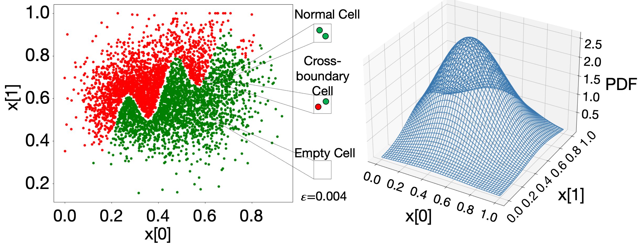
Figure 7. The 2D-point dataset (lhs), and its approximated OP (rhs).

5.2. The Proposed RAM

Principles and Main Steps of the RAM

Inspired by (Pietrantuono et al., 2020), our RAM first partitions the input domain into $m$ small cells, subject to the $r$-separation property. Then, for each cell $c_{i}$ (and its ground truth label $y_{i}$), we estimate:

(3) $$\lambda_{i} :=1-R_{{\mathcal{M}}}(c_{i},y_{i})\quad\mbox{and}\quad\mathsf{Op}_{i}:=\int_{x\in c_{i}}\mathsf{Op}(x)\mathop{}\!\mathrm{d}{x}\ ,$$

which are the unastuteness and pooled OP of the cell $c_{i}$ respectively—we introduce estimators for both later. Eqn. (1) can then be written as the weighted sum of the cell-wise unastuteness (i.e., the conditional pmi of each cell), where the weights are the pooled OP of the cells:

(4) $$\lambda=\sum_{i=1}^{m}\mathsf{Op}_{i}\lambda_{i}$$

Eqn. (4) captures the essence of our RAM—it shows clearly how we incorporate the OP information and the robustness evidence to claim reliability. This reduces the problem to: (i) how to obtain the estimates on those $\lambda_{i}$s and $\mathsf{Op}_{i}$s and (ii) how to measure and propagate the uncertainties in the estimates. These two questions are challenging. To name a few, for the first question: estimating $\lambda_{i}$ requires to determine the ground truth label of cell $i$; and estimating $\mathsf{Op}_{i}$s may require a large amount of operational data. For the second question, the fact that all estimators are imperfect entails that they need a measure of trust (e.g., the variance of a point estimate), which may not be easy to derive.

In what follows, by referring to the running example, we proceed in four main steps: (i) partition the input space into cells; (ii) approximate the OP of cells (the $\mathsf{Op}_{i}$s); (iii) evaluate the unastuteness of these cells (the $\lambda_{i}$s); and (iv) “assemble” all cell-wise estimates for $\lambda$ in a way that estimation uncertainties are propagated and compounded.

Step 1: Partition of the Input Domain $\mathcal{X}$

As per Remark 2, the astuteness evaluation of a cell requires its ground truth label. To leverage the $r$-separation property and the later Assumption 3, we partition the input space by choosing a cell radius $\epsilon$ so that $\epsilon<r$. Although we concur with Remark 3 (first observed by (Yang et al., 2020)) and believe that there should exist an $r$-stable ground truth (which means that the ground truth is stable in such a cell) for any real-world ML classification applications, it is hard to estimate such an $r$ (denoted by $\hat{r}$) and the best we can do is to assume:

Assumption 1.

There is a $r$-stable ground truth (as a corollary of Remark 3) for any real-world classification problems, and the $r$ parameter can be sufficiently estimated from the existing dataset.

That said, in the running example, we get $\hat{r}=0.004013$ by iteratively calculating the minimum distance of different labels. Then we choose a cell radius $\epsilon$, which is smaller than $\hat{r}$—we choose $\epsilon=0.004$. With this value, we partition the unit square $\mathcal{X}$ into $250\times 250$ cells.

Step 2: Cell OP Approximation

Given a dataset $(X,Y)$, we estimate the pooled OP of cell $c_{i}$ to get ${\mathbb{E}}[\mathsf{Op}_{i}]$ and ${\mathbb{V}}[\mathsf{Op}_{i}]$. We use the well-established Kernel Density Estimation (KDE) to fit a $\widehat{\mathsf{Op}}(x)$ to approximate the OP.

Assumption 2.

The given dataset $(X,Y)$ is collected and sampled based on the OP, and thus statistically represents the OP.

This assumption may not hold in practice: training data is normally collected in a balanced way, since the ML model is expected to perform well in all categories of inputs, especially when the OP is unknown at the time of training and/or expected to change in future. Although our model can relax this assumption in various ways (discussed in Section 7), we adopt it for brevity in demonstrating the running example.

Given a set of (unlabelled) data-points $(X_{1},\dots,X_{n})$ from the dataset $(X,Y)$, KDE then yields

(5) $$\widehat{\mathsf{Op}}(x)=\frac{1}{nh}\sum_{j=1}^{n}K(\frac{x-X_{j}}{h})\ ,$$

where $K$ is the kernel function (e.g. Gaussian or exponential kernels), and $h>0$ is a smoothing parameter, called the bandwidth, cf. (Silverman, 1986) for guidelines on tuning $h$. The approximated OP is shown in Fig. 7-rhs.

Since our cells are small and all equal size, instead of calculating $\int_{x\in c_{i}}\widehat{\mathsf{Op}}(x)dx$, we may approximate $\mathsf{Op}_{i}$ as

(6) $$\widehat{\mathsf{Op}}_{i}=\widehat{\mathsf{Op}}\left(x_{c_{i}}\right)v_{c}$$

where $\widehat{\mathsf{Op}}(x_{c_{i}})$ is the probability density at the cell’s central point $x_{c_{i}}$, and $v_{c}$ is the constant cell volume ($0.000016$ in the running example).

Now if we introduce new variables $W_{j}=\frac{1}{h}K(\frac{x-X_{j}}{h})$, the KDE evaluated at $x$ is actually the sample mean of $W_{1},\dots,W_{n}$. Then by invoking the Central Limiting Theorem (CLT), we have $\widehat{\mathsf{Op}}(x)\sim\mathcal{N}(\mu_{W},\frac{\sigma_{W}^{2}}{n})$, where the mean is exactly the value from Eqn. (5), while the variance of $\widehat{\mathsf{Op}}(x)$ is a known result of:

(7) $${\mathbb{V}}[\widehat{\mathsf{Op}}(x)] =\frac{f(x)\int K^{2}(u)du}{nh}+O(\frac{1}{nh})\approx\hat{\sigma}^{2}_{B}(x)\ ,$$

where the last step of Eqn. (7) says that ${\mathbb{V}}[\widehat{\mathsf{Op}}(x)]$ can be approximated using a bootstrap variance $\hat{\sigma}^{2}_{B}(x)$ (Chen, 2017) (cf. Appendix A for details).

Upon establishing Eqn.s (5) and (7), together with Eqn. (6), we know for a given cell $c_{i}$ (and its central point $x_{c_{i}}$):

(8) $${\mathbb{E}}[\mathsf{Op}_{i}]=v_{c}{\mathbb{E}}[\widehat{\mathsf{Op}}(x_{c_{i}})],\quad{\mathbb{V}}[\mathsf{Op}_{i}]=v_{c}^{2}{\mathbb{V}}[\widehat{\mathsf{Op}}(x_{c_{i}})]\ ,$$

which are the OP estimates of this cell.

Step 3: Cell Astuteness Evaluation

As a corollary of Remark 3 and Assumption 1, we may confidently assume:

Assumption 3.

If the radius of $c_{i}$ is smaller than $r$, all data-points in the cell $c_{i}$ share a single ground truth label.

Now, to determine such ground truth label of a cell $c_{i}$, we can classify our cells into three types:

• Normal cells: a normal cell contains data-points from the existing dataset. These data-points from a single cell are sharing a same ground truth label, which is then determined as the ground truth label of the cell.

• Empty cells: a cell is “empty” in the sense that it contains no data-points from the dataset of already collected data. Some of the empty cells will eventually become non-empty as more future operational data being collected, while most of them will remain empty forever—once cells are sufficiently small, only a small share of cells will refer to physically plausible images, and even fewer are possible in a given application. For simplicity, we do not further distinguish these two types of empty cells in this paper.

  Due to the lack of data, it is hard to determine an empty cell’s ground truth. For now, we do voting based on labels predicted (by the ML model) for random samples from the cell, making the following assumption.

  Assumption 4.

  The accuracy of the ML model is better than a classifier doing random classifications in any given cell.

  This assumption essentially relates to the oracle problem of ML testing, for which we believe that recent efforts (e.g. (Guerriero, 2020)) and future research may relax it.

• Cross-boundary cells: our estimate of $r$ based on the existing dataset is normally imperfect, e.g., due to noise in the dataset and the dataset size is not large enough. Thus, we may still observe data-points with different labels in a single cell (especially when new operational data with labels is collected). Such cells are crossing the classification boundary. If our estimate on $r$ is sufficiently accurate, they will be very rare. Without the need to determine the ground truth label of a cross boundary cell, we simply and conservatively set the cell unastuteness to 1.

So far, the problem is reduced to: given a normal or empty cell $c_{i}$ with the known ground truth label $y_{i}$, evaluate the misclassification probability upon a random input $x\in c_{i}$, ${\mathbb{E}}[{\lambda_{i}}]$, and its variance ${\mathbb{V}}[{\lambda_{i}}]$. This is essentially a statistical problem that has been studied in (Webb et al., 2019) using Multilevel Splitting Sampling, while we use the Simple Monte Carlo (SMC) method for brevity in the running example:

$$\hat{\lambda}_{i}=\frac{1}{n}\sum_{j=1}^{n}I_{\{M(x_{j})\neq y_{i}\}}$$

The CLT tells us $\hat{\lambda}_{i}\sim\mathcal{N}(\mu,\frac{\sigma^{2}}{n})$ when $n$ is large, where $\mu$ and $\sigma^{2}$ are the population mean and variance of $I_{\{{\mathcal{M}}(x_{j})\neq y_{i}\}}$. They can be approximated with sample mean $\hat{\mu}_{n}$ and sample variance $\hat{\sigma}_{n}^{2}/n$, respectively. Finally, we get

(9) $${\mathbb{E}}[{\lambda_{i}}] =\hat{\mu}_{n}=\frac{1}{n}\sum_{j=1}^{n}I_{\{{\mathcal{M}}(x_{j})\neq y_{i}\}}$$

(10) $${\mathbb{V}}[{\lambda_{i}}] =\frac{\hat{\sigma}_{n}^{2}}{n}=\frac{1}{(n-1)n}\sum_{j=1}^{n}(I_{\{{\mathcal{M}}(x_{j})\neq y_{i}\}}-\hat{\mu}_{n})^{2}$$

Notably, to solve the above statistical problem with sampling methods, we need to assume how the inputs in the cell are distributed, i.e., a distribution for the conditional OP $\mathsf{Op}(x\mid x\in c_{i})$. Without loss of generality, we assume:

Assumption 5.

The inputs in a small region like a cell are uniformly distributed.

This assumption is not uncommon (e.g., it is made in (Webb et al., 2019; Weng et al., 2019)) and can be replaced by other distributions, provided there is supporting evidence for such a change.

Step 4: Assembling of the Cell-Wise Estimates

Eqn. (4) represents an ideal case in which we know those $\lambda_{i}$s and $\mathsf{Op}_{i}$s with certainty. In practice, we can only estimate them with imperfect estimators yielding, e.g., a point estimate with variance capturing the measure of trust. To assemble the estimates of $\lambda_{i}$s and $\mathsf{Op}_{i}$s to get the estimates on $\lambda$, and also to propagate the confidence in those estimates, we assume:

Assumption 6.

All $\lambda_{i}$s and $\mathsf{Op}_{i}$s are independent unknown variables under estimations.

Then, the estimate of $\lambda$ and its variance are:

(11) $${\mathbb{E}}[\lambda] =\sum_{i=1}^{m}{\mathbb{E}}[\lambda_{i}\mathsf{Op}_{i}]=\sum_{i=1}^{m}{\mathbb{E}}[\lambda_{i}]{\mathbb{E}}[\mathsf{Op}_{i}]$$

(12) $${\mathbb{V}}[\lambda] =\sum_{i=1}^{m}{\mathbb{V}}[\lambda_{i}\mathsf{Op}_{i}]=\sum_{i=1}^{m}{\mathbb{E}}[\lambda_{i}]^{2}{\mathbb{V}}{[\mathsf{Op}_{i}]}+{\mathbb{E}}[\mathsf{Op}_{i}]^{2}{\mathbb{V}}[\lambda_{i}]+{\mathbb{V}}[\lambda_{i}]{\mathbb{V}}[\mathsf{Op}_{i}]$$

Note, for the variance, the covariance terms are dropped due to the independence assumption.

Depending on the specific estimators adopted, certain parametric families of the distribution of $\lambda$ can be assumed, from which any quantile of interest (e.g., 95%) can be derived as our confidence bound in reliability. For the running example, we might assume $\lambda\sim\mathcal{N}({\mathbb{E}}[\lambda],{\mathbb{V}}[\lambda])$ as an approximation by invoking the (generalised) CLT . Then, an upper bound with $1-\alpha$ confidence is

(13) $$\mathit{Ub}_{1-\alpha}={\mathbb{E}}[\lambda]+z_{1-\alpha}\sqrt{{\mathbb{V}}[\lambda]}\ ,$$

where $Pr(Z\leq z_{1-\alpha})=1-\alpha$, and $Z\sim\mathcal{N}(0,1)$ is a standard normal distribution.

Complexity Analysis on RAM

The computation complexity of RAM mainly comes from the estimation of $\lambda_{i}$ and $\mathsf{Op}_{i}$. For each cell $i$, the SMC requires simulation of $n_{1}$ samples, while $\mathsf{Op}_{i}$ is estimated by KDE, trained with $n_{2}$ collected operational data. The complexity of cell-wise estimation is $\mathcal{O}(n_{1}+n_{2})$. To get the final estimation of DL model’s $\lambda$, we assemble $m$ cells’ estimates. This results in the complexity of RAM being $\mathcal{O}(m*(n_{1}+n_{2}))$.

5.3. Extension to High-Dimensional Dataset

In order to better convey the principles and main steps of our proposed RAM, we have demonstrated a “low-dimensional” version of our RAM which is tailored for the running example (a synthetic 2D-dataset). However, real-world applications normally involve high-dimensional data like images, exposing the presented “low-dimensional” RAM to scalability challenges. In this section, we investigate how to extend our RAM for high-dimensional data, and take a few practical solutions to tackle the scalability issues raised by “the curse of dimensionality”.

Approximating the OP in the Latent Feature Space Instead of the Input Pixel Space

The number of cells yielded by the previously discussed way of partitioning the input domain (pixel space) is exponential in the dimensionality of data. Thus, it is hard to accurately approximate the OP due to the relatively sparse data collected: the number of cells is usually significantly larger than the number of observations made. However, for real-world data (say an image), what really determines the label is its features rather than the pixels. Thus, we envisage some latent space, e.g. compressed by Variational Auto-Encoders (VAE), that captures only the feature-wise information; this latent space can be explored for high-dimensional data. That is, instead of approximating the OP in the input pixel space, we (i) first encode/project each data-point into the compressed latent space, reducing its dimensionality, (ii) then fit a “latent space OP” with KDE based on the compressed dataset, and (iii) finally “map” data-points (paired with the learnt OP) in the latent space back to the input space.

Remark 4 (mapping between feature and pixel spaces).

Depending on which data compression technique we use and how the “decoder” works, the “map” action may vary case by case. For the VAE adopted in our work, we decode one point from the latent space as a “clean” image (with only feature-wise information), and then add perturbations to generate a norm ball (with a size determined by the $r$-separation distance, cf. Remark 3) in the input pixel space.

Applying Efficient Multivariate KDE for Cell OP Approximation

We may encounter technical challenges when fitting the PDF from high-dimensional datasets. There are two known major challenges when applying multivariate KDE to high-dimensional data: i) the choice of bandwidth $H$ represents the covariance matrix that mostly impacts the estimation accuracy; and ii) scalability issues in terms of storing intermediate data structure (e.g., data-points in hash-tables) and querying times made when estimating the density at a given input. For the first challenge, the optimal calculation of the bandwidth matrix can refer to some rule of thumb (Silverman, 1986; Scott, 2015) and the cross-validation (Bergstra and Bengio, 2012). There is also dedicated research on improving the efficiency of multivariate KDE, e.g., (Backurs et al., 2019) presents a framework for multivariate KDE in provably sub-linear query time with linear space and linear pre-processing time to the dimensions.

Applying Efficient Estimators for Cell Robustness

We have demonstrated the use of SMC to evaluate cell robustness in our running example. It is known that SMC is not computationally efficient to estimate rare-events, such as AE s in the high-dimensional space of a robust ML model. We therefore need more advanced and efficient sampling approaches that are designed for rare-events to satisfy our need. We notice that the Adaptive Multi-level Splitting method has been retrofitted in (Webb et al., 2019) to statistically estimate the model’s local robustness, which can be (and indeed has been) applied in our later experiments for image datasets. In addition to statistical approaches, formal method based verification techniques might also be applied to assess a cell’s pmi, e.g., (Huang et al., 2017). They provide formal guarantees on whether or not the ML model will misclassify any input inside a small region. Such “robust region” proved by formal methods is normally smaller than our cells, in which case the $\hat{\lambda}_{i}$ can be conservatively set as the proportion of the robust region covered in cell $c_{i}$ (under Assumption 5).

Assembling a Limited Number of Cell-Wise Estimates with Informed Uncertainty

The number of cells yielded by current way of partitioning the input domain is exponential to the dimensionality of data, thus it is impossible to explore all cells for high-dimensional data as we did for the running example. We may have to limit the number of cells under robustness evaluation due to the limited budget in practice. Consequently, in the final “assembling” step of our RAM, we can only assemble a limited number of cells, say $k$, instead of all $m$ cells. In this case, we refer to the estimator designed for weighted average based on samples (Bevington et al., 1993). Specifically, we proceed as what follows:

• Based on the collected dataset with $n$ data-points, the OP is approximated in a latent space, which is compressed by VAE. Then we may obtain a set of $n$ norm balls (paired with their OP) after mapping the compressed dataset to the input space (cf. Remark 4) as the sample frame.

• We define weight $w_{i}$ for each of the $n$ norm balls according to their approximated OP, $w_{i}:={\mathbb{E}}[\mathsf{Op}_{i}]$.

• Given a budget that we can only evaluate the robustness of $k$ norm balls, $k$ samples are randomly selected (with replacement) and fed into the robustness estimator to get ${\mathbb{E}}[\lambda_{i}]$.

• We may invoke the unbiased estimator for weighted average (Bevington et al., 1993, Chapter 4) as

  (14) $${\mathbb{E}}[\lambda] =\frac{\sum_{i=1}^{k}w_{i}{\mathbb{E}}[\lambda_{i}]}{\sum_{i=1}^{k}w_{i}}\ \mbox{and}$$

  (15) $${\mathbb{V}}[\lambda] =\frac{1}{k-1}\left(\frac{\sum_{i=1}^{k}w_{i}\left({\mathbb{E}}[\lambda_{i}]\right)^{2}}{\sum_{i=1}^{k}w_{i}}-({\mathbb{E}}[\lambda])^{2}\right)\ .$$

  Moreover, a confidence upper bound of interest can be derived from Eqn. (13).

Note that there is no variance terms of $\lambda_{i}$ and $\mathsf{Op}_{i}$ in Eqn.s (14) and (15), implying the following assumption:

Assumption 7.

The uncertainty informed by Eqn. (15) is sourced from the sampling of $k$ norm balls, which is assumed to be the major source of uncertainty. This makes the uncertainties contributed by the robustness and OP estimators (i.e. the variance terms of $\lambda_{i}$ and $\mathsf{Op}_{i}$) negligible.

Complexity Analysis on RAM Extension to High-Dimensional Dataset

For high dimensional data, RAM still adopts the KDE, fitted with $n_{2}$ operational data projected into low dimensional latent feature space. The main difference is the use of more efficient estimators for cell robustness. We refer to the Adaptive Multi-level Splitting method, an advanced Monte Carlo Simulation, that has been used for local robustness estimation in (Webb et al., 2019) and our experiments. If SMC requires the number of simulations at the order of $n_{1}$ for accurate estimation of rare events with probability $1/n_{1}$ (while omitting the coefficient, cf. (Littlewood and Strigini, 1993) for detailed analytical results), the Adaptive Multi-level Splitting method (cf. (Webb et al., 2019) for more algorithm details) utilises the product of conditional probability with $\log{}n_{1}$ levels (the quantile $\rho$ is normally set to 0.1). If $n_{3}$ samples are simulated by SMC for calculating each conditional probability, the computation cost of Adaptive Multi-level Splitting method is $n_{3}\log{}n_{1}\ll n_{1}$. Finally, we invoke the weighted sampling of $k$ cells for cell-wise estimates assembling, the complexity of which is $\mathcal{O}(k*(n_{3}\log{}n_{1}+n_{2}))$.

5.4. Evaluation on the Proposed RAM

In addition to the running example, we conduct experiments on two more synthetic 2D-datasets, as shown in Fig. 8. They represent scenarios with relatively sparse and dense training data, respectively. Moreover, to gain insights on how to extend our RAM for high-dimensional datasets, we also conduct experiments on the popular MNIST and CIFAR10 datasets, as articulated in Section 5.3. All modelling details and results after applying our RAM on those datasets are summarised in Table 1, where we compare the testing error, Average Cell Unastuteness (ACU) defined by Definition 5.1, and our RAM results (of the mean ${\mathbb{E}}[\lambda]$, variance ${\mathbb{V}}[\lambda]$ and a 97.5% confidence upper bound $Ub_{97.5\%}$).

Definition 0 (ACU).

Stemmed from the Definition 2 and Remark 2, the unastuteness $\lambda_{i}$ of a region $c_{i}$ is consequently $1-R_{{\mathcal{M}}}(c_{i},y_{i})$ where $y_{i}$ is the ground truth label of $c_{i}$ (cf. Eqn. 3). Then we define the ACU of the ML model as:

(16) $$ACU:=\frac{1}{m}\sum_{i=1}^{m}\lambda_{i}$$

where $m$ is the total number of regions.

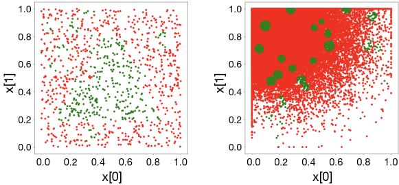
Figure 8. Synthetic datasets DS-1 (lhs) and DS-2 (rhs) representing relatively sparse and dense training data respectively.

Table 1. Modelling details & results of applying the RAM on five datasets. Time is in seconds per cell.

	train/test error	$r$-separation	radius $\epsilon$	# of cells	ACU	${\mathbb{E}}[\lambda]$	${\mathbb{V}}[\lambda]$	$Ub_{97.5\%}$	time
The run. exp.	0.0005/0.0180	0.004013	0.004	$250\times 250$	0.002982	0.004891	0.000004	0.004899	0.04
Synth. DS-1	0.0037/0.0800	0.004392	0.004	$250\times 250$	0.008025	0.008290	0.000014	0.008319	0.03
Synth. DS-2	0.0004/0.0079	0.002001	0.002	$500\times 500$	0.004739	0.005249	0.000002	0.005252	0.04
Norm. MNIST	0.0051/0.0235	0.369	0.300	$k$	Fig. 9(b)	Fig. 9(a)	Fig. 9(a)	Fig. 9(a)	0.43
Adv. MNIST	0.0173/0.0212	0.369	0.300	$k$	Fig. 9(d)	Fig. 9(c)	Fig. 9(c)	Fig. 9(c)	0.43
Norm. CIFAR10	0.0190/0.0854	0.106	0.100	$k$	Fig. 10(b)	Fig. 10(a)	Fig. 10(a)	Fig. 10(a)	6.74
Adv. CIFAR10	0.0013/0.1628	0.106	0.100	$k$	Fig. 10(d)	Fig. 10(c)	Fig. 10(c)	Fig. 10(c)	6.74

In the running example, we first observe that the ACU is much lower than the testing error, which means that the underlying ML model is a robust one. Since our RAM is largely based on the robustness evidence, its results are close to ACU, but not exactly the same because of the nonuniform OP, cf. Fig. 7-rhs.

Remark 5 (ACU is a special case of pmi).

When the OP is “flat” (uniformly distributed), ACU and our RAM result regarding pmi are equal, which can be seen from Eqn. 4 by setting all $\mathsf{Op}_{i}$s equally to $\frac{1}{m}$.

Moreover, from Fig. 7-lhs, we know that the classification boundary is near the middle of the unit square input space where misclassifications tend to happen (say, a “buggy area”), which is also the high density area on the OP. Thus, the contribution to unreliability from the “buggy area” is weighted higher by the OP, explaining why our RAM results are worse than the ACU. In contrast, because of the relatively “flat” OP for the DS-1 (cf. Fig. 8-lhs), our RAM result is very close to the ACU (cf. Remark 5). With more dense data in DS-2, the $r$-distance is much smaller and leads to smaller cell radius and more cells. Thanks to the rich data in this case, all three results (testing error, ACU, and the RAM) are more consistent than in the other two cases. We note that, given the nature of the three 2D-point datasets, ML models trained on them are much more robust than image datasets. This is why all ACU s are better than test errors, and our RAM finds a middle point representing reliability according to the OP. Later we apply the RAM on unrobust (by normal training) and robust (by adversarial training) ML models trained on image datasets, where the ACU s are worse and better than the test error, respectively; it confirms our aforementioned observations.

Figure 9. The mean, variance and 97.5% confidence upper bound of pmi and ACU as functions of $k$ sampled norm ball, estimated on MNIST dataset with normally and adversarially trained models.

Figure 10. The mean, variance and 97.5% confidence upper bound of pmi and ACU as functions of $k$ sampled norm ball, estimated on CIFAR10 dataset with normally and adversarially trained models.

Regarding the MNIST and CIFAR10 datasets, all the experiment codes for this running example are publicly available at https://github.com/havelhuang/ReAsDL, and the model details are presented in Appendix B.1. In this section, we first train VAE s on them and compress the datasets into the low dimensional latent spaces of VAE s with 8 and 16 dimensions, respectively. We then fit the compressed dataset with KDE to approximate the OP. Each compressed data-point is now associated with a weight representing its OP. Consequently, each norm ball in the pixel space that corresponds to the compressed data-point in the latent space (after the mapping, cf. Remark 4) is also weighted by the OP. Taking the computational cost into account—say only the astuteness evaluation on a limited number of $k$ norm balls is affordable—we do random sampling, invoke the estimator for weighted average Eqn.s (14) and (15). We training two DL models with normal training strategy and PGD-based adversarial training strategy (Madry et al., 2018), respectively, and plot our RAM results for both models as functions of $k$ in (a) and (c) of Figures 9 and 10. For comparison, we also plot the ACU results in (b) and (d) of Figures 9 and 10.

In Figures 9 and 10, we first observe that both the ACU results (after converging) of normally trained MNIST and CIFAR10 models are worse than their test errors (in Table 1), unveiling again the robustness issues of ML models when dealing with image datasets (while the ACU of CIFAR10 is even worse, given that CIFAR10 is indeed a generally harder dataset than MNIST). For MNIST, the mean pmi estimates are much lower than ACU, implying a very “unbalanced” distribution of weights (i.e. OP). Such unevenly distributed weights are also reflected in both, the oscillation of the variance and the relatively loose 97.5% confidence upper bound. On the other hand, the OP of CIFAR10 is flatter, resulting in closer estimates of pmi and ACU (Remark 5). For adversarially trained models, the robustness of which is improved significantly at the cost of accuracy drop shown in Table 1. It is still effective to reduce the $pmi$ and ACU of DL models.

In summary, for real-world image datasets, our RAM may effectively assess the robustness of the ML model and its generalisability based on the shape of its approximated OP, which is much more informative than either the test error or ACU alone. Finally, based on the RAM, templates of probabilistic arguments for reliability claims on ML components are developed, cf. Appendix E.

6. Case Studies

In this section, a case study based on a simulated AUV that performs survey and asset inspection missions is conducted. We first describe the scenario in which the mission is performed, details of the AUV under test, and how the simulator is implemented. Then, corresponding to Section 4, we exercise the proposed assurance activities for this AUV application, i.e., HAZOP, hazards scenarios modelling, FTA, and discussions on deriving the system-level quantitative safety target for this scenario. Finally, we apply our RAM on the image dataset collected from a large amount of statistical testing.

6.1. Scenario Design

AUV are increasingly adopted for marine science, offshore energy, and other industrial applications in order to increase productivity and effectiveness as well as to reduce human risks and offshore operation of crewed surface support vessels (Lane et al., 2016). However, the fact that AUVs frequently operate in close proximity to safety-critical assets (e.g., offshore oil rigs and wind turbines) for inspection, repair and maintenance tasks leads to challenges on the assurance of their reliability and safety, which motivates the choice of AUV as the object of our case study.

6.1.1. Mission Description and Identification of Mission Properties

Based on industrial use cases of autonomous underwater inspection, we define a test scenario for AUVs that need to operate autonomously and carry out a survey and asset inspection mission, in which an AUV follows several way-points and terminates with autonomous docking. During the mission, it needs to detect and recognise a set of underwater objects (such as oil pipelines and wind farm power cables) and inspect assets (i.e., objects) of interest, while avoiding obstacles and keeping the required safe distances to the assets.

Given the safety/business-critical mission, different stakeholders have their own interests on a specific set of hazards and safety elements. For instance, asset owners (e.g., wind farm operators) focus more on the safety and health of the assets that are scheduled to be inspected, whereas inspection service providers tend to have additional concerns regarding the safety and reliability of their inspection service and vehicles. In contrast, regulators and policy makers may be more interested in environmental and societal impacts that may arise when a failure unfortunately happens. By keeping these different safety concerns in mind, we identify a set of desirable mission properties, whose violation may lead to unsuccessful inspection missions, compromise the integrity of critical assets, or damage of the vehicle itself.

While numerous high-level mission properties are identified based on our engineering experience, references to publications (e.g., (Hereau et al., 2020)) and iterations of hazard analysis, we focus on a few that are instructive for the ML classification function in this article (cf. the project website for a complete list):

• No miss of key assets: the total number of correctly recognised assets/objects should be equal to the total number of assets that are required to be inspected during the mission.

• No collision: during the full mission, the AUV should avoid all obstacles perceived without collision.

• Safe distancing: once an asset is detected and recognised, the Euclidean distance between the AUV and the asset must be kept to be at least the defined minimal safe operating distance.

• Autonomous docking: safe and reliable docking to the docking cage.

Notably, such an initial set of desirable mission properties forms the starting point of our assurance activities, cf. Fig. 6 and Section 6.2.

6.1.2. The AUV Under Test

Hardware

Although we are only conducting experiments in simulators at this stage, our trained ML model can be easily deployed to real robots and the experiments are expected to be reproducible in real water tanks. Thus, we simulate the AUV in our laboratory—a customised BlueROV2, which has 4 vertical and 4 horizontal thrusters for 6 degrees of freedom motion. As shown in Fig. 11-lhs, it is equipped with a custom underwater stereo camera designed for underwater inspection. A Water Linked A50 Doppler Velocity Log (DVL) is installed for velocity estimation and control. The AUV also carries an Inertial Measurement Unit (IMU), a depth sensor and a Tritech Micron sonar. The AUV is extended with an on-board Nvidia Jetson Xavier GPU computer and a Raspberry Pi 4 embedded computer. An external PC can also be used for data communication, remote control, mission monitoring, and data visualisation of the AUV via its tether.

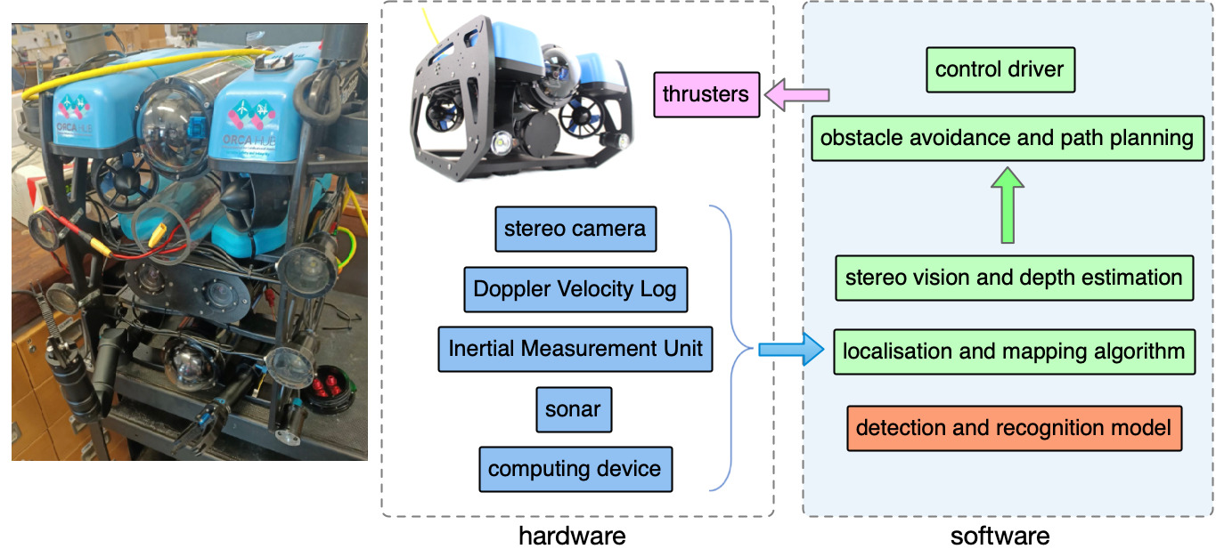
Figure 11. Hardware–software architecture & key modules for autonomous survey & inspection missions.

Software Architecture

With the hardware platform, we develop a software stack for underwater autonomy based on the Robot Operating System (ROS). The software modules that are relevant to the aforementioned AUV missions are (cf. Fig. 11):

• Sensor drivers. All sensors are connected to on-board computers via cables, and their software drivers are deployed to capture real-time sensing data.

• Stereo vision and depth estimation. This is to process stereo images by removing its distortion and enhancing its image quality for inspection. After rectifying stereo images, they are used for estimating depth maps that are used for 3D mapping and obstacle avoidance.

• Localisation and mapping algorithm. In order to navigate autonomously and carry out a mission, we need to localise the vehicle and build a map for navigation. We develop a graph optimisation based underwater simultaneous localisation and mapping system by fusing stereo vision, DVL, and IMU. It also builds a dense 3D reconstruction model of structures for geometric inspection.

• Detection and recognition model. This is one of the core modules for underwater inspection based on ML models. It is designed to detect and recognise objects of interest in real-time. Based on the properties of detected objects— in particular the underwater assets to inspect—the AUV makes decisions on visual data collection and inspection.

• Obstacle avoidance and path planning. The built 3D map and its depth estimation are used for path planning, considering obstacles perceived by the stereo vision. Specifically, a local trajectory path and its way-points are generated in the 3D operating space based on the 3D map built from the localisation and mapping algorithm. Next the computed way-point is passed to the control driver for trajectory and way-point following.

• Control driver. We have a back seat driver for autonomous operations, enabling the robot to operate as an AUV. Once the planned path and/or a way-point is received, a Proportional-Integral-Derivative (PID) based controller is used to drive the thrusters following the path and approaching to the way-point. The controller can also be replaced by a learning based adaptive controller. While the robot moves in the environment, it continues perceiving the surrounding scene and processing the data using the previous software modules.

ML Model Doing Object Detection

In this work, the state-of-the-art Yolo-v3 DL architecture (Redmon and Farhadi, 2018) is used for object detection. Its computational efficiency and real-time performance are both critical for its application for underwater robots, as they mostly have limited on-board computing resources and power. The inference of Yolo can be up to 100 frames per second. Yolo models are also open source and built using the C language and the library is officially supported by OpenCV, which makes its integration with other AUV systems not covered in this work straightforward. Most DL-based object detection methods are extensions of a simple classification network. The object detection network usually generates a set of proposal bounding boxes; they might contain an object of interest and are then fed to a classification network. The Yolov3 network is similar in operation to, and is based on, the darknet53 classification network.

The process of training the Yolo networks using the Darknet framework is similar to the training of most ML models, which includes data collection, model architecture implementation, and training. The framework consists of configuration files that can be set to match the number of object classes and other network parameters. Examples of training and testing data are described in Section 6.1.3 for simulated version of the model. The model training can be summarised by the following steps: i) define the number of object categories; ii) collect sufficient data samples for each category; iii) split the data into training and validation sets; and iv) use the Darknet software framework to train the model.

6.1.3. The Simulator

The simulator uses the popular Gazebo robotics simulator in combination with a simulator for underwater dynamics. The scenario models can be created/edited using Blender 3D software. We have designed the Ocean Systems Lab’s wave tank model (cf. Fig. 12-lhs) for the indoor simulated demo, using BlueROV2 within the simulation to test the scenarios. The wave tank model has the same dimension as our real tank.

Figure 12. A wave-tank for simulated testing and a simulated pool for collecting the training data.

To ensure that the model does not overfit the data, we have designed another scenario with a bigger pool for collecting the training data. The larger size allows for more distance between multiple objects, allowing both to broaden the set training scenarios and to make them more realistic. The simulated training environment is presented in Fig. 12-rhs.

Our simulator creates configuration files to define an automated path using Cartesian way-points for the vehicle to follow autonomously, which can be visualised using Rviz. The pink trajectory is the desirable path and the red arrows represent the vehicle poses following the path, cf. Fig. 13-lhs. There are six simulated objects in the water tank. They are a pipe, a gas tank, a gas canister, an oil barrel, a floating ball, and the docking cage, as shown in Fig. 13-rhs. The underwater vehicle needs to accurately and timely detect them during the mission. Notably, the mission is also subject to random noise factors, so that repeated missions will generate different data that is processed by the learning-enabled components.

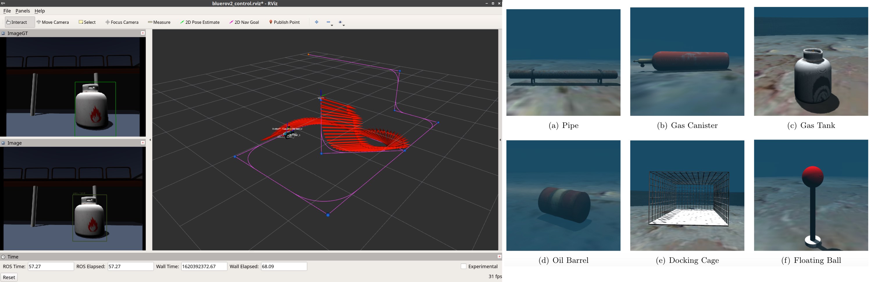
Figure 13. Simulated AUV missions following way-points and the six simulated objects.

6.2. Assurance Activities for the AUV

Hazard Analysis via HAZOP

Given the AUV system architecture (cf. Fig. 11) and control/data flow among the nodes, we conducted a HAZOP analysis that yields a complete version of Table 2 in (Qi et al., 2022). For this work, we only present partial HAZOP results and highlight a few hazards that are due to misclassification.

HAZOP item: node/flow	Process parameter or attribute	Guide-word	Cause	Consequence	Mitigation
flow from object detection to obstacle avoidance and path planning	data flow	too late	…	…	…
		…	…	…	…
	data value	wrong value	misclassification	erratic navigation; unsafe distance to assets; collision to assets; failed inspection.	acoustic guidance; minimum DL-classifier reliability for critical objects; maximum safe distance maintained if uncertain; …
		no value	…	…	…
		…	…	…	…
…	…	…	…	…	…

Table 2. Partial HAZOP results, highlighting the cause of misclassification (NB, entries of “…” are intentionally left blank, cf. (Qi et al., 2022) and our public project repository for a complete version).

Hazard Scenarios Modelling

Inspired by (Guo and Kang, 2015), we develop the hazard scenarios as chains of events that link the causes to consequences identified by HAZOP. Again, for illustration, a single event-chain is shown in Fig. 14, which propagates the event of misclassification on assets via the system architecture to the violation of mission property of keeping a safe distance to assets. Later, readers will see this event-chain forms one path of a fault tree in the FTA in Fig. 15.

Figure 14. An event-chain based on the hazard scenario modelling, linking causes to consequences.

Quantitative FTA

We first construct fault trees for each hazard (as TE) identified by HAZOP, by extending and combining (via logic gates) the IEs modelled by hazard scenario analysis. Each event-chain yielded by the hazard scenario analysis then forms one path in a fault tree. For instance, the event-chain of Fig. 14 eventually becomes the path of BE-0-1 $\rightarrow$ IE-1-1 $\rightarrow$ IE-2-2 $\rightarrow$ IE-3-2 $\rightarrow$ TE in Fig. 15. Finally, knowing the probabilities of BEs and logic gates allows for the calculation of the TE probability. As shown by the second iteration loop in Fig. 6, several rounds of what-if calculations, sensitivity analysis and updates of the components are expected to yield the most practical solution of BE probabilities that associates with a given tolerable risk of the TE.

Figure 15. A partial fault tree for the TE of loss of a safe distance to assets. NB, the “cloud” notation represents omitted sub-trees.

Deriving Quantitative System Safety Target

Based on the experience of relatively more developed safety-critical domains of AI, such as self-driving cars and medical devices (cf. Section 4.2 for some examples), we believe that referring to the average performance of human divers and/or human remote control operators is a promising way of determining the high-level quantitative safety target for our case of an AUV. It is presumed that, prior to the use of an AUV for assets inspection, human divers and remotely controlled robots need to conduct the task regularly. This is also similar to how the safety targets were developed in the civil aircraft sector where they refer to acceptable historical accident rates as the benchmark. In our case, referring to the human-divers/operators’ performance as a target for an AUV’s safety risk can be potentially impeded by the lack of historical/statistical data on such performance. Given the fact that ML for AUV is a relatively novel technique and still developing and transforming to its practical uses, an urgent lesson learnt for all AUV stakeholders (especially manufacturers, operators and end users) from this work is to collect and summarise such data.

6.3. Reliability Modelling of the AUV’s Classification Function

Details of the Yolo3 model trained in this case study is presented in Table 3, B.2. We adopt the practical solutions discussed in Section 5.3 to deal with the high dimensionality of the collected operational dataset (256*256*3) by first training a VAE model and compressing the dataset into a new space with a much lower dimensionality of 8. While training details of the VAE model are summarised in Table 4, four sets of examples are shown in Fig. 22, from which we can see that the reconstructed images are preserving the essential features of the objects (while blurring the less important background). We then choose a norm ball radius $\epsilon=0.06$ according to the $r$-separation distance and invoke the KDE and robustness estimator (Webb et al., 2019) for $k$ randomly selected norm balls. Individual estimates of the $k$ norm balls are then fed into the estimator for weighted average, Eqn.s (14) and (15). For comparison, we also calculate the ACU by assuming equal weights (i.e., a flat OP) in Eqn.s (14) and (15). Finally, the reliability claims on pmi and ACU are plotted as functions of $k$ in Fig. 16. Interpretation of the results is similar as before for CIFAR10, where the OP is also relatively flat. From the comparison results, it can be seen that the adversarial train can effectively improve the robustness of DL models and be captured by our RAM method.

Figure 16. The mean, variance and 97.5% confidence upper bound of AUV’s pmi and ACU as functions of $k$ sampled norm balls.

6.4. An Extended Case Study on Real World Unmanned Ground Vehicles

In this case study, we deployed a customised real-world UGV robot, named JACKAL, as shown in Fig. 17(a). A demo video is available on Youtube.

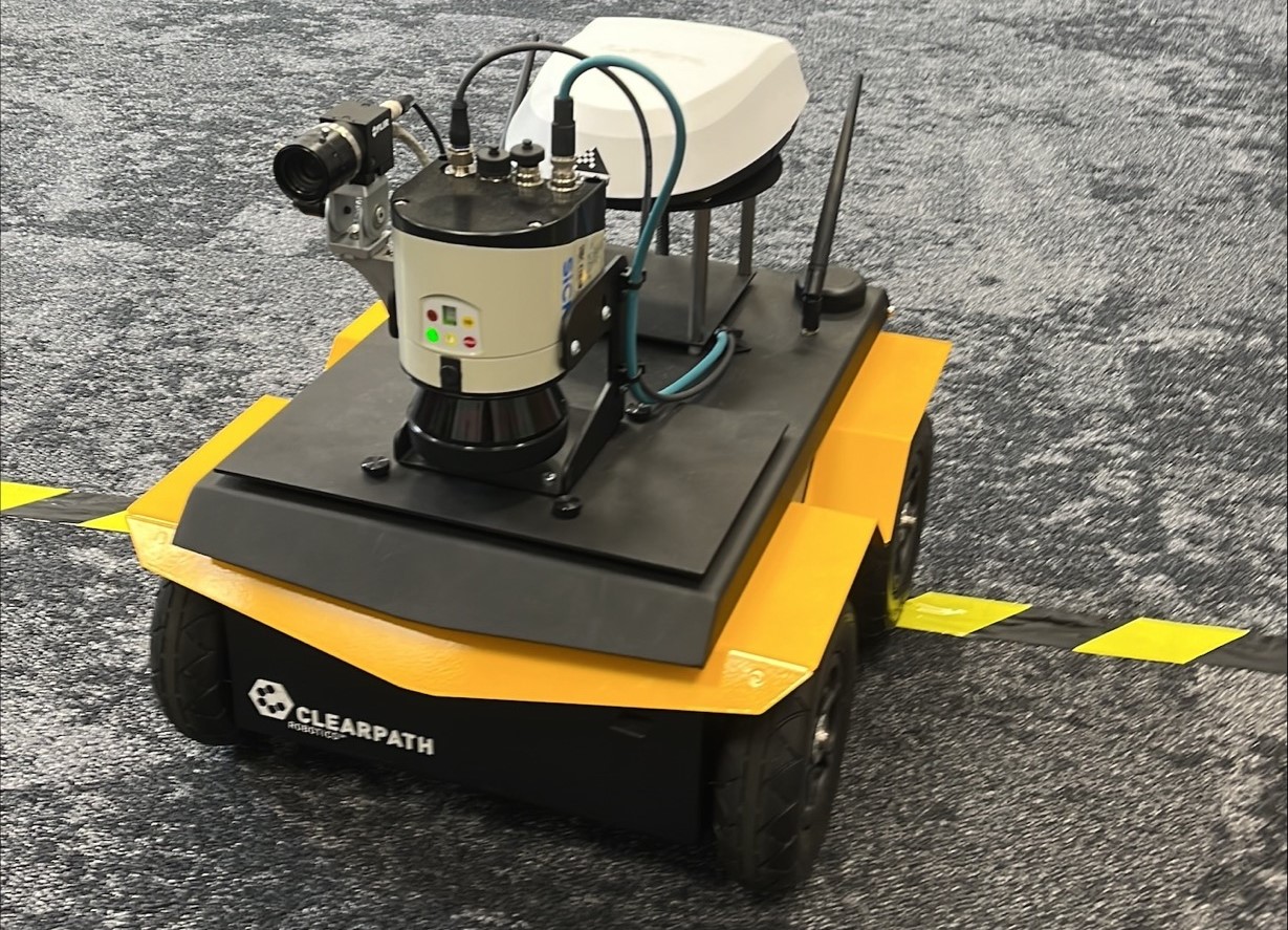
(a) Jackal Robot

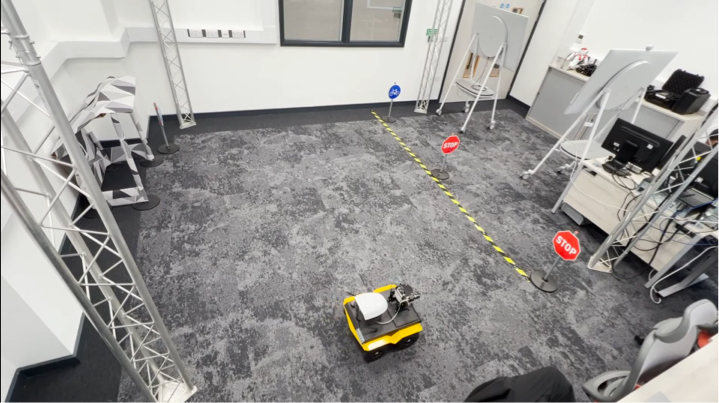
(b) Physical Environment

Figure 17. The UGV and its deployed environment.

Similar to the AUV case study, the mission of UGV case study is to detect the different traffic signs. In this experiment, we set 5 different labels, stop sign, park sign, cycle sign, cross sign and one-way sign. We trained a YOLOv3 model with normal training and adversarial training based on the same dataset. All the experiment settings and details are given about the evaluation of the RAM in Section B.2. The RAM results are described in the following parts.

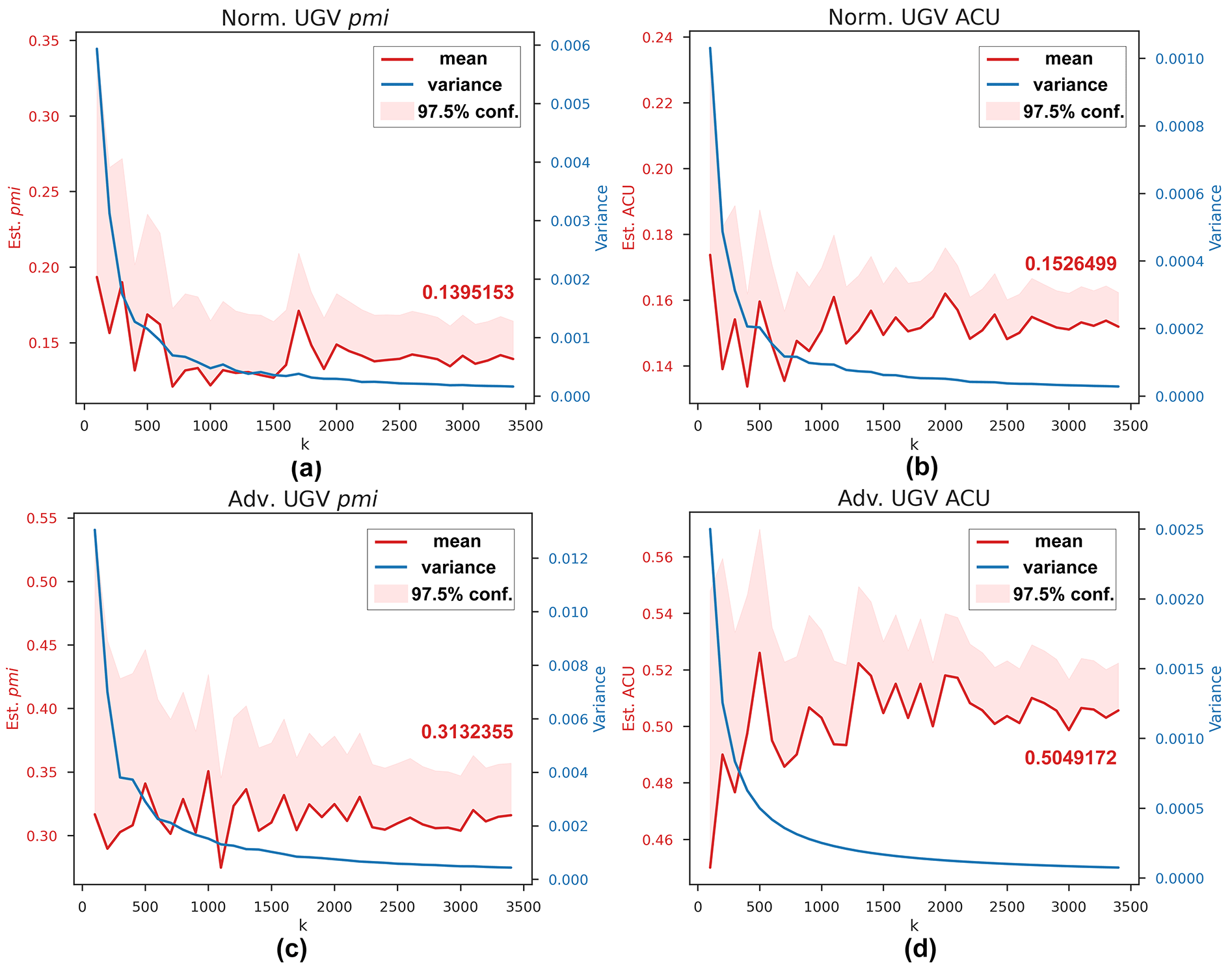
Figure 18. The mean, variance and 97.5% confidence upper bound of UGV’s pmi and ACU as functions of $k$ sampled norm balls.

As shown in Fig. 18, with the increasing amount of sampled data, the final assessment results are all converged with decreasing variance. Comparing sub-figures (a) and (b), or (c) and (d), we can find our $pmi$ evaluation is different from the ACU in consideration of the OP. In addition, we estimate $pmi$ and ACU on two models trained with different schemes. The train and test average precision (AP) are presented in Table 3. The adversarial training can improve the robustness of YOLO model at the cost of compromising the generalisation (indicated by mAP). The $pmi$ metric can be conceptually perceived as a product of “generalisation $\times$ robustness” (Zhao et al., 2021a). Although previous experiments for MNIST, CIFAR10 and AUV shows the effectiveness of adversarial training for improving DL model’s reliability by reducing the $pmi$, Fig. 18 displays the risk that adversarial training may potentially harm the reliability when there exists improper trade-off between generalisation and robustness. mAP for adversarially trained UGV model is significantly decreased from 0.98 to nearly 0.81, shown in Table 3. Too large drop-off of generalisation is disadvantageous to the reliability improvement. This motivates us to design new training schemes in the future towards more reliable DL models that are both robust and generalisable.

7. Discussion

7.1. Discussions on the Proposed RAM

In this section, we summarise the model assumptions made in our RAM, and discuss if/how they can be validated and which new assumptions and compromises in the solutions are needed to cope with real-world applications with high-dimensional data. Finally, we list the inherent difficulties of assessing ML reliability uncovered by our RAM.

$R$-Separation and its Estimation

Assumption 1 derives from Remark 3. We concur with (Yang et al., 2020) and believe that, for any real-world ML classification application where the inputs are data-points with “physical meanings”, there should always exist an $r$-stable ground truth. Such $r$-stable ground truth varies between applications, and the smaller the $r$ is, the harder the inherent difficulty of the classification problem becomes. This $r$ is therefore a difficulty indicator for the given classification problem. Indeed, it is hard to estimate the $r$ (either in the input pixel space nor the latent feature space)—the best we can do is to estimate it from the existing dataset. One way of solving the problem is to keep monitoring the $r$ estimates as more labelled data is collected, e.g. during operation, and to redo the cell partition when the estimated $r$ has changed significantly. Such a dynamic way of estimating $r$ can be supported by the concept of dynamic assurance cases (Asaadi et al., 2020b).

Approximation of the OP from Data

Assumption 2 says that the collected dataset statistically represents the OP, which may not hold for many practical reasons—e.g., when the future OP is uncertain at the training stage and data is therefore collected in a balanced way to perform well in all categories of inputs. Although we demonstrate our RAM under this assumption for simplicity, it can be relaxed for the following reasons. Any given dataset that differs from the OP requires a preprocessing step to synthesis a new “operational dataset” (representing the OP), e.g., by generative models, adding weights to data-points, etc. Indeed, such preprocessing step may require domain expert knowledge and/or historical data of similar products which is not an uncommon practice for traditional software (Smidts et al., 2014). That is, we try to fit a PDF over the input space from the “operational dataset”, and data-points in this set can be raw data generated from historical data of previous applications which can then be scaled based on domain expert knowledge and by adding new data from simulation/generative-models. Obtaining such an operational dataset is an application-specific engineering problem, and manageable thanks to the fact that it does not require manual labelling. Notably, the OP may also be approximated at runtime based on the data stream of operational data. Efficient KDE for data streams (Qahtan et al., 2017) can be used. If the OP was subject to sudden changes, change-point detectors like (Zhao et al., 2020b) should also be paired with the runtime estimator to robustly approximate the OP. Such dynamic way of estimating OP can also be supported by dynamic assurance cases (Asaadi et al., 2020b).

Determination of the Ground Truth of a Cell

Assumptions 3 and 4 are essentially on how to determine the ground truth label for a given cell, which relates to the oracle problem of testing ML software. While this still remains challenging, we partially solve it by leveraging the $r$-separation property. Thanks to $r$, it is easy to determine a cell’s ground truth when we see that it contains labelled data-points. However, for an empty cell, it is non-trivial. We assume the overall performance of the ML model is fairly good (e.g., better than a classifier doing random classifications), thus misclassifications within an empty cell are relatively rare events. We can determine the ground truth label of the cell by majority voting of predictions. Indeed, it is a strong assumption when there are some “failure regions” in the input space, within which the ML model performs really badly (even worse than random labelling). In this case, we need new mechanism to detect such “really bad failure regions” or spend more budget on, for example, asking humans to do the labelling.

Efficiency of Cell Robustness Evaluation

Although we only applied the two methods of SMC and (Webb et al., 2019) in our experiments to evaluate the local robustness, we believe that other statistical sampling methods designed for estimating the probability of rare-events could be used as well. Moreover, the cell robustness estimator in our RAM works in a “hot-swappable” manner: any new and more efficient estimator can easily be incorporated. Thus, despite being an important question, how to improve the efficiency of the robustness estimation for cells is beyond the scope of our RAM.

Conditional OP of a Cell

We assume that the distribution of inputs (the conditional OP) within each cell is uniform by Assumption 5. Although we conjecture that this is the common case due to the small size of cells (i.e., those very close/similar inputs within a small region are only subject to noise factors that can be modelled uniformly), the specific situation may vary; this requires justification in safety cases. For a real-world dataset, the conditional OP might represent certain distributions of “natural variations” (Zhong et al., 2021), e.g. lighting conditions, that obey certain distributions. Ideally, the conditional OP of cells should capture the distribution of such natural variations. Recent advance on measuring the naturalness/realisticness of AE s (Harel-Canada et al., 2020) relates to this assumption and may relax it.

Independent $\lambda_{i}$s and $\mathsf{Op}_{i}$s

As per Assumption 6, we assume all $\lambda_{i}$s and $\mathsf{Op}_{i}$s are independent when “assembling” their estimates via Eqn. (11) and deriving the variance via Eqn. (12). This assumption is largely for the mathematical tractability when propagating the confidence in individual estimates at the cell-level to the pmi. Although this independence assumption is hard to justify in practice, it is not unusual in reliability models that do partition, e.g., in (Pietrantuono et al., 2020; Miller et al., 1992). We believe that RAMs are still useful under this assumption, while we envisage that Bayesian estimators leveraging joint priors and conjugacy may relax it.

Uncertainties Raised by Individual OP and Robustness Estimates

This relates to how reliable the chosen OP and robustness estimators themselves are. Our RAM is flexible and evolvable in the sense that it does not depend on any specific estimators. New and more reliable estimators can therefore easily be integrated to reduce the estimation uncertainties. Moreover, such uncertainties raised by estimators are propagated and compounded in our overall RAM results, cf. Eqn.s (12) and (15). Although we ignore them as per Assumption 7, this is arguably the case when the two estimators are fairly reliable and the number of samples $k$ is much smaller than the sample frame size $n$.

Inherent Difficulties of Reliability Assessment on ML Software

Finally, based on our RAM and the discussions above, we summarise the inherent difficulties of assessing ML reliability as the following questions:

• How to accurately learn the OP in a potentially high-dimensional input space with relatively sparse data?

• How to build an accurate test oracle (to determine the ground truth label) by, e.g., leveraging the existing labels (done by humans) in the training dataset?

• What is the local distribution (i.e. the conditional OP) over a small input region (which is potentially only subject to subtle natural variations of physical conditions in the environment)?

• How to efficiently evaluate the robustness of a small region, given that AE s are normally rare events? And how to reduce the risk associated with an AE (e.g., referring to ALARP)?

• How to efficiently sample small regions from a large population (due to the high-dimensionality) of regions to test the local robustness in an unbiased and uncertainty informed way, given a limited budget?

We provide solutions in our RAM that are practical compromises (cf. Section 5.3), while the questions above are still challenging and generic. For some domains, say self-driving cars, they are relatively easier to tackle, thanks to the large amount of available data including millions of miles of historical road test data collected in recent years. At this stage, we doubt the existence of other RAM s for ML software with weaker assumptions that achieve the same level of rigorousness as ours, in which sense our RAM advances in this research direction.

7.2. Discussions on the Overall Assurance Case Framework and Low-Level Probabilistic Safety Arguments

With the emphasis on quantitative aspects of assuring LES (and thus complementing existing assurance frameworks, e.g., (Bloomfield et al., 2021)), our overall assurance framework and the low-level probabilistic safety arguments together form an “vertically” end-to-end assurance case, in which a chain of safety/reliability techniques are integrated. However, the assurance case presented is still incomplete “horizontally”—some sub-cases and (side-)claims are undeveloped. Because, they are either generic claims that have been studied elsewhere (and omitted for simplicity), e.g. in (Bloomfield et al., 2021; Ashmore et al., 2021), or are still quite hard to argue in general and thus require specific expert judgement in a case-by-case manner.

The proposed safety analysis activities—HAZOP, hazard scenarios modelling, FTA, our RAM, and the determination of the system-level safety targets based on the performance of human/similar-products—are not exclusive in our assurance framework; rather we concur with (Koopman et al., 2019) that credible safety cases require a heterogeneous approach. A dangerous pitfall is that those activities are not performed sufficiently because of, say, the analyser’s limited engineering knowledge/experience and the lack of empirical data. This is, however, not unique to our assurance framework, but rather generic to any assurance studies.

We only present safety arguments for the classification function of the ML component, based on our new RAM for ML classifiers, leaving claims for the other three functions—localisation, detection timing, and object tracking—undeveloped. The general idea and principles, however, are applicable to the other three functions, too: we may first define bespoke reliability measures for each (like pmi for classification), and then do probabilistic reliability modelling based on statistical testing evidence. This forms important future work.

7.3. Discussions on the Case Studies

So far, we have conducted a AUV case study in simulators to validate and demonstrate our proposed methods. While defending the role of simulation in certification and regulation is beyond the scope of this work, simulation is arguably necessary for many reasons as long as the simulation satisfies some prerequisites—for example, the fidelity is justifiable, scenario-coverage is sufficiently high, and non-zero real-world testing is conducted to validate the simulation. Besides, we plan to conduct a real-world AUV case study in a physical wave tank, in which the conditions may be adjusted to have real-world disturbances, e.g., generating various types of waves in offshore scenarios and changing the lighting conditions.

To further validate and demonstrate the proposed approaches, we extended our experiments to a physical UGV case study and a CORONET case study in real-world (see Section 6.4 & Appendix D). The experimental results show that the proposed methods can acclimate to other different real-world applications.

8. Conclusion and Future Work

This article introduces a RAM designed for ML classifiers, extending its initial version of (Zhao et al., 2021a) with more practical considerations for real-world applications of high-dimensional data and autonomous systems, e.g., the new estimator Eqn.s (14) and (15), alternative solutions discussed in Section 5.3, and new experiments on image datasets, AUV/UGV missions, and a real-world healthcare application. To the best of our knowledge, it is the first ML RAM that explicitly considers both the OP information and robustness evidence. It has also allowed us to uncover some inherent challenges when assessing ML reliability. Based on the RAM, we present probabilistic safety arguments for ML components incorporating low-level V&V evidence.

While the main focus of this work is assessing the reliability for ML components, it is unwise to study safety without considering the LES in its application context. Because, an ML model, as software, would not cause physical mishaps on its own. What truly concerns us is the safety of the whole LES. Thus, we propose an overall assurance framework, in which a set of safety analysis activities are integrated to identify the whole LES level safety targets and break down them to component-level reliability requirements of ML functions. Such analysis requires the understanding of the interplay between non-ML and ML components. Finally, case studies based on RAS are conducted. The case studies are comprehensive in terms of exercising and demonstrating all proposed methods in our assurance framework and also identifying key challenges with recommendations.

An intuitive way of perceiving our RAM, comparing with the usual accuracy testing, is that we enlarge the test set with more test cases around the “seeds” (original data-points in the test set). We determine the oracle of a new test case according to its seed’s label and the $r$-distance. Those enlarged test results form the robustness evidence, while how much they contribute to the overall reliability is proportional to its OP. Consequently, exposing to more tests (robustness evaluation) and being more representative of how it will be used (the OP), our RAM is more informative—and therefore more trustworthy. In line with the gist of our RAM, we believe that the DL reliability should follow the conceptualised equation of:

$$DL\,\,\,reliability=generalisability\times robustness.$$

Intuitively, this equation says that, when assessing the reliability of ML software, we should not only consider how the DL model generalises to a new data-point (according to the OP), but also how robustness it performs around the new data-point.

Apart from the future works mentioned in the discussion section, we also plan to conduct more real-world case studies to examine the scalability of our methods. We presume a trained ML model for our assessment purpose. A natural follow-up question is how to actually improve the reliability when our RAM results indicate that a system is not good enough. As described in (Zhao et al., 2021b), we plan to investigate integrating ML debug testing (e.g. (Huang et al., 2021)) and retraining methods (Bai et al., 2021) with the RAM, to form a closed loop of debugging-improving-assessing. Last but not least, we find the idea of dynamic assurance cases (Asaadi et al., 2020b) may have a great potential for addressing some challenges we currently face in our framework.

Appendix A KDE Bootstrapping

Bootstrapping is a statistical approach to estimate any sampling distribution by a random sampling method. We sample with replacement from the original data points $(X,Y)$ to obtain a new bootstrap dataset $(X^{b},Y^{b})$ and train the KDE on the bootstrap dataset. Assume the bootstrapping process is repeated $B$ times, leading to $B$ bootstrap KDE s, denoted as $\widehat{\mathsf{Op}}^{1}(x),\dots,\widehat{\mathsf{Op}}^{B}(x)$. Then we can estimate the variance of $\hat{f}(x)$ by the sample variance of the bootstrap KDE (Chen, 2017):

$$\hat{\sigma}_{B}^{2}(x)=\frac{1}{B-1}\sum_{b=1}^{B}(\widehat{\mathsf{Op}}^{b}(x)-\mu_{B})^{2}\ ,$$

where the $\mu_{B}$ can be approximated by

$$\hat{\mu}_{B}(x)=\frac{1}{B}\sum_{b=1}^{B}\widehat{\mathsf{Op}}^{b}(x)\ .$$

Appendix B Experiment Setup

In this section, the details of different experiments are summarised. All the cases are performed using Python on a computer equipped with an AMD core $EPYC\ 7452$ and NVIDIA’s GPU $A100$.

B.1. Details of the MNIST and CIFAR10 Models

Fig. 20 and 21 present the architecture of DNNs trained on MNIST and CIFAR10 datasets. The Deep Layer Aggregation (DLA) model (Yu et al., 2018) is especially used for the CIFAR10 dataset to achieve very high train and test accuracy.

Figure 19. The architecture of DNN trained on MNIST dataset

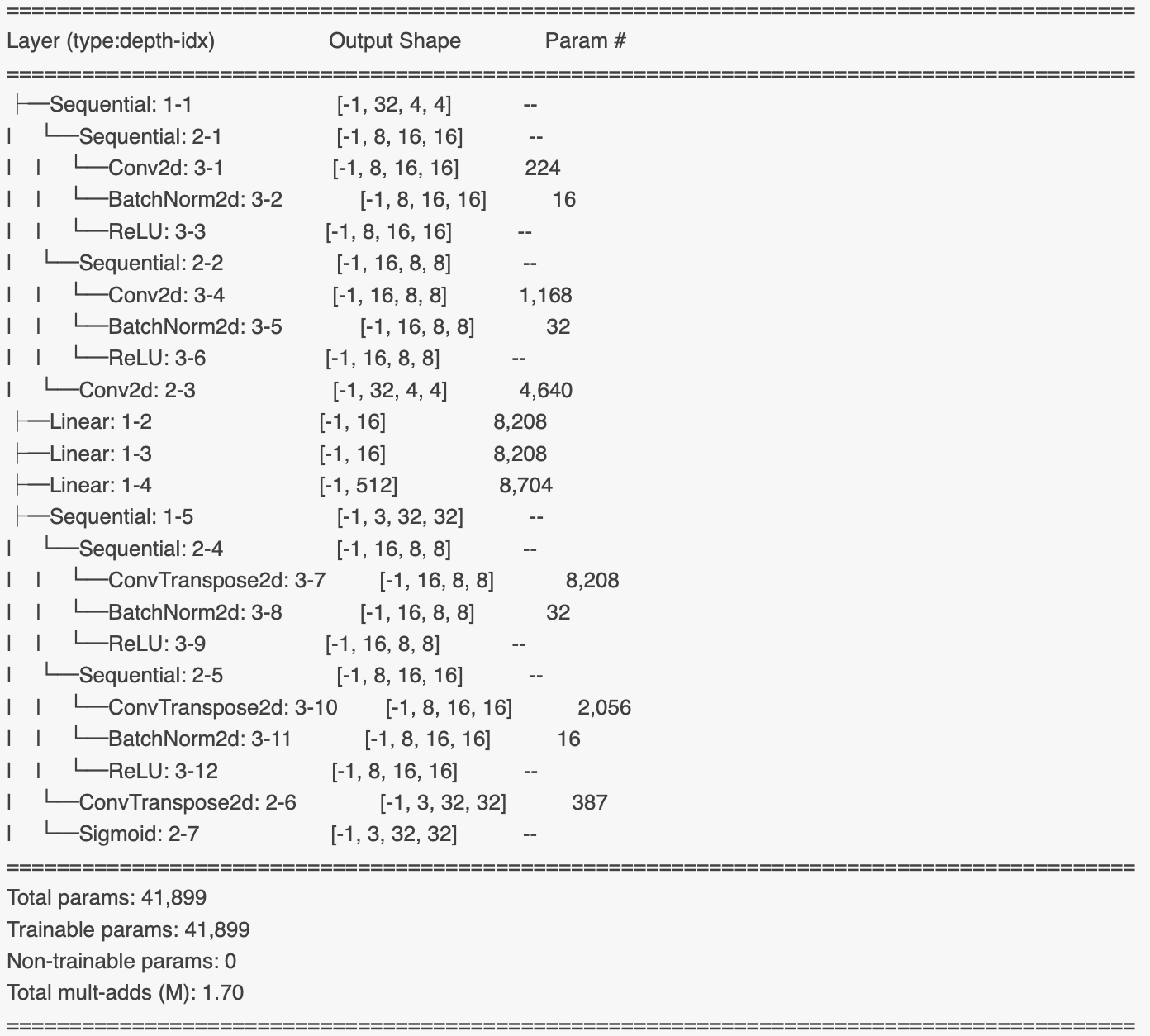
Figure 20. The architecture of convolutional variational autoencoder (VAE)

MNIST dataset contains 70000 handwritten digit images, among which 60000 images are used for training while 10000 are used for testing the model’s generalisation. We use Adam optimiser with learning rate $10^{-3}$, cross-entropy loss as training loss function and train 20 epochs to get the result.

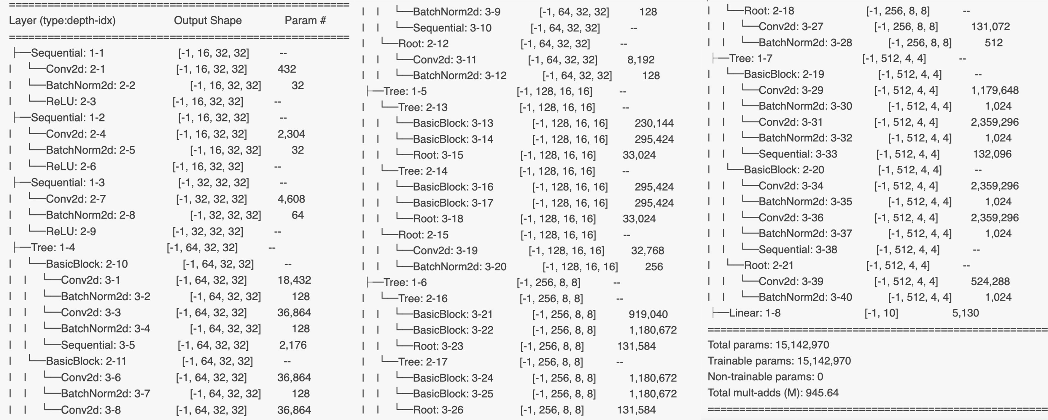
Figure 21. The architecture of Deep Layer Aggregation model trained on CIFAR10 dataset

CIFAR10 dataset contains 60000 32x32 colour images in 10 classes, with 6000 images per class. There are 50000 train images and 10000 test images. We use Stochastic gradient descent (SGD) optimiser with a learning rate of 0.01, momentum 0.9, and weight decay $5\times 10^{-4}$ to train the model with 50 epochs.

We adopt adversarial training to obtain a more robust model for reliability comparison. We use PGD-based adversarial training (Madry et al., 2018) with the same training parameters as normal training to generate attacked data (AEs when successfully attacked) in replacement of all original training data to improve robustness. To be specific, the PGD attack calculates the gradient of training loss with respect to the input. It is deployed with 10 steps and 2/255 step size to generate pixel-level perturbation for training data. The perturbed training data will be utilised over the whole training process.

We use the VAE model to reduce the dimension of data, the architecture of which is shown in Fig. 20. To train the VAE model, we use an Adam optimiser with a learning rate $10^{-3}$ and train 100 epochs.

B.2. Details of the YOLOv3 and VAE Models Trained in the Case Studies

We present more details of the YOLOv3 and VAE models trained in the AUV and UGV case studies, respectively in Table 3 and 4, while in Fig. 22 eight images reconstructed based on the VAE models are shown as examples. For more detailed ML models, datasets and experimental results, please refer to our public repository https://github.com/Solitude-SAMR.

Class	Normal Training		Adversarial Training
	Train	Test	Train	Test
Pipe	0.98343	0.97131	0.92225	0.91380
Floating Ball	0.85765	0.90912	0.83785	0.88291
Gas Canister	0.87230	0.87406	0.83245	0.84319
Gas Tank	0.98930	0.99346	0.93623	0.93769
Oil Barrel	0.84578	0.84258	0.82811	0.82973
Docking Cage	0.88771	0.91076	0.72786	0.71478
mAP	0.90603	0.91688	0.84746	0.85368

(a) AUV

Class	Normal Training		Adversarial Training
	Train	Test	Train	Test
Stop Sign	0.97958	0.99471	0.76873	0.79065
Park Sign	0.98182	0.98158	0.84459	0.82143
Cycle Sign	0.99911	0.98648	0.92750	0.88669
Cross Sign	0.99067	0.98878	0.98850	0.98496
One Way Sign	0.98921	0.99023	0.53972	0.52041
mAP	0.98808	0.98836	0.81381	0.80083

(b) UGV

Table 3. Average Precision (AP) of YOLOv3 for object detection.

VAE model	Train	Test
Recon. Loss	0.002601	0.003048
KL Div. Loss	1.732866	1.729756

(a) AUV

VAE model	Train	Test
Recon. Loss	0.011333	0.016665
KL Div. Loss	4.781964	4.810094

(b) UGV

Table 4. Reconstruction Loss & KL Divergence Loss of VAE model

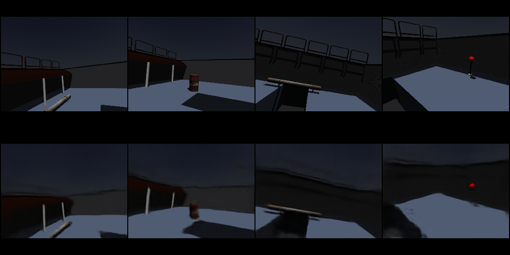
(a) AUV

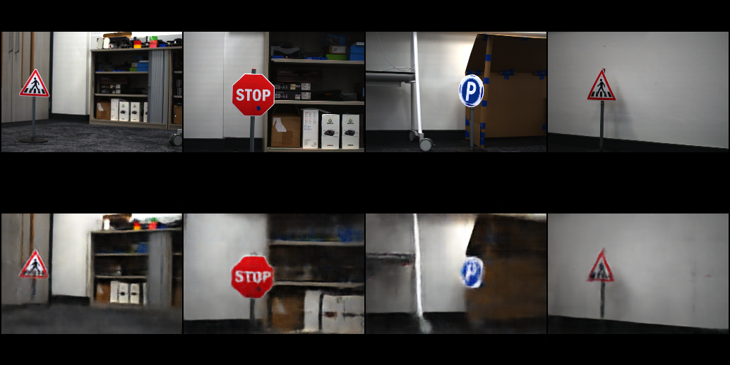
(b) UGV

Figure 22. Original images (top) and corresponding reconstructed images (bottom) by the VAE model.

Appendix C Comparison between RAM and state-of-the-art Robustness Metrics

Table 5. Local robustness evaluation around a selected test seed

	Model	RAM		DeepFool		ERAN (AI2)
		Radius $\epsilon$	$\hat{\lambda}_{i}$	Radius $\epsilon$	Minimal Perturbation	Radius $\epsilon$	Verified Robustness
MNIST	Norm.	0.3	$5.85\times 10^{-19}$	/	0.3151	0.3	0
	Adv.	0.3	$1.93\times 10^{-22}$	/	0.7912	0.3	0
CIFAR-10	Norm.	0.1	$0.4177$	/	0.0189	0.1	0
	Adv.	0.1	$1.92\times 10^{-22}$	/	0.2145	0.1	0

Table 6. Network-wise reliability and robustness evaluation

	Model	RAM			DeepFool
		Radius $\epsilon$	$k$	pmi	Radius $\epsilon$	$k$	Avg. Minimal Perturbation
MNIST	Norm.	0.3	70000	4.74 e-4	/	70000	0.1979
	Adv.	0.3	70000	1.77 e-4	/	70000	0.5141
CIFAR-10	Norm.	0.1	25000	0.3152	/	60000	0.0318
	Adv.	0.1	25000	0.0968	/	60000	0.3368

As shown in Table 5, as before, we study both normally and adversarially trained DL models on the two datasets. In our RAM, the norm ball radius $\epsilon$ is determined by the $r$-separation distance and the local probabilistic robustness evaluation is returned by the estimator (Webb et al., 2019). For a fair comparison, we reuse the same norm ball for applying AI2 which indeed returns the answer “unverified” to the binary question. In contrast, DeepFool aims at finding a minimal perturbation to detect AEs around the same seed. Although DeepFool formulates it as an optimisation problem, its solution has no guarantees to be optimal—the returned solutions are larger than the $r$-separation distance when the AEs are quite rare (the 1st, 2nd and 4th rows). While, at the global level of networks, Table 6 “compares” the reliability metric $pmi$ of our RAM with the averaged minimal perturbation by applying DeepFool. We omit the experiments based on AI2 at such a network-wise level due to the high computational cost of formally verifying all $k$ norm balls. Both the assessments by RAM and DeepFool are reflective of the robustness improvement from a normally trained model to an adversarially trained model. The averaged minimal perturbation derived by DeepFool (or other similar tools concerning worst-case metrics) has limited practical values (Wang et al., 2021; Webb et al., 2019). At the same time, our reliability pmi concerns the overall robustness and generalisability, that predicts the probability of failure for the next input drawn from the OP.

Appendix D Additional Case Study on Healthcare Models

$CORONET$ is a decision-support tool validated in healthcare systems worldwide can aid admission decisions and predict COVID-19 severity in patients with cancer (Lee et al., 2022). The dependability of healthcare AI/ML systems needs to be assured to increase their trustworthiness. In this section, a case of applying our approach on $CORONET$ is studied to validate our reliability assessment methods.

The $CORONET$ model is a decision tree model with 11 dimensions inputs, and three different output labels. Here, we first assess the reliability of a given $CORONET$ model among different $r$-separation radius. The experiment result is shown in Fig. 23(a).

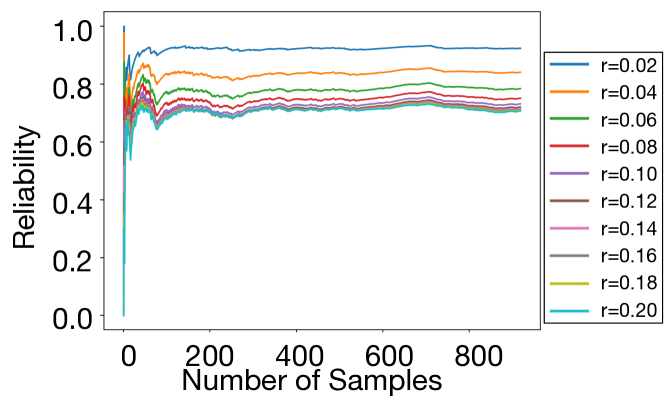
(a) PMI of CORONET dataset with different norm ball radius.

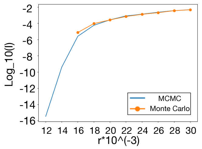
(b) Comparison between the proposed method and Monte-Carlo sampling.

Figure 23. Experiment results of CORONET.

As can be seen from Fig. 23(a), the reliability of the $CORONET$ model decreases as the disturbance radius increases, which is in accordance with our intuition. The higher disturbance would cause more uncertainty.

To further evaluate the effectiveness of our reliability assessment model, we compare our method with naive Monte-Carlo sampling methods. The results are shown in Fig. 23(b).

In this experiment, we collect $10^{5}$ samples based on naive Monte-Carlo sampling method to assess the reliability of the $CORONET$ prediction model. From the experiment results, we can see that the proposed method has an equivalent estimate to the unbiased estimation results of Monte-Carlo sampling. Furthermore, the proposed method can make it much easier to find rare events than the naive Monte Carlo method when the disturbance radius is tiny.

Appendix E Probabilistic Safety Arguments for ML Components

At this lower level of ML components, cf. the SubC7 in Fig. 5, we further decompose and organise our safety arguments in two levels—decomposing sub-functionalities of ML components doing object detection and claiming the reliability of the classification function. In the following sections, we discuss both in details, while focusing more on the latter.

E.1. Arguments for Top Claims on Object Detection at the ML Component-Level

In Fig. 24, we present an argument template, again in the CAE blocks at the ML component-level. It aims at breaking down the claim “The object detection is safe enough” LLC1 to a reliability claim stated in the specified measure. The first argument is over all safety related properties, and presented by a CAE block of substitution. The list of all properties of interest for the given application can be obtained by utilising the Property Based Requirements (PBR) approach (Micouin, 2008), forming the side-claim LLSC1, which is supported by the sub-case SubC10. The PBR analysis, recommended in (Alves et al., 2018) as a method for safety arguments of autonomous systems, is a way to specify requirements as a set of properties of system objects either in a structured language or formal notations. In this work, we focus on the main quantitative property—reliability—while other properties like security and interpretability are omitted and remain an undeveloped sub-case SubC9 in the CAE template.

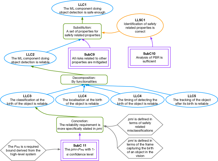
Figure 24. ML component-level arguments breaking down the claim “The object detection component is safe enough” LLC1 to reliability claims of the classification function stated in specific reliability measures SubC11.

Starting from LLC2, we then argue over the decomposition by four sub-functionalities of object detection. At the “birth” of an object in the system’s vision (e.g., the total number of pixels is greater than a threshold), the ML component should accurately classify it, localise it (normally measured by the Intersection over Union (IoU) of bounding boxes) and in good timing (e.g., no later than some frames after its birth). Once initially detected at its birth time, the tracking function on that object should be reliable enough to make decision making by other control components safe. The four sub-functionalities of object detection forms the claims LLC3-LLC5.

To support the reliability of classification at the birth time of the objects LLC3, we concretise the reliability requirements in terms of specific reliability measures, in our case pmi. The “misclassification” and “per input” in pmi need to be clearly defined: (i) we only consider safety-related misclassification events; (ii) an input refers to the image frame capturing the “birth” of an object in the camera’s vision (so that images can be treated as independent conforming to the definition of pmi). We are then interested in the claim of a bound on pmi with $(1-\alpha)$ confidence, where $P_{req}$ is a required bound derived from higher level safety analysis.

While the reliability of the other three sub-functionalities can be similarly concretised by some quantitative measures, e.g. IoU for localisation, they remain undeveloped in this article and form important future work.

E.2. Low-Level Arguments for Classification Based on the RAM

In this section, we present SubC11 and show how to support a reliability claim stated in pmi based on our RAM developed in Section 5—the “backbone” of the probabilistic arguments at this lower level. Essentially, we argue over the four main steps of our RAM as shown in Fig. 25. Note that, depending on the data dimensionality of the specific application, we may either use the “low-dimensional” version of our RAM, where the whole input space is partitioned into cells, or apply the “high-dimensional” version, in which norm balls (of relatively spare data) are determined instead (cf. Remark 4) based on the collected data to form the sample frame (representing the population of all norm balls partitioning the whole input space). Indeed, the method of exhaustively partitioning cells is also applicable to high-dimensional data, but it would yield an extremely large number of cells that is not only infeasible to examine exhaustively but also quite difficult to index for sampling. That said, for high-dimensional datasets, we determine norm balls from the data instead, forming a smaller and more practical sampling frame. However, the price paid is at introducing two more noise factors in the assurance—the bias/error from the construction of the sampling frame and the relatively low sample rate. The former can be mitigated by conventional ways of checking (and rebuilding if necessary) the sampling frame, while the latter has been captured and quantified by the variance of the point estimate (cf. Eqn. (15) and Assumption 7).

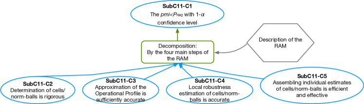
Figure 25. Arguments over the four main steps in the proposed RAM.

Figures 26 to 29 show the arguments based on steps 1 to 4 of our RAM, respectively. While the arguments presented in CAE are self-explanatory together with the technical details articulated in Section 5, we note that i) all modelling assumptions are presented as side-claims of arguments that need more application-specific development and justification; and ii) the development of some claims is omitted for brevity, because they are generic claims and thus can be referred to other works, e.g. (Ashmore et al., 2021), for SubC11-C3.2 and SubC11-C3.3 when we treat the OP estimator as a common data-driven learning model.

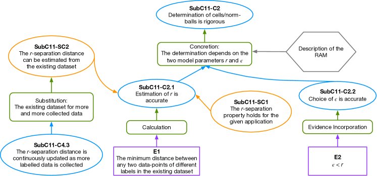
Figure 26. Arguments based on the step 1 of the RAM.

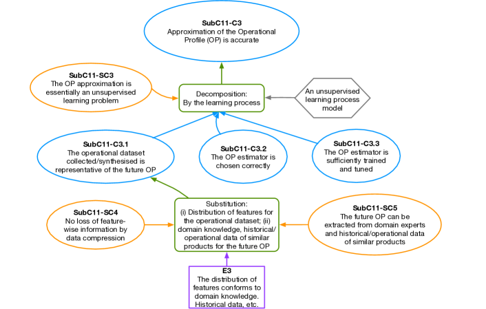
Figure 27. Arguments based on the step 2 of the RAM.

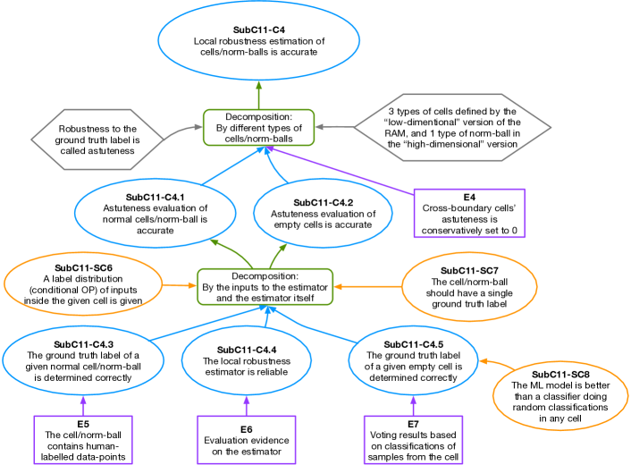
Figure 28. Arguments based on the step 3 of the RAM.

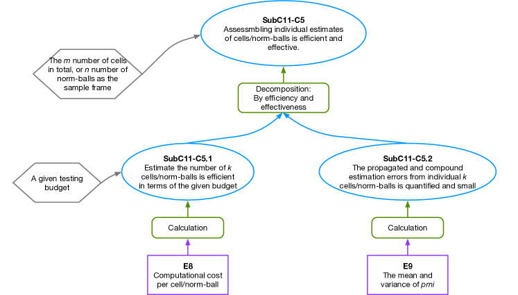
Figure 29. Arguments based on the step 4 of the RAM.