The Norm Must Go On: Dynamic Unsupervised Domain Adaptation by Normalization

Abstract

Domain adaptation is crucial to adapt a learned model to new scenarios, such as domain shifts or changing data distributions. Current approaches usually require a large amount of labeled or unlabeled data from the shifted domain. This can be a hurdle in fields which require continuous dynamic adaptation or suffer from scarcity of data, e.g. autonomous driving in challenging weather conditions. To address this problem of continuous adaptation to distribution shifts, we propose Dynamic Unsupervised Adaptation (DUA). By continuously adapting the statistics of the batch normalization layers we modify the feature representations of the model. We show that by sequentially adapting a model with only a fraction of unlabeled data, a strong performance gain can be achieved. With even less than 1% of unlabeled data from the target domain, DUA already achieves competitive results to strong baselines. In addition, the computational overhead is minimal in contrast to previous approaches. Our approach is simple, yet effective and can be applied to any architecture which uses batch normalization. We show the utility of DUA by evaluating it on a variety of domain adaptation datasets and tasks including object recognition, digit recognition and object detection.

1 Introduction

Present day Deep Neural Networks (DNNs) show promising results when both training and testing data belong to the same distribution [26, 16, 69]. However, if there is a domain shift, i.e. when the testing data comes from a different domain, neural networks struggle to generalize [38, 4, 10]. In fact, even if there is only a slight distribution shift, the performance of neural networks is reported to already degrade significantly [18, 48].

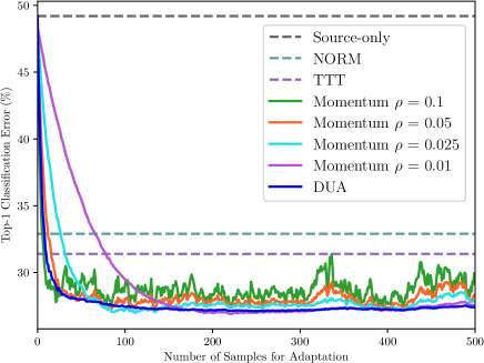
(a) CIFAR-10C results.

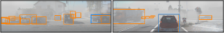
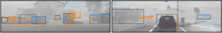
(b) Detections in foggy weather without (top) and with (bottom) DUA. We overlay the detection results (blue) and the ground truth (orange).

Figure 1: Exemplary DUA results. a) Mean classification error over 15 different corruption types (at the most severe level 5) on CIFAR-10C [18]. We outperform the state-of-the-art NORM [55, 42] and TTT [61], while using less than 1% of unlabeled data from the corrupted test set only. Our proposed adaptive momentum scheme leads to both fast and stable improvements in contrast to fixing the momentum parameter $\rho$. b) Qualitative results for object detection in degrading weather conditions: our DUA (bottom) significantly improves the performance of a KITTI [11] pre-trained YOLOv3 [49] on KITTI-Fog [14]. Best viewed in color.

One way to overcome the performance drop during domain shifts is to obtain labeled data from the shifted domain and re-train the network. However, manual labeling of large amounts of data imposes significant human and monetary costs. These issues are addressed by Unsupervised Domain Adaptation (UDA) approaches, e.g. [4, 12, 10, 33, 68, 77, 17, 53, 24, 34]. For UDA, the goal is to modify the network parameters in such a way that it can adapt in an unsupervised manner to out-of-distribution testing data. Traditionally, these approaches require labeled training data along with a large amount of unlabeled testing data.

In many practical scenarios, the traditional requirements, i.e. access to both labeled training and large amounts of unlabeled testing data can often not be fulfilled. For example, in the medical domain, pre-trained models are often provided without access to the training data (which is kept private due to privacy regulations). Likewise, some application domains benefit from dynamic adaptation to a changing environment. For example, consider object detectors for autonomous vehicles, which are usually trained on mostly clear weather images, e.g. [11, 15, 59]. In real-world scenarios, however, weather can suddenly deteriorate, resulting in significant performance degradation [41, 40]. In such cases, it is not feasible to obtain labeled training data captured in degrading weather and re-train the detector from scratch. A better solution is to dynamically adapt the detector, given only a few (unlabeled) bad weather examples.

In this work, we show that one hindrance in domain generalization is the statistical difference in mean and variance between train and (shifted) test data. Thus, during inference, we adapt the running mean and variance which are calculated during training by the batch normalization layer [21]. Moreover, we adapt the statistics dynamically in an online manner on a tiny fraction of test data. For adaptation, we form a small batch by augmenting each incoming sample. In order to ensure stable adaptation and fast convergence we propose an adaptive update schema.

Related approaches [28, 55, 42, 64] typically ignore the training statistics and recalculate the batch statistics from scratch for the test data. This, however, requires large batches of test data. We argue that a large batch of test data might not always be available in real-world applications, e.g. autonomous cars adapting to challenging weather (see Figure 1). We show that a strong performance gain can be achieved by adapting the running mean and variance in an online manner (one sample at a time). In particular, we require only a small number of sequential samples from the out-of-distribution data.

Our contributions can be summarized as follows:

• We show that online adaptation of batch normalization parameters on a tiny fraction of unlabeled out-of-distribution test data can provide a strong performance gain. With even less than 1% of unlabeled test data, DUA already performs competitively to strong baselines which use the entire test set for adaptation.

• DUA is simple, unsupervised, dynamic and requires no back propagation [51] to work. Since the computational overhead is also negligible, it is perfectly suited for real-time applications.

• We evaluate DUA on a variety of domain shift benchmarks, demonstrating its strong performance. We achieve state-of-the-art results on most benchmarks while being competitive on the remaining.

• We show that our dynamic adaptation method works on a variety of different tasks and different architectures. To the best of our knowledge, we are the first to show dynamic adaptation for object detection.

2 Related Work

Unsupervised Domain Adaptation (UDA) has received a significant amount of interest recently. We summarize these approaches in four categories: minimizing discrepancy between domains, adversarial approaches, self-supervised approaches and correcting domain statistics.

Discrepancy reduction between source and target domains is usually performed at specific network layers or in a contrastive manner. Long et al. [37] match the mean embeddings from task specific layers. Sun et al. [57, 58] minimize the second order statistics to align the source and target domains. They apply a linear transformation on the source domain to align it with the target domain. Zellinger et al. [75] propose to match higher order moments by introducing a Central Moment Discrepancy (CMD) metric to learn domain invariant features. Chen et al. [2] propose to match third and fourth order statistics of the source and target domains for unsupervised domain adaptation. On the other hand, [65, 23] use contrastive learning [6] to reduce discrepancy between domains.

Adversarial discriminative approaches align the features from the source and target domains mostly by using the domain confusion loss. Ganin et al. [10] propose a method which is based on the philosophy that predictions must be made on features which are non-discriminative during training. A novel gradient reversal layer is proposed which brings the features from the source and target domains closer by maximizing the domain confusion loss. Tzeng et al. [63] also rely on maximizing the domain confusion loss for unsupervised domain adaptation. Hong et al. [19] use a fully convolutional network and use generative adversarial networks [13] to address the problem of synthetic-to-real feature alignment. Chen et al. [5] align the global and class wise features by using a generative adversarial network. Similar approaches for UDA have also been followed for a variety of tasks, including object detection [17, 4, 24, 66, 68, 70, 71, 77, 8], object classification [33, 34, 36, 47, 30] and semantic segmentation [22, 3, 78, 1, 72, 29] for both 2D and 3D data.

Self Supervision has also been used for the purpose of unsupervised domain adaptation. Sun et al. [60] combine different self supervised auxiliary tasks for domain adaptation. Sun et al. [61] also propose Test Time Training (TTT) with self supervision. They put forward the idea of removing the self-imposed condition of a fixed decision boundary at test time. In their work they use the rotation prediction task [12] as a self supervised task in order to adapt the network to out-of-distribution test data.

Correcting the domain statistics calculated by the batch normalization layer [21] has also been used for UDA. Li et al. [28] propose Adaptive Batch Normalization where they show that recalculating the batch normalization parameters from scratch for the test set can improve generalization of DNNs. Carlucci et al. [39] propose domain adaptation layers which can learn a hyperparameter during training to find the optimal mixing of statistics from the source and target domain. Singh et al. [56] study the effect of lower batch sizes during training and show that DNNs using batch normalization layers are effected by lower batch sizes. They propose an auxiliary loss for remedy. Similarly, [42, 55, 76] also show that recalculation of batch normalization statistics from scratch for test data can be helpful to address the problem of distribution shift between source and target domains. Wang et al. [64] also recalculate the batch normalization statistics for the test data. Further, they calculate the loss from the entropy of predictions and adapt the scale and shift parameters of batch normalization layers. It is important to point out that [28, 42, 55, 64] share the same philosophy of a variable decision boundary at test time as TTT [61].

Our work closely resonates with [28, 42, 55, 64] and is also similar in philosophy to TTT [61], aiming for a variable decision boundary at test time. However, we differ from them in several fundamental ways: In [28, 42, 55, 64], the training statistics are ignored and the batch statistics are recalculated from the test set. For this reason they require large batches from the test set. However, in general, large batches of test data might not be available. Instead, we adapt the statistics calculated from the training data in an online manner (on each incoming sample). We show competitive results by using less than 1% of unlabeled test data in contrast to all previous approaches which use the complete test set. Further, contrary to previous approaches, such as [64, 61], our method does not require back propagation. Our scenario is more realistic for dynamic adaptation where we can obtain only a single test frame at one time.

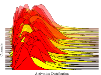
(a) Source Model

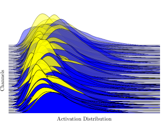
(b) Model Adapted with DUA

Figure 2: Density plots of output distribution for the 64 channels of the last batch normalization layer of ResNet-26 trained on CIFAR-10. a) Yellow is the output distribution of the training data. Red is the output distribution of the shifted test data, i.e. corrupted with Contrast Level-5 [18]. The misalignment of the feature responses is one reason for the performance drop. b) Yellow is the output distribution of the training data. Blue is the output distribution of the shifted test data, i.e. corrupted with Contrast Level-5, after adaptation with DUA. DUA aligns the output distribution from corrupted data closely with the clean (training) distribution. Best viewed in color.

3 Approach

We first summarize batch normalization [21] in Section 3.1 as it lies at the center of our approach. Section 3.2 then details our DUA approach.

3.1 Batch Normalization

Ioffe and Szegedy [21] proposed a batch normalization layer which has become an important component of modern day DNNs. Each batch normalization layer in the network calculates the mean and variance for each activation coming from the training data $X$, and normalizes each incoming sample $x$ as

$$\hat{x}=\frac{x-{\operatorname{\mathbb{E}}\!\left[{X}\right]}}{\sqrt{{\operatorname{Var}\!\left[{X}\right]}+\epsilon}}\cdot\gamma+\beta,$$ (1)

where $\gamma$ and $\beta$ are the scale and shift parameters, and $\epsilon$ is used for numerical stability. The expected value $\operatorname{\mathbb{E}}\!\left[{X}\right]$ of the training statistics is estimated through the running mean,

$${\hat{\mu}_{k}}=(1-\rho)\cdot{\hat{\mu}_{k-1}}+\rho\cdot{\mu_{k}},$$ (2)

and the variance of the training statistics $\operatorname{Var}\!\left[{X}\right]$ is estimated through running variance,

$${\hat{\sigma}_{k}^{2}}=(1-\rho)\cdot{\hat{\sigma}_{k-1}^{2}}+\rho\cdot\sigma_{k}^{2}.$$ (3)

Here, $\hat{\mu}$ and $\hat{\sigma}^{2}$ are the estimated mean and variance from the training data, whereas $\mu$ and $\sigma^{2}$ represent the mean and variance of the incoming batch. The hyperparameter $\rho$ is the momentum term (default $\rho=0.1$) and $k$ denotes each training step. Intuitively, $\rho$ can be thought of as the factor which controls how much the existing estimate of statistics is affected by the statistics of the incoming batch. A larger momentum value would essentially give more weight to the calculated statistics of the incoming batch. Empirically, it has been shown that batch normalization helps to train faster and also stabilize the training process[54].

The behavior of batch normalization differs during training and testing as follows:

Training:

During training, the batch normalization layer calculates the running mean and variance over the complete training set. The scale parameter $\gamma$ and shift parameter $\beta$ from Eq. (1) are learned by back propagation. Running mean and variance is updated during each forward pass with the new batch statistics.

Testing:

During inference, the running mean and variance of the batch normalization layer is fixed. Each new sample encountered during testing is normalized by using the population statistics calculated during training.

3.2 Dynamic Unsupervised Adaptation

Let $\Phi_{\text{src}}$ be the network trained solely with source data $X_{\text{src}}$. Our goal is to adapt the trained model to out-of-distribution target data $X_{\text{tar}}$ in an unsupervised manner. The batch normalization layer performs consistently well when train and test data belong to a similar distribution [16, 69]. However, in many practical scenarios this is not the case. It has been shown that when out-of-distribution test data is encountered, batch normalization can hamper the performance significantly [28, 42, 55, 64, 67, 9]. One reason for the performance degradation is the misalignment of the activation distribution between training and out-of-distribution test data as shown in Figure 2(a). Thus, our adaptation process aligns the activation distribution between training and shifted test data as depicted in Figure 2(b).

In our proposed adaptation schema, all the parameters of the network $\Phi_{\text{src}}$, other than the running mean and running variance are fixed. We only adapt the $\operatorname{\mathbb{E}}\!\left[{X}\right]$ and $\operatorname{Var}\!\left[{X}\right]$ from Eq. (1) to the new statistics of $X_{\text{tar}}$, by using the training statistics obtained from $X_{\text{src}}$ as a prior. The training statistics are updated by using one image after the other, i.e. processing new examples of the (shifted) test data in a sequential manner as they arrive. The naïve approach would be to update the statistics by using Eqs. (2) and (3) with a fixed momentum parameter $\rho$. However, as shown in Figure 1(a), such fixed momentum leads to a couple of problems: The adaptation performance is either unstable or converges rather slowly. This is because with the default parameters the adaptation of the running mean and variance is highly unstable, as shown in Figure 3(a). Thus, for stable and fast convergence we adapt the momentum with each incoming sample. More formally, we update the mean and variance consecutively:

$${\hat{\mu}_{k}}=(1-(\rho_{k}+\zeta))\cdot{\hat{\mu}_{k-1}}+(\rho_{k}+\zeta)\cdot\mu_{k},$$ (4)

with

$${\hat{\mu}_{0}}={\hat{\mu}_{s}},\quad\rho_{k}=\rho_{k-1}\cdot\omega,\quad\rho_{0}=0.1,$$ (5)

and

$${\hat{\sigma}^{2}_{k}}=(1-(\rho_{k}+\zeta))\cdot{\hat{\sigma}^{2}_{k-1}}+(\rho_{k}+\zeta)\cdot\sigma^{2}_{k},$$ (6)

with

$${\hat{\sigma}^{2}_{0}}={\hat{\sigma}^{2}_{s}},\quad\rho_{k}=\rho_{k-1}\cdot\omega,\quad\rho_{0}=0.1.$$ (7)

Here, $\omega$ $\in$ $(0,1)$, is the momentum decay parameter, whereas $\zeta$, with $0\,$<$\,\zeta\,$<$\,\rho_{0}$, is a constant and defines the lower bound of the momentum. As the momentum $\rho_{k}$ decays, the later samples will have a smaller impact. Our adaptive momentum scheme has a direct impact on how the running mean and variance are adapted. The adaptation becomes stable as compared to default parameters, which is visible in Figure 3(b).

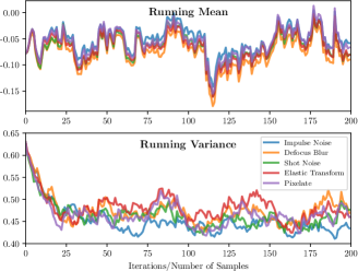
(a) Default Parameters

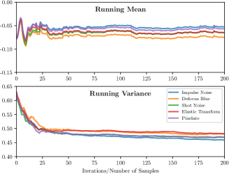
(b) DUA

Figure 3: Running mean and variance of a single channel from the last batch normalization layer for different corruptions in CIFAR-10C. a) Running mean and variance values at each adaptation iteration when default momentum parameters are used. The values are highly unstable which leads to unstable adaptation. b) DUA proposes to use an adaptive momentum schema which leads to fast and stable convergence. This is because of the stability of the running mean and variance values. Initially, the distributions are far apart and thus, we want larger update steps (faster assimilation), whereas later on smaller update steps are beneficial.

Whenever we obtain a new sample from the (shifted) test distribution, we make a small batch by augmenting the incoming sample. In particular, we use random horizontal flipping, random cropping and rotation. We take care that the augmentations we use do not correlate with the shifted test data in our experiments (e.g. we do not augment with any of the corruptions in CIFAR-10/100C [18]). An example of a batch we use for adaptation is provided in the supplemental material. Throughout our evaluations, we found that making a small batch from a single image stabilizes the adaptation process and improves the results, although this is not strictly necessary for our adaptation scheme to work. The effect of batches and augmentations is analyzed in our ablation study in Sec. 5.

	gaus	shot	impul	defcs	gls	mtn	zm	snw	frst	fg	brt	cnt	els	px	jpg	mean
Source	67.7	63.1	69.9	55.3	56.6	42.2	50.1	31.6	46.3	39.1	17.1	74.6	34.2	57.9	31.7	49.2
TTT	45.6	41.8	50.0	21.8	46.1	23.0	23.9	29.9	30.0	25.1	12.2	23.9	22.6	47.2	27.2	31.4
NORM	44.6	43.7	49.1	29.4	45.2	26.2	26.9	25.8	27.9	23.8	18.3	34.3	29.3	37.0	32.5	32.9
DUA	34.9	32.6	42.2	18.7	40.2	24.0	18.4	23.9	24.0	20.9	12.3	27.1	27.2	26.2	28.7	26.8
Source	28.8	22.9	26.2	09.5	20.6	10.6	09.3	14.2	15.3	17.5	07.6	20.9	14.7	41.3	14.7	18.3
TENT	15.8	13.5	18.7	08.1	18.7	09.1	08.0	10.3	10.8	11.7	06.7	11.6	14.1	11.7	15.2	12.3
DUA	15.4	13.4	17.3	08.0	18.0	09.1	07.7	10.8	10.8	12.1	06.6	10.9	13.6	13.0	14.3	12.1

Table 1: Top-1 Classification Error (%) for each corruption in CIFAR-10C at the highest severity (Level 5). Source shows the results from the same model trained on the clean train set and tested on the corrupted test set. For a fair comparison with TTT and NORM, we use ResNet-26 (top), while for TENT, we use the WRN-40-2 (bottom) from their official implementation. Smallest error is shown in bold.

	gaus	shot	impul	defcs	gls	mtn	zm	snw	frst	fg	brt	cnt	els	px	jpg	mean
Source	89.5	88.8	95.5	68.4	83.3	65.0	63.5	62.4	74.9	70.3	42.9	83.0	61.1	84.4	65.5	73.2
TTT	83.8	83.0	86.8	59.9	77.7	57.9	59.2	61.5	70.6	70.5	44.5	69.8	56.5	80.2	60.3	68.1
NORM	72.5	72.7	77.1	48.6	69.3	49.7	47.9	59.5	59.7	58.4	41.8	53.1	58.8	57.3	67.7	59.6
DUA	67.9	67.3	72.6	47.9	66.1	51.6	46.6	58.1	57.6	54.4	41.3	58.6	55.3	53.3	60.7	57.3
Source	65.7	60.1	59.1	32.0	51.0	33.6	32.4	41.4	45.2	51.4	31.6	55.5	40.3	59.7	42.4	46.7
TENT	40.3	39.9	41.8	29.8	42.3	31.0	30.0	34.5	35.2	39.5	28.0	33.9	38.4	33.4	41.4	36.0
DUA	42.2	40.9	41.0	30.5	44.8	32.2	29.9	38.9	37.2	43.6	29.5	39.2	39.0	35.3	41.2	37.6

Table 2: Top-1 Classification Error (%) for each corruption in CIFAR-100C at the highest severity (Level 5).

	gaus	shot	impul	defcs	gls	mtn	zm	snw	frst	fg	brt	cnt	els	px	jpg	mean
Source	98.4	97.7	98.4	90.6	93.4	89.8	81.8	89.5	85.0	86.3	51.1	97.2	85.3	76.9	71.7	86.2
TTT	96.9	95.5	96.5	89.9	93.2	86.5	81.5	82.9	82.1	80.0	53.0	85.6	79.1	77.2	74.7	83.6
NORM	87.1	89.6	90.5	87.6	89.4	80.0	71.9	70.6	81.5	66.9	47.8	89.8	73.5	64.2	68.5	77.3
DUA	89.4	87.6	88.1	88.0	88.6	84.7	74.3	77.8	78.4	68.6	45.6	95.9	72.2	66.5	67.4	78.2

Table 3: Top-1 Classification Error (%) for each corruption in ImageNet-C at the highest severity (Level 5). Source refers to results obtained from a model pre-trained on the original ImageNet and tested on the corrupted test sets. All results are obtained using a ResNet-18 backbone. Smallest error is shown in bold.

4 Results

In the following, we evaluate DUA on a variety of tasks and benchmarks. First, we summarize the datasets. Next, we introduce the approaches to which we compare. Lastly, we present our detailed results.

4.1 Benchmarks and Tasks

CIFAR-10/100C:

CIFAR-10C and CIFAR-100C [18] are image classification benchmarks to test a model’s robustness w.r.t. covariate shifts. These benchmarks add different corruptions to the original test set of CIFAR-10/100 [25] at 5 severity levels. Following the common protocol [64, 42, 61], we evaluate on 15 types of corruptions.

ImageNet-C:

Similar to the CIFAR-10/100C benchmarks, ImageNet-C [18] is also an image classification dataset introducing different corruptions at several severity levels to the original test set of ImageNet [7].

KITTI:

To test DUA’s adaptation capabilities on the task of object detection for autonomous vehicles we use the well-known KITTI [11] dataset. Further, we also use the KITTI-Rain and KITTI-Fog datasets [14] to test the adaptation performance of a KITTI pre-trained model in degrading weather.

4.2 Baselines

We compare our DUA against the following approaches:

• Source: denotes the results of the corresponding baseline model trained only on source data, i.e. without any adaptation to the test data.

• TTT: Test Time Training (TTT) [61] adapts the network parameters by using an auxiliary task on each (out-of-distribution) data sample before testing it.

• NORM [55, 42]: ignores the train statistics completely and recalculates the batch normalization statistics on the entire test set, leveraging larger batch sizes.

• TENT: Test time entropy minimization (TENT) [64] recalculates the batch normalization statistics and additionally modifies the scale and shift parameters ($\gamma$ and $\beta$) of the batch normalization layers through back propagation. They obtain the gradients by calculating the prediction entropy on large batches from the out-of-distribution test data.

4.3 Experiments

In this section, we provide a description of all the results obtained on different datasets and benchmarks. We test our DUA during slight distribution shifts and severe domain shifts as well. For our results we always use less than 1% of unlabeled test data and adapt on each incoming sample in a sequential manner (the exact numbers of test samples used for adaptation in our experiments are listed in the supplemental material). Results for all other baselines have been obtained by adapting on the complete test set as stated in their original papers. Note, we also do not need to control for shuffling of the test set in contrast to other approaches [64, 55, 42]. For adaptation, unless stated otherwise, we fix the momentum decay parameter $\omega=0.94$, and the lower bound $\zeta=0.005$. Further details for all the experiments are provided in the supplemental material. For reproducibility, code for DUA is available at this repository: https://github.com/jmiemirza/DUA

CIFAR-10/100C

	Car	Pedestrian	Cyclist
Source only	30.9	34.1	16.2
DUA	51.4	48.5	33.1
Fully Supervised	71.3	64.5	63.2

(a)

	Car	Pedestrian	Cyclist
Source only	80.7	66.7	54.6
DUA	86.3	70.3	66.7
Fully Supervised	92.3	76.1	78.2

(b)

Table 4: Results for KITTI pre-trained YOLOv3 tested on rain and fog datasets. We report the Mean Average Precision (mAP@50). a) Results for the most severe fog level, i.e. $30$m visibility. b) Results for the most severe rain level, i.e. $200$mm/hr rain intensity.

For a fair comparison to TTT and NORM we use ResNet-26 [16] and follow the parametrization in their official implementations${}^{\text{,}}$. Similarly, for TENT we use the Wide-ResNet-40-2 [73] from their official implementation.

Table 1 shows the results for the highest severity level on CIFAR-10C. Note that we achieve a new state-of-the-art. All other approaches use the complete test set and most also use larger batch sizes and control shuffling of test data. Results on CIFAR-100C are listed in Table 2. Here, DUA outperforms TTT and NORM while being competitive with TENT. Results for lower severity levels are provided in the supplemental material, demonstrating that DUA provides strong results for less severe corruptions as well.

ImageNet-C

For evaluations on ImageNet-C we take an off-the-shelf pre-trained ResNet-18 from PyTorch [44]. Table 3 shows the top-1 error for the highest severity level. DUA performs on-par with all the baselines for ImageNet-C. Results for lower severity levels are provided in the supplemental.

Object Detection

We also test our approach for object detection and show considerable improvement. We conduct these experiments with YOLOv3 [49]. However, our approach could also be applied to other base architectures such as [50, 31, 35, 62], which use batch normalization.

For evaluating our approach on object detection we consider the two following scenarios:

• Evaluation during covariate shifts; These evaluations are performed to adapt to rain and fog conditions.

• Evaluation during domain shifts; These evaluations test for domain adaptation between datasets.

In degrading weather, a sharp drop in performance of present day object detectors has been noted [41, 40]. Our goal is to dynamically adapt a detector trained on clear weather data to degrading weather conditions.

Adaptation results for the most severe forms of fog and rain augmented on KITTI are shown in Table LABEL:tab:kitti_fog_rain:fog and LABEL:tab:kitti_fog_rain:rain, respectively. For fog, the mean improvement across all commonly evaluated classes (i.e. car, pedestrian and cyclist) over the source model is 17.7% mAP. Similarly, we also achieve notable improvements while adapting to rain. Here, the mean improvement over the source model is 7.1% mAP. Additional results for varying severity of fog and rain are provided in the supplemental material.

Additional Results

We also demonstrate the benefits of DUA on several other datasets and adaptation tasks in the supplemental material. In particular, we evaluate DUA on:

Digit Recognition:

DUA can successfully be used for domain adaptation across datasets which we demonstrate for the task of digit recognition. In particular, we use MNIST [27] and USPS [20], which are datasets consisting of handwritten digits. Additionally, we use SVHN [43], a dataset containing house numbers obtained from Google street view images.

Office-31

[52]:    is a visual domain adaptation dataset for object classification, containing 31 categories of common objects found in an office environment, captured in three different settings. These include images captured by Webcam, DSLR and gathered from Amazon. We test for domain adaptation across all three settings.

VIS-DA:

The Visual Domain Adaptation [45] dataset (VIS-DA) is a large scale image recognition dataset which contains 12 classes. The training set consists of synthetically rendered images. The test set consists of real images cropped from the MS-COCO dataset [32].

SODA10M:

The large scale object detection dataset for autonomous vehicles SODA10M [15] provides data captured during day and night. We test for adaptation from day to night. Further, we test for domain adaptation between KITTI and SODA10M.

5 Ablation Studies

In this section we present detailed ablation studies in order to examine our approach more closely.

5.1 Sample Order Does Not Matter

To understand if the ordering of the incoming samples for adaptation holds any significance, we run DUA for 300 independent runs (on CIFAR-10C) and randomly shuffle the test set in each run. The initial, source-only, mean error is $49.2\,\%$. The largest standard deviation over the 300 runs occurs after adaptation on 5 samples, where we achieve $36.4\pm 0.4$. Already after 25 samples, we achieve $28.3\pm 0.19$. The performance saturates after 100 samples and we achieve $27.2\pm 0.09$ (a detailed plot is provided in supplemental material). Thus, the performance of DUA is stable across all independent runs with very little deviation. These results are important to understand that DUA can be used with any arrangement of incoming data.

5.2 Continuous Dynamic Adaptation

In order to understand how good can DUA handle the real-life scenarios where different weather conditions can occur interchangeably, we test DUA for such a scenario on KITTI-Fog: day$\to$fog$\to$day$\to$etc. Results are shown in Fig. 4. Note the only minor drop on the source domain (e.g. 5.8% worse than the day baseline at iteration 100) and that we can quickly recover the same performance again. This shows that despite not being an incremental learning approach, DUA still remembers information from the previous domain. We conjecture that this is because learned weights are not changed during adaptation. DUA only shifts the activation distributions at test time.

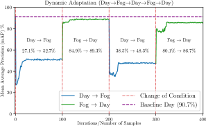
Figure 4: Dynamic adaptation scenario for DUA. We let a KITTI-pretrained model adapt to fog and then back to the original KITTI dataset for two cycles in order to show how well DUA can dynamically adapt to changing weather conditions.

5.3 Ablating Batch Normalization Layers

We investigate the effect of adapting only selected batch normalization layers in Figure 5. For this, we adapt batch normalization layers of specific ResNet-26 blocks while keeping all others fixed. As can be seen from the plot, the best performance is obtained by adapting all batch normalization layers in the architecture. Individual improvements are slightly larger at later batch normalization layers.

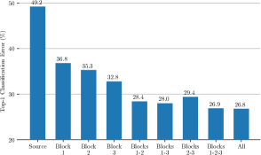
Figure 5: Results on CIFAR-10C after adapting the batch normalization layers of specific ResNet-26 blocks. ‘All’ refers to adapting all batch normalization layers. This includes the last batch normalization layer after the three ResNet blocks.

5.4 Effect of Augmentation

As explained in Section 3.2, we form a small batch of augmented versions from each incoming sample. In Figure 6, we ablate different augmentations and batch sizes to study their effects. Apart from providing stability to our adaptation procedure, making a small batch and augmenting it randomly also provides further improvements. For our experiments, we form a batch of size 64 from each incoming image by augmenting it. However, even a batch size of only 8 suffices to benefit from DUA (with only minor sacrifice in performance).

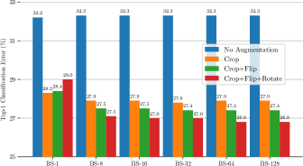
Figure 6: Effects of different batch sizes and augmentations on CIFAR-10C with ResNet-26. DUA makes a batch out of each sequential image by using different random augmentations. Note that the source-only error (without adaptation) is 49.2%.

6 Conclusion

We have shown that even slight distribution shifts between train and test data can greatly hamper the performance of present day neural networks. We address this limitation by our DUA, which adapts the statistics of a trained model in a sequential manner on each unlabeled sample coming from out-of-distribution test data. To ensure fast and stable adaptation, we introduce an adaptive momentum scheme. DUA does not require access to training data but only needs a fraction of test data to achieve competitive results to strong baselines. Extensive experimentation on a variety of challenging benchmarks and tasks demonstrate the utility of our method on a broad range of batch normalization-based architectures. Since we can dynamically adapt to shifting distributions at a minimal computational overhead, DUA is also well-suited for both real-time systems and embedded devices.

Acknowledgments

We gratefully acknowledge the financial support by the Austrian Federal Ministry for Digital and Economic Affairs, the National Foundation for Research, Technology and Development and the Christian Doppler Research Association. This work was also partially funded by the Austrian Research Promotion Agency (FFG) under the project High-Scene (884306).

In the following, we summarize our evaluation details to support reproducibility (Section A) and provide additional detailed results (Section B).

Appendix A Evaluation Details

Number of Samples:

DUA requires only a tiny fraction of the (unlabeled) test set to achieve competitively strong results. The exact numbers are listed in Table 5. Note that after adaptation on these specific number of samples, the adaptation performance always saturates. We conducted all experiments on a single NVIDIA^® GeForce^® RTX 3090.

Dataset	Total no. of samples in	No. of samples used	% of samples used
	test set	for adaptation	for adaptation
CIFAR-10C [18]	10000	080	0.8%
CIFAR-100C [18]	10000	080	0.8%
ImageNet-C [18]	50000	100	0.2%
MNIST [27]	10000	030	0.3%
SVHN [43]	26032	030	0.1%
USPS [20]	02007	020	0.9%
Office-31 [52]	04110	040	0.9%
VIS-DA [45]	05534	040	0.7%
KITTI [11]	03741	025	0.6%
KITTI-Rain [14]	03741	025	0.6%
KITTI-Fog [14]	03741	025	0.6%
SODA-10M [15]	04991	030	0.6%
SODA10M-Day [15]	03347	030	0.8%
SODA10M-Night [15]	01644	015	0.9%

Table 5: Available number of samples in the test sets vs. number of samples used for adaptation. Note that all datasets except for KITTI have dedicated test sets. On KITTI, we divide the training set of 7481 images into 3740 train and 3741 test images.

Batch Augmentations:

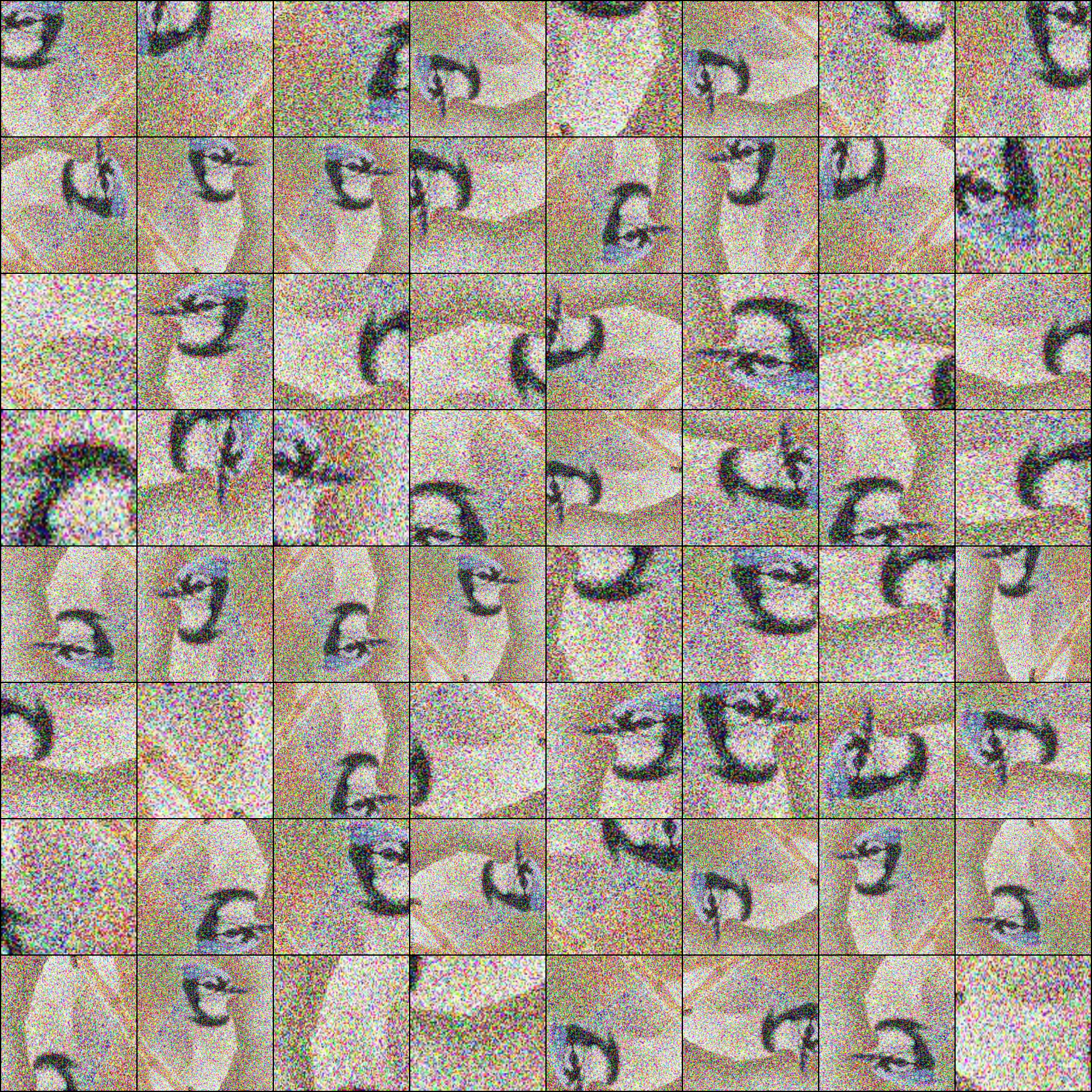
Figure 11: Example of a batch which we create from a single image by augmenting it randomly. The input sample is taken from ImageNet-C [18] (Level 5) Gaussian Noise Corruption.

As evaluated in our ablation study (main manuscript Section 5), augmentations help to further improve the adaptation performance. In our experiments we use random cropping, random horizontal flipping and rotating by specific angles ($0,90,180,270$ degrees). Figure 11 shows an exemplary batch of size 64.

Corruption Benchmarks:

To train the ResNet-26 [16] backbone on CIFAR-10/100 [25], we use a batch size of 128. We train the model for 150 epochs and use Stochastic Gradient Descent (SGD) as optimizer with learning rate 0.1, momentum 0.9 and weight decay $5\cdot 10^{-4}$. We use the multi-step learning rate scheduler from PyTorch with milestones at $75$ and $125$ and set its $\gamma=0.1$. For training we use random cropping and horizontal flipping as augmentations.

Domain Adaptation for Classification:

We use an ImageNet-pretrained ResNet-18 from PyTorch and finetune it on the Office-31 [52] train split. For this finetuning, we train the model for 100 epochs with SGD, initial learning rate $0.1$, momentum $0.9$ and weight decay $5\cdot 10^{-4}$. We use the PyTorch multi-step learning rate scheduler with milestones at $60$ and $75$ and set its $\gamma=0.1$. For VIS-DA [45] we use a ResNet-50, while all other settings are kept the same as for Office-31. We again use random cropping and horizontal flipping as augmentations during training.

Digit Recognition:

For these experiments we use a simple architecture, consisting of 2 convolution layers, 2 linear layers and 2 batch normalization layers. We also use 2 dropout layers in the classification head for regularization with dropout probabilities $p=0.25$ and $p=0.5$, respectively. For each of the datasets, we train this model using ADADELTA [74] for 15 epochs and use a batch size of 64.

Object Detection:

For all our object detection experiments we use a YOLOv3 [49] pretrained on MS-COCO [32]. Then, we retrain the model for 100 epochs on each of the training splits of the respective datasets. We use a batchsize of 20, while all other optimization settings and augmentation routines for training are taken from the PyTorch implementation of YOLOv3.

Appendix B Additional Ablation Results

B.1 Sample Order Does Not Matter

As described in the main manuscript (Section 5), the sample order does not matter. Here, we include the detailed plot for all the 300 runs in Figure 7, which shows that DUA is consistently stable across all runs.

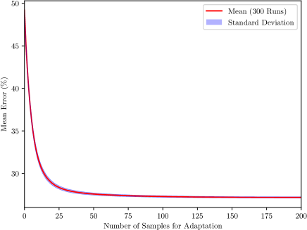
Figure 7: Adaptation results on CIFAR-10C for 300 runs with $\omega=0.94$, $\rho_{0}=0.1$. For each run we randomly shuffle the corrupted test sets. We plot the mean error (on 15 corruptions) and the standard deviation after adaptation on each incoming sample.

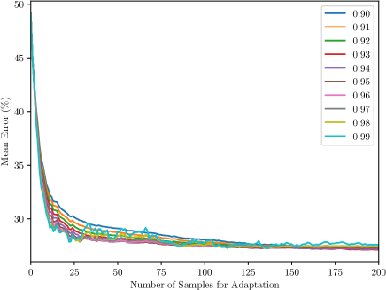
Figure 8: Adaptation results for CIFAR-10C with different values of Momentum Decay Parameter $\omega$. At $\omega=0.94$, we achieve a good balance between stable adaptation and fast convergence. For all these experiments $\rho_{0}=0.1$ is used.

B.2 Choice of Momentum Decay Parameter

The momentum decay parameter $\omega$ helps to provide stable and fast adaptation on the incoming samples. The effect of varying $\omega$ values is analyzed in Figure 8. From this experiment we understand that the adaptation is unstable for a higher value of $\omega$, while it is slower for a lower value. Thus, we use $\omega=0.94$ for all reported experiments, which empirically provides both stable and fast adaptation.

Corruption Type	Abbreviation
Gaussian Noise	gaus
Shot Noise	shot
Impulse Noise	impul
Defocus Blur	defcs
Glass Blur	gls
Motion Blur	mtn
Zoom Blur	zm
Snow	snw
Frost	frst
Fog	fg
Brightness	brt
Contrast	cnt
Elastic	els
Pixelate	px
JPEG Compression	jpg

Table 6: Abbreviations of corruption types in CIFAR-10/100C and ImageNet-C.

Appendix C DUA for Additional Adaptation Tasks

C.1 Domain Adaptation for Digit Recognition

Table 7 summarizes results for cross-dataset domain adaptation in digit recognition. For all these experiments we use a simple architecture consisting of 2 convolution layers, 2 batch normalization layers and 2 fully connected layers. Our method improves the results for all the popular domain adaptation benchmarks. Note that we only use random cropping for digit recognition experiments.

C.2 Domain Adaptation for Visual Recognition

In Table 8, we list the results obtained by testing on two popular domain adaptation benchmarks, Office-31 and VIS-DA. For VIS-DA we take a ResNet-50, pre-trained on ImageNet and then fine tune it on the VIS-DA train split. For the Office-31 dataset, we use an ImageNet pre-trained ResNet-18 which we finetune on the Office-31 train split.

We show that our method achieves improvements on both Office-31 and VIS-DA datasets. It should be noted that the purpose of these evaluations is not to outperform the state-of-the-art methods which specialize on these tasks. Instead, we show that DUA is applicable to a variety of tasks and architectures. It can be used as an initial adaptation method before applying other established domain adaptation methods such as [61, 57, 10, 46].

C.3 Corruption Benchmarks

We provide detailed results for the lower severity corruption levels 1–4 (highest severity level 5 is included in the main manuscript) for CIFAR-10C (Table 9), CIFAR-100C (Table 10) and ImageNet-C (Table 11). Note that the abbreviations of the different corruption types are summarized in Table 6. As can be seen from these results, our DUA achieves consistent improvements over all corruption types and severity levels.

C.4 Object Detection

Natural Domain Shifts:

Table LABEL:tab:results-soda10m_day_to_night shows the results for adapting a detector pre-trained on day images only and tested on night images. Table LABEL:tab:results-kitti_to_soda10m and Table LABEL:tab:results-soda10m_to_kitti report the domain adaptation results between KITTI and SODA10M. DUA provides notable gains for all the different scenarios.

Degrading Weather:

We provide results for the lower severity levels of KITTI-Fog and KITTI-Rain [14] in Table 13 (highest severity/lowest visibility is included in the main manuscript). We see that by adapting a model with DUA, the detection performance increases even in lower severities of rain and fog.

Source data:	SVHN [43]	SVHN	MNIST [27]	MNIST	USPS [20]	USPS	Exemplary Images
Target data:	USPS	MNIST	USPS	SVHN	MNIST	SVHN	MNIST	SVHN	USPS
Source only	66	58	78	16	42	09
DUA	71	68	86	33	55	28
Fully Supervised	94	96	95	85	97	91

Table 7: Domain adaptation results (measured by accuracy in %) for digit recognition. All results are obtained by using a simple architecture consisting of 2 convolution layers, 2 fully connected layers and batch normalization layers.

Source data:	Amazon	Amazon	DSLR	DSLR	Webcam	Webcam
Target data:	Webcam	DSLR	Webcam	Amazon	DSLR	Amazon
Source only	38.4	34.3	12.9	61.4	4.2	66.1
DUA	33.2	29.6	05.7	51.9	2.0	59.7
Fully Supervised	27.1	11.3	03.9	34.1	1.2	22.3

(a)

	Classification
	Error (%)
Source only	57.4
DUA	47.2
Fully Supervised	23.7

(b)

Table 8: Domain adaptation results (measured by classification error in %) for a) Office-31 using a ResNet-18 backbone, and for b) VIS-DA using a ResNet-50 backbone.

	gaus	shot	impul	defcs	gls	mtn	zm	snw	frst	fg	brt	cnt	els	px	jpg	mean
Level 4
Source	63.9	53.7	57.0	28.9	58.9	32.4	38.1	25.9	33.9	17.5	10.4	33.7	26.7	40.7	27.2	36.6
TTT	41.5	35.4	39.8	15.0	47.8	19.1	18.4	20.1	24.0	13.5	10.0	14.1	17.7	29.4	24.5	24.7
NORM	40.7	37.4	43.2	16.7	47.4	21.8	20.2	29.9	30.3	19.0	16.1	20.5	26.5	26.6	35.7	28.8
DUA	31.0	27.6	35.8	13.2	40.7	20.3	15.4	22.2	20.6	12.7	10.1	14.8	20.5	18.6	24.6	21.9
Source	24.1	17.1	16.4	06.6	23.5	08.4	07.4	12.2	11.5	08.3	06.2	09.2	10.6	19.4	13.1	12.9
TENT	13.8	11.7	14.3	06.7	18.6	08.2	07.1	10.6	09.7	07.5	06.1	08.4	10.9	08.5	13.2	10.3
DUA	13.7	11.8	13.5	05.9	18.3	07.6	06.6	10.3	09.0	07.4	05.8	07.2	09.9	09.3	13.0	10.0
Level 3
Source	58.0	47.5	38.5	17.7	46.2	32.8	30.6	22.7	31.8	12.6	09.5	19.3	20.7	23.7	24.7	29.1
TTT	37.2	31.6	28.6	11.5	35.8	19.1	15.8	17.8	23.3	11.0	09.1	11.6	14.3	18.9	22.3	20.5
NORM	37.8	35.1	34.7	14.1	38.2	21.7	18.2	27.5	29.0	16.6	15.2	18.6	19.6	21.1	33.3	25.4
DUA	28.3	24.6	27.0	10.4	30.7	20.2	14.4	20.4	19.3	11.0	09.2	12.3	14.6	15.1	23.1	18.7
Source	20.4	14.6	09.7	05.4	12.9	08.6	06.5	09.9	11.4	06.3	05.5	07.2	07.4	09.6	12.1	09.8
TENT	12.6	10.4	10.4	06.0	12.7	08.1	06.7	09.5	09.1	06.7	05.9	07.5	08.4	07.5	12.7	08.9
DUA	12.2	10.5	09.3	05.5	11.9	07.8	06.1	09.1	09.1	06.1	05.4	06.3	07.0	07.4	11.7	08.4
Level 2
Source	43.1	27.8	29.3	10.2	49.5	23.4	22.4	26.4	21.3	10.3	08.7	13.4	14.7	17.9	22.3	22.7
TTT	28.8	20.7	23.0	09.0	36.6	15.4	13.1	20.2	16.9	09.2	08.3	10.2	12.5	14.8	19.7	17.2
NORM	31.0	25.3	28.7	13.5	38.8	18.8	16.3	27.8	23.9	15.4	14.6	17.1	18.7	19.6	30.6	22.7
DUA	22.3	16.8	22.9	09.2	30.3	16.0	12.7	21.5	15.7	09.6	08.7	11.1	12.7	13.3	20.8	16.2
Source	13.4	08.8	08.0	05.1	14.2	06.5	05.8	09.2	08.5	05.3	05.3	06.1	06.5	07.8	10.9	08.1
TENT	10.2	07.6	08.6	05.9	13.0	07.2	06.2	08.1	07.8	06.3	05.8	06.9	07.5	07.0	11.8	08.0
DUA	10.0	07.5	07.6	05.1	12.4	06.4	05.7	08.3	07.3	05.2	05.2	05.7	06.4	06.8	10.9	07.4
Level 1
Source	25.8	18.4	19.0	08.5	51.1	14.7	18.2	15.0	13.8	08.3	08.3	08.7	14.4	11.3	16.5	16.8
TTT	19.1	15.8	16.5	08.0	37.9	11.7	12.2	12.8	11.9	08.2	08.0	08.3	12.6	11.1	15.5	14.0
NORM	24.0	20.9	22.5	13.4	38.1	16.5	15.5	20.5	18.8	14.9	14.0	15.3	19.1	16.9	24.7	19.7
DUA	16.5	13.8	16.6	08.3	30.4	12.4	12.6	14.5	12.2	08.4	08.4	08.8	13.4	11.0	15.9	13.6
Source	08.7	06.5	06.2	04.9	14.1	05.5	05.9	06.4	06.5	04.9	05.0	05.0	06.9	05.8	08.7	06.7
TENT	07.5	06.9	07.2	05.7	12.4	06.2	06.3	06.8	06.5	05.9	05.7	06.0	07.9	06.5	09.1	07.1
DUA	07.3	06.2	06.2	05.1	11.9	05.5	05.8	06.2	06.1	05.1	05.1	05.1	07.0	05.8	08.5	06.5

Table 9: Error (%) for each corruption in CIFAR-10C severity (Level 1–4) is reported. Source refers to results obtained from a model trained on clean train set and tested on corrupted test sets. For a fair comparison with TTT and NORM, ResNet-26 is used. For comparison with TENT we take the Wide-ResNet-40-2 model from their official Github Repository. Lowest error is highlighted for each corruption.

	gaus	shot	impul	defcs	gls	mtn	zm	snw	frst	fg	brt	cnt	els	px	jpg	mean
Level 4
Source	88.3	85.3	92.8	54.3	84.8	57.3	57.2	54.9	65.9	48.6	35.8	61.1	52.9	73.0	61.0	64.9
TTT	81.6	78.3	81.1	48.6	78.7	52.5	53.4	53.8	62.8	49.5	38.5	50.3	50.2	66.2	57.2	60.2
NORM	70.5	67.6	72.1	41.1	69.9	46.1	44.5	54.7	55.2	46.7	38.8	44.1	50.8	49.9	64.2	54.4
DUA	66.0	62.9	66.4	41.3	66.5	48.2	43.0	53.5	52.8	43.2	37.6	45.7	48.2	46.6	57.6	52.0
Source	60.7	51.6	47.9	27.1	54.4	30.3	28.9	37.4	39.0	35.4	27.2	35.9	34.4	39.0	40.1	39.3
TENT	38.9	36.3	36.6	27.3	42.0	28.9	28.4	34.8	32.8	32.1	26.3	29.8	33.3	29.9	38.4	33.1
DUA	43.0	39.0	37.9	26.9	44.7	29.5	28.3	36.5	34.3	33.8	26.6	31.0	33.8	31.0	38.9	34.3
Level 3
Source	86.0	81.4	83.8	42.7	78.3	57.7	52.4	53.0	64.1	40.1	33.3	49.3	46.6	54.4	58.2	58.8
TTT	79.6	74.6	69.3	42.5	73.0	53.2	49.8	51.2	61.4	42.1	36.8	43.5	45.8	52.9	55.2	55.4
NORM	67.7	64.6	62.3	60.9	63.4	42.6	52.6	54.5	41.5	37.8	37.8	41.1	44.3	45.0	61.7	51.9
DUA	63.8	60.0	57.9	37.3	58.4	48.2	41.2	50.8	52.4	39.2	35.5	41.4	41.7	42.1	55.3	48.4
Source	55.2	45.9	36.9	25.7	39.9	30.5	27.4	33.3	38.1	29.5	25.5	30.5	28.6	30.3	38.0	34.4
TENT	37.1	34.3	32.0	26.1	34.6	29.2	27.7	32.3	32.3	29.0	25.6	28.4	29.2	28.3	37.4	30.9
DUA	40.8	36.5	32.2	25.3	37.0	29.6	27.1	32.7	34.4	29.0	25.2	28.6	28.4	28.7	37.3	31.5
Level 2
Source	79.9	66.1	73.7	33.7	79.6	48.9	46.4	56.8	52.4	35.2	31.3	42.1	40.5	48.0	55.2	52.7
TTT	71.5	61.8	59.8	36.5	73.1	47.2	46.0	55.7	52.8	38.0	35.2	39.7	42.0	47.9	52.6	50.7
NORM	61.1	54.9	55.9	36.3	61.1	43.0	40.7	53.0	49.0	39.6	37.0	39.5	42.8	43.3	59.0	47.7
DUA	57.1	50.7	52.0	35.2	58.4	43.8	39.1	52.8	47.6	35.9	34.2	38.9	39.9	39.7	52.9	45.2
Source	44.6	34.5	30.7	24.3	41.5	27.7	26.2	32.7	31.8	26.8	24.4	27.5	27.9	28.0	36.5	31.0
TENT	33.3	29.5	28.8	25.7	34.9	27.4	27.0	30.6	29.6	27.0	25.4	27.3	29.1	27.6	36.3	29.3
DUA	35.9	31.2	28.8	24.1	36.9	27.2	26.0	32.2	30.9	26.1	24.0	26.6	27.9	27.6	35.9	29.4
Level 1
Source	65.0	53.4	54.2	30.3	80.1	40.2	42.9	39.6	43.0	31.0	30.2	31.8	40.3	37.0	48.1	44.5
TTT	60.4	53.0	48.0	34.7	74.0	41.3	41.3	41.5	44.2	34.6	34.4	34.8	41.8	39.4	47.0	44.7
NORM	52.9	48.8	47.7	36.2	60.6	40.1	39.5	43.9	44.0	36.8	36.3	36.7	43.2	40.6	52.0	44.0
DUA	49.6	45.5	44.4	32.5	58.0	39.4	38.3	41.7	41.9	33.2	33.1	33.5	40.8	36.0	47.0	41.0
Source	34.4	29.6	26.9	23.8	42.9	25.6	26.1	26.1	27.4	24.0	23.8	24.3	28.4	25.2	32.4	28.1
TENT	29.3	27.6	26.9	25.5	34.7	26.6	26.7	27.0	27.3	25.6	25.2	26.0	29.8	26.7	32.9	27.9
DUA	31.2	28.5	26.4	23.8	36.9	25.3	25.9	26.2	27.1	24.1	23.9	23.9	28.6	25.4	32.0	27.3

Table 10: Error (%) for each corruption in CIFAR-100C severity (Level 1–4) is reported. Source refers to results obtained from a model trained on clean train set and tested on corrupted test sets. For a fair comparison with TTT and NORM, ResNet-26 is used. For comparison with TENT we take the Wide-ResNet-40-2 model from their official Github Repository. Lowest error is highlighted for each corruption.

	gaus	shot	impul	defcs	gls	mtn	zm	snw	frst	fg	brt	cnt	els	px	jpg	mean
Level 4
Source	93.2	94.7	94.3	84.5	89.4	85.3	77.2	83.4	79.4	72.8	44.5	88.1	63.4	71.2	58.8	78.7
NORM	84.4	77.6	87.3	86.4	88.0	76.8	70.7	76.9	70.9	56.0	37.8	64.4	53.5	58.6	57.8	69.8
DUA	78.1	82.8	80.3	82.8	83.3	78.7	69.8	76.1	74.2	59.7	40.4	87.3	55.8	61.8	54.9	71.1
Level 3
Source	80.9	82.7	82.9	74.1	85.4	73.9	71.9	73.6	77.8	66.2	39.6	65.3	51.1	56.7	49.3	68.8
NORM	65.5	69.8	63.2	71.1	79.5	63.6	58.2	68.1	65.4	55.3	39.3	55.0	41.0	51.8	50.9	59.8
DUA	67.6	68.5	69.0	70.7	78.6	66.4	65.3	66.9	70.6	54.3	37.4	61.8	46.5	47.6	48.2	61.3
Level 2
Source	63.6	67.8	74.6	59.4	65.4	57.7	65.2	77.5	67.0	56.3	36.4	51.5	60.9	43.3	46.3	59.5
NORM	50.7	61.2	65.2	61.3	54.4	46.4	55.8	69.1	58.0	45.6	36.1	40.3	64.1	41.3	40.6	52.7
DUA	56.4	58.0	62.0	56.5	62.0	53.1	58.0	69.9	63.0	49.3	35.8	50.5	56.6	40.6	45.3	54.5
Level 1
Source	50.5	53.1	61.9	51.3	52.4	45.2	55.9	55.5	49.7	49.0	34.2	44.0	40.4	41.3	42.6	48.5
NORM	47.0	48.4	54.1	50.2	47.8	39.5	50.3	47.7	44.1	41.1	38.4	36.6	42.0	37.0	43.2	44.5
DUA	45.7	49.0	54.7	50.6	49.8	43.4	50.1	51.7	46.9	45.8	31.8	43.3	38.9	39.1	41.5	45.5

Table 11: Error (%) for each corruption in ImageNet-C severity (Level 1–4) is reported. Source refers to results obtained from a model pre-trained on ImageNet and tested on corrupted test sets. All results are obtained by using ResNet-18 as the backbone architecture. Lowest error is highlighted for each corruption.

	Car	Ped	Cyclist
SO	75.3	48.3	50.1
DUA	77.2	49.9	51.6
FS	86.9	55.7	63.2

(a)

	Car	Ped	Cyclist
SO	43.6	13.9	18.9
DUA	49.4	17.2	23.1
FS	84.8	46.1	61.2

(b)

	Car	Ped	Cyclist
SO	80.1	55.5	33.9
DUA	81.3	56.3	35.1
FS	91.8	71.3	76.5

(c)

Table 12: Domain adaptation results (mAP@50) for object detection with YOLOv3. a) We train on the SODA10M day split and test on the SODA10M night split. b) We train on the KITTI train split and test on the SODA10M test split. c) We train on the SODA10M day split and test on the KITTI validation split (details in Table 5). SO: source-only, FS: fully supervised.

	Car	Pedestrian	Cyclist
40m fog visibility
Source only	39.6	39.3	20.2
DUA	61.3	53.5	39.9
Fully Supervised	77.8	68.1	70.5
50m fog visibility
Source only	48.2	45.9	27.3
DUA	69.6	59.7	48.4
Fully Supervised	82.2	71.3	74.2

(a)

	Car	Pedestrian	Cyclist
100 mm/hr rain
Source only	93.2	80.5	81.1
DUA	94.9	81.7	83.2
Fully Supervised	95.4	83.2	84.1
75 mm/hr rain
Source only	95.5	82.6	83.6
DUA	96.1	83.2	86.0
Fully Supervised	96.6	84.1	87.2

(b)

Table 13: Results for KITTI pretrained YOLOv3 tested on rain and fog datasets. Mean Average Precision (mAP@50) is reported for the three common classes in KITTI dataset. a) Results for $40$m and $50$m visibility in fog. b) Results for $100$mm/hr and $75$mm/hr rain intensity.

References

- [1] Matteo Biasetton, Umberto Michieli, Gianluca Agresti, and Pietro Zanuttigh. Unsupervised Domain Adaptation for Semantic Segmentation of Urban Scenes. In Proc. CVPRW, 2019.
- [2] Chao Chen, Zhihang Fu, Zhihong Chen, Sheng Jin, Zhaowei Cheng, Xinyu Jin, and Xian-Sheng Hua. HoMM: Higher-order Moment Matching for Unsupervised Domain Adaptation. In Proc. AAAI, 2020.
- [3] Hongruixuan Chen, Chen Wu, Yonghao Xu, and Bo Du. Unsupervised Domain Adaptation for Semantic Segmentation via Low-level Edge Information Transfer. arXiv preprint arXiv:2109.08912, 2021.
- [4] Yuhua Chen, Wen Li, Christos Sakaridis, Dengxin Dai, and Luc Van Gool. Domain Adaptive Faster R-CNN for Object Detection in the Wild. In Proc. CVPR, 2018.
- [5] Yi-Hsin Chen, Wei-Yu Chen, Yu-Ting Chen, Bo-Cheng Tsai, Yu-Chiang Frank Wang, and Min Sun. No More Discrimination: Cross City Adaptation of Road Scene Segmenters. In Proc. ICCV, 2017.
- [6] Sumit Chopra, Raia Hadsell, and Yann LeCun. Learning a Similarity Metric Discriminatively, with Application to Face Verification. In Proc. CVPR, 2005.
- [7] Jia Deng, Wei Dong, Richard Socher, Li-Jia Li, Kai Li, and Li Fei-Fei. Imagenet: A Large-scale Hierarchical Image Database. In Proc. CVPR, 2009.
- [8] Christian Fruhwirth-Reisinger, Michael Opitz, Horst Possegger, and Horst Bischof. FAST3D: Flow-Aware Self-Training for 3D Object Detectors. In Proc. BMVC, 2021.
- [9] Angus Galloway, Anna Golubeva, Thomas Tanay, Medhat Moussa, and Graham W Taylor. Batch Normalization is a Cause of Adversarial Vulnerability. arXiv preprint arXiv:1905.02161, 2019.
- [10] Yaroslav Ganin, Evgeniya Ustinova, Hana Ajakan, Pascal Germain, Hugo Larochelle, François Laviolette, Mario Marchand, and Victor Lempitsky. Domain-Adversarial Training of Neural Networks. JMLR, 17(59):1–35, 2016.
- [11] Andreas Geiger, Philip Lenz, Christoph Stiller, and Raquel Urtasun. Vision meets Robotics: The KITTI Dataset. IJR, 32(11):1231–1237, 2013.
- [12] Spyros Gidaris, Praveer Singh, and Nikos Komodakis. Unsupervised Representation Learning by Predicting Image Rotations. In Proc. ICLR, 2018.
- [13] Ian Goodfellow, Jean Pouget-Abadie, Mehdi Mirza, Bing Xu, David Warde-Farley, Sherjil Ozair, Aaron Courville, and Yoshua Bengio. Generative Adversarial Nets. In NeurIPS, 2014.
- [14] Shirsendu Sukanta Halder, Jean-François Lalonde, and Raoul de Charette. Physics-based Rendering for Improving Robustness to Rain. In Proc. ICCV, 2019.
- [15] Jianhua Han, Xiwen Liang, Hang Xu, Kai Chen, Lanqing Hong, Chaoqiang Ye, Wei Zhang, Zhenguo Li, Chunjing Xu, and Xiaodan Liang. SODA10M: Towards Large-Scale Object Detection Benchmark for Autonomous Driving. In NeurIPS, 2021.
- [16] Kaiming He, Xiangyu Zhang, Shaoqing Ren, and Jian Sun. Deep Residual Learning for Image Recognition. In Proc. CVPR, 2016.
- [17] Zhenwei He and Lei Zhang. Multi-adversarial Faster-RCNN for Unrestricted Object Detection. In Proc. ICCV, 2019.
- [18] Dan Hendrycks and Thomas Dietterich. Benchmarking Neural Network Robustness to Common Corruptions and Perturbations. In Proc. ICLR, 2019.
- [19] Weixiang Hong, Zhenzhen Wang, Ming Yang, and Junsong Yuan. Conditional Generative Adversarial Network for Structured Domain Adaptation. In Proc. CVPR, 2018.
- [20] Jonathan J. Hull. A Database for Handwritten Text Recognition Research. TPAMI, 16(5):550–554, 1994.
- [21] Sergey Ioffe and Christian Szegedy. Batch Normalization: Accelerating Deep Network Training by Reducing Internal Covariate Shift. In Proc. ICML, 2015.
- [22] Maximilian Jaritz, Tuan-Hung Vu, Raoul de Charette, Emilie Wirbel, and Patrick Pérez. xMUDA: Cross-Modal Unsupervised Domain Adaptation for 3D Semantic Segmentation. In Proc. CVPR, 2020.
- [23] Guoliang Kang, Lu Jiang, Yi Yang, and Alexander G Hauptmann. Contrastive Adaptation Network for Unsupervised Domain Adaptation. In Proc. CVPR, 2019.
- [24] Taekyung Kim, Minki Jeong, Seunghyeon Kim, Seokeon Choi, and Changick Kim. Diversify and Match: A Domain Adaptive Representation Learning Paradigm for Object Detection. In Proc. CVPR, 2019.
- [25] Alex Krizhevsky and Geoffrey Hinton. Learning Multiple Layers of Features from Tiny Images. Technical report, Department of Computer Science, University of Toronto, 2009.
- [26] Alex Krizhevsky, Ilya Sutskever, and Geoffrey E Hinton. ImageNet Classification with Deep Convolutional Neural Networks. In NeurIPS, 2012.
- [27] Yann LeCun, Léon Bottou, Yoshua Bengio, and Patrick Haffner. GradientBased Learning Applied to Document Recognition. In Proc. IEEE, 1998.
- [28] Yanghao Li, Naiyan Wang, Jianping Shi, Jiaying Liu, and Xiaodi Hou. Revisiting Batch Normalization For Practical Domain Adaptation. In Proc. ICLRW, 2016.
- [29] Qing Lian, Fengmao Lv, Lixin Duan, and Boqing Gong. Constructing Self-motivated Pyramid Curriculums for Cross-Domain Semantic Segmentation: A Non-Adversarial Approach. In Proc. ICCV, 2019.
- [30] J. Liang et al. Do We Really Need to Access the Source Data? Source Hypothesis Transfer for Unsupervised Domain Adaptation. In ICML, 2020.
- [31] Tsung-Yi Lin, Priya Goyal, Ross Girshick, Kaiming He, and Piotr Dollár. Focal Loss for Dense Object Detection. In Proc. ICCV, 2017.
- [32] Tsung-Yi Lin, Michael Maire, Serge Belongie, James Hays, Pietro Perona, Deva Ramanan, Piotr Dollár, and C Lawrence Zitnick. Microsoft COCO: Common Objects in Context. In Proc. ECCV, 2014.
- [33] Hong Liu, Mingsheng Long, Jianmin Wang, and Michael Jordan. Transferable Adversarial Training: A General Approach to Adapting Deep Classifiers. In Proc. ICML, 2019.
- [34] Ming-Yu Liu and Oncel Tuzel. Coupled Generative Adversarial Networks. In NeurIPS, 2016.
- [35] Wei Liu, Dragomir Anguelov, Dumitru Erhan, Christian Szegedy, Scott Reed, Cheng-Yang Fu, and Alexander C Berg. SSD: Single Shot MultiBox Detector. In Proc. ECCV, 2016.
- [36] Xiaofeng Liu, Site Li, Yubin Ge, Pengyi Ye, Jane You, and Jun Lu. Recursively Conditional Gaussian for Ordinal Unsupervised Domain Adaptation. In Proc. ICCV, 2021.
- [37] Mingsheng Long, Yue Cao, Jianmin Wang, and Michael Jordan. Learning Transferable Features with Deep Adaptation Networks. In Proc. ICML, 2015.
- [38] Yawei Luo, Liang Zheng, Tao Guan, Junqing Yu, and Yi Yang. Taking A Closer Look at Domain Shift: Category-level Adversaries for Semantics Consistent Domain Adaptation. In Proc. CVPR, 2019.
- [39] Fabio Maria Carlucci, Lorenzo Porzi, Barbara Caputo, Elisa Ricci, and Samuel Rota Bulo. AutoDIAL: Automatic DomaIn Alignment Layers. In Proc. ICCV, 2017.
- [40] Claudio Michaelis, Benjamin Mitzkus, Robert Geirhos, Evgenia Rusak, Oliver Bringmann, Alexander S Ecker, Matthias Bethge, and Wieland Brendel. Benchmarking Robustness in Object Detection: Autonomous Driving when Winter is Coming. arXiv preprint arXiv:1907.07484, 2019.
- [41] Muhammad Jehanzeb Mirza, Cornelius Buerkle, Julio Jarquin, Michael Opitz, Fabian Oboril, Kay-Ulrich Scholl, and Horst Bischof. Robustness of Object Detectors in Degrading Weather Conditions. In Proc. ITSC, 2021.
- [42] Zachary Nado, Shreyas Padhy, D Sculley, Alexander D’Amour, Balaji Lakshminarayanan, and Jasper Snoek. Evaluating Prediction-Time Batch Normalization for Robustness under Covariate Shift. arXiv preprint arXiv:2006.10963, 2020.
- [43] Yuval Netzer, Tao Wang, Adam Coates, Alessandro Bissacco, Bo Wu, and Andrew Y Ng. Reading Digits in Natural Images with Unsupervised Feature Learning. In NeurIPS, 2011.
- [44] Adam Paszke, Sam Gross, Francisco Massa, Adam Lerer, James Bradbury, Gregory Chanan, Trevor Killeen, Zeming Lin, Natalia Gimelshein, Luca Antiga, Alban Desmaison, Andreas Kopf, Edward Yang, Zachary DeVito, Martin Raison, Alykhan Tejani, Sasank Chilamkurthy, Benoit Steiner, Lu Fang, Junjie Bai, and Soumith Chintala. PyTorch: An Imperative Style, High-Performance Deep Learning Library. In NeurIPS, 2019.
- [45] Xingchao Peng, Ben Usman, Neela Kaushik, Judy Hoffman, Dequan Wang, and Kate Saenko. VisDA: A Synthetic-to-Real Benchmark for Visual Domain Adaptation. In Proc. CVPRW, 2017.
- [46] Pedro O Pinheiro. Unsupervised Domain Adaptation with Similarity Learning. In Proc. CVPR, 2018.
- [47] Can Qin, Haoxuan You, Lichen Wang, C-C Jay Kuo, and Yun Fu. PointDAN: A Multi-Scale 3D Domain Adaption Network for Point Cloud Representation. In NeurIPS, 2019.
- [48] Benjamin Recht, Rebecca Roelofs, Ludwig Schmidt, and Vaishaal Shankar. Do ImageNet Classifiers Generalize to ImageNet? In Proc. ICML, 2019.
- [49] Joseph Redmon and Ali Farhadi. YOLOv3: An Incremental Improvement. arXiv preprint arXiv:1804.02767, 2018.
- [50] Shaoqing Ren, Kaiming He, Ross Girshick, and Jian Sun. Faster R-CNN: Towards Real-Time Object Detection with Region Proposal Networks. In NeurIPS, 2015.
- [51] David E Rumelhart, Geoffrey E Hinton, and Ronald J Williams. Learning Representations by Back-propagating Errors. Nature, 323(6088):533–536, 1986.
- [52] Kate Saenko, Brian Kulis, Mario Fritz, and Trevor Darrell. Adapting Visual Category Models to New Domains. In Proc. ECCV, 2010.
- [53] Kuniaki Saito, Yoshitaka Ushiku, Tatsuya Harada, and Kate Saenko. Strong-Weak Distribution Alignment for Adaptive Object Detection. In Proc. CVPR, 2019.
- [54] Shibani Santurkar, Dimitris Tsipras, Andrew Ilyas, and Aleksander Mądry. How Does Batch Normalization Help Optimization? In NeurIPS, 2018.
- [55] Steffen Schneider, Evgenia Rusak, Luisa Eck, Oliver Bringmann, Wieland Brendel, and Matthias Bethge. Improving Robustness Against Common Corruptions by Covariate Shift Adaptation. In NeurIPS, 2020.
- [56] Saurabh Singh and Abhinav Shrivastava. EvalNorm: Estimating Batch Normalization Statistics for Evaluation. In Proc. ICCV, 2019.
- [57] Baochen Sun, Jiashi Feng, and Kate Saenko. Return of Frustratingly Easy Domain Adaptation. In Proc. AAAI, 2016.
- [58] Baochen Sun and Kate Saenko. Deep CORAL: Correlation Alignment for Deep Domain Adaptation. In Proc. ECCVW, 2016.
- [59] Pei Sun, Henrik Kretzschmar, Xerxes Dotiwalla, Aurelien Chouard, Vijaysai Patnaik, Paul Tsui, James Guo, Yin Zhou, Yuning Chai, Benjamin Caine, et al. Scalability in Perception for Autonomous Driving: Waymo Open Dataset. In Proc. CVPR, 2020.
- [60] Yu Sun, Eric Tzeng, Trevor Darrell, and Alexei A Efros. Unsupervised Domain Adaptation through Self-Supervision. arXiv preprint arXiv:1909.11825, 2019.
- [61] Yu Sun, Xiaolong Wang, Zhuang Liu, John Miller, Alexei Efros, and Moritz Hardt. Test-Time Training with Self-Supervision for Generalization under Distribution Shifts. In Proc. ICML, 2020.
- [62] Mingxing Tan, Ruoming Pang, and Quoc V Le. EfficientDet: Scalable and Efficient Object Detection. In Proc. CVPR, 2020.
- [63] Eric Tzeng, Judy Hoffman, Kate Saenko, and Trevor Darrell. Adversarial Discriminative Domain Adaptation. In Proc. CVPR, 2017.
- [64] Dequan Wang, Evan Shelhamer, Shaoteng Liu, Bruno Olshausen, and Trevor Darrell. Tent: Fully Test-time Adaptation by Entropy Minimization. In Proc. ICLR, 2020.
- [65] Rui Wang, Zuxuan Wu, Zejia Weng, Jingjing Chen, Guo-Jun Qi, and Yu-Gang Jiang. Cross-domain Contrastive Learning for Unsupervised Domain Adaptation. arXiv preprint arXiv:2106.05528, 2021.
- [66] Yan Wang, Xiangyu Chen, Yurong You, Li Erran Li, Bharath Hariharan, Mark Campbell, Kilian Q Weinberger, and Wei-Lun Chao. Train in Germany, Test in The USA: Making 3D Object Detectors Generalize. In Proc. CVPR, 2020.
- [67] Yuxin Wu and Justin Johnson. Rethinking “Batch” in BatchNorm. arXiv preprint arXiv:2105.07576, 2021.
- [68] Rongchang Xie, Fei Yu, Jiachao Wang, Yizhou Wang, and Li Zhang. Multi-Level Domain Adaptive Learning for Cross-Domain Detection. In Proc. ICCVW, 2019.
- [69] Saining Xie, Ross Girshick, Piotr Dollár, Zhuowen Tu, and Kaiming He. Aggregated Residual Transformations for Deep Neural Networks. In Proc. CVPR, 2017.
- [70] Qiangeng Xu, Yin Zhou, Weiyue Wang, Charles R Qi, and Dragomir Anguelov. SPG: Unsupervised Domain Adaptation for 3D Object Detection via Semantic Point Generation. In Proc. ICCV, 2021.
- [71] Jihan Yang, Shaoshuai Shi, Zhe Wang, Hongsheng Li, and Xiaojuan Qi. ST3D: Self-training for Unsupervised Domain Adaptation on 3D Object Detection. In Proc. CVPR, 2021.
- [72] Fei Yu, Mo Zhang, Hexin Dong, Sheng Hu, Bin Dong, and Li Zhang. DAST: Unsupervised Domain Adaptation in Semantic Segmentation Based on Discriminator Attention and Self-Training. In Proc. AAAI, 2021.
- [73] Sergey Zagoruyko and Nikos Komodakis. Wide Residual Networks. In Proc. BMVC, 2016.
- [74] Matthew D Zeiler. ADADELTA: An Adaptive Learning Rate Method. arXiv preprint arXiv:1212.5701, 2012.
- [75] Werner Zellinger, Thomas Grubinger, Edwin Lughofer, Thomas Natschläger, and Susanne Saminger-Platz. Central Moment Discrepancy (CMD) for Domain-Invariant Representation Learning. In Proc. ICLR, 2017.
- [76] M. Zhang, H. Marklund, N. Dhawan, A. Gupta, S. Levine, and C. Finn. Adaptive risk minimization: Learning to adapt to domain shift. In NeurIPS, 2021.
- [77] Yangtao Zheng, Di Huang, Songtao Liu, and Yunhong Wang. Cross-domain Object Detection through Coarse-to-Fine Feature Adaptation. In Proc. CVPR, 2020.
- [78] Yang Zou, Zhiding Yu, BVK Kumar, and Jinsong Wang. Unsupervised Domain Adaptation for Semantic Segmentation via Class-Balanced Self-Training. In Proc. ECCV, 2018.