A General Approach for Lookback Option Pricing under Markov Models

Abstract

We propose a very efficient method for pricing various types of lookback options under Markov models. We utilize the model-free representations of lookback option prices as integrals of first passage probabilities. We combine efficient numerical quadrature with continuous-time Markov chain approximation for the first passage problem to price lookbacks. Our method is applicable to a variety of models, including one-dimensional time-homogeneous and time-inhomogeneous Markov processes, regime-switching models and stochastic local volatility models. We demonstrate the efficiency of our method through various numerical examples.

Keywords: lookback options, drawdown, Markov chain approximation, Gauss quadrature.

1 Introduction

Lookback options are an important class of path-dependent derivatives in financial markets, and they can be monitored continuously or discretely (the maximum price is calculated from a discrete set of dates). The pricing of lookback options has been extensively studied. Fusai (2010) provides a comprehensive review of the topic. Under the Black-Scholes model, analytical solutions for different types of continuous lookback options are derived in Goldman et al. (1979) and Conze (1991), while for discrete lookback options several numerical methods are put forth, including binomial/trinomial trees (Cheuk and Vorst (1997), Babbs (2000), Dai (2000), Tse et al. (2001)), continuity correction (Broadie et al. (1999)), a numerical integration scheme based on random walk duality (Aitsahlia and Lai (1998)), double-exponential fast Gauss transform (Broadie and Yamamoto (2005)) and $z$-transform (Atkinson and Fusai (2007), Green et al. (2010)). For the CEV model, Davydov and Linetsky (2001) price continuous lookback options by numerically inverting Laplace transform and Boyle and Tian (1999) employ trinomial trees. Furthermore, Linetsky (2004) proposes a spectral expansion approach that is applicable to a class of one-dimensional diffusions. For one-dimensional exponential Lévy models that can have jumps, Boyarchenko and Levendorskiǐ (2013) devise a method based on Wiener-Hopf factorization for continuous lookback options, whereas Petrella and Kou (2004), Feng and Linetsky (2009) and Fusai et al. (2016) develop methods based on Laplace transform, Hilbert transform, and a combination of $z$-transform and Hilbert transform for discretely monitored ones. Additionally, a numerical PDE approach based on finite element is pursued in Forsyth et al. (1999) for some stochastic volatility models. Last but not the least, Monte Carlo simulation techniques are discussed in Glasserman (2013) for discrete lookback options.

In this paper, we propose a new computational method for pricing lookback options based on continuous-time Markov chain (CTMC) approximation for general Markov models. CTMC approximation has become a popular method for solving various option pricing problems under Markov models in recent years. See Mijatović and Pistorius (2013) and Cui and Taylor (2021) for barrier options, Eriksson and Pistorius (2015) for American options, Cai et al. (2015), Song et al. (2018) and Cui et al. (2018) for Asian options, Zhang and Li (2021c) for maximum drawdown options, Zhang et al. (2021) for American drawdown options, Zhang and Li (2021b) for Parisian options, and Meier et al. (2021) for option pricing under financial models with sticky behavior. In all these papers, the original Markov model is approximated by a CTMC, and then the option price under the CTMC model is derived. We can follow this approach to derive the lookback option price under a CTMC model. However, this algorithm is inferior in terms of computational efficiency to alternatives generated by our method (see Remark 2 for the explanation). In our approach, we combine CTMC approximation with numerical quadrature. We utilize the model-free representation that expresses the lookback option price as an integral of first passage probabilities. We apply a quadrature rule to discretize the integral and calculate each first passage probability by CTMC approximation. By using an efficient quadrature rule, our method can yield an efficient algorithm for pricing lookback options. Other applications of efficient quadrature rules for option pricing can be found in Andricopoulos et al. (2003), Andricopoulos et al. (2007), Fusai and Recchioni (2007).

Our method has two nice features. First, it is applicable to very general models, including one-dimensional (1D) time-homogeneous and time-inhomogeneous Markov processes, regime-switching models and stochastic local volatility models. Second, it can generate very efficient algorithms by using efficient quadrature rules. In particular, using the Gauss-Legendre quadrature, we can obtain highly accurate results with a small or moderate number of quadrature points. In one example, we show that our method significantly outperforms the finite difference method for solving the partial differential equation for the lookback option price.

The rest of the paper is organized as follows. Section 2 first reviews the model-free representations for lookback options and CTMC approximation for the first-passage problem and then presents our algorithm. Section 3 develops convergence rate analysis for our algorithm under 1D diffusion models. Section 4 provides various numerical examples to demonstrate the efficiency and convergence of our algorithm. Section 5 concludes.

2 Lookback Option Pricing

Let $X_{t}$ denote the underlying asset price at time $t$. Define $m_{t}=\inf_{0\leq u\leq t}X_{u}$, and $M_{t}=\sup_{0\leq u\leq t}X_{u}$, which are the running minimum and maximum of the price process starting from time $0$, respectively. We also consider the seasoned running minimum and maximum $\overline{m}_{t}=\overline{m}_{0}\wedge m_{t}$, $\overline{M}_{t}=\overline{M}_{0}\vee M_{t}$, where $\overline{m}_{0}$ and $\overline{M}_{0}$ are the minimum and maximum before time $0$.

We consider four types of standard lookback options and focus on continuous monitoring in this paper (see Remark 1 for how to treat discretely monitored ones in our algorithm). In the following, we consider general seasoned lookback options that mature at $T$ and price them at $t\in[0,T]$. Define $\tau:=T-t$ and let $r,d$ be the constant risk-free rate and dividend yield, respectively. Davydov and Linetsky (2001) shows that their prices admit the following model-free representations:

• Floating-strike lookback put:

  $$u^{flp}(t,x,M) =e^{-r\tau}\mathbb{E}\left[\left(\overline{M}_{T}-X_{T}\right)^{+}|X_{t}=x,\overline{M}_{t}=M\right]$$ (1)

  $$=e^{-r\tau}M-e^{-d\tau}x+e^{-r\tau}\int_{M}^{\infty}P_{x}\left(M_{\tau}\geq y\right)dy.$$ (2)

  It’s worth noticing that the floating-strike lookback put is an option that compensates the option holder the drawdown of the asset at maturity. This type of options becomes particularly relevant in market turmoil.

• Floating-strike lookback call:

  $$u^{flc}(t,x,m) =e^{-r\tau}\mathbb{E}\left[\left(X_{T}-\overline{m}_{T}\right)^{+}|X_{t}=x,\overline{m}_{t}=m\right]$$ (3)

  $$=e^{-d\tau}x-e^{-r\tau}m+e^{-r\tau}\int_{0}^{m}P_{x}\left(m_{\tau}\leq y\right)dy.$$ (4)

• Fixed-strike lookback put:

  $$u^{fip}(t,x,m) =e^{-r\tau}\mathbb{E}\left[\left(K-\overline{m}_{T}\right)^{+}|X_{t}=x,\overline{m}_{t}=m\right]$$ (5)

  $$=e^{-r\tau}(K-m)^{+}+e^{-r\tau}\int_{0}^{m\wedge K}P_{x}\left(m_{\tau}\leq y\right)dy.$$ (6)

• Fixed-strike lookback call:

  $$u^{fic}(t,x,M) =e^{-r\tau}\mathbb{E}\left[\left(\overline{M}_{T}-K\right)^{+}|X_{t}=x,\overline{M}_{t}=M\right]$$ (7)

  $$=e^{-r\tau}(M-K)^{+}+e^{-r\tau}\int_{M\vee K}^{\infty}P_{x}\left(M_{\tau}\geq y\right)dy.$$ (8)

The distributions of $m_{\tau}$ and $M_{\tau}$ are essetially first passage probabilities. Using these representations, the lookback option pricing problem boils down to calculating the intergral of first passage probabilities for different passage levels. It is important to note that these probabilities are for the unseasoned running minimum and maximum, thus the seasoned problem has been turned into an unseasoned one. A general and efficient method for the first passage probability calculation is CTMC approximation, which we review in the next subsection.

2.1 CTMC Approximation for the First Passage Problem

Consider a 1D time-homogeneous Markov model for the asset price process $X_{t}$. In financial models, $X_{t}$ lives on the continuous state space $\mathbb{R}^{+}$. We can approximate $X_{t}$ by CTMCs and we refer readers to e.g., Mijatović and Pistorius (2013), Section 4 or Zhang and Li (2021c), Appendix A for the construction of CTMC approximation for diffusions, jump-diffusions and pure-jump models. Let $\{Y^{(n)}_{t}\}$ is a sequence of CTMCs that converges weakly to $X_{t}$. For $Y^{(n)}_{t}$, it lives on the state space $\mathbb{S}^{(n)}=\{s^{(n)}_{0},\cdots,s^{(n)}_{n}\}$ with $n+1$ grid points and $\delta_{n}$ is the mesh size. Hereafter, all quantities with superscript $(n)$ are defined for $Y^{(n)}_{t}$ in the same way as those defined for $X_{t}$.

For $Y^{(n)}_{t}$, we denote its generator matrix by $G_{n}$ with $G_{n}(x,y)$ referring to the transition rate from state $x$ to $y$. Let $p_{n}(t,x,y):=P(Y^{(n)}_{t}=y|Y^{(n)}_{0}=x)$. As $t\to 0$, $p_{n}(t,x,y)=1_{\{x=y\}}+G_{n}(x,y)t+o(t)$. It is a classical result that $p_{n}(t,x,y)=(\exp{(G_{n}t)})(x,y)$ (Serfozo (2009), Section 4.4), where $\exp{(A)}$ is the matrix exponential of matrix $A$ defined as

$$\exp{(A)}=\sum_{n=0}^{\infty}\frac{A^{n}}{n!}.$$ (9)

Consider the first passage times of $Y^{(n)}_{t}$ defined as

$$T_{y}^{(n),+(-)}=\inf\{t\geq 0:Y^{(n)}_{t}>(<)y\}.$$ (10)

Closed-form formulas for first passage probabilities under CTMCs with finite state spaces were derived in Mijatović and Pistorius (2013). Let $G_{n,\leq y}$ be the square sub-matrix of $G_{n}$ by keeping only transition rates among states in the space $\{z\in\mathbb{S}^{(n)}:z\leq y\}$ and define $G_{n,\geq y}$ similarly. Then, we have

$$P_{x}(T_{y}^{(n),+}>t) =(\exp{(G_{n,\leq y}t)}{\boldsymbol{1}})(x),$$ (11)

$$P_{x}(T_{y}^{(n),-}>t) =(\exp{(G_{n,\geq y}t)}{\boldsymbol{1}})(x).$$ (12)

where ${\boldsymbol{1}}$ is a vector of ones. To calculate the matrix exponential in (11) and (12), a popular algorithm is the scaling and squaring algorithm (Higham (2005)), which has a time complexity of $O(n_{y}^{3})$, where $n_{y}$ is the size of the matrix. When $Y^{(n)}_{t}$ is a birth-and-death process, Li and Zhang (2016) propose an algorithm based on efficient matrix eigendecomposition which reduces the time complexity to $O(n_{y}^{2})$. Another very efficient algorithm for matrix exponentials can be found in Meier et al. (2021).

The construction of CTMC approximation for 1D time-inhomogenous Markov models, regime-switching models and stochastic local volatility models and the computation of first passage probabilities using CTMC approximation under these models can be found in Mijatović and Pistorius (2010), Cai et al. (2019) and Cui et al. (2018), respectively.

We introduce some notations. For any $x$, let

$$x^{-}:=\max\{y\in\mathbb{S}^{(n)}:y<x\},\ x^{+}:=\min\{y\in\mathbb{S}^{(n)}:y>x\},$$ (13)

which are the grid points next to $x$ on the left and right, respectively.

2.2 The Lookback Option Pricing Algorithm

We explain our ideas by way of the floating-strike lookback put option. Recall the model-free representation (2). We truncate the interval by replacing $\infty$ with a large number $A$ and obtain

$$u^{flp}(t,x,M)\approx u^{flp}_{A}(t,x,M):=e^{-r\tau}A-e^{-d\tau}x-e^{-r\tau}\int_{M}^{A}P_{x}\left(M_{\tau}<y\right)dy.$$ (14)

We then apply a quadrature rule on $[M,A]$, which results in

$$u^{flp}(t,x,M)\approx u^{flp}_{A,n_{q}}(t,x,M):=e^{-r\tau}A-e^{-d\tau}x-e^{-r\tau}\sum_{i=0}^{n_{q}}\omega_{i}P_{x}\left(M_{\tau}<y_{i}\right),$$ (15)

where $\{y_{0},\cdots,y_{n_{q}}\}$ are the quadrature points on $[M,A]$ and $\omega_{i}$ is the weight at $y_{i}$. In Section 2.4, we will review several commonly used quadrature rules.

The first passage probability $P_{x}(M_{\tau}<y_{i})$ is unknown for a general Markov process $X_{t}$ and we compute it by CTMC approximation. Recall that $Y^{(n)}_{t}$ is a CTMC that approximates $X_{t}$. This leads to the following approximation:

$$P_{x}\left(M_{\tau}<y_{i}\right)\approx P_{x}\left(M^{(n)}_{\tau}<y_{i}\right)=P_{x}\left(T_{y_{i}^{-}}^{(n),+}>\tau\right),$$ (16)

where $y_{i}^{-}$ is left neighbor of $y_{i}$ on the grid $\mathbb{S}^{(n)}$. Consequently, we obtain the following approximation to the option price:

• Floating-strike lookback put:

  $$u^{flp}(t,x,M)\approx u_{A,n_{q}}^{flp,(n)}(t,x,M):=e^{-r\tau}A-e^{-d\tau}x-e^{-r\tau}\sum_{i=0}^{n_{q}}\omega_{i}P_{x}\left(T_{y_{i}^{-}}^{(n),+}>\tau\right).$$ (17)

Applying the same ideas to the model-free representations (4), (6) and (8), we can obtain the approximations for the prices of other types of lookback options as follows:

• Floating-strike lookback call:

  $$u^{flc}(t,x,m)\approx u_{n_{q}}^{flc,(n)}(t,x,m):=e^{-d\tau}x-e^{-r\tau}\sum_{i=0}^{n_{q}}\omega_{i}P_{x}\left(T_{y_{i}^{+}}^{(n),-}>\tau\right),$$ (18)

  where $\{y_{0},\cdots,y_{n_{q}}\}$ are the quadrature points on $[0,m]$ and $\omega_{i}$ is the weight at $y_{i}$.

• Fixed-strike lookback put:

  $$u^{fip}(t,x,m)\approx u_{n_{q}}^{fip,(n)}(t,x,m)=e^{-r\tau}K-e^{-r\tau}\sum_{i=0}^{n_{q}}\omega_{i}P_{x}\left(T_{y_{i}^{+}}^{(n),-}>\tau\right),$$ (19)

  where $\{y_{0},\cdots,y_{n_{q}}\}$ are the quadrature points on $[0,m\wedge K]$ and $\omega_{i}$ is the weight at $y_{i}$.

• Fixed-strike lookback call:

  $$u^{fic}(t,x,M)\approx u_{A,n_{q}}^{fic,(n)}(t,x,M)=e^{-r\tau}A-e^{-r\tau}K-e^{-r\tau}\sum_{i=0}^{n_{q}}\omega_{i}P_{x}\left(T_{y_{i}^{-}}^{(n),+}>\tau\right),$$ (20)

  where $A$ is the truncation level of the integral, $\{y_{0},\cdots,y_{n_{q}}\}$ are the quadrature points on $[M\vee K,A]$ and $\omega_{i}$ is the weight at $y_{i}$.

The first passage probabilities $P_{x}\left(T_{y_{i}^{+}}^{(n),-}>\tau\right)$ and $P_{x}\left(T_{y_{i}^{-}}^{(n),+}>\tau\right)$ of the CTMC $Y^{(n)}_{t}$ can be computed by (11) and (12) using an efficient algorithm for the matrix exponential.

Remark 1 (discretely monitored lookback options).

If the lookback option is monitored discretely, the model-free representations are still valid, with $M_{\tau}$ and $m_{\tau}$ defined as discretely monitored running maximum and minimum. We can still apply truncation and discretization as in the continuous monitoring case, so Eqs.(17), (18), (19) and (20) still hold. But the first passage probabilities in these equations are for discrete monitoring and how to calculate them for a CTMC can be found in Cui and Taylor (2021).

2.3 Grid Design

Grid design is essential for the CTMC method to converge nicely. Zhang and Li (2019) propose grid design principles for pricing European and barrier options with call/put-type and digital-type payoffs. Here, the first passage probabilities $P_{x}\left(M_{\tau}<y_{i}\right)$ and $P_{x}\left(m_{\tau}>y_{i}\right)$ can be viewed as the price of an up-and-out and down-and-out barrier option, respectively, with barrier level $y_{i}$ and unit payoff. From Zhang and Li (2019), it is essential to locate $y_{i}$ on the grid of the Markov chain to achieve fast convergence. Thus, the grid for the CTMC should be designed according to the positions of the quadrature points. A grid design that satisfies the above requirement is as follows. A uniform grid is used on each $[y_{i},y_{i+1}]$ with both end-points included on the grid as well as outside $[y_{0},y_{n_{q}}]$. The piecewise uniform structure has the additional benefit of removing oscillations as shown in Zhang and Li (2019) so that Richardson extrapolation can be applied to speed up convergence.

2.4 The Choice of Quadrature Rules

Clearly the efficiency of our algorithm hinges on the quadrature rule as well as CTMC approximation. Below we review several popular quadrature rules. Since any integral on a finite interval can be transformed to another integral on $[0,1]$ by a change of variable, we present these rules for computing $I=\int_{0}^{1}f(x)dx$. Below $h=1/n$.

• Rectangle rule: $I\approx\sum_{i=0}^{n-1}f(ih)h$ or $\sum_{i=1}^{n}f(ih)h$.

• Trapezoid rule: $I\approx\sum_{i=0}^{n-1}\frac{h}{2}(f(ih)+f((i+1)h))$.

• Simpson’s rule: $I\approx\frac{h}{3}\sum_{j=1}^{n/2}\left(f((2j-2)h)+4f((2j-1)h)+f(2jh)\right)$.

• Gauss-Legendre quadrature: $I\approx\sum_{i=1}^{n}\omega_{i}f(x_{i})$. The weights $\omega_{i}$ and abscissas $x_{i}$ are determined to optimize the convergence rate. For the formulas of $\omega_{i}$ and $x_{i}$, see e.g., Press et al. (2007), Section 4.5.

Table 1 displays their error bounds and convergence rates. A detailed discussion of these rules and their implementation can be found in Fusai and Roncoroni (2008) Chapter 6. While the errors of the first three rules decay polynomially with the Simpson’s rule being the fastest, Gauss-Legendre quadrature converges faster than any order of polynomial convergence. It should be noted that the efficiency of a quadrature rule depends on the smoothness of the integrand. If the integrand is not smooth enough, then Gauss-Legendre quadrature fails to work. Fortunately, the integrands in our problems are sufficiently smooth, so we can utilize the Gauss-Legendre quadrature in our algorithm. The numerical examples in Section 4 shows that using a few quadrature points already suffices to achieve a high level of accuracy for integral discretization.

Rule	Error Bound	Convergence Rate
Rectangle	$\frac{1}{2}h\max|f^{\prime}(\xi)|$	$O(n^{-1})$
Trapezoid	$\frac{h^{2}}{12}\max|f^{\prime\prime}(\xi)|$	$O(n^{-2})$
Simpson	$\frac{h^{4}}{180}\max|f^{(4)}(\xi)|$	$O(n^{-4})$
Gauss-Legendre	$\frac{(n!)^{4}}{(2n+1)((2n)!)^{3}}\max\left|f^{(2n)}(\xi)\right|$	$O(n^{-2n})$

Table 1: Some popular quadrature rules and their convergence properties.

Remark 2 (rectangle rule and the lookback put price under a CTMC model).

To approximate the price of a lookback option, an alternative approach is to compute the option price directly under the CTMC model $Y^{(n)}_{t}$ that approximates $X_{t}$. Below using the floating-strike lookback put option as an example, we show that this approach is equivalent to using the rectangle rule in (17). Hence it is inferior to the algorithm using Gauss-Legendre quadrature. To simplify the discussion, we assume $Y^{(n)}_{t}$ lives on a uniform grid $\mathbb{S}^{(n)}$ with step size $h=(A-M)/n_{q}$, where $n_{q}$ is a given positive integer. We first apply the model-free representation (2) which shows the option price under $Y^{(n)}_{t}$ is given by

$$e^{-r\tau}\mathbb{E}_{x}\left[\overline{M}^{(n)}_{T}-Y^{(n)}_{T}|Y^{(n)}_{t}=x,\overline{M}^{(n)}_{t}=M\right]=e^{-r\tau}M-e^{-d\tau}x+e^{-r\tau}\int_{M}^{\infty}\left(1-P_{x}\left(M^{(n)}_{\tau}<y\right)\right)dy.$$ (21)

We then truncate the integral at level $A$. So the option price under $Y^{(n)}_{t}$ is approximated by

$$e^{-r\tau}A-e^{-d\tau}x-e^{-r\tau}\int_{M}^{A}P_{x}\left(M^{(n)}_{\tau}<y\right)dy=e^{-r\tau}A-e^{-d\tau}x-e^{-r\tau}\sum_{i=1}^{n_{q}}hP_{x}\left(T_{y_{i}^{-}}^{(n),+}>\tau\right).$$ (22)

where $y_{i}=M+ih$ ($i=1,\cdots,n_{q}$) is in $\mathbb{S}^{(n)}$. The equality holds because

$$P_{x}\left(M^{(n)}_{\tau}<y\right)=P_{x}\left(T_{y_{i}^{-}}^{(n),+}>\tau\right),\ y_{i}^{-}<y\leq y_{i}.$$ (23)

Eq.(22) is identical to what we would obtain with the rectangle rule applied in (17).

2.5 An Alternative Algorithm for Exponential Lévy Models

When the underlying asset price follows an exponential Lévy model, we can exploit the spatial homogeneity of the Lévy process to develop a more efficient algorithm with less time complexity. Recall that $\{X_{t},t\geq 0\}$ is the asset price process. Then $\{\ln(X_{t}),t\geq 0\}$ is a Lévy process. Below we use the floating strike lookback put option as an example to illustrate the idea and the other types of lookback options can be dealt with similarly.

Let $\widetilde{M}_{t}=\sup_{0\leq u\leq t}\ln(X_{u})$, $t\geq 0$. It’s easy to see that $\widetilde{M}_{t}=\ln(M_{t})$. We start with (15) and replace the first passage probilities for $X$ with those for $\tilde{X}$. Then, we obtain

$$u^{flp}(t,x,M) \approx u^{flp}_{A,n_{q}}(t,x,M)=e^{-r\tau}A-e^{-d\tau}x-e^{-r\tau}\sum_{i=0}^{n_{q}}\omega_{i}P_{x}\left(M_{\tau}<y_{i}\right)$$ (24)

$$=e^{-r\tau}A-e^{-d\tau}x-e^{-r\tau}\sum_{i=0}^{n_{q}}\omega_{i}P\left(\widetilde{M}_{\tau}<\ln y_{i}|\ln X_{0}=\ln x\right)$$ (25)

$$=e^{-r\tau}A-e^{-d\tau}x-e^{-r\tau}\sum_{i=0}^{n_{q}}\omega_{i}P\left(\widetilde{M}_{\tau}<0|\ln X_{0}=\ln(x/y_{i})\right)$$ (26)

$$=e^{-r\tau}A-e^{-d\tau}x-e^{-r\tau}\sum_{i=0}^{n_{q}}\omega_{i}P_{x/y_{i}}\left(M_{\tau}<1\right)$$ (27)

$$\approx e^{-r\tau}A-e^{-d\tau}x-e^{-r\tau}\sum_{i=0}^{n_{q}}\omega_{i}P_{x/y_{i}}\left(T_{1^{-}}^{(n),+}>\tau\right).$$ (28)

where we use the spatial homogeneity of $\ln X$ in (26). Comparing (28) with (17), we see that the first passage probabilities of the CTMC in the former are calculated at different starting points but for the same barrier level whereas in the latter they are calculated at the same starting point but for different barrier levels. From (11),

$$P_{x/y_{i}}\left(T_{1^{-}}^{(n),+}>\tau\right)=(\exp{(G_{n,\leq 1^{-}}t)}{\boldsymbol{1}}_{\leq 1^{-}})(x/y_{i}),\ i=0,1,\cdots,n_{q},$$ (29)

so we only need to calculate one matrix exponential to get all the first passage probabilities in (28). In contrast, we have to calculate $n_{q}+1$ matrix exponentials to obtain the first passage probabilites in (17). Since doing matrix exponentiation is the most time-consuming part of our method, using (28) can significantly reduce the computation time. For the grid design, we can construct a piecewise uniform grid to have $x/y_{i}$ for all $i=0,1,\cdots,n_{q}$ on the grid.

3 Convergence Rate Analysis for Diffusion Models

Sharp convergence rate estimates of CTMC approximation for European and barrier options under 1D time-homogeneous diffusion models are obtained in Li and Zhang (2018), Zhang and Li (2019) and Zhang and Li (2021a) under different assumptions. For general Markov processes with jumps, sharpe convergence rate estimates for these options are still an open problem. For this reason, here we analyze the error of our algorithm for 1D time-homogeneous diffusions. We only consider the floating strike lookback put option. The other three types can be analyzed in an analogous way.

The error of our approximation can be decomposed as follows:

$$u^{flp,(n)}_{A,n_{q}}(t,x,M)-u^{flp}(t,x,M)$$ (30)

$$=u^{flp,(n)}_{A,n_{q}}(t,x,M)-u^{flp}_{A}(t,x,M)+u^{flp}_{A}(t,x,M)-u^{flp}(t,x,M)$$ (31)

$$=u^{flp,(n)}_{A,n_{q}}(t,x,M)-u^{flp}_{A}(t,x,M)-e^{-r\tau}\int_{A}^{\infty}P_{x}(M_{\tau}\geq y)dy,$$ (32)

where the last term is the error of truncating the infinite integral.

We first provide an estimate of the truncation error. In general, this error is very small by choosing a sufficiently large $A$. Below we show that the truncation error decays faster than any negative power of $A$ if the drift and the diffusion coefficient functions satisfy the linear growth condition.

Proposition 1.

Assume that $\mu^{2}(x)+\sigma^{2}(x)\leq L(1+x^{2})$ for all $x\geq 0$ for some constant $L>0$. Then for any integer $p\geq 1$, there exists a constant $C>0$ independent of $A$ such that the error of truncating the infinite integral is bounded as follows:

$$e^{-r\tau}\int_{A}^{\infty}P_{x}(M_{\tau}\geq y)dy\leq C\frac{1+x^{2p}}{A^{2p-1}}.$$ (33)

Proof.

By Karatzas and Shreve (2012) (Page 306, Problem 3.3.15), for any integer $p\geq 1$, $\mathbb{E}_{x}[M_{\tau}^{2p}]\leq C(1+x^{2p})$ for some constant $C>0$. Then by the Markov’s inequality, we have,

$$P_{x}[M_{\tau}\geq y]\leq\frac{\mathbb{E}_{x}[M_{\tau}^{2p}]}{y^{2p}}\leq C\frac{1+x^{2p}}{y^{2p}}.$$ (34)

Therefore,

$$\int_{A}^{\infty}P_{x}(M_{\tau}\geq y)dy\leq C(1+x^{2p})\int_{A}^{\infty}\frac{1}{y^{2p}}dy=\frac{C(1+x^{2p})}{(2p-1)A^{2p-1}},$$ (35)

which concludes the proof. ∎

Next, we analyze $u^{flp,(n)}_{A,n_{q}}(t,x,M)-u^{flp}_{A}(t,x,M)$. This error arises from the quadrature and Markov chain approximation. To analyze its convergence rate, we impose the following conditions on the diffusion model.

Assumption 1.

Assume that $X$ is a diffusion on $I=[\ell,\infty)$ with drift $\mu(x)$, diffusion coefficient $\sigma(x)$ and $\ell$ is an absorbing boundary. Suppose $\mu(x),\ \sigma(x)\in C^{\infty}([a,b])$ and $\min_{x\in[a,b]}\sigma(x)>0$ for any $[a,b]\subseteq I$.

In asset price models with $X_{t}\in(0,\infty)$, Assumption 1 does not hold. Our analysis requires an absorbing lower boundary because we need to use some results for the regular Sturm-Liouville eigenvalue problem with homogeneous boundary condition. In this case, in order to satisfy Assumption 1 we set $\ell=\epsilon$ for some positive $\epsilon$ very close to zero and introduce a new diffusion $X^{\epsilon}$, which is obtained from the original diffusion $X$ by making it stay at $\epsilon$ forever when it reaches there. We will estimate $u^{flp,(n)}_{A,n_{q}}(t,x,M)-u^{flp}_{A}(t,x,M)$ under $X^{\epsilon}$. The error of localizing the diffusion to $\epsilon$ is negligible if $\epsilon$ is chosen very close to zero. We emphasize that in our pricing algorithm the localization to $\epsilon$ is not needed. We only do it here to perform sharp error analysis.

The quadrature rule applied in the paper satisfies

$$\sum_{i=0}^{n_{q}}\omega_{i}=A-M,$$ (36)

and $\omega_{i}>0$ for $i=0,1,\cdots,n_{q}$. The equation holds because the quadrature rule is exact for integrating a constant function. The next assumption considers its convergence rate.

Assumption 2.

For the quadrature rule, there exist positive integers $l$ and $m$ such that for any $f\in C^{m}([M,A])$,

$$\left|\sum_{i=0}^{n_{q}}\omega_{i}f(y_{i})-\int_{M}^{A}f(y)dy\right|\leq Cn_{q}^{-l}\sup_{y\in(M,A)}\left|f^{(m)}(y)\right|,$$ (37)

where $C$ is a constant independent of $n_{q}$, $\{\omega_{i}\}_{i=0}^{n_{q}}$ and $f$.

To analyze the first part of error in (32), we need to first establish the smoothness of the key quantity $P_{x}(M_{\tau}<y)$ w.r.t. $y$. In previous works on barrier options (Li and Zhang (2018), Zhang and Li (2019), Zhang and Li (2021a)), the barrier level is fixed, so the smoothness of the first passage probability w.r.t. the barrier level is not analyzed there.

To obtain the smoothness, we develop a representation for $g(\tau,x;y):=P_{x}(M_{\tau}<y)$ based on eigenfunction expansion. Using Ito’s formula we can derive the PDE for $g(\tau,x;y)$ as

$$\begin{cases}g_{\tau}=\mu(x)g_{x}+\frac{1}{2}\sigma^{2}(x)g_{xx},\ x\in(\ell,y),\ \tau>0,\\ g(\tau,\ell;y)=1,\ g(\tau,y;y)=0,\ \tau\geq 0,\\ g(0,x;y)=1,\ x\in(\ell,y).\end{cases}$$ (38)

We decompose $g(\tau,x;y)$ as $g(\tau,x;y)=v(\tau,x;y)+w(x;y)$ with the two components satisfying

$$\begin{cases}\mu(x)w^{\prime}(x;y)+\frac{1}{2}\sigma^{2}(x)w^{\prime\prime}(x;y)=0,\ x\in(\ell,y),\\ w(\ell;y)=1,\ w(y;y)=0,\end{cases}$$ (39)

and

$$\begin{cases}v_{\tau}=\mu(x)v_{x}+\frac{1}{2}\sigma^{2}(x)v_{xx},\ x\in(\ell,y),\ \tau>0,\\ v(\tau,\ell;y)=v(\tau,y;y)=0,\ \tau\geq 0,\\ v(0,x;y)=1-w(x;y),\ x\in(\ell,y).\end{cases}$$ (40)

Let $T_{0}$ and $T_{y}$ be the diffusion’s first hitting time of $\ell$ and $y$, respectively. The two quantities have a probabilistic meaning. We can show that $w(x;y)=P_{x}(T_{\ell}<T_{y})$ and $v(\tau,x;y)=P_{x}(\tau<T_{y}<T_{\ell})$.

The ODE for $w(x;y)$ can be solved analytically with the solution given by

$$w(x;y)=1-\frac{\int_{\ell}^{x}s(z)dz}{\int_{\ell}^{y}s(z)dz},$$ (41)

where

$$s(z)=\exp\left(-\int_{\ell}^{z}\frac{2\mu(x)}{\sigma^{2}(x)}dx\right)$$ (42)

is the scale density of the diffusion. The PDE for $v(\tau,x;y)$ can be solved by separation of variables and we obtain the following representation as an eigenfunction expansion:

$$v(\tau,x;y)=\sum_{k=1}^{\infty}c_{k}(y)e^{-\lambda_{k}(y)\tau}\varphi_{k}(x;y),$$ (43)

where $\{(\lambda_{k}(y),\varphi_{k}(x;y)),\ k=1,2,\cdots\}$ are solutions to the Sturm-Liouville eigenvalue problem

$$\begin{cases}\mu(x)\psi^{\prime}(x)+\frac{1}{2}\sigma^{2}(x)\psi^{\prime\prime}(x)=\lambda\psi(x),\ \ell<x<y,\\ \psi(\ell)=\psi(y)=0,\end{cases}$$ (44)

and

$$c_{k}(y)=\int_{\ell}^{y}\varphi_{k}(z;y)(1-w(z;y))m(z)dz,\ m(z)=\frac{2}{\sigma^{2}(z)s(z)}.$$ (45)

Here, $c_{k}(y)$ is the $k$-th expansion coefficient and $m(z)$ is the speed density of the diffusion.

Lemma 1.

$\lambda_{k}(y),\varphi_{k}(x;y)\in C^{\infty}([M,A])$ as a function of $y$. For any nonnegative integer $m$, there exist constants $c_{1},c_{2}>0$ and integer $p>0$ independent of $y\in[M,A]$, $x\in[\ell,y]$ and $k\geq 1$ such that,

$$\lambda_{k}(y)\geq c_{1}k^{2},\ \left|\partial_{y}^{m}\lambda_{k}(y)\right|\leq c_{2}k^{p},\ \left|\partial_{y}^{m}\varphi_{k}(x;y)\right|\leq c_{2}k^{p}.$$ (46)

Proof.

By Zhang and Li (2019) Lemma 3, for any $y>\ell$, there exists constant $\tilde{c}_{1}(y)>0$ such that $\lambda_{k}(y)\geq\tilde{c}_{1}(y)k^{2}$ for all $k\geq 1$. Extending the proof of Zhang and Li (2019) Lemma 3, we can show that the coefficient $\tilde{c}_{1}(y)$ depends on $y$ continuously. Hence $\tilde{c}_{1}(y)$ has a lower bound $c_{1}>0$ for $y\in[M,A]$. It is proved in Zhang and Li (2021b) Lemma 4.1 that the eigenvalues and eigenfunctions are three times continuously differentiable w.r.t. the boundary level $y$ by assuming that $\mu(x)\in C^{3}([a,b])$ and $\sigma(x)\in C^{4}([a,b])$ for any $[a,b]\subseteq[0,\infty)$. Further assuming that $\mu(x)\in C^{\infty}([a,b])$ and $\sigma(x)\in C^{\infty}([a,b])$ for any $[a,b]\subseteq[0,\infty)$ and extending the proof of Zhang and Li (2021b), we have that $\partial_{y}^{m}\lambda_{k}(y)$ and $\partial_{y}^{m}\varphi_{k}(x;y)$ are well defined for all nonnegative integer $m$, $k\geq 1$, $y\in[M,A]$ and $x\in[\ell,y]$, and they are bounded by $c_{2}k^{p}$ for some constant $c_{2}>0$ independent of $k,y,x$. ∎

Lemma 2.

$P_{x}(M_{\tau}<y)\in C^{\infty}([M,A])$ as a function of $y$. For any nonnegative integer $m$, there exists a constant $C>0$ independent of $y\in[M,A]$ and $x\in[\ell,y]$ such that $\left|\partial_{y}^{m}P_{x}(M_{\tau}<y)\right|\leq C$.

Proof.

The smoothness of $w(x;y)$ w.r.t. $y$ can be seen from its analytical formula (41). For $v(\tau,x;y)$, by Lemma 1, for any nonnegative integer $m$, we have that $\left|\partial_{y}^{m}c_{k}(y)\right|\leq C_{1}k^{p_{1}}$, $\left|\partial_{y}^{m}e^{-\lambda_{k}(y)\tau}\right|\leq C_{1}k^{p_{1}}e^{-C_{2}k^{2}}$ for constant $C_{1},\ C_{2}>0$ and integer $p_{1}>0$ independent of $k\geq 1$ and $y\in[M,A]$. Hence, there exist constants $C_{3},\ C_{4}>0$ and integer $p_{2}>0$ such that,

$$\sum_{k=1}^{\infty}\left|\partial_{y}^{m}\left(c_{k}(y)e^{-\lambda_{k}(y)\tau}\varphi_{k}(x;y)\right)\right|\leq C_{3}\sum_{k=1}^{\infty}k^{p_{2}}e^{-C_{2}k^{2}}\leq C_{4}<\infty.$$ (47)

Then $v(\tau,x;y)$ is $m$-times differentiable w.r.t. $y$ and

$$\partial_{y}^{m}v(\tau,x;y)=\sum_{k=1}^{\infty}\partial_{y}^{m}\left(c_{k}(y)e^{-\lambda_{k}(y)\tau}\varphi_{k}(x;y)\right).$$ (48)

Hence, $\left|\partial_{y}^{m}v(\tau,x;y)\right|\leq C_{4}$. The claim follows by combining the smoothness of $w(x;y)$ and $v(\tau,x;y)$ and noting that $P_{x}(M_{\tau}<y)=w(x;y)+v(\tau,x;y)$. ∎

Now, we are ready to analyze the error caused by quadrature and CTMC approximation.

Theorem 1.

Suppose Assumption 1 and Assumption 2 hold. Then we have that,

$$\left|u^{flp,(n)}_{n_{q}}(t,x,M)-u^{flp}_{A}(t,x,M)\right|\leq C_{1}\delta_{n}^{\gamma}+C_{2}\mathcal{E}_{n_{q}}\left(P_{x}(M_{\tau}<\cdot)\right),$$ (49)

where $C_{1},\ C_{2}>0$ are constants independent of $x\in\mathbb{S}^{(n)}$, $n$ and the quadrature scheme used, and $\gamma=1$ in general and $\gamma=2$ if all of the points $y_{0},y_{1},\cdots,y_{n_{q}}\in\mathbb{S}^{(n)}$, and,

$$\mathcal{E}_{n_{q}}\left(P_{x}(M_{\tau}<\cdot)\right) =\left|\sum_{i=0}^{n_{q}}\omega_{i}P_{x}(M_{\tau}<y_{i})-\int_{M}^{A}P_{x}(M_{\tau}<y)dy\right|$$ (50)

$$\leq C_{3}n_{q}^{-l}\sup_{y\in(M,A)}\left|\partial_{y}^{m}P_{x}(M_{\tau}<y)\right|$$ (51)

Proof.

By (14) and (15), we have that,

$$\left|u^{flp,(n)}_{n_{q}}(t,x,M)-u^{flp}_{A}(t,x,M)\right|$$ (52)

$$=\left|\sum_{i=0}^{n_{q}}\omega_{i}P_{x}(M_{\tau}^{(n)}<y_{i})-\int_{M}^{A}P_{x}(M_{\tau}<y)dy\right|$$ (53)

$$\leq\sum_{i=0}^{n_{q}}\omega_{i}\left|P_{x}(M_{\tau}^{(n)}<y_{i})-P_{x}(M_{\tau}<y_{i})\right|+\left|\sum_{i=0}^{n_{q}}\omega_{i}P_{x}(M_{\tau}<y_{i})-\int_{M}^{A}P_{x}(M_{\tau}<y)dy\right|$$ (54)

$$\leq(A-M)\max_{0\leq i\leq n_{q}}\left|P_{x}(M_{\tau}^{(n)}<y_{i})-P_{x}(M_{\tau}<y_{i})\right|+\mathcal{E}_{n_{q}}\left(P_{x}(M_{\tau}<\cdot)\right).$$ (55)

It is proved that in Zhang and Li (2019) Theorem 1 that

$$\left|P_{x}(M_{\tau}^{(n)}<y)-P_{x}(M_{\tau}<y)\right|\leq\tilde{C}(y)\delta_{n}$$ (56)

for some constant $\tilde{C}(y)>0$ independent of $n$ and $x$. Furthermore, the theorem shows that if the barrier level $y\in\mathbb{S}^{(n)}$, then there holds that

$$\left|P_{x}(M_{\tau}^{(n)}<y)-P_{x}(M_{\tau}<y)\right|\leq\tilde{C}(y)\delta_{n}^{2}.$$ (57)

Inspecting the proof of Zhang and Li (2019) Theorem 1, we can show that the coefficient $\tilde{C}(y)$ depends on $y$ continuously and hence it has an upper bound $\tilde{C}>0$ for $y\in\{y_{0},y_{1},\cdots,y_{n_{q}}\}\subset[M,A]$. Therefore, the first part of error is bounded by $(A-M)\tilde{C}\delta_{n}^{\gamma}$. For the second part of error, it suffices to recall that $P_{x}(M_{\tau}<y)$ as a function of $y$ is in $C^{\infty}([M,A])$ as proved in Lemma 2. This concludes the proof. ∎

4 Numerical Results

We consider four representative models to evaluate the performance of our method:

• The Black-Scholes (BS) model: $\sigma=0.3$.

• The regime-switching BS model: the volatility $\sigma$ is $0.2$ and $0.4$ in regime $1$ and regime $2$, respectively. And the transition rate is $0.75$ from regime $1$ to regime $2$ and it is $0.25$ from regime $2$ to regime $1$.

• The CEV model (Davydov and Linetsky (2001)): $\sigma=0.25$ and $\beta=-0.5$.

• Kou’s double-exponential jump-diffusion model (Kou (2002)): $\sigma=0.3,q^{+}=q^{-}=0.5,\eta^{+}=\eta^{-}=0.1$, $\lambda=3.0$.

• The Carr-Geman-Madan-Yor (CGMY) model (Carr et al. (2002)): $C=1,G=9,M=8,Y=0.5$.

The BS and CEV model are two popular 1D diffusion models, and the last two are well-known models with jumps. The Kou model is a jump-diffusion with finite jump activity and the CGMY model is a pure-jump process with infinite jump activity.

We price a seasoned lookback put option at $t=0$. Except the CEV model, we set $x=1$, $M=1.5$, $T=1$, the risk-free rate $r=0.05$ and dividend yield $d=0.02$. For the CEV model, we set $x=M=1$, $T=0.5$, $r=0.1$ and $d=0$, and these values are taken from Davydov and Linetsky (2001) so that we can use the price reported there computed by their analytical formula as a benchmark. In our implementation, we use the grid design in Section 2.3 for the CTMC approximation by placing all quadrature points on the grid.

The left panels of Figure 1 and 2 display the convergence of the option price against the number of Markov chain grid points under these five models using the trapezoid rule and the Gauss-Legendre quadrature. From these plots, it is clear that using the grid design in Section 2.3 attains smooth convergence in all cases. Gauss quadrature outperforms the trapezoid rule overwhelmingly in each case and should be the preferred choice. Under the trapezoid rule with a fixed number of quadrature points, the pricing error barely decays after the number of grid points for the CTMC passes some level. This is because the numerical integration error remains and it is quite significant even though the CTMC approximation error becomes very small. Except for the CEV model, the $11$-point Gauss quadrature suffices for reaching a high level of accuracy for numerical integration. For the CEV model, $21$ points are needed in the Gauss quadrature for highly accurate results, which is likely due to the exploding volatility near zero in this model.

Using Gauss quadrature, the numerical integration error becomes negligible. Thus, we can estimate the convergence rate of CTMC approximation numerically for each model by regressing the logarithmic error against the number of Markov chain states in the results from Gauss quadrature. To calculate the error, the benchmark is computed by the closed-form formula derived in Goldman et al. (1979) for the BS model and taken from Davydov and Linetsky (2001) for the CEV model. For the other three models, we use the result of our algorithm with a very large $n$ as a benchmark. We find that the convergence order is $1.99$ for the BS model, $2.01$ for the CEV model and $2.02$ for the regime-switching BS model, $1.92$ for the Kou model and $1.06$ for the CGMY model. The estimate convergence orders for BS and CEV are very close to the theoretical convergence order of two.

As there are no oscillations, we can apply extrapolation to accelerate convergence. For the Kou and CGMY model, we follow the extrapolation method used in Section 5 of Zhang and Li (2019) with estimated convergence orders. Such method requires three points for extrapolation in contrast to the standard two-point extrapolation method when the convergence order is known. For the BS, CEV and regime-switching BS model, we apply the two-point extrapolation based on second order convergence. The right panels of Figure 1 and 2 clearly show the effectiveness of extrapolation. Using $n$ below $100$, one can attain a high level of accuracy that requires $n$ to be several hundred or even more without extrapolation.

An alternative general approach to price a lookback option is numerically solving the PDE (for diffusions) or PIDE (for processes with jumps) it satisfies. For a diffusion model with drift $\mu(x)$ and volatility $\sigma(x)$, the PDE for the floating-strike lookback put price $u^{flp}(t,x,M)$ is given by

$$\begin{cases}u^{flp}_{t}+\mu(x)u^{flp}_{x}+\frac{1}{2}\sigma^{2}(x)u^{flp}_{xx}-ru^{flp}=0,\ 0\leq t<T,\ 0<x<M,\\ u^{flp}_{M}(t,M,M)=0,\ 0\leq t<T,\\ u^{flp}(t,0,M)=e^{-r(T-t)}M,\ 0\leq t\leq T,\\ u^{flp}(T,x,M)=M-x,\ 0\leq x\leq M.\end{cases}$$ (58)

We use second order finite differences to approximate the derivatives in the PDE and use the Crank-Nicolson scheme to do time stepping. This is a standard finite difference scheme for such PDEs. We first discretize the $x$ and $M$ dimensions with a uniform grid as $\{(i\Delta x,j\Delta x):i,j=0,1,\cdots,N_{x},j\geq i\}$ with $N_{x}\Delta x=\mkern 1.5mu\overline{\mkern-1.5muM\mkern-1.5mu}\mkern 1.5mu$ where $\Delta x$ and $\mkern 1.5mu\overline{\mkern-1.5muM\mkern-1.5mu}\mkern 1.5mu$ are the spatial step size and localization level, respectively. The time is discretized as $\{i\Delta t:i=0,1,\cdots,N_{t}\}$ with $N_{t}\Delta t=T$. Let $u_{k}^{i,j}$ be the finite difference approximation to $u^{flp}(k\Delta t,i\Delta x,j\Delta x)$ for $k=0,1,\cdots,N_{t}$, $i,j=0,1,\cdots,N_{x}$ and $i\leq j$. The finite difference scheme proceeds as follows. First of all, applying the terminal condition, we get,

$$u_{N_{t}}^{i,j}=(j-i)\Delta x,\ 0\leq i\leq j\leq N_{x}.$$ (59)

At the upper localization level $j\Delta x=N_{x}\Delta x=\mkern 1.5mu\overline{\mkern-1.5muM\mkern-1.5mu}\mkern 1.5mu$, we apply the artificial boundary condition,

$$u_{k}^{i,j}=(j-i)\Delta x,\ 0\leq i\leq j=N_{x}.$$ (60)

For $k=N_{t}-1,N_{t}-2,\cdots,0$, we do the following. Letting $\mu_{i}=\mu(i\Delta x)$ and $\sigma_{i}=\sigma(i\Delta x)$ and applying central difference approximation and Crank-Nicolson time stepping, we have,

$$\frac{u_{k+1}^{i,j}-u_{k}^{i,j}}{\Delta t}+\frac{1}{2}\left(\mu_{i}\frac{u_{k}^{i+1,j}-u_{k}^{i-1,j}}{2\Delta x}+\frac{1}{2}\sigma_{i}^{2}\frac{u_{k}^{i+1,j}-2u_{k}^{i,j}+u_{k}^{i-1,j}}{\Delta x^{2}}-ru_{k}^{i,j}\right)$$ (61)

$$+\frac{1}{2}\left(\mu_{i}\frac{u_{k+1}^{i+1,j}-u_{k+1}^{i-1,j}}{2\Delta x}+\frac{1}{2}\sigma_{i}^{2}\frac{u_{k+1}^{i+1,j}-2u_{k+1}^{i,j}+u_{k+1}^{i-1,j}}{\Delta x^{2}}-ru_{k+1}^{i,j}\right)=0,\ 0<i<j<N_{x}.$$ (62)

The boundary condition at $x=0$ gives,

$$u_{k}^{0,j}=e^{-r(T-k\Delta t)}j\Delta x,\ 0\leq j\leq N_{x}.$$ (63)

At the boundary $x=M$, we discretize the boundary condition with a second and first order one sided finite difference approximation when $j<N_{x}-1$ and $j=N_{x}-1$ respectively and get,

$$\frac{-3u_{k}^{i,j}+4u_{k}^{i,j+1}-u_{k}^{i,j+2}}{2\Delta x}=0,\ 0<i=j<N_{x}-1,$$ (64)

$$\frac{u_{k}^{i,j+1}-u_{k}^{i,j}}{\Delta x}=0,\ i=j=N_{x}-1.$$ (65)

The finite difference scheme proceeds as follows. Set $u_{N_{t}}^{i,j}=(j-i)\Delta x$ for all $0\leq i\leq j\leq N_{x}$. For each $k=N_{t}-1,N_{t}-2,\cdots,0$, we do the following:

Step 1: Set $u_{k}^{i,N_{x}}=(N_{x}-i)\Delta x$ for $i=0,1,\cdots,N_{x}$ by (60).

Step 2: For $j=N_{x}-1,N_{x}-2,\cdots,1$,

• set $u_{k}^{0,j}=e^{-r(T-k\Delta t)}j\Delta x$;

• if $j=N_{x}-1$, set $u_{k}^{j,j}=u_{k}^{j,j+1}=\Delta x$ by (60) and (65), otherwise set $u_{k}^{j,j}=(4u_{k}^{j,j+1}-u_{k}^{j,j+2})/3$ by (64);

• obtain $\{u_{k}^{i,j}:0\leq i\leq j\}$ by solving the linear system (62).

Figure 3 compares the performance of our algorithm to the finite difference scheme under the CEV model. For similar amount of time taken, our algorithm is significantly more accurate than finite difference. It should be pointed out that since our method is a general approach, it’s not quite fair to compare it with an algorithm that only applies to specific models. If one is only interested in a specific model, it’s possible that a bespoke algorithm for this model that takes advantage of its special properties can be better than our algorithm.

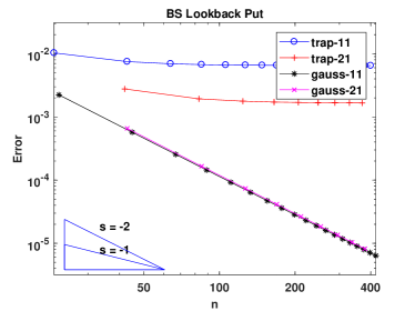
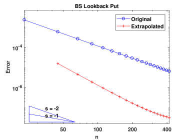
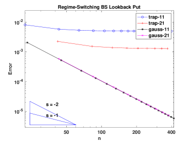
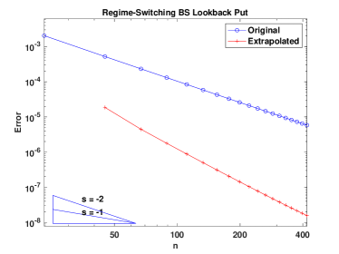
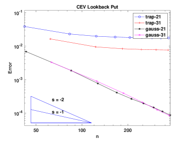
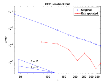
Figure 1: The convergence of a floating strike lookback put option in the Black-Scholes model, the regime-switching Black-Scholes model and the CEV model. Here “trap-11” means the trapezoidal rule with $11$ points is used in (17) and “gauss-11” means the Gauss quadrature rule with $11$ terms is applied. “trap-21”, “trap-31”, “gauss-21” and “gauss-31” have similar meanings. On the right panel, the “Original” is the corresponding line of “gauss-11” on the left panel except the CEV model for which “gauss-21” is used. The “Extrapolation” line is obtained from “Original” by applying Richardson extrapolation based on second order convergence.

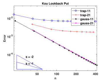
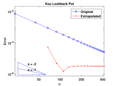
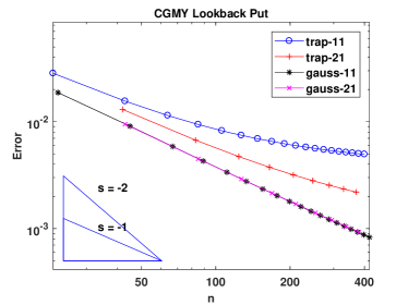
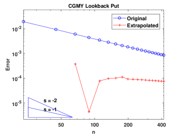
Figure 2: The convergence of a floating strike lookback put option in the Kou model and the CGMY model with extrapolation results. Here “trap-11”, “gauss-11”, “trap-21” and “gauss-21” have the same meaning as in Figure 1. On the right panel, the “Original” is the corresponding line of “gauss-11” on the left panel. The “Extrapolation” line is obtained from “Original” by three-point extrapolation.

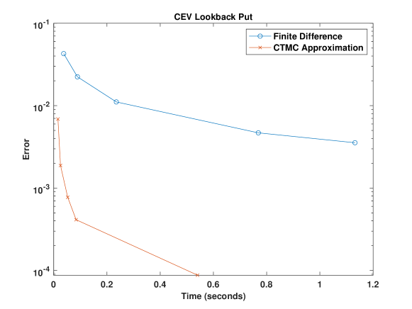
Figure 3: A comparison between a finite difference scheme and our algorithm for the floating strike lookback put option under the CEV model. The benchmark price is obtained from Davydov and Linetsky (2001).

5 Conclusion

This paper develops a general approach to price lookback options by combining numerical quadrature with continuous-time Markov chain approximation. CTMC approximation has proved to be a computationally efficient tool for pricing various types of options. Our analysis reveals that directly using CTMC approximation to price lookbacks is not efficient enough. However, when it is combined with an efficient numerical quadrature such as Gauss quadrature, we can obtain a very efficient algorithm. Our method is applicable to a range of commonly used Markov models, including 1D time-homogeneous and time-inhomogeneous Markov processes, regime-switching models and stochastic local volatility models.

The lookback options considered in the paper do not allow early exercise. The pricing of American-style floating-strike lookback puts is treated in Zhang et al. (2021), where we convert it to the pricing of American drawdown options after a measure change. The problem can be efficiently solved by combining CTMC approximation with an efficient solver for variational inequalities. The other types of American-style lookback options can be priced using similar ideas. In future research, we can consider extending our approach to deal with other types of nonstandard lookback options (see Fusai (2010)) as well as two-asset double lookback options proposed in He et al. (1998).

References

- Aitsahlia and Lai (1998) Aitsahlia, F. and T. Lai (1998). Random walk duality and the valuation of discrete lookback options. Applied Mathematical Finance 5(3-4), 227–240.
- Andricopoulos et al. (2003) Andricopoulos, A. D., M. Widdicks, P. W. Duck, and D. P. Newton (2003). Universal option valuation using quadrature methods. Journal of Financial Economics 67(3), 447–471.
- Andricopoulos et al. (2007) Andricopoulos, A. D., M. Widdicks, D. P. Newton, and P. W. Duck (2007). Extending quadrature methods to value multi-asset and complex path dependent options. Journal of Financial Economics 83(2), 471–499.
- Atkinson and Fusai (2007) Atkinson, C. and G. Fusai (2007). Discrete extrema of Brownian motion and pricing of exotic options. Journal of Computational Finance 10(3), 1.
- Babbs (2000) Babbs, S. (2000). Binomial valuation of lookback options. Journal of Economic Dynamics and Control 24(11-12), 1499–1525.
- Boyarchenko and Levendorskiǐ (2013) Boyarchenko, S. and S. Levendorskiǐ (2013). Efficient Laplace inversion, Wiener-Hopf factorization and pricing lookbacks. International Journal of Theoretical and Applied Finance 16(03), 1–40.
- Boyle and Tian (1999) Boyle, P. and W. Tian (1999). Pricing lookback and barrier options under the CEV process. Journal of Financial and Quantitative Analysis 34(2), 241–264.
- Broadie et al. (1999) Broadie, M., P. Glasserman, and S. Kou (1999). Connecting discrete and continuous path-dependent options. Finance and Stochastics 3(1), 55–82.
- Broadie and Yamamoto (2005) Broadie, M. and Y. Yamamoto (2005). A double-exponential fast Gauss transform algorithm for pricing discrete path-dependent options. Operations Research 53(5), 764–779.
- Cai et al. (2019) Cai, N., S. Kou, and Y. Song (2019). A unified framework for computing regime-switching models. Available at SSRN 3310365.
- Cai et al. (2015) Cai, N., Y. Song, and S. Kou (2015). A general framework for pricing Asian options under Markov processes. Operations Research 63(3), 540–554.
- Carr et al. (2002) Carr, P., H. Geman, D. B. Madan, and M. Yor (2002). The fine structure of asset returns: an empirical investigation. The Journal of Business 75(2), 305–332.
- Cheuk and Vorst (1997) Cheuk, T. H. and T. Vorst (1997). Currency lookback options and observation frequency: a binomial approach. Journal of International Money and Finance: theoretical and empirical research in international economics and finance 16, 173–187.
- Conze (1991) Conze, A. (1991). Path dependent options: The case of lookback options. The Journal of Finance 46(5), 1893–1907.
- Cui et al. (2018) Cui, Z., J. L. Kirkby, and D. Nguyen (2018). A general valuation framework for SABR and stochastic local volatility models. SIAM Journal on Financial Mathematics 9(2), 520–563.
- Cui et al. (2018) Cui, Z., C. Lee, and Y. Liu (2018). Single-transform formulas for pricing Asian options in a general approximation framework under Markov processes. European Journal of Operational Research 266(3), 1134–1139.
- Cui and Taylor (2021) Cui, Z. and S. Taylor (2021). Pricing discretely monitored barrier options under Markov processes through Markov chain approximation. The Journal of Derivatives 28(3), 8–33.
- Dai (2000) Dai, M. (2000). A modified binomial tree method for currency lookback options. Acta Mathematica Sinica 16(3), 445–454.
- Davydov and Linetsky (2001) Davydov, D. and V. Linetsky (2001). Pricing and hedging path-dependent options under the CEV process. Management Science 47(7), 949–965.
- Eriksson and Pistorius (2015) Eriksson, B. and M. R. Pistorius (2015). American option valuation under continuous-time Markov chains. Advances in Applied Probability 47(2), 378–401.
- Feng and Linetsky (2009) Feng, L. and V. Linetsky (2009). Computing exponential moments of the discrete maximum of a Lévy process and lookback options. Finance and Stochastics 13(4), 501–529.
- Forsyth et al. (1999) Forsyth, P., K. Vetzal, and R. Zvan (1999). A finite element approach to the pricing of discrete lookbacks with stochastic volatility. Applied Mathematical Finance 6(2), 87–106.
- Fusai (2010) Fusai, G. (2010). Lookback options. Encyclopedia of Quantitative Finance.
- Fusai et al. (2016) Fusai, G., G. Germano, and D. Marazzina (2016). Spitzer identity, wiener-hopf factorization and pricing of discretely monitored exotic options. European Journal of Operational Research 251(1), 124–134.
- Fusai and Recchioni (2007) Fusai, G. and M. C. Recchioni (2007). Analysis of quadrature methods for pricing discrete barrier options. Journal of Economic Dynamics and Control 31(3), 826–860.
- Fusai and Roncoroni (2008) Fusai, G. and A. Roncoroni (2008). Implementing Models in Quantitative Finance: Methods and Cases. Springer.
- Glasserman (2013) Glasserman, P. (2013). Monte Carlo Methods in Financial Engineering. Springer.
- Goldman et al. (1979) Goldman, M. B., H. B. Sosin, and M. A. Gatto (1979). Path dependent options: “buy at the low, sell at the high”. The Journal of Finance 34(5), 1111–1127.
- Green et al. (2010) Green, R., G. Fusai, and I. D. Abrahams (2010). The Wiener–Hopf technique and discretely monitored path-dependent option pricing. Mathematical Finance 20(2), 259–288.
- He et al. (1998) He, H., W. P. Keirstead, and J. Rebholz (1998). Double lookbacks. Mathematical Finance 8(3), 201–228.
- Higham (2005) Higham, N. J. (2005). The scaling and squaring method for the matrix exponential revisited. SIAM Journal on Matrix Analysis and Applications 26(4), 1179–1193.
- Karatzas and Shreve (2012) Karatzas, I. and S. Shreve (2012). Brownian Motion and Stochastic Calculus. Springer.
- Kou (2002) Kou, S. (2002). A jump-diffusion model for option pricing. Management Science 48(8), 1086–1101.
- Li and Zhang (2016) Li, L. and G. Zhang (2016). Option pricing in some non-Lévy jump models. SIAM Journal on Scientific Computing 38(4), B539–B569.
- Li and Zhang (2018) Li, L. and G. Zhang (2018). Error analysis of finite difference and Markov chain approximations for option pricing. Mathematical Finance 28(3), 877–919.
- Linetsky (2004) Linetsky, V. (2004). Lookback options and diffusion hitting times: A spectral expansion approach. Finance and Stochastics 8(3), 373–398.
- Meier et al. (2021) Meier, C., L. Li, and G. Zhang (2021). Markov chain approximation of one-dimensional sticky diffusions. Advances in Applied Probability 53(2), 335–369.
- Mijatović and Pistorius (2010) Mijatović, A. and M. R. Pistorius (2010). Continuously monitored barrier options under Markov processes: Unabridged version with Matlab code. Available at SSRN 1462822.
- Mijatović and Pistorius (2013) Mijatović, A. and M. R. Pistorius (2013). Continuously monitored barrier options under Markov processes. Mathematical Finance 23(1), 1–38.
- Petrella and Kou (2004) Petrella, G. and S. Kou (2004). Numerical pricing of discrete barrier and lookback options via Laplace transforms. Journal of Computational Finance 8, 1–38.
- Press et al. (2007) Press, W. H., S. A. Teukolsky, W. T. Vetterling, and B. P. Flannery (2007). Numerical Recipes: The Art of Scientific Computing (3rd ed.). Cambridge University Press.
- Serfozo (2009) Serfozo, R. (2009). Basics of Applied Stochastic Processes. Springer.
- Song et al. (2018) Song, Y., N. Cai, and S. Kou (2018). Computable error bounds of Laplace inversion for pricing Asian options. INFORMS Journal on Computing 30(4), 634–645.
- Tse et al. (2001) Tse, W. M., L. K. Li, and K. W. Ng (2001). Pricing discrete barrier and hindsight options with the tridiagonal probability algorithm. Management Science 47(3), 383–393.
- Zhang and Li (2019) Zhang, G. and L. Li (2019). Analysis of Markov chain approximation for option pricing and hedging: Grid design and convergence behavior. Operations Research 67(2), 407–427.
- Zhang and Li (2021a) Zhang, G. and L. Li (2021a). Analysis of Markov chain approximation for diffusion models with non-smooth coefficients. Available at SSRN 3387751.
- Zhang and Li (2021b) Zhang, G. and L. Li (2021b). A general approach for Parisian stopping times under Markov processes. arXiv preprint arXiv:2107.06605.
- Zhang and Li (2021c) Zhang, G. and L. Li (2021c). A general method for analysis and valuation of drawdown risk under Markov models. Available at SSRN 3817591.
- Zhang et al. (2021) Zhang, X., L. Li, and G. Zhang (2021). Pricing American drawdown options under Markov models. European Journal of Operational Research 293(3), 1188–1205.