Orientation of Fitch Graphs and Detection of Horizontal Gene Transfer in Gene Trees

Abstract

Horizontal gene transfer events partition a gene tree $T$ and thus, its leaf set into subsets of genes whose evolutionary history is described by speciation and duplication events alone. Indirect phylogenetic methods can be used to infer such partitions $\mathcal{P}$ from sequence similarity or evolutionary distances without any a priory knowledge about the underlying tree $T$. In this contribution, we assume that such a partition $\mathcal{P}$ of a set of genes $X$ is given and that, independently, an estimate $T$ of the original gene tree on $X$ has been derived. We then ask to what extent $T$ and the xenology information, i.e., $\mathcal{P}$ can be combined to determine the horizontal transfer edges in $T$. We show that for each pair of genes $x$ and $y$ with $x,y$ being in different parts of $\mathcal{P}$, it can be decided whether there always exists or never exists a horizontal gene transfer in $T$ along the path connecting $y$ and the most recent common ancestor of $x$ and $y$. This problem is equivalent to determining the presence or absence of the directed edge $(x,y)$ in so-called Fitch graphs; a more fine-grained version of graphs that represent the dependencies between the sets in $\mathcal{P}$. We then consider the generalization to insufficiently resolved gene trees and show that analogous results can be obtained. We show that the classification of $(x,y)$ can be computed in constant time after linear-time preprocessing. Using simulated gene family histories, we observe empirically that the vast majority of horizontal transfer edges in the gene tree $T$ can be recovered unambiguously.

Keywords: gene families, xenology, horizontal gene transfer, Fitch graph, partition, linear-time algorithm

1 Introduction

Gene family histories (GFHs) play an important role for the understanding of innovations in evolutionary biology. A GFH describes the changes in the set of related genes along the evolutionary history of a set of species of interest. Mathematically, this amounts to the “reconciliation”, i.e., the embedding of a gene tree $T$ into a species tree $S$, such that the nodes of $T$ describing gene duplication and horizontal gene transfer (HGT) events are mapped into the edges of $S$, see e.g. (Hellmuth and Wieseke, 2016; Setubal and Stadler, 2018; Altenhoff et al., 2019) and the references therein. Each transfer edge of $T$ must then be mapped in a way such that its endpoints are mapped to distinct lineages in $S$. In practice, the accurate inference in particular of the gene tree $T$ from sequence data, however, is a difficult problem plagued by biases and technical artifacts associated with the necessity to extract additive dissimilarities between genes.

An alternative – combinatorial – approach avoids the requirement of additive distances and instead uses only qualitative comparisons of pairwise distances (Hellmuth et al., 2015). In particular, two types of information have turned out to be useful: the best matches of a gene in the genome of a different species (Geiß et al., 2019), and the fact that the last common ancestor of a pair of genes is younger than the last common ancestor of the species in which they reside (Schaller et al., 2021b). Both types of data yield vertex-colored graphs whose vertices represent the genes with colors identifying the species in which they reside. The best match graphs (BMG) (Geiß et al., 2019) are directed. In contrast, the later-divergence-time (LDT) graphs are undirected and capture HGT events. More precisely, LDTs can be used to find a partition $\mathcal{P}$ of the set of genes such that within each subset the genes that are not separated by a HGT event since their last common ancestor, while HGT events separate distinct subsets of this partition. The best match graph, on the other hand, can be used to infer a minor of the gene tree $T$, i.e., a not necessarily fully resolved version of $T$. Alternatively, estimated orthology graphs, which are equivalent to cographs or, more general, to symbolic ultrametrics (Böcker and Dress, 1998; Hellmuth et al., 2013), can be used to infer a minor of $T$ (Hellmuth et al., 2015). It is of practical interest, therefore, to identify the edges of $T$ that correspond to HGT events (Jones et al., 2017; Schaller et al., 2021b). Here we ask to what extent this is possible based on a given tree $T$ and a given partition $\mathcal{P}$ of the leaf set of $T$ into HGT-free subsets.

The Fitch graph of a GFH also has the genes as vertices and features a directed edge from gene $x$ to gene $y$ whenever a horizontal transfer event was present between $y$ and the last common ancestor of $x$ and $y$ (Geiß et al., 2018). Consequently, $x$ and $y$ belong to different sets of $\mathcal{P}$. The symmetrized Fitch graph (Hellmuth et al., 2018) thus is the complete multipartite graph that has the sets of $\mathcal{P}$ as its maximal independent sets. It is of practical interest, therefore, to investigate to what extent the partition $\mathcal{P}$ already identifies the placement of the HGT events in the tree $T$. In related work, we recently characterized under which conditions an orthology graph, i.e., a symbolic ultrametric, and a Fitch graph are consistent in the sense that they can be explained by a common vertex- and edge-annotated gene tree $T$ (Hellmuth et al., 2021a). Using this information, a GFH, i.e., a species tree $S$ together with a time-consistent reconciliation map between the annotated gene tree $T$ and $S$, can then be determined in polynomial time, provided it exists (Hellmuth, 2017; Nøjgaard et al., 2018; Lafond and Hellmuth, 2020). From a practical point of view, however, this result is of limited use since so far there is no efficient means of inferring the directed Fitch graph directly from data, while its symmetrized counterpart is accessible from empirical data (Schaller et al., 2021b). This prompts us to ask to what extent the compatibility of $T$ and $\mathcal{P}$ determines the orientation of the edges in the Fitch graph. As we shall see below, the placement of HGT edges in $T$ and the orientation of the edges of the Fitch graph are very closely related. After introducing the necessary notation in Section 2, we give an overview of the concepts and results in Section 3.

2 Preliminaries

We denote the power set of a set $L$ by $2^{L}$. A set system $\mathcal{P}\subseteq 2^{L}$ is a partition of $L$ if (P0) $\emptyset\notin\mathcal{P}$, (P1) $\bigcup_{\_}{A\in\mathcal{P}}A=L$, and (P2) if $A,B\in\mathcal{P}$ and $A\cap B\neq\emptyset$ then $A=B$. We write $(x,y)$ for ordered pairs and $\{x,y\}$ for unordered pairs of elements $x,y\in L$. For a graph $G=(V,E)$, we write $V(G)=V$ and $E(G)=E$ for its vertex and edge set, respectively. Edges are denoted by $(x,y)$ in directed graphs and $\{x,y\}$ in undirected graphs.

We consider rooted phylogenetic trees $T$ with root $\rho_{\_}T$, vertex set $V(T)$, edge set $E(T)$, and leaf set $L=L(T)\subseteq V(T)$. The set of inner vertices is $V^{0}(T)\coloneqq V(T)\setminus L$ the set of vertices that are distinct from the leaves. For any two vertices $x,y\in V(T)$, the path $P_{\_}{x,y}$ connecting $x$ and $y$ in $T$ is a uniquely defined subgraph of $T$. The ancestor relation $\preceq_{\_}T$ on $V(T)$ is given by $v\preceq_{\_}Tu$ if and only if $u$ lies on the unique path from $v$ to the root. We write $v\prec_{\_}Tu$ for $v\preceq_{\_}Tu$ and $v\neq u$. To distinguish tree edges from edges of graphs defined on $L$, we write $uv$ instead of $\{u,v\}$ or $(u,v)$ and use the convention that the notation $uv$ for edges in $T$ implies $v\prec_{\_}Tu$, i.e., $v$ is a child of $u$ and $u$ is the unique parent of $v$, in symbols $u=\operatorname{par}_{\_}T(v)$. The set of children of a vertex $u$ is denoted by $\operatorname{child}_{\_}T(u)$. Two vertices $u,v\in V(T)$ are comparable if $v\preceq_{\_}Tu$ or $u\preceq_{\_}Tv$. The last common ancestor of a set $A\subseteq V(T)$, denoted by $\operatorname{lca}_{\_}T(A)$, is the unique $\preceq_{\_}T$-minimal element in $V(T)$ that satisfies $v\preceq_{\_}T\operatorname{lca}_{\_}T(A)$ for all $v\in A$. For simplicity, we often write $\operatorname{lca}_{\_}T(x,y)$ instead of $\operatorname{lca}_{\_}T(\{x,y\})$. We will often make use of the observation that $\operatorname{lca}_{\_}{T}(A\cup B)=\operatorname{lca}_{\_}{T}(\operatorname{lca}_{\_}{T}(A),\operatorname{lca}_{\_}{T}(B))$ for two subsets $A,B\subseteq V(T)$. For $u\in V(T)$, we denote by $T(u)$ the subtree of $T$ induced by $\{v\in V(T)\mid v\preceq_{\_}Tu\}$ with root $u$. If there is no risk of confusion and the context is clear, we will omit the explicit reference to $T$, that is, we omit the subscript “${}_{\_}T$”.

We note that the trees considered here are slightly less general than the so-called $X$-trees commonly used in mathematical phylogenetics (Semple and Steel, 2003). In an $X$-tree, a set of “taxa” $X$ is mapped (not necessarily injectively) to the vertex set $V(T)$ of a tree $T$. Here we consider phylogenetic trees in which distinct taxa are represented by distinct leaves of $T$. That is, our phylogenetic trees are equivalent to $X$-trees in which the taxa set $X$ is mapped bijectively to $L(T)$.

A hierarchy on $L$ is a system $\mathcal{H}\subset 2^{L}$ of non-empty sets such that (i) $A\cap B\in\{\emptyset,A,B\}$ for all $A,B\in\mathcal{H}$, (ii) $L\in\mathcal{H}$, and (iii) $\{x\}\in\mathcal{H}$ for all $x\in L$.

Proposition 1.

(Semple and Steel, 2003)  Let $\mathcal{H}$ be a collection of non-empty subsets of $X$. Then, $\mathcal{H}$ is a hierarchy on $X$ if and only if there is a rooted phylogenetic tree $T$ on $X$ with $\mathcal{H}=\{L(T(v))\mid c\in V(T)\}$.

As a consequence, there is a 1-to-1 correspondence between phylogenetic trees with leaf set $L$ and hierarchies on $L$ by virtue of $A\in\mathcal{H}$ if and only if $A=L(T(v))$ for $v=\operatorname{lca}_{\_}T(A)$. We often write $\mathcal{H}(T)\coloneqq\{L(T(v))\mid v\in V(T)\}$ for the hierarchy that is associated by $T$ and refer to the sets $L(T(v))$ as clusters in $T$. In particular, it holds that $L(T(v))\subseteq L(T(u))$ if and only if $v\preceq_{\_}Tu$ for all $u,v\in V(T)$. The map $\operatorname{cl}_{\_}{T}\colon 2^{L}\to 2^{L}$ defined by $\operatorname{cl}_{\_}{T}(A)\coloneqq L(T(\operatorname{lca}_{\_}T(A)))$, which assigns to $A$ the unique inclusion-minimal superset in $\mathcal{H}$, is the canonical closure on $\mathcal{H}$, as it coincides for hierarchies with the intersection of all $B\in\mathcal{H}$ with $A\subseteq B$. A tree $T^{\prime}$ is a refinement of a tree $T$, if $\mathcal{H}(T)\subseteq\mathcal{H}(T^{\prime})$. Equivalently, $T^{\prime}$ is a refinement of $T$, if $T$ can be obtained from $T^{\prime}$ by a series of edge-contractions.

Throughout, we will assume that we are given a pair of a tree $T$ with leaf set $L$ (or its associated hierarchy $\mathcal{H}$) and a partition $\mathcal{P}$ of $L$.

3 Main Ideas and Results

In the formal representations of gene family histories, an HGT event is a property of an edge $uv$ in the gene tree $T$. More precisely, $uv$ is an HGT edge if $u$ and $v$ are mapped into the species tree $S$ in such a way that that their images are not in an ancestor-descendant relationship, see Fig. 1 for examples. Here, we will not consider GFHs explicitly. Instead, we focus only on gene trees and HGT events. In (Geiß et al., 2018; Hellmuth et al., 2018) the latter are modeled as an edge labeling $\lambda:E(T)\to\{0,1\}$. Here, it will be more convenient to think of HGTs as the subset $H\subseteq E(T)$ of edges in the gene tree $T$ with $e\in H$ if and only if $\lambda(e)=1$.

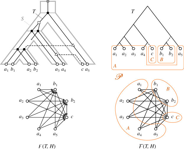
Figure 1: A gene family history (GFH) (upper left) consisting of a gene tree $T$ embedded into a species tree $S$. Apart from speciations ($\newmoon$), events such as gene duplications ($\square$), losses ($\perp$), and horizontal gene transfers ($\triangle$ and dashed lines) shape the history of a gene family. The gene tree $T$ is shown again in the upper right panel, without the event labels at the inner vertices; the set $H\subseteq E(T)$ of HGT edges is again displayed by dashed lines. Removal of $H$ induces the partition $\mathcal{P}\coloneqq\mathfrak{P}(T,H)=\{A,B,C\}$ of $L$. The directed and symmetrized Fitch graphs, $\digamma(T,H)$ and $\overline{\digamma}(T,H)$, resp., are shown in the two lower panels. The set of inclusion-maximal independent sets of $\overline{\digamma}(T,H)$ coincides with $\mathcal{P}$.

Given $T$ and $H\subseteq E(T)$, we write $T-H\coloneqq(V(T),E(T)\setminus H)$ for the forest obtained by removing the edges $H$ in $T$. Moreover, $\mathfrak{P}(T,H)$ is the partition of $L$ induced by the connected components of $T-H$. Two genes $x,y\in L$ are called xenologs if their history since their last common ancestor involves a horizontal transfer (Fitch, 2000), i.e., if the path connecting $x$ and $y$ in $T$ contains a transfer edge $e\in H$. Hence, $x$ and $y$ are xenologs if and only if they are located in distinct sets of $\mathfrak{P}(T,H)$.

Xenology has been modeled both with the help of directed and undirected graphs. The (directed) Fitch graph $\digamma\coloneqq\digamma(T,H)$ has vertex set $V(\digamma)=L(T)$ and a directed arc $(x,y)\in E(\digamma)$ if and only if the path $P_{\_}{\operatorname{lca}(x,y),y}$ from $\operatorname{lca}_{\_}T(x,y)$ to $y$ contains an edge $e\in H$ (Geiß et al., 2018). A digraph $G=(V,E)$ is a Fitch graph if there is a tree $T$ and a subset $H\subseteq E(T)$ such that $G=\digamma(T,H)$. The symmetrized Fitch graph $\overline{\digamma}\coloneqq\overline{\digamma}(T,H)$ has an undirected edge $\{x,y\}\in E(\overline{\digamma})$ whenever $(x,y)\in E(\digamma)$ or $(y,x)\in E(\digamma)$ (Hellmuth et al., 2018). Symmetrized Fitch graphs are complete multipartite graphs. More precisely, the inclusion-maximal independent sets of $\overline{\digamma}$ form a unique partition $\mathcal{P}$ of $V(G)$ such that $\{x,y\}\in E(\overline{\digamma})$ if and only if $x$ and $y$ are in distinct sets of $\mathcal{P}$. The partition $\mathfrak{P}(T,H)$ therefore coincides with the set $\mathcal{P}$ of inclusion-maximal independent sets of $\overline{\digamma}(T,H)$, see Fig. 1.

Due to the one-to-one correspondence between symmetrized Fitch graphs and partitions, it suffices to consider compatibility of trees and partitions.

Definition 1.

Let $\mathcal{P}$ be a partition of $L$ and let $T$ be a tree with leaf set $L$. Then $\mathcal{P}$ and $T$ (or equivalently its associated hierarchy $\mathcal{H}$) are compatible if there is a set $H\subseteq E(T)$ such that $\mathcal{P}=\mathfrak{P}(T,H)$.
In this case, we call $H$ a separating set (for $(T,\mathcal{P})$) and say that $T$ (and, equivalently, $\mathcal{H}$) and $\mathcal{P}$ are $H$-compatible.

Equivalently, one may define $T$ and $\overline{\digamma}$ as compatible if $\overline{\digamma}=\overline{\digamma}(T,H)$ for some subset $H\subseteq E(T)$. Hellmuth et al. (2021b, Thm. 4.5) showed that $T$ and $\mathcal{P}$ are compatible if and only if, for all $A,B\in\mathcal{P}$, it holds (i) $\operatorname{cl}_{\_}{T}(A)$ is a union of sets of $\mathcal{P}$ and (ii) $\operatorname{cl}_{\_}{T}(A)=\operatorname{cl}_{\_}{T}(B)$ implies $A=B$.

Since $\overline{\digamma}(T,H)$ is a complete multipartite graph whose independent sets are formed precisely by the vertices of the parts in $\mathcal{P}$, the quotient graph $\overline{\digamma}(T,H)/\mathcal{P}\simeq K_{\_}{|\mathcal{P}|}$ is a complete graph on $|\mathcal{P}|$ vertices.

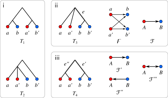
Figure 2: Examples of trees that are (in)compatible with the partition $\mathcal{P}=\{A\coloneqq\{a,a^{\prime}\},B\coloneqq\{b,b^{\prime}\}\}$. (i) Both $T_{\_}1$ and $T_{\_}2$ are incompatible with $\mathcal{P}$ since every edge in $T$ lies on a path that connects elements from $A$ or $B$. (ii) The tree $T_{\_}3$ is compatible with $\mathcal{P}$ with a unique choice for the separating set $H=\{e\}$. Hence, the only possible Fitch graph is $\digamma=\digamma(T,H)$ with corresponding Fitch quotient graph $\mathscr{F}=\digamma/\mathcal{P}$. (iii) The tree $T_{\_}4$ is compatible with $\mathcal{P}$ and admits three valid choices for the separating set $H^{\prime}=\{e^{\prime}\}$, $H^{\prime\prime}=\{e^{\prime\prime}\}$, and $H^{\prime\prime\prime}=\{e^{\prime},e^{\prime\prime}\}$ yielding Fitch quotient graphs $\mathscr{F}^{\prime}$, $\mathscr{F}^{\prime\prime}$, and $\mathscr{F}^{\prime\prime\prime}$, respectively.

We will show that the directed quotient digraph $\mathscr{F}(T,H)\coloneqq\digamma(T,H)/\mathcal{P}$ completely determines the edges of $\digamma(T,H)$ such that $(x,y)\in E(\digamma(T,H))$ if and only if $x\in A$, $y\in B$ and $(A,B)\in E(\mathscr{F}(T,H))$, see Lemma 7 and Cor. 2 below. Therefore, it suffices to consider $\mathscr{F}(T,H)$, which we will occasionally denote by $\mathscr{F}$ for brevity. Since its symmetrized version is a complete graph, we have $(A,B)\in E(\mathscr{F}(T,H))$ or $(B,A)\in E(\mathscr{F}(T,H))$ for any two distinct $A,B\in\mathcal{P}$. An example for a Fitch graph $\digamma$ and its corresponding quotient graph $\mathscr{F}$ is shown in Fig. 2(ii).

Definition 2.

A graph $G$ is a Fitch quotient graph for $(T,\mathcal{P})$ if there is $H\subseteq E(T)$ such that $G=\mathscr{F}(T,H)$.

Below, we compile the notation for the different variants of Fitch graphs and associated constructs appearing throughout this contribution:

$\digamma\coloneqq\digamma(T,H)$	…	(directed) Fitch graph
$\mathscr{F}\coloneqq\mathscr{F}(T,H)\coloneqq\digamma(T,H)/\mathcal{P}$	…	(directed) Fitch quotient graph
$\overline{\digamma}\coloneqq\overline{\digamma}(T,H)$	…	symmetrized Fitch graph
$\overline{\digamma}(T,H)/\mathcal{P}\simeq K_{\_}{|\mathcal{P}|}$	…	quotient of symmetrized Fitch graph
$\mathfrak{P}(T,H)$	…	partition of $L$ based on $T-H$
$\mathcal{P}$	…	arbitrary partition of $L$
$\mathcal{H}$	…	arbitrary hierarchy on $L$

In Section 4, we will be concerned with the question to what extent the separating set $H$ is already determined by $T$ and $\mathcal{P}$.

Definition 3.

An edge $h\in E(T)$ is an essential separating edge if $h\in H$ for all $H$ satisfying $\mathfrak{P}(T,H)=\mathcal{P}$, a forbidden separating edge if $h\in H$ for all $H$ satisfying $\mathfrak{P}(T,H)=\mathcal{P}$, and an ambiguous separating edge otherwise.

Consider the examples in Fig. 2. The edge $e$ in the tree $T_{\_}3$ is clearly an essential separating edge since it is the only edge that separates the set $A,B\in\mathcal{P}$ without at the same time separating elements from $A$ or $B$. In contrast, the edges on the path connecting $a$ and $a^{\prime}$ (or $b$ and $b^{\prime}$) are clearly forbidden separating edges. Finally, the edges $e^{\prime}$ and $e^{\prime\prime}$ in $T_{\_}4$ are ambiguous separating edges since $H^{\prime}=\{e^{\prime}\}$ and $H^{\prime\prime}=\{e^{\prime\prime}\}$ are both valid choices for the separating set. In order to classify tree edges as (un)ambiguously present or absent in the separating set, we will use the following vertex coloring, which is well-defined for a compatible pair $(T,\mathcal{P})$ as a consequence of Lemma 1 below.

Definition 4.

Let $T$ and $\mathcal{P}$ be compatible. Then, $\varpi\colon V(T)\to\mathcal{P}\cup\{\emptyset\}$ is defined by putting, for all $v\in V(T)$, $\varpi(v)\coloneqq A$ if there are $x,y\in A$ such that $v$ lies along the path connecting $x$ and $y$ in $T$. If no such path exists, then $\varpi(v)\coloneqq\emptyset$.

We will refer to $u\in V(T)$ as a colored vertex if $\varpi(u)\neq\emptyset$. For all $x,y\in A$ and all $A\in\mathcal{P}$ we have, by construction, $\varpi(x)=\varpi(y)=A$, $\varpi(\operatorname{lca}(x,y))=A$, and $\varpi(\operatorname{lca}(A))=A$. The main result of Section 4 characterizes the classification of tree edges in Def. 3 in terms of the vertex coloring $\varpi$:

Main Result A (Thm. 1). An edge $vw\in E(T)$ is an essential separating edge if and only if $\emptyset\neq\varpi(v)\neq\varpi(w)\neq\emptyset$; a forbidden separating edge if and only if $\emptyset\neq\varpi(v)=\varpi(w)$; and an ambiguous separating edge otherwise.

A particular separating set $H$ for a compatible pair $(T,\mathcal{P})$ also determines whether or not a pair $(A,B)\in\mathcal{P}\times\mathcal{P}$ is an edge of $\mathscr{F}(T,H)$. Naturally, we ask to what extent the presence or absence of an edge $(A,B)$ is already determined by $T$ and $\mathcal{P}$. The examples in Fig. 2(ii) and (iii), respectively, show that, for a given compatible pair of a partition $\mathcal{P}$ and a tree $T$, edges in the Fitch quotient graph may be unambiguously present (or absent) or only present for specific choices of the separating set.

Definition 5.

Let $T$ and $\mathcal{P}$ be compatible and let $A,B\in\mathcal{P}$ be distinct. Then $(A,B)$ is essential if $(A,B)\in E(\mathscr{F}(T,H))$ for all separating sets $H$ of $(T,\mathcal{P})$, and $(A,B)$ is forbidden if $(A,B)\notin E(\mathscr{F}(T,H))$ for every separating set $H$ of $(T,\mathcal{P})$. Otherwise, we say that $(A,B)$ is ambiguous.

In particular, if $(A,B)$ is ambiguous, then there are choices of separating sets $H_{\_}1$ and $H_{\_}2$ for $(T,\mathcal{P})$ such that $(A,B)\in E(\mathscr{F}(T,H_{\_}1))$ and $(A,B)\notin E(\mathscr{F}(T,H_{\_}2))$.

In Section 5, we turn to characterizing essential and forbidden edges in the Fitch quotient graphs for compatible $T$ and $\mathcal{P}$. The main result of this section provides a complete characterization of $(A,B)$ as essential, forbidden, or ambiguous in terms of the vertex coloring $\varpi$ of $T$ and the relative positions of the last common ancestors of $A,B\in\mathcal{P}$, and $A\cup B$ in $T$. More precisely, we will show:

Main Result B (Thm. 2). $(A,B)$ is essential if and only if there is a colored vertex $v\in V^{0}(T)$ such that $\operatorname{lca}(B)\prec v\preceq\operatorname{lca}(A\cup B)$; $(A,B)$ is forbidden if and only if $\operatorname{lca}(A)\prec\operatorname{lca}(B)$; and $(A,B)$ is ambiguous otherwise.

Furthermore, we describe an $O(|L|+|\mathcal{P}|^{2})$ algorithm that computes this classification explicitly for all pairs $A,B\in\mathcal{P}$, see Cor. 5.

So far, we have assumed that $T$ comprises all (not necessarily binary) branching events that occurred in the evolution of the gene family. However, poorly supported edges are often contracted in phylogenetic reconstructions. Combinatorial approaches for gene tree reconstruction also typically only infer a minor of the gene tree $T$. It is therefore of practical interest to consider also possible refinements $T^{\prime}$ of $T$. More precisely, we ask in Section 6 whether there are arcs $(x,y)$ that are present (or absent) in the Fitch graph $\digamma(T^{\prime},H)$ for every refinement $T^{\prime}$ of $T$ that is compatible with $\mathcal{P}$ and every separating set $H$ for $(T^{\prime},\mathcal{P})$. It again suffices to consider the Fitch quotient graphs (cf. Lemma 7 and Cor. 2).

Definition 6.

A tree $T$ with leaf set $L$ is refinement-compatible (r-compatible for short) with a partition $\mathcal{P}$ of $L$ if there is a refinement $T^{\prime}$ of $T$ that is compatible with $\mathcal{P}$.

Note that a tree $T$ can be r-compatible with $\mathcal{P}$ although $T$ and $\mathcal{P}$ are not compatible, see Fig. 3(i) for an example. Answering the question whether $T$ is r-compatible with $\mathcal{P}$ thus provides additional information about the topology of phylogenetic trees that is implicitly contained in $\mathcal{P}$ or $\overline{\digamma}$. Refinement compatibility was characterized by Hellmuth et al. (2021b) in the following manner:

Proposition 2.

(Hellmuth et al., 2021b, Prop. 7.3 and Thm. 7.5)  Let $T$ be a tree on $L$ and $\mathcal{P}$ be a partition of $L$. Then $T$ and $\mathcal{P}$ are r-compatible if and only if there is no edge $e\in E(T)$ lying on the path from $x$ to $x^{\prime}$ and on the path from $y$ to $y^{\prime}$ such that $x,x^{\prime}\in A$ and $y,y^{\prime}\in B$ for distinct $A,B\in\mathcal{P}$. In the positive case, a compatible refinement $T^{\prime}$ of $T$ can be constructed in $O(|L|)$ operations.

Moreover, Hellmuth et al. (2021b, Prop. 5.1) showed that compatibility of $T$ and $\mathcal{P}$ implies that all refinements of $T$ are again compatible with $\mathcal{P}$. The vertex coloring $\varpi$ is in general not well-defined for an r-compatible pair $(T,\mathcal{P})$ because $T$ does not need to be compatible with $\mathcal{P}$. To see this, consider again Fig. 3(i) and the common parent of vertices $a$, $a^{\prime}$, and $b$ in $T_{\_}1$. This vertex lies on the path connecting $a,a^{\prime}\in A$, as well as on the path connecting $b,b^{\prime}\in B$. Instead of $\varpi$, we therefore consider an edge coloring similar to the one used in (Hellmuth et al., 2021b):

Definition 7.

Let $T$ and $\mathcal{P}$ be r-compatible. Then, $\gamma\colon E(T)\to\mathcal{P}\cup\{\emptyset\}$ is defined by putting, for all $e\in E(T)$, $\gamma(e)\coloneqq A$ if there are $x,y\in A$ such that $e$ lies along the path connecting $x$ and $y$ in $T$, in which case we say that $e$ is colored. If no such path exists, then $\gamma(e)\coloneqq\emptyset$.

The only difference to the edge coloring in (Hellmuth et al., 2021b) is that, as a consequence of Prop. 2, we can directly use the sets $A\in\mathcal{P}$ as “colors” rather than subsets of $2^{\mathcal{P}}$. Generalizing the notion of essential edges in Fitch quotient graphs, we consider pairs $(A,B)$:

Definition 8.

Let $T$ and $\mathcal{P}$ be r-compatible and let $A,B\in\mathcal{P}$ be distinct. We say that $(A,B)$ is r-essential if $(A,B)\in\mathscr{F}(T^{\prime},H)$ for all separating sets $H\subseteq E(T^{\prime})$ of every refinement $T^{\prime}$ of $T$ that is compatible with $\mathcal{P}$. We say that $(A,B)$ is r-forbidden if $(A,B)\notin\mathscr{F}(T^{\prime},H)$ for any separating set $H\subseteq E(T^{\prime})$ of any refinement $T^{\prime}$ of $T$ that is compatible with $\mathcal{P}$. In all other cases, $(A,B)$ is r-ambiguous.

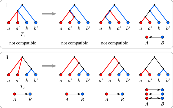
Figure 3: Two trees $T_{\_}1$ and $T_{\_}2$ that are r-compatible with the partition $\mathcal{P}\coloneqq\{A\coloneqq\{a,a^{\prime}\},B\coloneqq\{b,b^{\prime}\}\}$. Edge colors represent $\gamma$ (black edges have color $\emptyset$), except in the first two refinements of $T_{\_}1$ since these are not r-compatible and thus $\gamma$ is not defined. (i) The tree $T_{\_}1$ is not compatible with the partition $\mathcal{P}$. It admits three refinements. Since only the third refinement is compatible with $(B,A)$ being essential and $(A,B)$ being forbidden, we have that $(B,A)$ is r-essential and $(A,B)$ is r-forbidden. (ii) The tree $T_{\_}2$ is compatible with $\mathcal{P}$ with $(A,B)$ being essential and $(B,A)$ being forbidden. Its refinement on the r.h.s. is the example from Fig. 2(iii) admitting multiple choices of the separating set. As a consequence, both $(A,B)$ and $(B,A)$ are r-ambiguous.

If $T$ and $\mathcal{P}$ are already compatible and $(A,B)$ is ambiguous for two sets $A,B\in\mathcal{P}$, then clearly $(A,B)$ is also r-ambiguous since $T$ is a compatible refinement of itself. Analogous statements, however, do not hold for essential and forbidden edges as the example in Fig. 3(ii) shows. By definition, an essential edge $(A,B)$ cannot be r-forbidden, and a forbidden edge $(A,B)$ cannot be r-essential. Therefore, considering refinements cannot decrease the level of ambiguity.

The main result of Section 6 is a characterization of r-essential and r-forbidden pairs $(A,B)$ for a given a tree $T$ and an r-compatible partition $\mathcal{P}$. Similar to our first two main results, the characterization can be expressed in terms of the edge coloring $\gamma$ and the last common ancestors of $A$, $B$, and $u\coloneqq\operatorname{lca}_{\_}T(A\cup B)$ in $T$:

Main Result C (Thm. 3). $(A,B)$ is r-essential if and only if (a) the path $P_{\_}{u,\operatorname{lca}_{\_}{T}(B)}$ contains a colored edge, or (b) $u\neq\rho_{\_}T$ and the path $P_{\_}{u,\operatorname{lca}_{\_}{T}(A)}$ contains a colored edge $e$ with $\gamma(e)=\gamma(\operatorname{par}_{\_}T(u)u)=C\in\mathcal{P}$. $(A,B)$ is r-forbidden if and only if $\operatorname{lca}_{\_}{T}(A)\prec_{\_}T\operatorname{lca}_{\_}{T}(B)=u$ and $\gamma(uv)=B$ for the vertex $v\in\operatorname{child}_{\_}{T}(u)$ satisfying $\operatorname{lca}_{\_}{T}(A)\preceq_{\_}Tv$.

The different situations that make $(A,B)$ r-essential or r-forbidden are illustrated in Fig. 4.

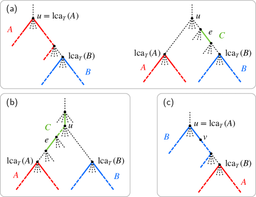
Figure 4: The situations leading to r-essential or r-forbidden pairs $(A,B)$ with $A,B\in\mathcal{P}$ and $u\coloneqq\operatorname{lca}_{\_}{T}(A\cup B)$. Dashed lines indicate paths that may or may not exist. (a) $(A,B)$ is r-essential if the path $P_{\_}{u,\operatorname{lca}_{\_}{T}(B)}$ contains a colored edge. This edge may have color $A$ (left) in which case $u=\operatorname{lca}_{\_}{T}(A)$ or a color $C\in\mathcal{P}\setminus\{A,B\}$ (right). (b) The second possibility leading to $(A,B)$ being r-essential. (c) The situation when $(A,B)$ is r-forbidden.

The characterization also gives rise to an $O(|L|+|\mathcal{P}|^{2})$ algorithm that computes this classification explicitly for all pairs $A,B\in\mathcal{P}$. Implementations of the classification algorithms based on the three main results are applied to simulated GFHs in Section 7 to determine the relative abundances of essential, forbidden, and ambiguous edges in the gene trees and the corresponding Fitch quotient graphs. We will see that ambiguities are surprisingly rare in these evolutionary scenarios.

4 Possible Choices of the Separating Set $H$

In order to understand the ambiguity of edges in the Fitch quotient graph $\mathscr{F}(T,H)$, we first need to understand to what extent the choice of the separating set $H$ is constrained by a given tree $T$ and a partition $\mathcal{P}$. Our starting point is

Proposition 3.

(Hellmuth et al., 2021b, Cor. 7.7)  If $T$ and $\mathcal{P}$ are compatible, then there is a unique inclusion-maximal separating set $H^{*}$ such that $\mathcal{P}=\mathfrak{P}(T,H)$.

By (Hellmuth et al., 2021b, Thm. 7.6), it can be constructed explicitly as the set of all edges $e\in E(T)$ that do not lie along the path connecting a pair of points $x,y\in A$ for any $A\in\mathcal{P}$. Here, we use an even simpler, vertex-centered construction based on the following simple observation:

Lemma 1.

Let $T$ and $\mathcal{P}$ be compatible, $A,A^{\prime}\in\mathcal{P}$ and $v\in V(T)$. If $v$ lies on both the path $P_{\_}{x,y}$ connecting $x,y\in A$ and the $P_{\_}{x^{\prime},y^{\prime}}$ connecting $x^{\prime},y^{\prime}\in A^{\prime}$, then $A=A^{\prime}$.

Proof.

First we note that $E(P_{\_}{x,y})\cap H^{*}=\emptyset$ and $E(P_{\_}{x^{\prime},y^{\prime}})\cap H^{*}=\emptyset$. The union of the path $P_{\_}{x,y}$ and $P_{\_}{x^{\prime},y^{\prime}}$ together form a (non-phylogenetic) sub-tree $T_{\_}4$ of $T$. We therefore have $v\in V(P_{\_}{x,y})\cap V(P_{\_}{x^{\prime},y^{\prime}})=V(P_{\_}{x,x^{\prime}})\cap V(P_{\_}{y,y^{\prime}})$ or $v\in V(P_{\_}{x,y})\cap V(P_{\_}{x^{\prime},y^{\prime}})=V(P_{\_}{x,y^{\prime}})\cap V(P_{\_}{x^{\prime},y})$ and thus $v$ also lies along one of the paths $P_{\_}{x,y^{\prime}}$, $P_{\_}{x,x^{\prime}}$, $P_{\_}{x^{\prime},y}$, or $P_{\_}{y,y^{\prime}}$. Together with $E(T_{\_}4)\cap H^{*}=\emptyset$, this implies $A\cap A^{\prime}\neq\emptyset$ and thus $A=A^{\prime}$ because $\mathcal{P}$ is a partition. ∎

We can therefore uniquely “color” each vertex $v\in V(T)$ by a set $\varpi(v)=A\in\mathcal{P}$ whenever there are $x,y\in A$ such that $v$ lies along the path connecting $x$ and $y$ in $T$; otherwise we set $\varpi(v)=\emptyset$. Hence, the vertex coloring $\varpi\colon V(T)\to\mathcal{P}\cup\{\emptyset\}$ in Def. 4 is well-defined.

Lemma 2.

Let $T$ and $\mathcal{P}$ be $H$-compatible. Then, the map $\varpi$ as well as $\operatorname{lca}(A)$ for all $A\in\mathcal{P}$ can be computed in $O(|L|)$ total time.

Proof.

This proof parallels the construction of an associated edge coloring in the proof of Thm. 7.5 in (Hellmuth et al., 2021b). The LCA data structure described by Bender et al. (2005) enables constant time look-up of $\operatorname{lca}_{\_}T(u,v)$ for any $u,v\in V(T)$ after an $O(|L|)$ preprocessing step. We now show how to compute the map $\varpi$ as well as $\operatorname{lca}(A)$ for all $A\in\mathcal{P}$ in linear total time.

We start by initializing $\varpi(v)=\emptyset$ for all $v\in V(T)$ in $O(|L|)$. We then process every $A=\{x_{\_}1,\dots,x_{\_}k\}\in\mathcal{P}$ as follows. First, we initialize the set of previously visited vertices of $V(T)$ as $\texttt{visited}\leftarrow\emptyset$ and the current last common ancestor as $\texttt{curLCA}\leftarrow x_{\_}1$. The latter will be updated stepwisely such that it equals $\operatorname{lca}_{\_}T(A)$ in the end. To this end, for each leaf $x\in\{x_{\_}2,\dots,x_{\_}k\}$ (if any), we query $\texttt{newLCA}=\operatorname{lca}_{\_}T(x,\texttt{curLCA})$ and move from $x$ upwards along the tree. We set $\varpi(v)=A$ for each vertex $v$ encountered during the traversal, and add $v$ to visited. The traversal stops as soon as $v$ is in visited or equals newLCA. In case we have $\texttt{curLCA}\prec_{\_}T\texttt{newLCA}$, which by definition of newLCA holds if $\texttt{curLCA}\neq\texttt{newLCA}$, we perform the same bottom-up traversal starting from curLCA. As a final step in the processing of $x$, we set $\texttt{curLCA}\leftarrow\texttt{newLCA}$. One easily verifies that, after processing all vertices in $A$, it holds $\operatorname{lca}(A)=\texttt{curLCA}$ and we have exactly colored the vertices in the minimal subtree of $T$ that connects all leaves in $A$, i.e., the vertices that lie on a path connecting two $x,x^{\prime}\in A$. Moreover, each vertex considered in the bottom-up traversals is colored with $A$ and required only a constant number of constant-time queries and operations. As a consequence of Lemma 1, no vertex is colored a second time in a subsequent bottom-up traversal for another set in $\mathcal{P}$. A vertex is considered twice when processing $A$ only if it is already in visited. This occurs at most twice per vertex $x\in L$ (the last vertex in the first traversal starting from $x$ and the first vertex in the second traversal starting at curLCA). Thus, the overall effort for vertices encountered more than once is bounded by $O(|L|)$. The additional operations needed for each $x\in A$ (i.e., set initialization, query, comparison, and update of the last common ancestor) are performed in constant time. Since $T$ is a phylogenetic rooted tree, we have $|V(T)|\leq 2|L|-1$. In total, therefore, the traversals of the tree require $O(|L|)$ operations. In addition, a constant effort is required for each of the $O(|L|)$ vertices in the disjoint sets in $\mathcal{P}$. In summary, we have computed $\varpi$ as well as $\operatorname{lca}(A)$ for all $A\in\mathcal{P}$ in $O(|L|)$ total time. ∎

Lemma 1 implies that an edge $vw\in E(T)$ either connects two colored vertices with $\varpi(v)=\varpi(w)$, in which case $vw\notin H^{*}$, or it does not lie along any path connecting leaves $x,y\in A$ for some $A\in\mathcal{P}$ and thus $vw\in H^{*}$. We therefore can characterize $H^{*}$ in terms of the vertex coloring $\varpi$ as follows:

Observation 1.

For all edges $vw\in E(T)$ it holds that $vw\notin H^{*}$ if and only if $\varpi(v)=\varpi(w)\neq\emptyset$. In particular, if $\varpi(v)=\emptyset$ then all edges $e$ incident with $v$ satisfy $e\in H^{*}$.

The following observation plays a key role in our analysis, see also (Hellmuth et al., 2021b, Cor. 7.7):

Lemma 3.

Let $\mathcal{P}$ be a partition of $L$. Then for every $H\subseteq E(T)$, $\mathfrak{P}(T,H)=\mathcal{P}$ implies $H\subseteq H^{*}$.

Proof.

Suppose, for contradiction, that $\mathfrak{P}(T,H)=\mathcal{P}$ and that there is an edge $h\in H\setminus H^{*}$, i.e., it holds $h=vw$ with $\varpi(v)=\varpi(w)\neq\emptyset$ by Obs. 1. By definition of $\varpi$, thus, $h$ lies along the (unique) path $P_{\_}{x,y}$ between two leaves $x,y\in L(T)$ that belong to same subset $\varpi(x)=\varpi(y)=\varpi(v)=\varpi(w)=A\in\mathcal{P}$. However, $x$ and $y$ are located in different connected components of $T-H$, and thus $A\notin\mathfrak{P}(T,H)$. Hence, we have $\mathcal{P}\neq\mathfrak{P}(T,H)$; a contradiction. ∎

By Obs. 1, Lemma 3 and since $H^{*}$ always is a separating set for a compatible pair $(T,\mathcal{P})$, we obtain:

Corollary 1.

An edge $vw\in E(T)$ is a forbidden separating edge if and only if $vw\notin H^{*}$ if and only if $\varpi(v)=\varpi(w)\neq\emptyset$.

Lemma 4.

Let $T$ and $\mathcal{P}$ be compatible and $u,v\in V(T)$ be two colored vertices. Then, for any choice of $H$, $\varpi(u)\neq\varpi(v)$ if and only if $E(P_{\_}{u,v})\cap H\neq\emptyset$.

Proof.

Let $H$ be an arbitrary separating set such that $T$ and $\mathcal{P}$ are $H$-compatible, and let $A,B\in\mathcal{P}$ such that $\varpi(u)=A$ and $\varpi(v)=B$. By definition, therefore, there are paths $P_{\_}{a,u}$ for some $a\in A$ and $P_{\_}{b,v}$ for some $b\in B$. In particular, these paths do not contain edges in $H$ and all vertices along these paths are colored with $A$ and $B$, respectively.

Assume first that $\varpi(u)\neq\varpi(v)$, i.e., $A,B\in\mathcal{P}$ are distinct. In this case, $P_{\_}{a,u}$ and $P_{\_}{b,v}$ must be vertex-disjoint. Since $T$ is connected, there must be vertices $u^{\prime}\in V(P_{\_}{a,u})$ and $v^{\prime}\in V(P_{\_}{a,v})$ such that $P_{\_}{a,b}=P_{\_}{a,u^{\prime}}\cup P_{\_}{u^{\prime},v^{\prime}}\cup P_{\_}{v^{\prime},b}$. At least one of the edges in $P_{\_}{u^{\prime},v^{\prime}}$ must be contained in $H$, since otherwise the path $P_{\_}{a,b}$ remains in $T-H$ connecting vertices $a$ and $b$ from two distinct sets $A,B\in\mathcal{P}$. Since $u\in V(P_{\_}{a,u})$ and $v\in V(P_{\_}{a,v})$ and paths in trees are unique, we clearly have $P_{\_}{u^{\prime},v^{\prime}}\subseteq P_{\_}{u,v}$ and thus $P_{\_}{u,v}$ contains an edge in $H$.

Now assume $E(P_{\_}{u,v})\cap H\neq\emptyset$. Hence, $u$ and $v$ are in distinct connected components of the forest $T-H$. Since $P_{\_}{a,u}$ and $P_{\_}{b,v}$ do not contain edges in $H$, they are still paths in $T-H$. Together, the latter two arguments imply that $a\in A$ and $b\in B$ also lie in distinct connected components of $T-H$. Therefore, we obtain $\varpi(u)=A\neq B=\varpi(v)$. ∎

In particular, if two colored vertices $u$ and $v$ are connected by a single edge $e$, then $e\in H$ if and only if $\varpi(u)\neq\varpi(v)$.

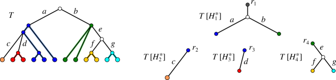
Figure 5: The tree $T$ is compatible with a partition $\mathcal{P}$ where leaves have the same color iff they are in the same set of $\mathcal{P}$. The edges in the unique separating set $H^{*}$ are labeled by lower-case letters and inner vertices $v$ for which $\varpi(v)=\emptyset$ are white. The colored vertices partition $H^{*}$ into $H_{\_}1^{*},H_{\_}2^{*},H_{\_}3^{*},$ and $H_{\_}4^{*}$. The subtrees $T[H_{\_}i^{*}]$ induced by the sets $H_{\_}i^{*}$ are shown on the right side. Note that a “planted rooted” with a dummy color was added to $T[H_{\_}1^{*}]$.

The edge set $H^{*}$ is naturally partitioned into disjoint components $H_{\_}i^{*}$ that are separated by colored vertices. More formally, two distinct edges $uv,u^{\prime}v^{\prime}\in H^{*}$ are in the same set $H_{\_}i^{*}$ if and only if at least one of the paths $P_{\_}{u,u^{\prime}}$, $P_{\_}{u,v^{\prime}}$, $P_{\_}{v,u^{\prime}}$, and $P_{\_}{v,v^{\prime}}$ does not contain a colored vertex; see Fig. 5 for an example. Note that both $uv$ and $u^{\prime}v^{\prime}$ contain at least one uncolored vertex and no two edges $h,h^{\prime}\in H_{\_}i^{*}$ are incident with the same colored vertex $u\in V(T)$. No uncolored vertex $v\in V(T)$ can be incident to edges that are contained in distinct sets $H_{\_}i^{*}$ and $H_{\_}j^{*}$. Thus, each edge set $H_{\_}i^{*}$ therefore defines a subtree

$$T[H_{\_}i^{*}]\coloneqq T[\{v\in V(T)\mid v\text{ is incident with some }e\in H_{\_}i^{*}\}]$$

All leaves of $T[H_{\_}i^{*}]$ are colored and all inner vertices except possibly the root, i.e., the $\preceq$-maximal element of $T[H_{\_}i^{*}]$, are uncolored. The root of $T[H_{\_}i^{*}]$ is either a colored vertex $u$ incident with a single edge $uw\in H_{\_}i^{*}$, or the uncolored root of $T[H_{\_}i^{*}]$ coincides with the root $\rho$ of $T$. If the latter special case occurs, we add a “planted rooted” with an additional dummy color not corresponding to a set of $\mathcal{P}$. The latter construction allows us to handle the component $T[H_{\_}i^{*}]$ containing the root of $T$ in the same manner as all other components. We write $r_{\_}i$ for the root (or the additional planted root in the special case), $L[H_{\_}i^{*}]$ for the leaf set and $V^{0}[H_{\_}i^{*}]$ for the set of inner vertices of $T[H_{\_}i^{*}]$ not including $r_{\_}i$. Note that the elements of $L[H_{\_}i^{*}]$ are not necessarily leaves of $T$. By construction, $\varpi(u)=\emptyset$ if and only if $u\in V^{0}[H_{\_}i^{*}]$. Moreover, we have $\varpi(u)\neq\varpi(v)$ for any two distinct $u,v\in L[H_{\_}i^{*}]\cup\{r_{\_}i\}$. We say that $H_{\_}i$ is a separating set on $T[H_{\_}i^{*}]$ if every path connecting two distinct leaves or a leaf and the root $r_{\_}i$ of $T[H_{\_}i^{*}]$ contains an edge $h\in H_{\_}i$. By way of example, for every choice of $H_{\_}4\subseteq\{e,f,g\}$ with $|H_{\_}4|\geq 2$, the set $H_{\_}4$ is a separating set on $T[H_{\_}4^{*}]$ in Fig. 5, while $H_{\_}4$ cannot be a separating set on $T[H_{\_}4^{*}]$ as soon as $|H_{\_}4|<2$. As we shall see in the next result, separating sets $H$ of $T$ can be characterized in terms of separating sets $H_{\_}i$ on the underlying trees $T[H_{\_}i^{*}]$.

Lemma 5.

Let $T$ and $\mathcal{P}$ be compatible. $H$ is a separating set for $(T,\mathcal{P})$ if and only if $H=\bigcup_{\_}iH_{\_}i$ such that every $H_{\_}i\subseteq H_{\_}i^{*}$ is a separating set for $T[H_{\_}i^{*}]$.

Proof.

Let $H$ be a separating set for $(T,\mathcal{P})$ and consider $H_{\_}i\coloneqq H\cap H_{\_}i^{*}$. If $H_{\_}i$ is not a separating set for $T[H_{\_}i^{*}]$ then there are two colored vertices $a$ and $b$ with $\varpi(a)\neq\varpi(b)$ connected by a path without an edge $h\in H$; a contradiction to Lemma 4. Conversely, let $H_{\_}i$ be a separating set for each component $T[H^{*}_{\_}i]$. Suppose $x\in A$ and $y\in B$ for distinct $A,B\in\mathcal{P}$. Hence, the path $P_{\_}{x,y}$ contains an edge $h=uv\in H^{*}$ which is contained in some $H_{\_}i^{*}$. Assume w.l.o.g. that $u$ is closer to $x$ than $v$. Let $u^{\prime}$ and $v^{\prime}$ be the last colored vertex on the path from $x$ to $u$ and on the path from $y$ to $v$, respectively. By construction, $u^{\prime}$ and $v^{\prime}$ are vertices in $T[H_{\_}i^{*}]$. In particular, since they are colored, we have $u^{\prime},v^{\prime}\in L[H_{\_}i^{*}]\cup\{r_{\_}i\}$. Since moreover $H_{\_}i$ is a separating set for $T[H_{\_}i^{*}]$, the subpath $P_{\_}{u^{\prime},v^{\prime}}$ of $P_{\_}{x,y}$ contains an edge $h\in H_{\_}i\subseteq H$. For $x,y\in A$ for some $A\in\mathcal{P}$, the path $P_{\_}{x,y}$ does not contains an edge $h\in H^{*}$ and, since $H\subseteq H^{*}$, also not an edge $h\in H$. In summary, $H=\bigcup_{\_}iH_{\_}i$ is separating for $(T,\mathcal{P})$. ∎

Lemma 5 suggests to study the separating sets $H_{\_}i$ for $T[H^{*}_{\_}i]$ independently of each other. In particular, $H$ is a separating set for $(T,\mathcal{P})$ if and only if every $H_{\_}i=H\cap H_{\_}i^{*}$ is a separating set for $T[H^{*}_{\_}i]$. We immediately observe that $h$ is an essential separating edge whenever $\{h\}=H^{*}_{\_}i$ for some component of $H^{*}$. This, in fact, characterizes the existence of essential separating edges.

Lemma 6.

An edge $h\in H_{\_}i^{*}$ is an essential separating edge if and only if $H^{*}_{\_}i=\{h\}$.

Proof.

If $H^{*}_{\_}i=\{h\}$, then $h$ must be contained in every separating set $H_{\_}i$ for $T[H^{*}_{\_}i]$ since otherwise there is no edge in $H_{\_}i$ between the root and the single leaf of $T[H^{*}_{\_}i]$, i.e., the two vertices adjacent to $h$. By Lemma 5, therefore, $h$ must be contained in every $H$ satisfying $\mathfrak{P}(T,H)=\mathcal{P}$. Hence, $h$ is an essential separating edge.

By contraposition, assume now that $H^{*}_{\_}i\neq\{h\}$ and thus, $|H_{\_}i^{*}|>1$. First we note that in this case $H_{\_}i^{*}$ contains at least three edges, two leaves, and one uncolored (interior) vertex. Denote by $H_{\_}L\subseteq H_{\_}i^{*}$ the set of edges $e_{\_}v=\{\operatorname{par}(v),v\}$ connecting the leaves $v\in L[H_{\_}i^{*}]$ of $T[H_{\_}i^{*}]$ to their parents. Clearly $H_{\_}L$ separates all leaves and the root of $T[H_{\_}i^{*}]$ from each other. Thus none of the edges that are not incident to a leaf is an essential separating edge, and in particular, the single edge $e=r_{\_}iu_{\_}i$, where $u_{\_}i$ is the unique child of $r_{\_}i$ in $T[H_{\_}i]$, is not an essential separating edge. On the other hand, for some $v\in L[H_{\_}i^{*}]$ consider the set $H_{\_}v$ comprising all edges of $H_{\_}i^{*}$ except the edges along the path from $v$ to unique child $u_{\_}i$ of the root. Clearly, $H_{\_}v$ also separates all leaves and the root of $T[H_{\_}i^{*}]$ from each other. Therefore $e_{\_}v$ is not an essential separating edge for all $v\in L[H_{\_}i^{*}]$. Consequently, $H_{\_}i^{*}$ does not contain any essential separating edge. ∎

We summarize the results of this section in

Theorem 1.

Let $T$ and $\mathcal{P}$ be compatible. An edge $vw\in E(T)$ is

(1)

an essential separating edge if and only if $\emptyset\neq\varpi(v)\neq\varpi(w)\neq\emptyset$,

(2)

a forbidden separating edge if and only if $\emptyset\neq\varpi(v)=\varpi(w)$.

and an ambiguous separating edge otherwise. In particular, the edges in $T$ can be classified as essential, forbidden, or ambiguous separating edges in $O(|L|)$.

Proof.

As an immediate consequence of Lemma 6, an edge $vw\in E(T)$ is an essential separating edge if and only if $\emptyset\neq\varpi(v)\neq\varpi(w)\neq\emptyset$. By Cor. 1, $vw\in E(T)$ is a forbidden separating edge if and only if $\emptyset\neq\varpi(v)=\varpi(w)$. By definition, $vw\in E(T)$ an ambiguous separating edge otherwise. By Lemma 2, $\varpi$ can be computed in $O(|L|)$ time. Since, for each edge, comparing the colors of its endpoints then takes constant time, the total effort to classify all $O(|L|)$ edges is bounded by $O(|L|)$. ∎

5 Edges of the Fitch Quotient Graph

In this section, we answer the question whether or not a pair $(x,y)$ with $x,y\in L$ is unambiguously present (or absent) in the Fitch graph given the knowledge of $T$ and $\mathcal{P}$. We first show that the edge set of Fitch quotient graph $\mathscr{F}(T,H)=\digamma(T,H)/\mathcal{P}$ completely determines the edges of the Fitch graph $\digamma(T,H)$.

Lemma 7.

Let $T$ and $\mathcal{P}$ be $H$-compatible and $A,B\in\mathcal{P}$. Then there are $x\in A,y\in B$ with $(x,y)\in E(\digamma(T,H))$ if and only if $(x^{\prime},y^{\prime})\in E(\digamma(T,H))$ for all $x^{\prime}\in A,y^{\prime}\in B$.

Proof.

Suppose there are $x\in A$ and $y\in B$ such that $(x,y)\in\digamma(T,H)$, i.e., the path $P\coloneqq P_{\_}{\operatorname{lca}_{\_}T(x,y)y}\subseteq E(T)$ connecting $\operatorname{lca}_{\_}T(x,y)$ and $y$ contains an edge $e=uv\in H$. In particular, $A$ and $B$ must be distinct, $y\in L(T(v))$ and $x\notin L(T(v))$. The latter implies $x^{\prime}\notin L(T(v))$ for any $x^{\prime}\in A$ since otherwise $P_{\_}{x,x^{\prime}}$ contains $e$ contradicting $x,x^{\prime}\in A$. By similar arguments, $y^{\prime}\in L(T(v))$ holds for any $y^{\prime}\in B$. Hence, for any $x^{\prime}\in A$ and $y^{\prime}\in B$, we obtain $u\preceq_{\_}T\operatorname{lca}_{\_}T(x^{\prime},y^{\prime})\eqqcolon w$. In particular, since $y^{\prime}\preceq_{\_}Tv\prec_{\_}Tu\preceq_{\_}Tw$, the path $P_{\_}{w,y^{\prime}}$ contains $e$, and thus $(x^{\prime},y^{\prime})\in E(\digamma(T,H))$. The converse follows trivially from the fact that $A$ and $B$ are sets in the partition $\mathcal{P}$ and thus non-empty. ∎

It therefore suffices to consider $\mathscr{F}(T,H)$:

Corollary 2.

Let $T$ and $\mathcal{P}$ be $H$-compatible, $A,B\in\mathcal{P}$ and $x\in A,y\in B$. Then, $(x,y)\in E(\digamma(T,H))$ if and only if $(A,B)\in E(\mathscr{F}(T,H))$.

We first derive sufficient conditions for essential pairs $(A,B)\in E(\mathscr{F}(T,H))$ and forbidden pairs $(A,B)\notin E(\mathscr{F}(T,H))$.

Proposition 4.

Let $T$ and $\mathcal{P}$ be compatible. Then the following statements hold for all distinct $A,B\in\mathcal{P}$:

(i)

If there is a colored vertex $v\in V^{0}(T)$ such that $\operatorname{lca}(B)\prec v\preceq\operatorname{lca}(A\cup B)$, then $(A,B)$ is essential.

(ii)

If $\operatorname{lca}(A)\prec\operatorname{lca}(B)$, then $(A,B)$ is forbidden.

Proof.

(i) Since $v\in V^{0}(T)$ is colored, it holds that $\varpi(v)\neq\emptyset$. By construction, there is a leaf $x\in A$ and $y\in B$ such that $y\preceq\operatorname{lca}(B)\prec v\preceq\operatorname{lca}(x,y)\eqqcolon u$. By assumption, we have $\operatorname{lca}(B)\prec v$ and thus $\varpi(v)\neq B$. By Lemma 4 and since moreover $\varpi(y)=B\neq\varpi(v)$, the path $P_{\_}{v,y}$, which is a subpath of $P_{\_}{u,y}$, contains at least one edge $e\in H$ for any choice of $H$. Hence, we have $(x,y)\in E(\digamma(T,H))$ and by Cor. 2 $(A,B)$ is essential.

(ii) Since $\operatorname{lca}(A)\prec\operatorname{lca}(B)$, we have $\varpi(\operatorname{lca}(A))=A\neq B=\varpi(\operatorname{lca}(B))$. Moreover, there are leaves $x\in A$ and $y\in B$ such that $x\preceq\operatorname{lca}(A)\prec\operatorname{lca}(x,y)=\operatorname{lca}(B)$. Cor. 2 together with $\varpi(\operatorname{lca}(B))=\varpi(y)=B$ implies that the path $P_{\_}{\operatorname{lca}(B),y}=P_{\_}{\operatorname{lca}(x,y),y}$ contains no edge $w\in H$. Thus $(x,y)\notin E(\digamma(T,H))$ for any choice of $H$, which, by Cor. 2, implies that $(A,B)$ is forbidden. ∎

Note that the vertex $\operatorname{lca}(B)$ in Prop. 4 must be colored. In particular, if Prop. 4(ii) is satisfied, then $\operatorname{lca}(A)\prec\operatorname{lca}(B)=\operatorname{lca}(A\cup B)$ and thus, Prop. 4(i) is satisfied by interchanging the role of $A$ and $B$. In summary, we obtain

Corollary 3.

Let $T$ and $\mathcal{P}$ be compatible. If $\operatorname{lca}(A)\prec\operatorname{lca}(B)$ for two $A,B\in\mathcal{P}$, then $(B,A)$ is essential and $(A,B)$ is forbidden.

Recall that $\operatorname{lca}(A)=\operatorname{lca}(B)$ cannot occur for distinct $A,B\in\mathcal{P}$ (Hellmuth et al., 2021b, Thm. 4.5). By Cor. 3, we can unambiguously infer the edges between $A$ and $B$ in $\mathscr{F}$ whenever $\operatorname{lca}(A)$ and $\operatorname{lca}(B)$ are comparable. Whenever $\operatorname{lca}(A)$ and $\operatorname{lca}(B)$ are incomparable and there is no colored vertex $v\in V^{0}(T)$ such that $\operatorname{lca}(B)\prec v\preceq\operatorname{lca}(A\cup B)$, however, we cannot make a statement about the presence of $(A,B)$ in $E(\mathscr{F})$.

The construction of the separating sets $H_{\_}v$ and $H_{\_}L$ in the proof of Lemma 6 can be used to infer the following statement of edges in Fitch graphs.

Lemma 8.

Let $T$ and $\mathcal{P}$ be compatible and $A,B\in\mathcal{P}$ be distinct. If $\operatorname{lca}(A)$ and $\operatorname{lca}(B)$ are $\preceq$-incomparable and there is no colored vertex $v$ with $\operatorname{lca}(B)\prec v\preceq\operatorname{lca}(A\cup B)$, then $(A,B)$ is ambiguous.

Proof.

All last common ancestors ($\operatorname{lca}$) are taken w.r.t. $T$. By assumption, $w\coloneqq\operatorname{lca}(A\cup B)$ is an uncolored inner vertex and thus also an uncolored inner vertex of $T[H_{\_}i^{*}]$ for some component $H^{*}_{\_}i$ of $H^{*}$ and thus $\operatorname{lca}(x,y)=w$ for all $x\in A$ and $y\in B$. Moreover, since there is no colored vertex on the path $P_{\_}{w,\operatorname{lca}(B)}$ with exception of $b\coloneqq\operatorname{lca}(B)$, we have $b\in L[H^{*}_{\_}i]$. Let $e_{\_}b=\operatorname{par}(b)b$ and denote by $H_{\_}b$ the set of all edges of $H^{*}$ except the edges along the path $P_{\_}{u_{\_}i,b}$ from the unique child $u_{\_}i$ of the root $r_{\_}i$ to $b$. By Lemma 5 and the arguments in the proof of Lemma 6, $H_{\_}b$ is a separating set for $(T,\mathcal{P})$. Since $r_{\_}i$ only has a single child and $w\coloneqq\operatorname{lca}(A\cup B)$ has at least two, we observe that $w\preceq u_{\_}i$, and thus, $w$ lies along both the path from $u_{\_}i$ to $b$. Therefore, $P_{\_}{w,b}$ is a subpath of $P_{\_}{u_{\_}i,w}$ and thus also does not contain an edge of $H_{\_}b$. Moreover, for any $y\in B$, Lemma 4 and $\varpi(b)=B=\varpi(y)$ imply that the path $P_{\_}{b,y}$ also does not contain an edge in $H_{\_}b$. Since in addition, for any $a\in A$ and $b\in B$, the path $P_{\_}{\operatorname{lca}(x,y)=w,y}$ is composed of the paths $P_{\_}{w,b}$ and $P_{\_}{b,y}$, we obtain $(A,B)\notin\mathscr{F}(T,H_{\_}b)$ by Cor. 2. On the other hand, $e_{\_}b\in H^{*}$ is an edge on the path $P_{\_}{\operatorname{lca}(x,y)=w,y}$ for all $a\in A$ and $b\in B$, which, by Cor. 2, implies $(A,B)\in\mathscr{F}(T,H^{*})$. In summary, therefore, $(A,B)$ is ambiguous. ∎

Lemma 8 together with the observation that $(A,B)\notin\mathscr{F}(T,H)$ implies $(B,A)\in\mathscr{F}(T,H)$ for any two distinct $A,B\in\mathcal{P}$ yields

Corollary 4.

Let $T$ and $\mathcal{P}$ be compatible and $A,B\in\mathcal{P}$ be distinct. If there is a component $H_{\_}i^{*}$ of $H^{*}$ with $\operatorname{lca}_{\_}T(A)$ and $\operatorname{lca}_{\_}T(B)$ being distinct leaves of $T[H_{\_}i^{*}]$, then there exist choices $H_{\_}1$, $H_{\_}2$, and $H_{\_}3$ of separating edge sets such that

• $(A,B)\in\mathscr{F}(T,H_{\_}1)$ and $(B,A)\in\mathscr{F}(T,H_{\_}1)$,

• $(A,B)\in\mathscr{F}(T,H_{\_}2)$ and $(B,A)\notin\mathscr{F}(T,H_{\_}2)$, and

• $(A,B)\notin\mathscr{F}(T,H_{\_}3)$ and $(B,A)\in\mathscr{F}(T,H_{\_}3)$.

The partial results above show that the choices of directions of arc(s) between $A,B\in\mathcal{P}$ in the quotient graph $\mathscr{F}$ depend in the $\preceq_{\_}T$-order of $\operatorname{lca}(A)$ and $\operatorname{lca}(B)$ and the positioning of colored vertices along the unique path connecting $\operatorname{lca}(A)$ and $\operatorname{lca}(B)$ in $T$.

Lemma 9.

Let $T$ and $\mathcal{P}$ be compatible and $A,B\in\mathcal{P}$ be distinct, and suppose there is no colored vertex $v\in V^{0}(T)$ such that $\operatorname{lca}(B)\prec v\preceq\operatorname{lca}(A\cup B)$. Then $(A,B)$ is forbidden if and only if $\operatorname{lca}(A)\prec\operatorname{lca}(B)$, and otherwise $(A,B)$ is ambiguous.

Proof.

Assume that there is no colored vertex $v\in V^{0}(T)$ such that $\operatorname{lca}(B)\prec v\preceq\operatorname{lca}(A\cup B)$. If $\operatorname{lca}(A)\prec\operatorname{lca}(B)$, Prop. 4(ii) implies that $(A,B)\notin E(\mathscr{F}(T,H))$ for all choices of $H$. For the converse, suppose that $\operatorname{lca}(A)\not\prec\operatorname{lca}(B)$. The case $\operatorname{lca}(A)=\operatorname{lca}(B)$ is not possible since $A\neq B$ and $T$ and $\mathcal{P}$ are compatible. Moreover, $\operatorname{lca}(B)\prec\operatorname{lca}(A)$ is not possible since otherwise the colored vertex $\operatorname{lca}(A)$ satisfies $\operatorname{lca}(B)\prec\operatorname{lca}(A)=\operatorname{lca}(A\cup B)$; contradicting the assumption. Therefore, it remains to consider the case that $\operatorname{lca}(A)$ and $\operatorname{lca}(B)$ are $\preceq$-incomparable. By assumption, all vertices on the path $P$ except $\operatorname{lca}(B)$ are uncolored. Therefore, we can apply Lemma 8 to conclude that $(A,B)$ is ambiguous. ∎

Combining Prop. 4 and Lemma 9 yields the following characterization of edges that are unambiguously present or absent, and edges whose presence or absence depends on the choice of $H$.

Theorem 2.

Let $T$ and $\mathcal{P}$ be compatible and $A,B\in\mathcal{P}$ be distinct. Then the following statements hold:

(1)

$(A,B)$ is essential if and only if there is a colored vertex $v\in V^{0}(T)$ such that $\operatorname{lca}(B)\prec v\preceq\operatorname{lca}(A\cup B)$.

(2)

$(A,B)$ is forbidden if and only if $\operatorname{lca}(A)\prec\operatorname{lca}(B)$.

(3)

$(A,B)$ is ambiguous if and only if $\operatorname{lca}(A)$ and $\operatorname{lca}(B)$ are $\preceq$-incomparable and there is no colored vertex $v\in V^{0}(T)$ such that $\operatorname{lca}(B)\prec v\preceq\operatorname{lca}(A\cup B)$.

Proof.

(1) If there is a colored vertex $v\in V^{0}(T)$ such that $\operatorname{lca}(B)\prec v\preceq\operatorname{lca}(A\cup B)$, then $(A,B)$ is essential by Prop. 4(i). If there is no colored vertex $v\in V^{0}(T)$ such that $\operatorname{lca}(B)\prec v\preceq\operatorname{lca}(A\cup B)$, then, by Lemma 9, $(A,B)$ is forbidden or ambiguous and thus not essential.

(2) If $\operatorname{lca}(A)\prec\operatorname{lca}(B)$, then $\operatorname{lca}(B)=\operatorname{lca}(A\cup B)$. Hence, there is no colored vertex $v\in V^{0}(T)$ such that $\operatorname{lca}(B)\prec v\preceq\operatorname{lca}(A\cup B)$. By Lemma 9, this yields that $(A,B)$ is forbidden. For the converse, recall that by (Hellmuth et al., 2021b, Thm. 4.5), $\operatorname{lca}(A)=\operatorname{lca}(B)$ is not possible. If $\operatorname{lca}(B)\prec\operatorname{lca}(A)$, then $(A,B)$ is essential by Cor. 3. If $\operatorname{lca}(A)$ and $\operatorname{lca}(B)$ are $\preceq$-incomparable, then Prop. 4(i) and Lemma 9 imply that $(A,B)$ must be essential or ambiguous, respectively. In summary, $\operatorname{lca}(A)\not\prec\operatorname{lca}(B)$ implies that $(A,B)$ is not forbidden.

(3) If $\operatorname{lca}(A)$ and $\operatorname{lca}(B)$ are $\preceq$-incomparable and there is no colored vertex $v\in V^{0}(T)$ such that $\operatorname{lca}(B)\prec v\preceq\operatorname{lca}(A\cup B)$, then $(A,B)$ is ambiguous by Lemma 9. If $\operatorname{lca}(A)$ and $\operatorname{lca}(B)$ are comparable, then Cor. 3 implies that $(A,B)$ is essential or forbidden. If there is a colored vertex $v\in V^{0}(T)$ such that $\operatorname{lca}(B)\prec v\preceq\operatorname{lca}(A\cup B)$, then $(A,B)$ is essential by statement (1). By contraposition, therefore, the only-if-part of statement (3) is also true. ∎

Corollary 5.

Let $T$ and $\mathcal{P}$ be compatible. After an $O(|L|)$ preprocessing step, we can query, for two distinct $A,B\in\mathcal{P}$, in constant time whether $(A,B)$ is essential, forbidden, or ambiguous for $(T,\mathcal{P})$. In particular, we can make these assignments for all distinct $A,B\in\mathcal{P}$ in $O(|L|+|\mathcal{P}|^{2})$ total time.

Proof.

We compute $\varpi$ and $\operatorname{lca}(A)$ for all $\mathcal{P}$ in $O(|L|)$ according to Lemma 2. In particular, this procedure already includes the construction an LCA data structure that enables constant-time queries for the last common ancestor for any pair $v,v^{\prime}\in V(T)$. We continue by computing, for each $v\in V(T)$, the unique $\preceq$-minimal colored vertex $u$ that is a strict ancestor of $v$, i.e., that satisfies $v\prec u$, if such a vertex exists. We achieve this by filling a map lcsa (for “lowest colored strict ancestor”) in a top-down traversal of $T$. More precisely, we initialize $\texttt{lcsa}(\rho)=\emptyset$ for the root $\rho$. Then, for each vertex $v\in V(T)\setminus\{\rho\}$, we set $\texttt{lcsa}(v)=\operatorname{par}_{\_}T(v)$ if $\operatorname{par}_{\_}T(v)$ is a colored vertex; and $\texttt{lcsa}(v)=\texttt{lcsa}(\operatorname{par}_{\_}T(v))$ otherwise. We are now able to query in constant time, whether, for two vertices $u,v\in V(T)$ with $v\prec u$, there is a colored vertex $w$ such that $v\prec w\preceq u$ by just evaluating whether $\operatorname{lca}(\texttt{lcsa}(v),u)=u$. Checking whether or not $\operatorname{lca}(A\cup B)=\operatorname{lca}(\operatorname{lca}(A),\operatorname{lca}(B))$ equals $\operatorname{lca}(B)$ also determines whether or not $\operatorname{lca}(A)\prec\operatorname{lca}(B)$ since we know that $\operatorname{lca}(A)\neq\operatorname{lca}(B)$ for distinct $A,B\in\mathcal{P}$. Similarly, $\operatorname{lca}(A\cup B)\notin\{\operatorname{lca}(A),\operatorname{lca}(B)\}$ implies that $\operatorname{lca}(A)$ and $\operatorname{lca}(B)$ are $\preceq$-incomparable. In summary, the conditions of Thm. 2 can therefore be evaluated in constant time for each of the $O(|\mathcal{P}|^{2})$ pairs $(A,B)$. ∎

It is important to note that the choice of presence/absence for ambiguous edges is not arbitrary. First, in the quotient graph $\mathscr{F}(T,H)$ at least one of $(A,B)$ and $(B,A)$ is always present. Second, $\mathscr{F}(T,H)$ is itself a Fitch graph, and thus characterized by forbidden induced subgraphs on three vertices (Geiß et al., 2018; Hellmuth and Seemann, 2019). The condition that an edge must be present in at least one direction reduced the possibilities to only four allowed configurations on three vertices, namely the triangles A1, A4, A5, and A6 in Fig. 2 of (Geiß et al., 2018).

6 Edges of Fitch Quotient Graphs for Refinements of Trees

Let us now turn to the case that $T$ and $\mathcal{P}$ are refinement-compatible but not necessarily compatible. We first collect some basic results concerning ancestry in trees that is preserved upon refinement.

Lemma 10.

Let $T^{\prime}$ be a refinement of a tree $T$ with leaf set $L$ and $uv\in E(T)$. Then the following statements hold for non-empty $X\subseteq L$.

(i)

If $\operatorname{lca}_{\_}{T}(X)\preceq_{\_}Tv$, then $\operatorname{lca}_{\_}{T^{\prime}}(X)\preceq_{\_}{T^{\prime}}v^{\prime}$ for the vertex $v^{\prime}\in V(T^{\prime})$ satisfying $L(T(v))=L(T^{\prime}(v^{\prime}))$.

(ii)

If $u\preceq_{\_}{T}\operatorname{lca}_{\_}{T}(X)$ and $L(T(v))\cap X\neq\emptyset$, then $v^{\prime}\prec_{\_}{T^{\prime}}\operatorname{lca}_{\_}{T^{\prime}}(X)$ for the vertex $v^{\prime}\in V(T^{\prime})$ satisfying $L(T(v))=L(T^{\prime}(v^{\prime}))$.

(iii)

If $\operatorname{lca}_{\_}{T}(X)$ and $\operatorname{lca}_{\_}{T}(\tilde{X})$ are $\preceq_{\_}{T}$-incomparable for some $\tilde{X}\subseteq L$, then $\operatorname{lca}_{\_}{T^{\prime}}(X)$ and $\operatorname{lca}_{\_}{T^{\prime}}(\tilde{X})$ are $\preceq_{\_}{T^{\prime}}$-incomparable.

Proof.

Note first that, since $T^{\prime}$ is a refinement of $T$, we have $\mathcal{H}(T)\subseteq\mathcal{H}(T^{\prime})$, and thus the vertex $v^{\prime}\in V(T^{\prime})$ satisfying $L(T(v))=L(T^{\prime}(v^{\prime}))$ exists for every $v\in V(T)$. First suppose $\operatorname{lca}_{\_}{T}(X)\preceq_{\_}Tv$. Therefore, we have $X\subseteq L(T(v))=L(T^{\prime}(v^{\prime}))$. Together with the fact that $X$ is non-empty, this implies that $\operatorname{lca}_{\_}{T^{\prime}}(X)\preceq_{\_}{T^{\prime}}v^{\prime}$, and thus statement (i). Suppose $u\preceq_{\_}{T}\operatorname{lca}_{\_}{T}(X)$ and $L(T(v))\cap X\neq\emptyset$. Recall that, by convention, $uv\in E(T)$ implies that $v\prec_{\_}Tu$. Hence, $v\prec_{\_}Tu\preceq_{\_}{T}\operatorname{lca}_{\_}{T}(X)$ and, therefore, $X\not\subseteq L(T(v))=L(T^{\prime}(v^{\prime}))$. Since by assumption there is an $x\in X$ such that $x\in L(T(v))=L(T^{\prime}(v^{\prime}))$, $v^{\prime}$ and $\operatorname{lca}_{\_}{T^{\prime}}(X)$ are both ancestors of $x$ and thus $\preceq_{\_}{T^{\prime}}$-comparable. Together with $X\not\subseteq L(T^{\prime}(v^{\prime}))$, this yields $v^{\prime}\prec_{\_}{T^{\prime}}\operatorname{lca}_{\_}{T^{\prime}}(X)$ and thus statement (ii) is true. Finally, suppose $\operatorname{lca}_{\_}{T}(X)$ and $\operatorname{lca}_{\_}{T}(\tilde{X})$ are $\preceq_{\_}{T}$-incomparable for some $\tilde{X}\subseteq L$, set $u=\operatorname{lca}_{\_}{T}(X)$ and $\tilde{u}=\operatorname{lca}_{\_}{T}(\tilde{X})$, and let $u^{\prime},\tilde{u}^{\prime}\in V(T^{\prime})$ be the vertices satisfying $L(T(u))=L(T^{\prime}(u^{\prime}))$ and $L(T(\tilde{u}))=L(T^{\prime}(\tilde{u}^{\prime}))$. Since $u$ and $\tilde{u}$ are $\preceq_{\_}{T}$-incomparable, we have $\emptyset=L(T(u))\cap L(T(\tilde{u}))=L(T(u^{\prime}))\cap L(T(\tilde{u}^{\prime}))$, and thus $u^{\prime}$ and $\tilde{u}^{\prime}$ are $\preceq_{\_}{T^{\prime}}$-incomparable. Moreover, $X\subseteq L(T(u))=L(T^{\prime}(u^{\prime}))$ and $\tilde{X}\subseteq L(T(\tilde{u}))=L(T^{\prime}(\tilde{u}^{\prime}))$ implies $\operatorname{lca}_{\_}{T^{\prime}}(X)\prec_{\_}{T^{\prime}}u^{\prime}$ and $\operatorname{lca}_{\_}{T^{\prime}}(\tilde{X})\prec_{\_}{T^{\prime}}\tilde{u}^{\prime}$. This together with $u^{\prime}$ and $\tilde{u}^{\prime}$ being $\preceq_{\_}{T^{\prime}}$-incomparable implies statement (iii). ∎

We next derive sufficient conditions for pairs $(A,B)$ that are r-essential or r-forbidden, respectively.

Proposition 5.

Let $T$ and $\mathcal{P}$ be r-compatible. Then for all $A,B\in\mathcal{P}$ it holds

(i)

If the path $P_{\_}{\operatorname{lca}_{\_}{T}(A\cup B),\operatorname{lca}_{\_}{T}(B)}$ contains a colored edge, then $(A,B)$ is r-essential.

(ii)

If $\operatorname{lca}_{\_}{T}(A)\prec_{\_}T\operatorname{lca}_{\_}{T}(B)$ and $\gamma(\operatorname{lca}_{\_}{T}(B)v)=B$ for the vertex $v\in\operatorname{child}_{\_}{T}(\operatorname{lca}_{\_}{T}(B))$ satisfying $\operatorname{lca}_{\_}{T}(A)\preceq_{\_}Tv$, then $(A,B)$ is r-forbidden.

(iii)

If the path $P_{\_}{u,\operatorname{lca}_{\_}{T}(A)}$ with $u\coloneqq\operatorname{lca}_{\_}{T}(A\cup B)\neq\rho_{\_}T$ contains a colored edge $e$ with $\gamma(e)=\gamma(\operatorname{par}_{\_}T(u)u)=C\in\mathcal{P}$, then $(A,B)$ is r-essential.

Proof.

All three statements are proven by considering an arbitrary refinement $T^{\prime}$ of $T$ and a set $H\subseteq E(T^{\prime})$ satisfying $\mathfrak{P}(T^{\prime},H)=\mathcal{P}$. In particular, the vertex coloring $\varpi\colon V(T^{\prime})\to\mathcal{P}\cup\{\emptyset\}$ is well-defined for any such $T^{\prime}$ and $\mathcal{P}$.

(i) Suppose that there is an edge $uv\in E(P_{\_}{\operatorname{lca}_{\_}{T}(A\cup B),\operatorname{lca}_{\_}{T}(B)})$ with $\gamma(uv)=C$ for some $C\in\mathcal{P}$. In particular, this implies $\operatorname{lca}_{\_}{T}(B)\prec_{\_}T\operatorname{lca}_{\_}{T}(A\cup B)$. We have to show that $(A,B)\in\mathscr{F}(T^{\prime},H)$. Lemma 10(i) together with $\operatorname{lca}_{\_}{T}(B)\preceq_{\_}Tv$ implies $\operatorname{lca}_{\_}{T^{\prime}}(B)\preceq_{\_}{T^{\prime}}v^{\prime}$ where $v^{\prime}$ is the vertex in $T^{\prime}$ satisfying $L(T^{\prime}(v^{\prime}))=L(T(v))$. By assumption, $u\preceq_{\_}{T}\operatorname{lca}_{\_}{T}(A\cup B)$ and $\emptyset\neq B\subseteq L(T(v))\cap(A\cup B)$. Together with Lemma 10(ii), this implies $v^{\prime}\prec_{\_}{T^{\prime}}\operatorname{lca}_{\_}{T^{\prime}}(A\cup B)$. Since $\gamma(uv)=C$, we have $L(T^{\prime}(v^{\prime}))\cap C=L(T(v))\cap C\neq\emptyset$ and also $L(T^{\prime}(v^{\prime}))\setminus C=L(T(v))\setminus C\neq\emptyset$. Therefore, $v^{\prime}$ lies on the path that connects two distinct vertices from $C$, and thus $\varpi(v^{\prime})=C$. Moreover, since $B\subseteq L(T(v))=L(T^{\prime}(v^{\prime}))$ and $L(T^{\prime}(v^{\prime}))\setminus C\neq\emptyset$, we have $B\neq C$. Together with $\varpi(\operatorname{lca}_{\_}{T^{\prime}}(B))=B$ and $\varpi(v^{\prime})=C$, this implies $\operatorname{lca}_{\_}{T^{\prime}}(B)\neq v^{\prime}$, and thus $\operatorname{lca}_{\_}{T^{\prime}}(B)\prec_{\_}{T^{\prime}}v^{\prime}$. In summary, there is a colored vertex $v^{\prime}\in V^{0}(T^{\prime})$ such that $\operatorname{lca}_{\_}{T^{\prime}}(B)\prec_{\_}{T^{\prime}}v^{\prime}\preceq_{\_}{T^{\prime}}\operatorname{lca}_{\_}{T^{\prime}}(A\cup B)=\operatorname{lca}_{\_}{T^{\prime}}(\operatorname{lca}_{\_}{T^{\prime}}(A),\operatorname{lca}_{\_}{T^{\prime}}(B))$. Hence, we can apply Thm. 2(1) to conclude that the statement is true.

(ii) Suppose $\operatorname{lca}_{\_}{T}(A)\prec_{\_}T\operatorname{lca}_{\_}{T}(B)$ and $\gamma(\operatorname{lca}_{\_}{T}(B)v)=B$ for the vertex $v\in\operatorname{child}_{\_}{T}(\operatorname{lca}_{\_}{T}(B))$ satisfying $\operatorname{lca}_{\_}{T}(A)\preceq_{\_}Tv$. We have to show that $(A,B)\notin\mathscr{F}(T^{\prime},H)$. Lemma 10(i) together with $\operatorname{lca}_{\_}{T}(A)\preceq_{\_}Tv$ implies $\operatorname{lca}_{\_}{T^{\prime}}(A)\preceq_{\_}{T^{\prime}}v^{\prime}$ where $v^{\prime}$ is the vertex in $T^{\prime}$ satisfying $L(T^{\prime}(v^{\prime}))=L(T(v))$. Since $\gamma(\operatorname{lca}_{\_}{T}(B)v)=B$, we have $L(T(v))\cap B\neq\emptyset$ which together with Lemma 10(ii) implies $v^{\prime}\prec_{\_}{T^{\prime}}\operatorname{lca}_{\_}{T^{\prime}}(B)$. In summary, we have $\operatorname{lca}_{\_}{T^{\prime}}(A)\preceq_{\_}{T^{\prime}}v^{\prime}\prec_{\_}{T^{\prime}}\operatorname{lca}_{\_}{T^{\prime}}(B)$. Now apply Prop. 4(ii).

(iii) By assumption, there is an edge $vw\in E(P_{\_}{u,\operatorname{lca}_{\_}{T}(A)})$, where $u\coloneqq\operatorname{lca}_{\_}{T}(A\cup B)$, of color $\gamma(vw)=C=\gamma(\operatorname{par}_{\_}T(u)u)$. We observe that $A\neq C$, and $L(T(w))\cap C\neq\emptyset$. Lemma 10(ii), $v\preceq_{\_}{T}u=\operatorname{lca}_{\_}{T}(A\cup B)$, and $L(T(w))\cap C\neq\emptyset$ imply $w^{\prime}\prec_{\_}{T^{\prime}}\operatorname{lca}_{\_}{T^{\prime}}(A\cup B)\eqqcolon u^{\prime}$ for the vertex $w^{\prime}\in V(T^{\prime})$ satisfying $L(T^{\prime}(w^{\prime}))=L(T(w))$. From $\gamma(\operatorname{par}_{\_}T(u)u)=C$, we conclude $C\setminus L(T(u))\neq\emptyset$ and since $\operatorname{lca}_{\_}{T}(B)\preceq_{\_}{T}u$ also $C\neq B$. Since moreover $L(T^{\prime}(u^{\prime}))\subseteq L(T(u))$, we also have $C\setminus L(T^{\prime}(u^{\prime}))\neq\emptyset$. Therefore and since there is a vertex $c\in C$ with $c\preceq_{\_}{T^{\prime}}w^{\prime}\prec_{\_}{T^{\prime}}u^{\prime}$, we must have $c\preceq_{\_}{T^{\prime}}w^{\prime}\prec_{\_}{T^{\prime}}u^{\prime}\prec_{\_}{T^{\prime}}\operatorname{lca}_{\_}{T}(C)$. In particular, therefore, vertex $u^{\prime}$ lies on the path connecting two vertices of $C$, and thus it is a vertex of color $\varpi(u^{\prime})=C$ on the path $P_{\_}{u^{\prime},\operatorname{lca}_{\_}{T^{\prime}}(B)}$. We have $\varpi(u^{\prime})=C\neq B=\varpi(\operatorname{lca}_{\_}{T^{\prime}}(B))$ and thus $\operatorname{lca}_{\_}{T^{\prime}}(B)\prec_{\_}{T^{\prime}}u^{\prime}$. Now apply Thm. 2(1). ∎

We note that the conditions in Prop. 5(ii) are a special case of those in Prop. 5(i), since the edge $\operatorname{lca}_{\_}{T}(A)v$ is a colored edge on the path $P_{\_}{\operatorname{lca}_{\_}{T}(A\cup B),\operatorname{lca}_{\_}{T}(B)}$, and thus we obtain

Corollary 6.

Let $T$ and $\mathcal{P}$ be r-compatible. If, for $A,B\in\mathcal{P}$, it holds $\operatorname{lca}_{\_}{T}(A)\prec_{\_}T\operatorname{lca}_{\_}{T}(B)$ and $\gamma(\operatorname{lca}_{\_}{T}(B)v)=B$ for the vertex $v\in\operatorname{child}_{\_}{T}(\operatorname{lca}(B))$ satisfying $\operatorname{lca}_{\_}{T}(A)\preceq_{\_}Tv$, then $(B,A)$ is r-essential and $(A,B)$ is r-forbidden.

Similar to the previous section, we will show that it is not possible to unambiguously assign a direction for all pairs $(A,B)$ that are not covered by Prop. 5. Even though we do not want to construct the set of all compatible refinement explicitly, it will be helpful to study the properties of two special representatives. A compatible refinement $T^{\prime}$ for an r-compatible pair $(T,\mathcal{P})$ can be constructed in linear time (Hellmuth et al., 2021b, Thm. 7.5). To this end, Hellmuth et al. (2021b) considered the set

$$\mathfrak{Y}(T,\mathcal{P})\coloneqq\left\{A\in\mathcal{P}\mid\exists B\in\mathcal{P}\colon B\neq A,\,B\cap\operatorname{cl}(A)\neq\emptyset\text{ and }\operatorname{cl}_{\_}{T}(A)\subseteq\operatorname{cl}_{\_}{T}(B)\right\}\,,$$ (1)

which contains the sets $A\in\mathcal{P}$ for which the vertex $u\coloneqq\operatorname{lca}_{\_}{T}(A)\in V(T)$ is “not resolved enough”. The conditions $B\cap\operatorname{cl}_{\_}{T}(A)\neq\emptyset$ and $\operatorname{cl}_{\_}{T}(A)\subseteq\operatorname{cl}_{\_}{T}(B)$ are equivalent to $u$ having a child $v$ such that $\gamma(uv)=B$.

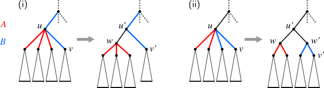
Figure 6: Necessary refinement steps for a set $A\in\mathfrak{Y}(T,\mathcal{P})$. In both examples, there is a vertex $v\in\operatorname{child}_{\_}{T}(u\coloneqq\operatorname{lca}_{\_}{T}(A))$ such that $\gamma(uv)=B$ for some $B\in\mathcal{P}\setminus\{A\}$. The two cases (i) $u\prec_{\_}{T}\operatorname{lca}_{\_}{T}(B)$ and (ii) $u=\operatorname{lca}_{\_}{T}(B)$ are possible. The latter case implies that also $B\in\mathfrak{Y}(T,\mathcal{P})$.

To see this, suppose first $B\cap\operatorname{cl}_{\_}T(A)\neq\emptyset$ and $\operatorname{cl}_{\_}{T}(A)\subseteq\operatorname{cl}_{\_}{T}(B)$. Since $A\neq B$ and $B\cap L(T(u))=B\cap\operatorname{cl}_{\_}T(A)\neq\emptyset$, we can conclude that $L(T(u))$ contains at least one vertex of both $A$ and $B$. In particular, $u$ is an inner vertex and has a child $v$ such that $B\cap L(T(v))\neq\emptyset$. However, $\operatorname{cl}_{\_}{T}(A)\subseteq\operatorname{cl}_{\_}{T}(B)$ is equivalent to $u\preceq_{\_}T\operatorname{lca}_{\_}{T}(B)$ and thus $B\setminus L(T(v))\neq\emptyset$. Therefore, the edge $uv$ lies on the path connecting two vertices from $B$, and thus $\gamma(uv)=B$. Conversely, if $\gamma(\operatorname{lca}_{\_}{T}(A)v)=B$, then $B\cap L(T(v))\neq\emptyset$ and $B\setminus L(T(v))\neq\emptyset$ implying $B\cap\operatorname{cl}_{\_}T(A)\neq\emptyset$ and $\operatorname{cl}_{\_}{T}(A)\subseteq\operatorname{cl}_{\_}{T}(B)$, respectively, see Fig. 6 for a graphical depiction of the situation.

We thus obtain

$$\mathfrak{Y}(T,\mathcal{P})=\left\{A\in\mathcal{P}\mid\exists v\in\operatorname{child}_{\_}{T}(\operatorname{lca}_{\_}{T}(A))\colon\gamma(\operatorname{lca}_{\_}{T}(A)v)=B\in\mathcal{P}\setminus\{A\})\right\}.$$ (2)

By (Hellmuth et al., 2021b, Lemma 5.6), the tree $T^{*}$ satisfying

$$\mathcal{H}(T^{*})=\mathcal{H}(T)\cup\bigcup_{\_}{A\in\mathfrak{Y}(T,\mathcal{P})}\{\bigcup_{\_}{\quad\begin{subarray}{c}v\in\operatorname{child}_{\_}{T}(\operatorname{lca}_{\_}{T}(A)),\\ \gamma(\operatorname{lca}_{\_}{T}(A)v)=A\end{subarray}}L(T(v))\quad\}$$ (3)

is a refinement of $T$ that is compatible with $\mathcal{P}$. Algorithmically, $T^{*}$ is obtained by introducing, for each $A\in\mathfrak{Y}(T,\mathcal{P})$, a new inner vertex $w_{\_}A$ that replaces all edges $\operatorname{lca}_{\_}{T}(A)v$ satisfying $\gamma(\operatorname{lca}_{\_}{T}(A)v)=A$ by edges $w_{\_}Av$ and re-connects $w_{\_}A$ as a new child of $\operatorname{lca}_{\_}{T}(A)$ (cf. proof of (Hellmuth et al., 2021b, Thm. 7.5)).

The tree $T^{*}$ is still “not resolved enough” to remove all possible constraints on the direction of edges. More precisely, the fact that $(A,B)$ is r-ambiguous does not imply that $(A,B)$ is ambiguous w.r.t. $T^{*}$. A counterexample is shown in Fig. 2(ii). Here we have $\mathfrak{Y}(T_{\_}{3},\mathcal{P})=\emptyset$ and thus $T^{*}=T_{\_}3$. By Cor. 3, $\operatorname{lca}_{\_}{T^{*}}(B)\prec_{\_}{T^{*}}\operatorname{lca}_{\_}{T^{*}}(A)$ implies $(A,B)\in\mathscr{F}(T^{*},H)$ and $(B,A)\notin\mathscr{F}(T^{*},H)$ for every valid choice of $H\subseteq E(T^{*})$. However, $T^{*}$ can be further refined to the tree $T_{\_}4$ in Fig. 2(iii), which does not constrain the direction of the edges between $A$ and $B$ due to Lemma 9.

In the following, we will say that the leaf set of a subtree $L(T(v))\in\mathcal{H}(T)\setminus\{L(T)\}$ of $T$ is colored (by $A\in\mathcal{P}$) if $\gamma(\operatorname{par}_{\_}T(v)v)=A$. If there is no such set $A\in\mathcal{P}$, then we say that $L(T(v))$ is uncolored.

Observation 2.

Let $T$ and $\mathcal{P}$ be r-compatible. Then $L(T(v))$ is colored by $A\in\mathcal{P}$ if and only if $A\cap L(T(v))\neq\emptyset$ and $A\setminus L(T(v))\neq\emptyset$.

Definition 9.

Let $T$ be a tree. A basic refinement step (on $X$) is an operation that takes, for some $u\in V^{0}(T)$, a subset $X\subsetneq\operatorname{child}_{\_}{T}(u)$ with $|X|>1$ and

(1)

introduces a new inner vertex $w$,

(2)

replaces all edges $uv$ by edges $wv$ for all $v\in X$, and

(3)

re-connects $w$ as a new child of $u$.

In particular, observe that $|\mathcal{H}(T^{\prime})\setminus\mathcal{H}(T)|=1$ if $T^{\prime}$ is a refinement of $T$ obtained by a basic refinement step, and thus, the hierarchy $\mathcal{H}(T^{\prime})$ differs from $\mathcal{H}(T)$ by exactly one additional set. Moreover, if $T$ and $\mathcal{P}$ are r-compatible, then the tree $T^{*}$ is obtained by a series basic refinement steps.

Definition 10.

Let $T$ and $\mathcal{P}$ be r-compatible. A basic refinement step, resulting in a tree $T^{\prime}$, is uncolored if the set $L(T^{\prime}(w))$ inserted into $\mathcal{H}(T)$ is uncolored, i.e., if $\gamma(\operatorname{par}_{\_}{T^{\prime}}(w)w)=\emptyset$. An uncolored refinement step (URS)-tree for $(T,\mathcal{P})$ is a tree $\widehat{T}$ that (i) is obtained from $T^{*}$ by a sequence of uncolored refinement steps and (ii) does not admit an uncolored refinement step.

Since the tree $T^{*}$ can be constructed for every r-compatible pair $(T,\mathcal{P})$, it is also always possible to construct a URS-tree $\widehat{T}$ according to Def. 10.

Lemma 11.

Let $T$ and $\mathcal{P}$ be r-compatible and $A\in\mathcal{P}$. Suppose that $u\coloneqq\operatorname{lca}_{\_}{T}(A)$ is an inner vertex and let $V^{\prime}$ be set of children $v\in\operatorname{child}_{\_}{T}(u)$ for which $L(T(v))$ is colored by $A$. If $V^{\prime}\subsetneq\operatorname{child}_{\_}{T}(u)$, then the basic refinement step on $V^{\prime}$ is uncolored.

Proof.

Since $T$ and $\mathcal{P}$ be r-compatible, the coloring of the elements in $\mathcal{H}$ is well-defined. We observe first that since $u=\operatorname{lca}_{\_}{T}(A)$ is an inner vertex, we have $|V^{\prime}|\geq 2$, and thus, we consider a valid basic refinement step. More precisely, a new inner vertex $w$ is introduced and, for all $v\in V^{\prime}$, the edge $\operatorname{lca}_{\_}{T}(A)v$ is replaced the edge $wv$, and $w$ is re-connected as a new child of $\operatorname{lca}_{\_}{T}(A)$. Hence, the refinement step introduces a set $W$ into the corresponding hierarchy that is the union of the sets $L(T(v))$ of the vertices $v\in V^{\prime}$. Moreover, we have $A\subseteq W$ by construction and thus $W$ is not colored by $A$. Now assume that $W$ is colored by $B$ for some $B\in\mathcal{P}\setminus\{A\}$, i.e., $B\cap W\neq\emptyset$ and $B\setminus W\neq\emptyset$. By construction, there must be some $v\in V^{\prime}$ such that there is a $b\in B$ with $b\in L(T(v))\subsetneq W$. This and $B\setminus W\neq\emptyset$ implies $B\cap L(T(v))\neq\emptyset$ and $B\setminus L(T(v))\neq\emptyset$. Thus $L(T(v))$ is colored by $B$; a contradiction to $L(T(v))$ being colored by $A$. Therefore, $W$ must be uncolored. ∎

Lemma 12.

Let $T$ and $\mathcal{P}$ be r-compatible and $\widehat{T}$ a corresponding URS-tree. Then $\widehat{T}$ and $\mathcal{P}$ are compatible and every set in $\mathcal{H}(\widehat{T})\setminus\mathcal{H}(T)$ is uncolored.

Proof.

By construction, $\widehat{T}$ is a refinement of $T^{*}$ and thus $\mathcal{H}(T^{*})\subseteq\mathcal{H}(\widehat{T})$. Since moreover $T^{*}$ and $\mathcal{P}$ are compatible and refinements preserve compatibility (Hellmuth et al., 2021b, Prop. 5.1), $\widehat{T}$ is also compatible with $\mathcal{P}$, and thus also r-compatible. We have $\mathcal{H}(T)\subseteq\mathcal{H}(T^{*})\subseteq\mathcal{H}(\widehat{T})$. The tree $T^{*}$ is obtained from $T$ by a series of basic refinement steps as described above. To show that these basic refinement steps are uncolored, we consider the first step, which refines the last common ancestor of some set $A\in\mathfrak{Y}(T,\mathcal{P})\subseteq\mathcal{P}$. Let $V^{\prime}$ be set of children $v\in\operatorname{child}_{\_}{T}(\operatorname{lca}_{\_}{T}(A))$ with $\gamma(\operatorname{lca}_{\_}{T}(A)v)=A$, i.e., for which $L(T(v))$ is colored by $A$. By construction of $\mathfrak{Y}(T,\mathcal{P})$, we have $V^{\prime}\neq\operatorname{child}_{\_}{T}(\operatorname{lca}_{\_}{T}(A))$. By Lemma 11, this basic refinement step on $V^{\prime}$ is uncolored. Since the order of the basic refinement steps leading to $T^{*}$ is arbitrary, every set in $\mathcal{H}(T^{*})\setminus\mathcal{H}(T)$ must be uncolored. In addition, every set in $\mathcal{H}(\widehat{T})\setminus\mathcal{H}(T^{*})$ is uncolored by construction. In summary, therefore, every set in $\mathcal{H}(\widehat{T})\setminus\mathcal{H}(T)$ is uncolored. ∎

Lemma 13.

Let $T$ and $\mathcal{P}$ be r-compatible, $A,B\in\mathcal{P}$ be distinct, and set $u\coloneqq\operatorname{lca}_{\_}{T}(A\cup B)$. Suppose there is no colored edge $e\in E(P_{\_}{u,\operatorname{lca}_{\_}{T}(B)})$ and the path $P_{\_}{u,\operatorname{lca}_{\_}{T}(A)}$ contains no colored edge $e$ with $\gamma(e)=\gamma(\operatorname{par}_{\_}T(u)u)=C\in\mathcal{P}$. Then $(A,B)$ is r-forbidden if and only if $\operatorname{lca}_{\_}T(A)\prec\operatorname{lca}_{\_}T(B)$ and $\gamma(\operatorname{lca}_{\_}{T}(B)v)=B$ for the vertex $v\in\operatorname{child}_{\_}{T}(\operatorname{lca}_{\_}{T}(B))$ satisfying $\operatorname{lca}_{\_}{T}(A)\preceq_{\_}Tv$. Otherwise $(A,B)$ is r-ambiguous.

Proof.

Suppose first that $\operatorname{lca}_{\_}T(A)\prec\operatorname{lca}_{\_}T(B)$ and $\gamma(\operatorname{lca}_{\_}{T}(B)v)=B$ for the vertex $v\in\operatorname{child}_{\_}{T}(\operatorname{lca}_{\_}{T}(B))$ satisfying $\operatorname{lca}_{\_}{T}(A)\preceq_{\_}Tv$. By Prop. 5(ii), $(A,B)$ is r-forbidden.

For the converse, suppose that $\operatorname{lca}_{\_}T(A)\not\prec\operatorname{lca}_{\_}T(B)$ or $\gamma(\operatorname{lca}_{\_}{T}(B)v)\neq B$. We consider a corresponding URS-tree $\widehat{T}$, which exists since $T$ and $\mathcal{P}$ are r-compatible. We write $\widehat{u}\eqqcolon\operatorname{lca}_{\_}{\widehat{T}}(A\cup B)$ and observe that $\widehat{u}$ is an inner vertex. By Lemma 12, $\widehat{T}$ and $\mathcal{P}$ are compatible. In particular, the vertex coloring $\varpi$ is defined for $\widehat{T}$ and $\mathcal{P}$. The edge coloring, on the other hand, is defined for both $(T,\mathcal{P})$ and $(\widehat{T},\mathcal{P})$. We will therefore write $\gamma_{\_}T$ and $\gamma_{\_}{\widehat{T}}$, respectively.

Claim.

The two vertices $\operatorname{lca}_{\_}{\widehat{T}}(A)$ and $\operatorname{lca}_{\_}{\widehat{T}}(B)$ are $\preceq_{\_}{\widehat{T}}$-incomparable.

Proof of Claim: Since $\widehat{T}$ and $\mathcal{P}$ are compatible, we have $\operatorname{lca}_{\_}{\widehat{T}}(A)\neq\operatorname{lca}_{\_}{\widehat{T}}(B)$. Suppose, for contradiction, that $\operatorname{lca}_{\_}{\widehat{T}}(A)\prec_{\_}{\widehat{T}}\operatorname{lca}_{\_}{\widehat{T}}(B)=\widehat{u}$ and let $\widehat{w}\in\operatorname{child}_{\_}{\widehat{T}}(\widehat{u})$ be the vertex satisfying $\operatorname{lca}_{\_}{\widehat{T}}(A)\preceq_{\_}{\widehat{T}}\widehat{w}$. We distinguish cases (a) $L(\widehat{T}(\widehat{w}))$ is colored by $B$, and (b) $L(\widehat{T}(\widehat{w}))$ is not colored by $B$. In any of these two cases, we have $A\subseteq L(\widehat{T}(\widehat{w}))$ and $L(\widehat{T}(\widehat{w}))\setminus B\neq\emptyset$.

In case (a), $L(\widehat{T}(\widehat{w}))$ being colored by $B$ and Lemma 12 imply that $L(\widehat{T}(\widehat{w}))\in\mathcal{H}(T)$. Thus, let $w\in V(T)$ be the vertex satisfying $L(T(w))=L(\widehat{T}(\widehat{w}))$. Since $L(T(w))=L(\widehat{T}(\widehat{w}))$ is colored by $B$, i.e., $B\cap L(T(w))\neq\emptyset$ and $B\setminus L(T(w))\neq\emptyset$, we have that $w\prec_{\_}T\operatorname{lca}_{\_}{T}(B)$. Moreover, $A\subseteq L(\widehat{T}(\widehat{w}))=L(T(w))$ yields $\operatorname{lca}_{\_}{T}(A)\preceq_{\_}{T}w$, and thus $\operatorname{lca}_{\_}{T}(A)\preceq_{\_}{T}w\prec_{\_}T\operatorname{lca}_{\_}{T}(B)$. Now consider the child $v\in\operatorname{child}_{\_}{T}(\operatorname{lca}_{\_}{T}(B))$ such that $\operatorname{lca}_{\_}{T}(A)\preceq_{\_}{T}v$. Clearly, it holds $w\preceq_{\_}{T}v$ which, together with $B\cap L(T(w))\neq\emptyset$, implies $B\cap L(T(v))\neq\emptyset$. We also have $B\setminus L(T(v))\neq\emptyset$ since $v\prec_{\_}T\operatorname{lca}_{\_}{T}(B)$. Hence, $\operatorname{lca}_{\_}{T}(A)\prec_{\_}T\operatorname{lca}_{\_}{T}(B)$ and $\gamma_{\_}T(\operatorname{lca}_{\_}{T}(B)v)=B$; a contradiction to the assumption.

In case (b), $L(\widehat{T}(\widehat{w}))$ is not colored by $B$. Together with $B\setminus L(\widehat{T}(\widehat{w}))\neq\emptyset$, this yields $B\cap L(\widehat{T}(\widehat{w}))\neq\emptyset$. However, since $\widehat{u}$ is an inner vertex, the set $V^{\prime}\subseteq\operatorname{child}_{\_}{\widehat{T}}(\widehat{u})$ of vertices $\widehat{w}^{\prime}$ satisfying $B\cap L(\widehat{T}(\widehat{w}^{\prime}))\neq\emptyset$ must contain at least two vertices. In particular, $\widehat{w}\notin V^{\prime}$ and thus $V^{\prime}\subsetneq\operatorname{child}_{\_}{\widehat{T}}(\widehat{u})$. Now consider the basic refinement step on $V^{\prime}$. By Lemma 11, this refinement step is uncolored; a contradiction to $\widehat{T}$ being a URS-tree.

Now suppose, for contradiction, that $\operatorname{lca}_{\_}{\widehat{T}}(B)\prec_{\_}{\widehat{T}}\operatorname{lca}_{\_}{\widehat{T}}(A)=\widehat{u}$ and let $\widehat{w}\in\operatorname{child}_{\_}{\widehat{T}}(\widehat{u})$ be the vertex satisfying $\operatorname{lca}_{\_}{\widehat{T}}(B)\preceq_{\_}{\widehat{T}}\widehat{w}$. We distinguish cases (a’) $L(\widehat{T}(\widehat{w}))$ is colored by $A$, and (b) $L(\widehat{T}(\widehat{w}))$ is not colored by $A$. We can apply similar arguments as in cases (a) and (b) to conclude that the path $P_{\_}{\widehat{u},\operatorname{lca}_{\_}{T}(B)}$ contains an edge of color $A$ or that $\widehat{T}$ admits an uncolored basic refinement step, respectively, both of which contradict the assumptions In summary, therefore, $\operatorname{lca}_{\_}{\widehat{T}}(A)$ and $\operatorname{lca}_{\_}{\widehat{T}}(B)$ are $\preceq_{\_}{\widehat{T}}$-incomparable. $\diamond$

Claim.

The path $P\coloneqq P_{\_}{\widehat{u},\operatorname{lca}_{\_}{\widehat{T}}(B)}$ in $\widehat{T}$ does not contain a colored edge.

Proof of Claim: Assume, for contradiction, that the path $P$ contains a colored edge $\widehat{p}\widehat{q}$. By definition, this implies that $\varpi(\widehat{p})=\varpi(\widehat{q})=C$ for some $C\in\mathcal{P}$. Since $\operatorname{lca}_{\_}{\widehat{T}}(B)\preceq_{\_}{\widehat{T}}\widehat{q}$ and $\varpi(\operatorname{lca}_{\_}{\widehat{T}}(B))=B$, we have $\operatorname{lca}_{\_}{\widehat{T}}(B)\neq\widehat{q}$, and thus $\operatorname{lca}_{\_}{\widehat{T}}(B)\prec_{\_}{\widehat{T}}\widehat{q}\prec_{\_}{\widehat{T}}w$. From $\varpi(\widehat{q})=C$ and $\varpi(\operatorname{par}_{\_}{\widehat{T}}(\widehat{q}))=\varpi(\widehat{p})=C$, we conclude that $C\cap L(\widehat{T}(\widehat{q}))\neq\emptyset$ and $C\setminus L(\widehat{T}(\widehat{q}))\neq\emptyset$, respectively. Hence, $L(\widehat{T}(\widehat{q}))$ is colored by $C$, which together with Lemma 12 implies that $L(\widehat{T}(\widehat{q}))\in\mathcal{H}(T)$. Hence, let $q\in V(T)$ be the vertex satisfying $L(T(q))=L(\widehat{T}(\widehat{q}))$. Since $\widehat{p}\widehat{q}$ is an edge on the path $P$, we have $\emptyset\neq B\subseteq L(\widehat{T}(\widehat{q}))=L(T(q))$, and thus, $\operatorname{lca}_{\_}{T}(B)\preceq_{\_}{T}q$. Moreover, since $\operatorname{lca}_{\_}{\widehat{T}}(A)$ and $\operatorname{lca}_{\_}{\widehat{T}}(B)$ are incomparable and $\operatorname{lca}_{\_}{\widehat{T}}(B)\preceq_{\_}{\widehat{T}}\widehat{q}\prec_{\_}{\widehat{T}}\widehat{p}\preceq_{\_}{\widehat{T}}\widehat{u}$, we have $A\cap L(\widehat{T}(\widehat{q}))=\emptyset$, and thus, $A\cap L(T(q))=\emptyset$. This, together with the fact that $q$ and $u=\operatorname{lca}_{\_}{T}(A\cup B)$ are both ancestors of $\operatorname{lca}_{\_}{T}(B)$ and thus $\preceq_{\_}{T}$-comparable, implies $q\prec_{\_}Tu$. Moreover, $C\cap L(T(q))\neq\emptyset$ and $C\setminus L(T(q))\neq\emptyset$ implies that the edge $\operatorname{par}_{\_}T(q)q$ connects two vertices in $C$, i.e., we have $\gamma_{\_}T(\operatorname{par}_{\_}T(q)q)=C$. Clearly, therefore, $\gamma_{\_}T(\operatorname{par}_{\_}T(q)q)=C$ is a colored edge on the path $P_{\_}{u,\operatorname{lca}_{\_}{T}(B)}$; a contradiction. Hence, there cannot be a colored edge in $P$. $\diamond$

Claim.

The path $P$ in $\widehat{T}$ does not contain a colored vertex $\widehat{v}\in V^{0}(\widehat{T})$ such that $\operatorname{lca}_{\_}{\widehat{T}}(B)\prec_{\_}{\widehat{T}}\widehat{v}\preceq_{\_}{\widehat{T}}\widehat{u}$.

Proof of Claim: Suppose, for contradiction, that $P$ contains a vertex $\widehat{v}$ such that $\operatorname{lca}_{\_}{\widehat{T}}(B)\prec_{\_}{\widehat{T}}\widehat{v}\preceq_{\_}{\widehat{T}}\widehat{u}$ and $\varpi(\widehat{v})=C\in\mathcal{P}$. Since $\operatorname{lca}_{\_}{\widehat{T}}(B)\prec_{\_}{\widehat{T}}\widehat{v}$, we know that $\widehat{v}$ is an inner vertex and $B\neq C$. Let $\widehat{w}\in\operatorname{child}_{\_}{\widehat{T}}(\widehat{v})$ be the vertex satisfying $\operatorname{lca}_{\_}{\widehat{T}}(B)\preceq_{\_}{\widehat{T}}\widehat{w}$. We must have $C\cap L(\widehat{T}(\widehat{w}))=\emptyset$ since otherwise the edge $\widehat{v}\widehat{w}\in E(P)$ lies on the path connecting two vertices in $C$ and thus, it is a colored edge; contradicting the previous claim. We distinguish the two cases (a) $\widehat{v}=\operatorname{lca}_{\_}{\widehat{T}}(C)$ and (b) $\widehat{v}\neq\operatorname{lca}_{\_}{\widehat{T}}(C)$.

In case (a), $\widehat{v}=\operatorname{lca}_{\_}{\widehat{T}}(C)$ implies that $V^{\prime}\coloneqq\{\widehat{w}^{\prime}\in\operatorname{child}_{\_}{\widehat{T}}(\widehat{v})\mid C\cap L(\widehat{T}(\widehat{w}^{\prime}))\neq\emptyset\}$ contains at least two vertices. In particular, $\widehat{w}\notin V^{\prime}$ and thus $V^{\prime}\subsetneq\operatorname{child}_{\_}{\widehat{T}}(\widehat{v})$. Hence, all conditions of Lemma 11 are satisfied. The basic refinement step on $V^{\prime}$ is therefore uncolored; a contradiction to $\widehat{T}$ being a URS-tree.

In case (b), $\varpi(\widehat{v})=C$ (and thus $C\cap L(\widehat{T}(\widehat{v}))\neq\emptyset$) together with $\widehat{v}\neq\operatorname{lca}_{\_}{\widehat{T}}(C)$ imply that $L(\widehat{T}(\widehat{v}))$ is colored by $C$ and, equivalently, $\gamma_{\_}{\widehat{T}}(\operatorname{par}_{\_}{\widehat{T}}(\widehat{v})\widehat{v})=C$. Clearly, this is possible only if $\widehat{v}=\widehat{u}$ since $P$ does not contain a colored edge. Moreover, $L(\widehat{T}(\widehat{u}))$ being colored by $C$ and Lemma 12 imply that $L(\widehat{T}(\widehat{u}))\in\mathcal{H}(T)$. In particular, we have $\gamma_{\_}T(\operatorname{par}_{\_}T(u^{\prime})u^{\prime})=C$ for the vertex $u^{\prime}\in V(T)$ satisfying $L(T(u^{\prime}))=L(\widehat{T}(\widehat{u}))$. Suppose for contradiction that $\operatorname{lca}_{\_}{T}(A\cup B)=u\neq u^{\prime}$. By assumption, $A\cup B\in L(\widehat{T}(\widehat{u}))=L(T(u^{\prime}))$ and thus $u\prec_{\_}{T}u^{\prime}$. In turn, this implies $L(T(u))\subsetneq L(T(u^{\prime}))$. Together with $\mathcal{H}(T)\subseteq\mathcal{H}(\widehat{T})$, we conclude that there is a vertex $\widehat{u}^{\prime\prime}\in V(\widehat{T})$ satisfying $A\cup B\subseteq L(\widehat{T}(\widehat{u}^{\prime\prime}))=L(T(u))\subsetneq L(T(u^{\prime}))=L(\widehat{T}(\widehat{u}))$; a contradiction to $\widehat{u}=\operatorname{lca}_{\_}{\widehat{T}}(A\cup B)$. Hence, we must have $u=u^{\prime}$ and thus $\gamma_{\_}T(\operatorname{par}_{\_}T(u)u)=C$. Let $\widehat{z}\in\operatorname{child}_{\_}{\widehat{T}}(\widehat{u})$ be the vertex satisfying $\operatorname{lca}_{\_}{\widehat{T}}(A)\preceq_{\_}{\widehat{T}}\widehat{z}$. Suppose, for contradiction, that the edge $\widehat{u}\widehat{z}$ is colored. We must have $\gamma_{\_}{\widehat{T}}(\widehat{u}\widehat{z})=C$ since $\varpi(\widehat{u})=C$ and $\varpi$ is well-defined for the compatible pair $(\widehat{T},\mathcal{P})$. In particular, $\gamma_{\_}{\widehat{T}}(\widehat{u}\widehat{z})=C$ is equivalent to $L(\widehat{T}(\widehat{z}))$ being colored by $C$, which together with Lemma 12 implies $L(\widehat{T}(\widehat{z}))\in\mathcal{H}(T)$. Thus, let $z\in V(T)$ be the vertex satisfying $L(T(z))=L(\widehat{T}(\widehat{z}))$. From $A\subseteq L(\widehat{T}(\widehat{z}))\subsetneq L(\widehat{T}(\widehat{u}))$ and the correspondence of the vertices in $\widehat{T}$ and $T$, we obtain $\operatorname{lca}_{\_}{T}(A)\preceq_{\_}{T}z\prec_{\_}{T}u$. Together with $C\cap L(T(z))\neq\emptyset$ and $C\setminus L(T(u))\neq\emptyset$, this implies that all edges $e$ on the path $P_{\_}{u,z}\subseteq P_{\_}{u,\operatorname{lca}_{\_}{T}(A)}$ lie on paths connecting vertices from $C$ and are thus colored by $C$. In particular, there is at least one such edge $e$ on the path $P_{\_}{u,\operatorname{lca}_{\_}{T}(A)}$ with $\gamma_{\_}T(e)=\gamma_{\_}T(\operatorname{par}_{\_}T(u)u)=C$; a contradiction. Hence, the edge $\widehat{u}\widehat{z}$ in $\widehat{T}$ must be uncolored. In particular, we have $C\cap L(\widehat{T}(\widehat{z}))=\emptyset$. Let $\widehat{z}^{\prime}\in\operatorname{child}_{\_}{\widehat{T}}(\widehat{u})$ be the vertex satisfying $\operatorname{lca}_{\_}{\widehat{T}}(B)\preceq_{\_}{\widehat{T}}\widehat{z}^{\prime}$. The edge $\widehat{u}\widehat{z}^{\prime}$ is an edge on the path $P$ and thus uncolored. Since $\widehat{z}^{\prime}\prec_{\_}{\widehat{T}}\widehat{u}$ and $C\setminus L(\widehat{T}(\widehat{u}))\neq\emptyset$, we also have $C\setminus L(\widehat{T}(\widehat{z}^{\prime}))\neq\emptyset$. As a consequence, we must have $C\cap L(\widehat{T}(\widehat{z}^{\prime}))=\emptyset$, since otherwise $\widehat{u}\widehat{z}^{\prime}$ would be colored by $C$. Now $C\cap L(\widehat{T}(\widehat{z}))=C\cap L(\widehat{T}(\widehat{z}^{\prime}))=\emptyset$ for two distinct children $\widehat{z},\widehat{z}^{\prime}\in\operatorname{child}_{\_}{\widehat{T}}(\widehat{u})$ and $C\cap L(\widehat{T}(\widehat{u}))\neq\emptyset$ imply the existence of a third child $\widehat{z}^{\prime\prime}\in\operatorname{child}_{\_}{\widehat{T}}(\widehat{u})\setminus\{\widehat{z},\widehat{z}^{\prime}\}$.

Hence, we can consider the basic refinement step on $V^{\prime}\coloneqq\{\widehat{z},\widehat{z}^{\prime}\}$, which introduces the set $W\coloneqq L(\widehat{T}(\widehat{z}))\cup L(\widehat{T}(\widehat{z}))$ into $\mathcal{H}(\widehat{T})$. Suppose $W$ is colored, i.e., there is set $D\in\mathcal{P}$ such that $D\cap W\neq\emptyset$ and $D\setminus W\neq\emptyset$. Assume first that $L(\widehat{T}(\widehat{z}))\cap W\neq\emptyset$. Then $L(\widehat{T}(\widehat{z}))\subset W$ and $D\setminus W\neq\emptyset$ imply that $L(\widehat{T}(\widehat{z}))\setminus W\neq\emptyset$, and thus, $L(\widehat{T}(\widehat{z}))$ is colored by $D$; a contradiction to $\widehat{u}\widehat{z}$ being an uncolored edge. Similar arguments rule out that $L(\widehat{T}(\widehat{z}^{\prime}))\cap W\neq\emptyset$. Therefore, such a set $D\in\mathcal{P}$ cannot exist and thus $W$ must be uncolored. In summary, $\widehat{T}$ admits the uncolored basic refinement step on $V^{\prime}$, contradicting the assumption that $\widehat{T}$ is a URS-tree.

Thus neither case (a) nor case (b) is possible. The path $P$ in $\widehat{T}$ therefore does not contain a colored vertex $\widehat{v}\in V^{0}(\widehat{T})$ such that $\operatorname{lca}_{\_}{\widehat{T}}(B)\prec_{\_}{\widehat{T}}\widehat{v}\preceq_{\_}{\widehat{T}}\widehat{u}$. $\diamond$

In summary, $\operatorname{lca}_{\_}{\widehat{T}}(A)$ and $\operatorname{lca}_{\_}{\widehat{T}}(B)$ are $\preceq_{\_}{\widehat{T}}$-incomparable and the path $P$ in $\widehat{T}$ does not contain a colored vertex $\widehat{v}\in V^{0}(T)$ such that $\operatorname{lca}_{\_}{\widehat{T}}(B)\prec_{\_}{\widehat{T}}\widehat{v}\preceq_{\_}{\widehat{T}}\widehat{u}=\operatorname{lca}_{\_}{\widehat{T}}(A\cup B)$. By Thm. 2(3), $(A,B)$ is ambiguous w.r.t. $\widehat{T}$ and $\mathcal{P}$. Together with the fact that $\widehat{T}$ is a refinement of $T$ and thus compatible with $\mathcal{P}$ this implies that $(A,B)$ is r-ambiguous w.r.t. $T$ and $\mathcal{P}$. ∎

We summarize Prop. 5 and Lemma 13 in the following characterization of edges $(A,B)$ that are (un)ambiguously present or absent in refinements of a given tree $T$ and valid choices of $H$:

Theorem 3.

Let $T$ and $\mathcal{P}$ be r-compatible, $A,B\in\mathcal{P}$ be distinct, and $u\coloneqq\operatorname{lca}_{\_}{T}(A\cup B)$. Then the following statements hold:

(1)

$(A,B)$ is r-essential if and only if

(a)

the path $P_{\_}{u,\operatorname{lca}_{\_}{T}(B)}$ contains a colored edge, or

(b)

$u\neq\rho_{\_}T$ and the path $P_{\_}{u,\operatorname{lca}_{\_}{T}(A)}$ contains a colored edge $e$ with $\gamma(e)=\gamma(\operatorname{par}_{\_}T(u)u)=C\in\mathcal{P}$.

(2)

$(A,B)$ is r-forbidden if and only if

(c)

$\operatorname{lca}_{\_}{T}(A)\prec_{\_}T\operatorname{lca}_{\_}{T}(B)=u$ and $\gamma(uv)=B$ for the vertex $v\in\operatorname{child}_{\_}{T}(u)$ satisfying $\operatorname{lca}_{\_}{T}(A)\preceq_{\_}Tv$.

(3)

$(A,B)$ is r-ambiguous if and only if

(d’)

the path $P_{\_}{u,\operatorname{lca}_{\_}{T}(B)}$ contains no colored edge, and

(d”)

$u=\rho_{\_}T$ or the path $P_{\_}{u,\operatorname{lca}_{\_}{T}(A)}$ contains no colored edge $e$ with $\gamma(e)=\gamma(\operatorname{par}_{\_}T(u)u)=C\in\mathcal{P}$, and

(d”’)

$\operatorname{lca}_{\_}T(A)\not\prec\operatorname{lca}_{\_}T(B)$ or $\gamma(\operatorname{lca}_{\_}{T}(B)v)\neq B$ for the vertex $v\in\operatorname{child}_{\_}{T}(\operatorname{lca}_{\_}{T}(B))$ satisfying $\operatorname{lca}_{\_}{T}(A)\preceq_{\_}Tv$.

Proof.

(1) Prop. 5(i) and (iii) imply the if-direction of statement (1). Assume, for contraposition, that the path $P_{\_}{u,\operatorname{lca}_{\_}{T}(B)}$ contains no colored edge and $u\neq\rho_{\_}T$ or the path $P_{\_}{u,\operatorname{lca}_{\_}{T}(A)}$ contains no colored edge $e$ with $\gamma(e)=\gamma(\operatorname{par}_{\_}T(u)u)=C\in\mathcal{P}$. By Lemma 13, $(A,B)$ is r-forbidden or r-ambiguous, and thus not r-essential.

(2) Prop. 5(ii) implies the if-direction of statement (2). Suppose, for contraposition that $\operatorname{lca}_{\_}{T}(A)\not\prec_{\_}T\operatorname{lca}_{\_}{T}(B)=u$ or $\gamma(uv)\neq B$ for the vertex $v\in\operatorname{child}_{\_}{T}(u)$ satisfying $\operatorname{lca}_{\_}{T}(A)\preceq_{\_}Tv$. If the path $P_{\_}{u,\operatorname{lca}_{\_}{T}(B)}$ contains a colored edge or $u\neq\rho_{\_}T$ and the path $P_{\_}{u,\operatorname{lca}_{\_}{T}(A)}$ contains a colored edge $e$ with $\gamma(e)=\gamma(\operatorname{par}_{\_}T(u)u)=C\in\mathcal{P}$, then, by statement (1), $(A,B)$ is r-essential. Otherwise, Lemma 13 yields that $(A,B)$ is r-ambiguous. In any case, therefore, $(A,B)$ is not r-forbidden.

(3) Lemma 13 implies the if-direction of statement (3). Assume, for contraposition, that one of the three conditions (d’), (d”), or (d”’) in statement (3) is not satisfied. If the path $P_{\_}{u,\operatorname{lca}_{\_}{T}(B)}$ contains a colored edge, or $u\neq\rho_{\_}T$ and the path $P_{\_}{u,\operatorname{lca}_{\_}{T}(A)}$ contains a colored edge $e$ with $\gamma(e)=\gamma(\operatorname{par}_{\_}T(u)u)=C\in\mathcal{P}$, then $(A,B)$ is r-essential by statement (1). If neither is the case, we must have $\operatorname{lca}_{\_}T(A)\prec\operatorname{lca}_{\_}T(B)$ and $\gamma(\operatorname{lca}_{\_}{T}(B)v)=B$ for the vertex $v\in\operatorname{child}_{\_}{T}(\operatorname{lca}_{\_}{T}(B))$ satisfying $\operatorname{lca}_{\_}{T}(A)\preceq_{\_}Tv$. Hence, we infer from statement (2) that $(A,B)$ is r-forbidden. Thus $(A,B)$ cannot be r-ambiguous in any of the three cases. ∎

As alluded to in Section 3, considering all refinements of a tree $T$ (that is already compatible with a partition $\mathcal{P}$) rather than $T$ alone introduces ambiguities in the classification of pairs $(A,B)$ as (un)ambiguously present or absent in the Fitch graph. This observation is reflected in a comparison of Thms. 2 and 3: Condition (a) (or (b)) in Thm. 3 implies the existence of a colored vertex $v\in V^{0}(T)$ such that $\operatorname{lca}(B)\prec v\preceq\operatorname{lca}(A\cup B)$ and thus that $(A,B)$ is essential (cf. Thm. 2(1)). Similarly, condition (c) in Thm. 3 implies that $\operatorname{lca}_{\_}{T}(A)\prec_{\_}T\operatorname{lca}_{\_}{T}(B)$ and thus that $(A,B)$ is forbidden (cf. Thm. 2(2)). The converses, however, are not true.

Corollary 7.

Let $T$ and $\mathcal{P}$ be r-compatible. Then it can be decided in constant time after an $O(|L|)$ preprocessing step whether for distinct $A,B\in\mathcal{P}$ the pair $(A,B)$ is r-essential, r-forbidden, or r-ambiguous for $(T,\mathcal{P})$.

Proof.

By (Hellmuth et al., 2021b, Thm. 7.5), the edge coloring $\gamma$ can be computed in $O(|L|)$ time for the r-compatible pair $(T,\mathcal{P})$. This step includes the computation of $\operatorname{lca}_{\_}{T}(A)$ for all $A\in\mathcal{P}$ and the construction an LCA data structure such as that of Bender et al. (2005) that enables constant-time queries for the last common ancestor for any pair $v,v^{\prime}\in V(T)$. In particular, $\operatorname{lca}_{\_}{T}(A\cup B)=\operatorname{lca}_{\_}{T}(\operatorname{lca}_{\_}{T}(A),\operatorname{lca}_{\_}{T}(B))$ for two sets $A,B\in\mathcal{P}$ is obtained in constant time.

In order to evaluate the conditions in Thm. 3, we need to access the vertex $w\in\operatorname{child}_{\_}{T}(u)$ satisfying $v\preceq_{\_}{T}w$ for two given vertices $u,v\in V(T)$ with $v\prec_{\_}{T}u$. To facilitate such queries we first determine $\operatorname{depth}(v)$ for each $v\in V(T)$, i.e., the number of edges on the path from the root to $v$. The values of $\operatorname{depth}(v)$ can be pre-computed by top-down traversal of $T$ in $O(|L|)$ time. The Level Ancestor (LA) Problem asks for the ancestor $\operatorname{LA}(v,d)$ of a given vertex $v$ that has depth $d$, and has solutions with $O(|L|)$ preprocessing and $O(1)$ query time (Berkman and Vishkin, 1994; Bender and Farach-Colton, 2004). Hence, for $u,v\in V(T)$ with $v\prec_{\_}{T}u$, we can obtain the vertex $w\in\operatorname{child}_{\_}{T}(u)$ satisfying $v\preceq_{\_}{T}w$ as $\operatorname{LA}(v,\operatorname{depth}(u)+1)$ in constant time.

We continue by computing, for each $v\in V(T)$, the unique colored edge $uw$ (provided it exists) along the path $P_{\_}{\rho,v}$ from the root $\rho$ to $v$ such that there is no other edge $u^{\prime}w^{\prime}\in E(P_{\_}{\rho,v})$ with $w^{\prime}\prec_{\_}{T}w$. We achieve this by filling a map lce (for “lowest colored edge”) in an $O(|L|)$ top-down recursion on $T$. More precisely, we initialize $\texttt{lce}(\rho)=\emptyset$, and then set $\texttt{lce}(v)\leftarrow v$ if $\gamma(\operatorname{par}_{\_}T(v)v)\neq\emptyset$ and $\texttt{lce}(v)\leftarrow\texttt{lce}(\operatorname{par}_{\_}T(v))$ otherwise. For two vertices $u,v\in V(T)$ with $v\prec u$, there is a colored edge $e$ on the path $P_{\_}{u,v}$ iff $\texttt{lce}(v)\prec_{\_}{T}u$, which is equivalent to $\texttt{lce}(v)\neq u$ and $\operatorname{lca}_{\_}{T}(\texttt{lce}(v),u)=u$. We can therefore query in constant time, whether or not such a colored edge $e$ exists for $u$ and $v$.

As a consequence, we can evaluate condition (a) and (d’) in Thm. 3 in constant time. Suppose condition (b) in Thm. 3 is satisfied for two sets $A,B\in\mathcal{P}$. That is, $u\coloneqq\operatorname{lca}_{\_}{T}(A\cup B)\neq\rho$ and the path $P_{\_}{u,\operatorname{lca}_{\_}{T}(A)}$ contains a colored edge $e$ with $\gamma(e)=\gamma(\operatorname{par}_{\_}T(u)u)=C$ for some $C\in\mathcal{P}$. The condition $u\neq\rho$ is checked in constant time. Moreover, $\gamma(e)=\gamma(\operatorname{par}_{\_}T(u)u)=C$ and $e\in E(P_{\_}{u,\operatorname{lca}_{\_}{T}(A)})$ imply that the edge $uw$, with $w\in\operatorname{child}_{\_}{T}(u)$ and $\operatorname{lca}_{\_}{T}(A)\preceq_{\_}{T}w$, lies on the path connecting two elements in $C$, and thus $\gamma(uw)=C$. It therefore suffices to check $\gamma(uw)=\gamma(\operatorname{par}_{\_}T(u)u)=C\in\mathcal{P}$ for condition (b)/(d”). This can be achieved in constant time using the LCA and LA data structures. Similarly, checking condition (c)/(d”’) in Thm. 3 requires only constant-time queries.

In summary, following $O(|L|)$ a preprocessing step, the conditions of Thm. 3 can be evaluated in constant time for each of the $O(|\mathcal{P}|^{2})$ pairs $(A,B)$. ∎

The total effort to determine for all distinct $A,B\in\mathcal{P}$ whether $(A,B)$ is r-essential, r-forbidden, or r-ambiguous for $(T,\mathcal{P})$ is therefore $O(|L|+|\mathcal{P}|^{2})$.

7 Computational Results

In practical applications, estimates $\hat{T}$ and $\hat{\mathcal{P}}$ of the underlying “true” gene tree $T$ and the “true” partition $\mathcal{P}$ of the genes into HGT-free subsets, resp., can be obtained by comparing the DNA or amino acid sequences of the genes in $L$. For the gene trees $\hat{T}$, this is achieved either by standard methods of molecular phylogenetics, reviewed e.g. by Yang and Rannala (2012), or methods based on pairwise best matches, see e.g. (Hellmuth et al., 2015). Estimates of $\mathcal{P}$ can be obtained using indirect methods that compare the divergence time of a pair of genes with genome-wide expectations (Novichkov et al., 2004; Ravenhall et al., 2015). In contrast, no methods to approximate the directed Fitch graph $\digamma(T,H)$ from sequence data have become available so far. The mathematical results above show that the separating set $H$, and thus also $\digamma(T,H)$, are already determined – at least in part – by $T$ and $\mathcal{P}$. Naturally, this begs the question how accurately $T$ and $\mathcal{P}$ determine $H$ and $\digamma(T,H)$ in realistic scenarios. This is quantified conveniently by the fraction of essential, ambiguous, and forbidden edges in $T$, and the fraction of essential, ambiguous, and forbidden gene pairs $(x,y)$ in $\digamma(T,H)$. Since we are interested in the theoretical limits of the approach, we consider idealized conditions in which all sources of noise and biases present in real-life sequence data are excluded. We therefore consider simulated data in which the gene tree $T$ and HGT-induced partition $\mathcal{P}$ are known.

To this end, we generated gene family histories (GFHs) that cover a wide range of horizontal gene transfer (HGT) rates using the simulation library AsymmeTree (Stadler et al., 2020). In brief, each GFH is obtained as follows: First, a planted species tree with a user-defined number of leaves (here drawn at random and independently between 10 and 100) is simulated and endowed with a time map such that all leaves have a distance of one time unit from the root. In a second step, a gene tree is simulated along the species tree using a constant-rate birth-death process with user-defined rates for duplication, loss, and HGT events. For all HGT events, the recipient branch in the species tree is chosen at random among the simultaneously existing branches. Finally, all branches leading to loss events only are removed to obtain the gene tree $T$. We note that all simulated gene trees are binary. We simulated 5000 GFHs for various combinations of event rates (indicated as triples on the horizontal axes of the plots).

A GFH simulated in this manner contains the information of the types of events for all vertices of $T$ as well as the separating set $H\subseteq E(T)$ determined by the horizontal transfer events. Using $T$ and $H$, we computed the partition $\mathcal{P}\coloneqq\mathfrak{P}(T,H)$, and classified all edges in $T$ as either essential, forbidden, or ambiguous. Fig. 7 shows the results in terms of the fractions w.r.t. $|E(T)|$ (only GFHs with $|L|\geq 2$ and thus $|E(T)|>0$ were included, see gray fractions in the lower panel). Not surprisingly, the majority of edges lies on paths connecting leaves from the same set in $\mathcal{P}$, i.e., they are forbidden. Moreover, we observe that there are on average more essential than ambiguous edges and that more ambiguous edges are indeed contained in $H$ than not.

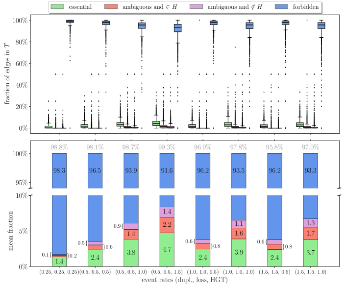
Figure 7: Classification of edges in the gene trees $T$ based on the true undirected Fitch graph (represented by the partition $\mathcal{P}$). The tuples on the horizontal axis give the rates for duplication, loss, and HGT events. Top panel: Fractions of four classes of edges: essential edges, ambiguous edges that are contained in $H$, ambiguous edges that are not contained in $H$, and forbidden edges. Lower panel: Mean values of the fractions of the four classes. The gray numbers are the proportions of scenarios (out of 5000 per rate combination) that were included in this analysis, i.e., the ones with $|L|>1$.

We also classified all ordered pairs $(x,y)$ with $x\in A$ and $y\in B$ in distinct sets $A,B\in\mathcal{P}$ as either essential, forbidden, or ambiguous (in analogy to the respective classification of $(A,B)$). Since the true directed Fitch graph $\digamma(T,H)$ is also known in the simulations, we can all determine for all ambiguous pairs $(x,y)$ whether they are present or absent in $\digamma(T,H)$. Fig. 8 summarizes the results of this edge classification.

Figure 8: Inference of edge orientation in the Fitch graphs of simulated scenarios on the basis of the true gene trees $T$ and the true undirected Fitch graph (represented by the partition $\mathcal{P}$). The tuples on the horizontal axis give the rates for duplication, loss, and HGT events. Top panel: The ordered gene pairs are divided into four classes, whose relative abundance is displayed: essential edges, forbidden edges, ambiguous edges that are present (p) in true directed Fitch graph, and ambiguous edges that are absent from true directed Fitch graph. Lower panel: Mean values of the fractions of the four classes. The gray numbers are the proportions of scenarios (out of 5000 per rate combination) that were included in the analysis, i.e., the ones with $|\mathcal{P}|>1$.

The upper panel shows the distributions of the abundances of essential, forbidden, and ambiguous edges as boxplots. These relative values were computed w.r.t. to the total number of pairs $(x,y)$ with $x$ and $y$ in distinct sets of $\mathcal{P}$ in each scenario. Simulated GFHs without HGT events (i.e., $|\mathcal{P}|=1$, $H=\emptyset$, and thus edge-less Fitch graphs) are excluded from the quantitative analysis. The fractions of GFHs with $|\mathcal{P}|>1$ are indicated by the gray percentage values in the lower panel of Fig. 8. The lower panel also contains the mean proportions of essential, forbidden, and ambiguous edges. To our surprise, $T$ and $\mathcal{P}$ unambiguously determine the presence or absence of an edge in the Fitch graph for 90-98% of the gene pairs $(x,y)$, depending on the rates of events.

The accuracy of gene trees is inherently limited due to the limited number of characters; collapsing poorly supported edges then results in minors of the true, fully resolved gene tree. Various sources of bias, furthermore, may result in incorrectly inferred topologies even with full bootstrap support, see e.g. (Hahn, 2007; Som, 2015) and the references therein. Several alternative approaches avoid the explicit reconstruction of a gene trees and instead directly leverage comparisons of similarities or distances to infer homology relations such as best matches and orthology (Setubal and Stadler, 2018; Altenhoff et al., 2019). Minors of gene trees can be obtained as “by-products” of orthology (Böcker and Dress, 1998; Hellmuth et al., 2013) or the best match relation (Geiß et al., 2019). Usually, these are not fully resolved, i.e., they can be obtained from the underlying true tree $T^{*}$ by a series of inner edge contractions. These trees contain partial but robust information about $T^{*}$. We consider here three distinct minors of $T^{*}$ that can be obtained in this manner: A unique discriminating cotree is associated with orthology relations (Hellmuth et al., 2013). Best-match relations uniquely determine the least-resolved tree (LRT), see (Geiß et al., 2019), and the binary-resolvable tree (BRT). A BRT exists whenever the underlying true gene tree $T^{*}$ was a binary tree (Schaller et al., 2021a), which is the case in our simulations. In this setting, our goal now is to classify pairs $(x,y)$ of genes as r-essential, r-forbidden, or r-ambiguous. Again we consider idealized conditions, i.e., we start from the true orthology and best match relations, which can be extracted directly from the simulated GFHs.

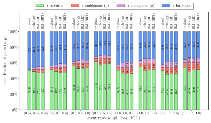
Figure 9: Inference of edge orientation in the Fitch graphs taking into account incomplete resolution of the trees. The same simulated scenarios as in Fig. 8 were included, and four trees were derived from them: the original gene tree (as in Fig. 8), the discriminating cotree of the orthology relation, as well as two trees obtained from best matches (BM). The plot shows mean values of the fractions of the four classes: r-essential edges, r-ambiguous edges that correspond to present (p) edges in the true directed Fitch graph, r-ambiguous edges that correspond to absent (a) edges, and r-forbidden edges.

Fig. 9 shows that the level of ambiguity remains surprisingly small when these minors of $T$ obtained from orthology and best matches are considered instead of the original, fully resolved tree. On average, the vast majority of pairs are still classified as r-essential and r-forbidden. We note that, for binary trees, essential and r-essential are equivalent. The same holds for forbidden and ambiguous explaining the identical values in Fig. 8 (lower panel) and Fig. 9 (original).

8 Concluding Remarks

Given a partition $\mathcal{P}$ of $L$ and a tree $T$ with leaf set $L$ that are compatible or at least r-compatible, we have obtained a complete characterization of the essential, forbidden, and ambiguous pairs $(A,B)$ of distinct sets $A,B\in\mathcal{P}$. Furthermore, we have shown that this classification can be computed in $O(|L|+|\mathcal{P}|^{2})$ time for given $T$ and $\mathcal{P}$. In biological terms, our result answers the question to what extent the direction of horizontal gene transfers between transfer-free subsets of genes (i.e., the sets of $\mathcal{P}$) are already determined by a (not necessarily fully resolved) gene tree $T$: If $(A,B)$ is essential, then for every $a\in A$ and $b\in B$, there is an HGT event between $\operatorname{lca}(a,b)$ and $b$; if $(A,B)$ is forbidden, no such HGT event can have taken place. In the ambiguous case, there are evolutionary scenarios of both types. This classification is of practical interest because the partition $\mathcal{P}$ of the gene set $L$ into HGT-free subsets, i.e., the undirected (symmetrized) Fitch graph, can be inferred from data (Schaller et al., 2021b), but so far no method has become available to directly obtain the (directed) Fitch graph from sequence or distance data. The mathematical results reported here thus provide a means of locating HGT events on the gene tree and at the same time to identify the ambiguities inherent in such a reconstruction.

From simulations of GFHs, we found that ambiguous edges are surprisingly rare in Fitch graphs. As expected for randomly generated HGT events, roughly half of the gene pairs are essential edges in the Fitch graph, while the other half are forbidden pairs. Only a few percent of the pairs are ambiguous. Regarding the edges in the gene tree, HGT can be ruled out for most of them. Still, the majority of potential HGT edges are essential, but the number of ambiguous edges is a sizeable fraction of $H^{*}$. The results are qualitatively similar for the fully resolved gene tree and several minors that can be inferred from orthology relations or best match relations. These numerical results indicate that HGT events can be identified fairly accurately from $T$ and $\mathcal{P}$. It therefore appears worthwhile to develop data analysis pipelines based on the results obtained here.

Still, a subset of the HGT events remains ambiguous in general. This begs the question whether there are additional sources of information that could be employed to further reduce the ambiguities. Several avenues to improve the resolution are conceivable. First, one may ask whether the LDT graph, which captures the experimental evidence more directly than the undirected Fitch graph or its system of independent sets $\mathcal{P}$, can be related directly to $T$. The LDT graph is always a cograph and hence associated with a discriminating cotree $T^{*}$. However, this cotree $T^{*}$ is not necessarily displayed by the true gene tree (Schaller et al., 2021b). Can one utilize the incompatibility of $T$ and $T^{*}$?

In practical applications, one usually also knows, for every $x\in L$, from which species $\sigma(x)$ the gene was obtained. This coloring induces additional constraints on the presence of HGT edges. For example, if two distinct sets $A,B\in\mathcal{P}$ contain elements with same the vertex color, i.e., if $\sigma(A)\cap\sigma(B)\neq\emptyset$, then there must be at least two HGT edges on the path between $\operatorname{lca}(A)$ and $\operatorname{lca}(B)$. Can one utilize this coloring information, which is also inherent in the LDT graphs, in a systematic manner? The observation of Hellmuth and Seemann (2019) that Fitch graphs determine certain rooted triples that are necessarily displayed by species tree suggests that this should indeed be possible.

Finally, throughout this contribution we have assumed that $\mathcal{P}$ is known but $T$ may be insufficiently resolved. What can be said if our knowledge of $\mathcal{P}$ contains errors? It is always possible to make $T$ and $\mathcal{P}$ compatible by refining $\mathcal{P}$ or coarsening $\mathcal{P}$, since every tree $T$ is compatible with both the discrete and the indiscrete partition, i.e., with $\{\{x\}\mid x\in L\}$ and $\{L\}$, respectively. In the first case, we have $H^{*}=E(T)$, in the second case $H^{*}=\emptyset$. What are the coarsest refinements and the finest coarsenings of $\mathcal{P}$ that are compatible with $T$? What can be said about the editing problem, if we assume that both $T$ and $\mathcal{P}$ contain errors?

Appendix A Additional Figures

Figures 8 and 9 show the fractions of (r-)essential, (r-)forbidden, and (r-)ambiguous pairs of genes $(x,y)$ in Fitch graphs for simulated (r-)compatible trees and partitions. In this appendix, we display the same data for the pairs of sets $(A,B)$ in the quotient Fitch graph. The relative abundances in Fig. 10 and Fig. 11, resp., are qualitatively very similar, indicating that biases such as imbalanced sizes of the sets $A$ and $B$ have little impact on the overall conclusion that ambiguity is relatively rare plausible GFHs.

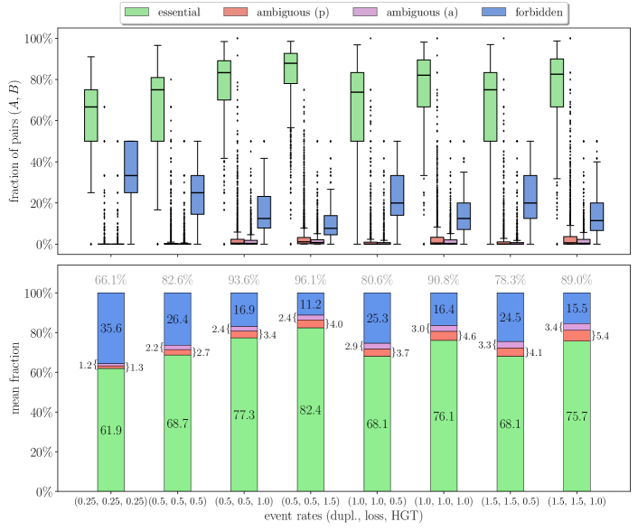
Figure 10: Inference of edge orientation in the Fitch quotient graphs of simulated scenarios. Top panel: Relative abundance of ordered pairs $(A,B)$ with $A,B\in\mathcal{P}$ that are essential, forbidden, ambiguous and present (p) in true Fitch quotient graph, and ambiguous and absent from true Fitch quotient graph. Lower panel: Mean values of the fractions of the four classes. See also the caption of the analogous Fig. 8.

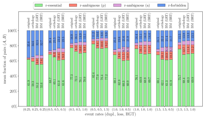
Figure 11: Inference of edge orientation in the Fitch quotient graphs taking into account incomplete resolution of the trees. The plot shows mean values of the fractions of pairs $(A,B)$ with $A,B\in\mathcal{P}$ that are r-essential, r-ambiguous and present (p) in the true Fitch quotient graph, r-ambiguous and absent (a), and r-forbidden. See also the caption of the analogous Fig. 9.

References

Altenhoff et al. (2019)
A. M. Altenhoff, N. M. Glover, and C. Dessimoz.
Inferring orthology and paralogy.
In M. Anisimova, editor, Evolutionary Genomics, volume 1910 of
Methods Mol. Biol. Humana, New York, NY, 2019.
doi: 10.1007/978-1-4939-9074-0˙5.
Bender and Farach-Colton (2004)
M. A. Bender and M. Farach-Colton.
The level ancestor problem simplified.
Theor. Comput. Sci., 321(1):5–12, 2004.
doi: 10.1016/j.tcs.2003.05.002.
Bender et al. (2005)
M. A. Bender, M. Farach-Colton, G. Pemmasani, S. Skiena, and P. Sumazin.
Lowest common ancestors in trees and directed acyclic graphs.
J. Algorithms, 57(2):75–94, 2005.
doi: 10.1016/j.jalgor.2005.08.001.
Berkman and Vishkin (1994)
O. Berkman and U. Vishkin.
Finding level-ancestors in trees.
J. Comput. Syst. Sci., 48(2):214–230,
1994.
doi: 10.1016/S0022-0000(05)80002-9.
Böcker and Dress (1998)
S. Böcker and A. W. M. Dress.
Recovering symbolically dated, rooted trees from symbolic
ultrametrics.
Adv. Math., 138:105–125, 1998.
doi: 10.1006/aima.1998.1743.
Fitch (2000)
W. M. Fitch.
Homology: a personal view on some of the problems.
Trends Genet., 16:227–231, 2000.
doi: 10.1016/S0168-9525(00)02005-9.
Geiß et al. (2018)
M. Geiß, J. Anders, P. F. Stadler, N. Wieseke, and M. Hellmuth.
Reconstructing gene trees from Fitch’s xenology relation.
J. Math. Biol., 77:1459–1491, 2018.
doi: 10.1007/s00285-018-1260-8.
Geiß et al. (2019)
M. Geiß, E. Chávez, M. González Laffitte, A. López Sánchez,
B. M. R. Stadler, D. I. Valdivia, M. Hellmuth, M. Hernández Rosales, and
P. F. Stadler.
Best match graphs.
J. Math. Biol., 78:2015–2057, 2019.
doi: 10.1007/s00285-019-01332-9.
Hahn (2007)
M. W. Hahn.
Bias in phylogenetic tree reconciliation methods: implications for
vertebrate genome evolution.
Genome Biol., 8:R141, 2007.
doi: 10.1186/gb-2007-8-7-r141.
Hellmuth (2017)
M. Hellmuth.
Biologically feasible gene trees, reconciliation maps and informative
triples.
Alg. Mol. Biol., 12(23), 2017.
doi: 10.1186/s13015-017-0114-z.
Hellmuth and Seemann (2019)
M. Hellmuth and C. R. Seemann.
Alternative characterizations of Fitch’s xenology relation.
J. Math. Biol., 79:969–986, 2019.
doi: 10.1007/s00285-019-01384-x.
Hellmuth and Wieseke (2016)
M. Hellmuth and N. Wieseke.
From sequence data incl. orthologs, paralogs, and xenologs to gene
and species trees.
In P. Pontarotti, editor, Evolutionary Biology – Convergent
Evolution, Evolution of Complex Traits, Concepts and Methods, pages
373–392, Cham, 2016. Springer.
doi: 10.1007/978-3-319-41324-2˙21.
Hellmuth et al. (2013)
M. Hellmuth, M. Hernandez-Rosales, K. T. Huber, V. Moulton, P. F. Stadler, and
N. Wieseke.
Orthology relations, symbolic ultrametrics, and cographs.
J. Math. Biol., 66:399–420, 2013.
doi: 10.1007/s00285-012-0525-x.
Hellmuth et al. (2015)
M. Hellmuth, N. Wieseke, M. Lechner, H.-P. Lenhof, M. Middendorf, and P. F.
Stadler.
Phylogenetics from paralogs.
Proc. Natl. Acad. Sci. USA, 112:2058–2063, 2015.
doi: 10.1073/pnas.1412770112.
Hellmuth et al. (2018)
M. Hellmuth, Y. Long, M. Geiß, and P. F. Stadler.
A short note on undirected Fitch graphs.
Art Discr. Appl. Math., 1:P1.08, 2018.
doi: 10.26493/2590-9770.1245.98c.
Hellmuth et al. (2021a)
M. Hellmuth, M. Michel, N. N. Nøjgaard, D. Schaller, and P. F. Stadler.
Combining orthology and xenology data in a common phylogenetic tree.
In P. F. Stadler, M. E. M. T. Walter, M. Hernandez-Rosales, and M. M.
Brigido, editors, Advances in Bioinformatics and Computational
Biology, volume 13063 of Lect. Notes Comp. Sci., pages 53–64, Cham,
CH, 2021a. Springer Nature.
doi: 10.1007/978-3-030-91814-9˙5.