Non-Sturmian sequences of matrices providing the maximum growth rate of matrix products

Abstract.

In the theory of linear switching systems with discrete time, as in other areas of mathematics, the problem of studying the growth rate of the norms of all possible matrix products $A_{\sigma_{n}}\cdots A_{\sigma_{0}}$ with factors from a set of matrices $\mathscr{A}$ arises. So far, only for a relatively small number of classes of matrices $\mathscr{A}$ has it been possible to accurately describe the sequences of matrices that guarantee the maximum rate of increase of the corresponding norms. Moreover, in almost all cases studied theoretically, the index sequences $\{\sigma_{n}\}$ of matrices maximizing the norms of the corresponding matrix products have been shown to be periodic or so-called Sturmian, which entails a whole set of “good” properties of the sequences $\{A_{\sigma_{n}}\}$, in particular the existence of a limiting frequency of occurrence of each matrix factor $A_{i}\in\mathscr{A}$ in them. In the paper it is shown that this is not always the case: a class of matrices is defined consisting of two $2\times 2$ matrices, similar to rotations in the plane, in which the sequence $\{A_{\sigma_{n}}\}$ maximizing the growth rate of the norms $\|A_{\sigma_{n}}\cdots A_{\sigma_{0}}\|$ is not Sturmian. All considerations are based on numerical modeling and cannot be considered mathematically rigorous in this part; rather, they should be interpreted as a set of questions for further comprehensive theoretical analysis.

1. Introduction

Various problems of mathematics reduce to the problem of computing the maximum growth rate of the norms of matrix products $A_{\sigma_{n}}\cdots A_{\sigma_{0}}$ with factors from a set of matrices $\mathscr{A}$.

One of the basic, though greatly simplified, examples of this type of situation is found in systems and control theory (Brayton and Tong, 1979; Blondel and Tsitsiklis, 2000; Blondel and Canterini, 2003; Shorten et al., 2007; Jungers, 2009; Wu and He, 2020) when considering the asymptotic behavior of solutions of the so-called linear switching system with discrete time, whose dynamics is described by the equation

$$x_{n+1}=A_{\sigma_{n}}x_{n},\qquad\sigma_{n}\in\{0,1,\ldots,m-1\},\leavevmode\nobreak\ n\geq 0,$$ (1)

where $A_{\sigma_{i}}\in\mathscr{A}:=\{A_{0},A_{1},\ldots,A_{m-1}\}$. The solutions for system (1) may be represented as follows:

$$x_{n}=A_{\sigma_{n-1}}\cdots A_{\sigma_{1}}A_{\sigma_{0}}x_{0}.$$ (2)

Therefore, in studying the question of their asymptotic behavior, we naturally come to the problem of estimating (and preferably computing exactly) the growth rate of the norms $\|A_{\sigma_{n}}\cdots A_{\sigma_{1}}A_{\sigma_{0}}\|$ with arbitrary factors $A_{\sigma_{i}}\in\mathscr{A}$. Of course, the set of questions related to the analysis of the asymptotic behavior of $x_{n}$ elements can be extended, but in this paper we will not deal with such generalizations.

It is worth noting that the problem of computing the maximum possible growth rate of the norms of matrix products with factors from a set of matrices is quite general; in particular, numerous problems in other areas of science are reduced to it, for example, in coding theory (Moision et al., 2001; Blondel et al., 2006), computational mathematics (Daubechies and Lagarias, 1992; Heil and Strang, 1995; Maesumi, 1998; Daubechies and Lagarias, 2001; Jungers et al., 2008), and the theory of parallel and distributed computation (Chazan and Miranker, 1969; Bertsekas and Tsitsiklis, 1989).

Currently, the range of questions related to the analysis of the growth rate of the norms of matrix products $A_{\sigma_{n}}\cdots A_{\sigma_{1}}A_{\sigma_{0}}$ is usually considered in the framework of the so-called theory of joint/generalized spectral radius, which emerged in the 1960s (Rota and Strang, 1960; Daubechies and Lagarias, 1992; Lagarias and Wang, 1995; Daubechies and Lagarias, 2001) and now has several hundred publications (Kozyakin, 2013a). Moreover, in almost all cases studied theoretically, the index sequences $\{\sigma_{n}\}$ of matrices maximizing the norms of the corresponding matrix products turned out to be periodic or so-called Sturmian. Both the periodicity and the fact that the index sequences $\{\sigma_{n}\}$ are Sturmian entail a whole set of “good” properties of the sequences $\{A_{\sigma_{n}}\}$, in particular the existence of a limiting frequency of occurrence of each matrix factor $A_{i}\in\mathscr{A}$ (Bousch and Mairesse, 2002; Blondel et al., 2003; Kozyakin, 2005a, 2007).

This may give the false impression that periodic or Sturmian sequences occur every time one tries to maximize the norms of matrix products (at least in the case of a pair of ${2\times 2}$ matrices). This impression is reinforced by the fact that we are not aware of any theoretical studies in this area, apart from those leading to the appearance of periodic or Sturmian sequences, which can be explained by the extreme theoretical and technical complexity of the corresponding analysis. The aim of this paper is to refute this impression. To this end, we determine a class of ${2\times 2}$ matrices consisting of two matrices similar to rotations of the plane in which the sequence $\{A_{\sigma_{n}}\}$ maximizing the growth rate of the norms $\|A_{\sigma_{n}}\cdots A_{\sigma_{0}}\|$ is not Sturmian.

Let us describe the structure of the work. The introduction provides a rationale for the topics covered here. Section 2 briefly recalls the main facts and constructions from the theory of joint/generalized spectral radius, among which . ‣ Theoretical Background plays a crucial role. Section 3 recalls the concept of extremal trajectories, i.e., trajectories with the maximum rate of increase in a certain Barabanov norm. Here we describe a general approach which, in the case of a pair of ${2\times 2}$ matrices, reduces the problem of constructing extremal trajectories to the problem of studying iterations of a certain mapping of an interval into itself (or, equivalently, of a circle into itself) with a fairly simple structure. Section 4 recalls the well-known theoretical results on the construction and growth of extremal trajectories, which refer to the case of a pair of nonnegative ${2\times 2}$ matrices of a special form. This case underlies most modern studies of “nontrivial” situations in joint/generalized spectral radius theory. The above theoretical results are illustrated by examples of computer simulations. Section 5 considers the case of a pair of matrices, each of which is similar to a rotation matrix. Using the results of numerical simulations, it is shown that for such matrices a previously unobserved phenomenon occurs in which the index sequences of the extremal trajectories turn out to be non-Sturmian (. ‣ A Pair of Matrices Similar to Plane Rotations). For a description of the methods and means for numerical modeling of the behavior of matrix products used in this work, see Section 6.

2. Theoretical Background

Recall the basic concepts and results related to the theory of joint/generalized spectral radius, following (Kozyakin, 2005a, b, 2007).

Let $\mathscr{A}=\{A_{0},\ldots,A_{m-1}\}$ be a set of $m$ real $d\times d$ matrices, and $\|\cdot\|$ be some norm in ${\mathbb{R}}^{d}$. For every $n\geq 1$, with every finite sequence $\boldsymbol{\sigma}=\{\sigma_{0},\sigma_{1},\ldots,\sigma_{n-1}\}\in{\{0,\ldots,m-1\}}^{n}$ we link the matrix

$$A_{\boldsymbol{\sigma}}=A_{\sigma_{n-1}}\cdots A_{\sigma_{1}}A_{\sigma_{0}},$$

and define two numerical values:

$$\rho_{n}({\mathscr{A}})=\max_{\boldsymbol{\sigma}\in{\{0,\ldots,m-1\}}^{n}}\|A_{\boldsymbol{\sigma}}\|^{1/n},\qquad\bar{\rho}_{n}({\mathscr{A}})=\max_{\boldsymbol{\sigma}\in{\{0,\ldots,m-1\}}^{n}}{\rho(A_{\boldsymbol{\sigma}})}^{1/n},$$

where $\rho(\cdot)$ denotes the spectral radius of a matrix. In these designations, the limit

$$\rho({\mathscr{A}})=\limsup_{n\to\infty}\rho_{n}({\mathscr{A}}),$$

which does not depend on the choice of the norm $\|\cdot\|$ (and in fact coincides with the limit $\rho({\mathscr{A}})=\lim_{n\to\infty}\rho_{n}({\mathscr{A}})$) is called the joint spectral radius of the set of matrices $\mathscr{A}$ (Rota and Strang, 1960). Similarly, we can consider the limit

$$\bar{\rho}({\mathscr{A}})=\limsup_{n\to\infty}\bar{\rho}_{n}({\mathscr{A}}),$$

called the generalized spectral radius of the matrix set $\mathscr{A}$ (Daubechies and Lagarias, 1992). The values $\rho({\mathscr{A}})$ and $\bar{\rho}({\mathscr{A}})$ for bounded families of matrices $\mathscr{A}$ actually coincide with each other (Berger and Wang, 1992), and, moreover, for any $n$, the following inequalities hold:

$$\bar{\rho}_{n}({\mathscr{A}})\leq\bar{\rho}({\mathscr{A}})=\rho({\mathscr{A}})\leq\rho_{n}({\mathscr{A}}).$$ (3)

It follows from the definition of the joint spectral radius that for each $\varepsilon>0$ the rate of growth of the norms $\|A_{\boldsymbol{\sigma}}\|=\|A_{\sigma_{n-1}}\cdots A_{\sigma_{1}}A_{\sigma_{0}}\|$ for large $n$ does not exceed ${(\rho({\mathscr{A}})+\varepsilon)}^{n}$, that is,

$$\|A_{\boldsymbol{\sigma}}\|=\|A_{\sigma_{n-1}}\cdots A_{\sigma_{1}}A_{\sigma_{0}}\|\leq{(\rho({\mathscr{A}})+\varepsilon)}^{n}$$ (4)

for each finite sequence of indices

$$\boldsymbol{\sigma}=\{\sigma_{0},\sigma_{1},\ldots,\sigma_{n-1}\}\in{\{0,\ldots,m-1\}}^{n}.$$

Moreover, there are arbitrarily large $n$ and sequences of indices $\boldsymbol{\sigma}$ for which

$$\rho(A_{\boldsymbol{\sigma}})=\rho(A_{\sigma_{n-1}}\cdots A_{\sigma_{1}}A_{\sigma_{0}})\geq{(\bar{\rho}({\mathscr{A}})-\varepsilon)}^{n},$$

and therefore, for such $n$, by virtue of (3), the inequalities

$$\|A_{\boldsymbol{\sigma}}\| =\|A_{\sigma_{n-1}}\cdots A_{\sigma_{1}}A_{\sigma_{0}}\|\geq$$

$$\geq\rho(A_{\sigma_{n-1}}\cdots A_{\sigma_{1}}A_{\sigma_{0}})\geq{(\bar{\rho}({\mathscr{A}})-\varepsilon)}^{n}\equiv{(\rho({\mathscr{A}})-\varepsilon)}^{n}$$ (5)

will hold.

Inequalities (4) and (5) raise at least two questions: first, is it possible to set $\varepsilon$ in them equal to zero, and second, if this is possible, how can we describe the sets of indices $\boldsymbol{\sigma}=\{\sigma_{0},\sigma_{1},\ldots,\sigma_{n-1}\}$, for which inequality (4) becomes an equality with $\varepsilon=0$?

The answer to the first question is negative; it follows from the following simple remark. Let the set $\mathscr{A}$ consist of one square matrix $A$. Then by the well-known Gelfand formula (Horn and Johnson, 1985, Corollary 5.6.14) both values $\rho({\mathscr{A}})$ and $\bar{\rho}({\mathscr{A}})$ coincide with the spectral radius $\rho(A)$ of the matrix $A$. In this case, by reducing the matrix $A$ to normal Jordan form, one can easily establish that the growth rate of the norms $\|A^{n}\|$ is of order ${\rho(A)}^{n}$ if and only if the eigenvalues of the matrix $A$ that have the largest absolute value are semisimple. At the same time, for the case when at least one such eigenvalue of the matrix $A$ is not semisimple, the growth rate of the norms $\|A^{n}\|$ is of order $p(n){\rho(A)}^{n}$, where $p(t)$ is a polynomial.

The answer to the first question has another nuance: Even in cases where the growth rate of the norms of the matrix products $\|A_{\sigma_{n-1}}\cdots A_{\sigma_{1}}A_{\sigma_{0}}\|$ for a particular choice of the sequence of indices $\{\sigma_{0},\sigma_{1},\ldots,\sigma_{n-1}\}\in{\{0,\ldots,m-1\}}^{n}$ may coincide with ${\rho(\mathscr{A})}^{n}$, this may not happen for all norms of $\|\cdot\|$ but only for a particular choice of the corresponding norm. Moreover, even in the case of sets of matrices $\mathscr{A}$ consisting of a single matrix, the construction of the corresponding norm turns out to be a nontrivial problem!

However, even in the simplest nontrivial case, when the set of matrices $\mathscr{A}$ consists of a pair of matrices of dimension ${2\times 2}$, the question posed turns out to be much more complicated than the analysis of the growth rate of the norms of degrees $\|A^{n}\|$ of one matrix $A$. More precisely, unlike the corresponding analysis for one matrix, in the general case the computation of the maximal growth rate of the norms $\|A_{\sigma_{n}}\cdots A_{\sigma_{1}}A_{\sigma_{0}}\|$ turns out to be algebraically impossible (Kozyakin, 1990, 2003, 2013b), and the approximate computation of the corresponding rate turns out to be NP-hard (Tsitsiklis and Blondel, 1997; Blondel and Tsitsiklis, 2000).

Nevertheless, in a fairly general situation, a theoretically satisfactory answer to the first question can still be obtained. Recall that a set of matrices $\mathscr{A}$ is called irreducible if matrices from $\mathscr{A}$ have no common invariant subspaces other than $\{0\}$ and ${\mathbb{R}}^{d}$. The irreducibility of a set of matrices plays the same role in studying the growth rate of the norms of matrix products with multiple matrix factors as the semisimplicity of the eigenvalues with the largest absolute value of a single matrix plays in studying the growth rate of the norms of its powers. The approach proposed by N. Barabanov in (Barabanov, 1988a, b, c) proved to be the most fruitful here, and it has been further developed in several papers, from which we single out (Wirth, 2002).

Barabanov’s Theorem.

If the set of matrices $\mathscr{A}=\{A_{0},\ldots,A_{m-1}\}$ is irreducible, then the number $\rho$ is the joint (generalized) spectral radius of the set $\mathscr{A}$ if and only if there exists a norm $\|\cdot\|$ in ${\mathbb{R}}^{d}$ such that

$$\rho\|x\|=\max\left\{\|A_{0}x\|,\|A_{1}x\|,\ldots,\|A_{m-1}x\|\right\},\qquad\forall\leavevmode\nobreak\ x\in\mathbb{R}^{d}.$$ (6)

A norm satisfying (6) is usually called the Barabanov norm corresponding to the set of matrices $\mathscr{A}$. This theorem does not provide a constructive description of Barabanov norms. Nevertheless, it turns out to be very effective in analyzing the growth of matrix products. In particular, it follows from . ‣ Theoretical Background that for irreducible sets of matrices $\mathscr{A}$, for every finite sequence of indices $\boldsymbol{\sigma}=\{\sigma_{0},\sigma_{1},\ldots,\sigma_{n-1}\}\in{\{0,\ldots,m-1\}}^{n}$, in the Barabanov norm the inequality

$$\|A_{\sigma_{n-1}}\cdots A_{\sigma_{1}}A_{\sigma_{0}}\|\leq{\rho({\mathscr{A}})}^{n}$$

holds, and that there is an infinite sequence of indices $\boldsymbol{\sigma}=\{\sigma_{0},\sigma_{1},\ldots\}$ such that for every $n$ the equality

$$\|A_{\sigma_{n-1}}\cdots A_{\sigma_{1}}A_{\sigma_{0}}\|={\rho({\mathscr{A}})}^{n}$$

holds. So for irreducible sets of matrices there are much stronger statements than inequalities (4) and (5).

The second question, how to describe sets of indices $\boldsymbol{\sigma}=\{\sigma_{0},\sigma_{1},\ldots,\sigma_{n-1}\}$, for which inequality (4) turns into equality when $\varepsilon=0$, is much more complicated than the first. The answer is currently known either in trivial (and therefore theoretically uninteresting) situations or in some special and rather restrictive cases. The answer to this question (as of the current understanding of the problem) is closely related to the concept of extremal trajectories of sets of matrices, which we briefly recall in the next section.

3. Extremal Trajectories

In stating the main facts of this section we shall, as in the preceding section, adhere to the works (Kozyakin, 2005a, b, 2007). Additional discussion of the problems and statements involved can also be found in (Jungers, 2009).

The question of the growth rate of matrix products with factors from a certain set of matrices $\mathscr{A}$ is closely related to a similar question of the growth rate of solutions of the difference equation (1) for all possible choices of index sequences $\{\sigma_{n}\}$ and initial values $x_{0}$. The solutions $\{x_{n}\}$ of equation (1) will also be called the trajectories defined by the set of matrices $\mathscr{A}$, or simply the trajectories of the set of matrices $\mathscr{A}$. Since, according to (2), each element $x_{n}$ of the trajectory $\{x_{n}\}$ can be represented as

$$x_{n}=A_{\sigma_{n-1}}\cdots A_{\sigma_{1}}A_{\sigma_{0}}x_{0},$$

then due to (4)

$$\|x_{n}\|\leq\|A_{\sigma_{n-1}}\cdots A_{\sigma_{1}}A_{\sigma_{0}}\|\,\|x_{0}\|\leq e^{(\rho({\mathscr{A}})+\varepsilon)n}\|x_{0}\|$$

for all sufficiently large $n$.

A trajectory $\{x_{n}\}$ of the set of matrices $\mathscr{A}$ was called characteristic in (Kozyakin, 2005a, b, 2007) if it satisfies the inequalities

$$c_{1}\rho^{n}(\mathscr{A})\leq\|x_{n}\|\leq c_{2}\rho^{n}(\mathscr{A}),\qquad n=0,1,2,\ldots\,,$$

for some choice of constants $c_{1},c_{2}\in(0,\infty)$. In other words, by characteristic trajectories are meant those trajectories which, in the natural sense, are uniformly comparable to the sequence $\{\rho^{n}(\mathscr{A})\}$ on the whole infinite interval $n=0,1,2,\ldots$ of the variation of their indices. Note that the definition of the characteristic trajectory does not depend on the choice of the norm $\|\cdot\|$ in the space $\mathbb{R}^{d}$.

An important special case of characteristic trajectories is the so-called extremal trajectories. A trajectory $\{x_{n}\}$ of a collection of matrices $\mathscr{A}$ will be called extremal if in some Barabanov norm $\|\cdot\|$ it satisfies the identity

$$\rho^{-n}(\mathscr{A})\|x_{n}\|\equiv\textrm{const}.$$ (7)

As mentioned in Section 2, there are Barabanov norms for any irreducible set of matrices. Then, for any irreducible set of matrices, there are also extremal trajectories and hence characteristic trajectories. For the proof, it suffices to construct the trajectory $\{x_{n}\}$ of the set of matrices $\mathscr{A}=\{A_{0},\ldots,A_{m-1}\}$, satisfying the initial condition $x_{0}=x$, recursively. Let the element $x_{n}$ have already been formed. Then, according to the definition of the Barabanov norm, the equality

$$\rho(\mathscr{A})\|x_{n}\|=\max\left\{\|A_{0}x_{n}\|,\|A_{1}x_{n}\|,\ldots,\|A_{m-1}x_{n}\|\right\}$$

holds. Therefore, there exists an index $\sigma_{n}$ such that

$$\rho(\mathscr{A})\|x_{n}\|=\|A_{\sigma_{n}}x_{n}\|,$$

and for condition (7) to be satisfied, it suffices to define the element $x_{n+1}$ by the equality $x_{n+1}=A_{\sigma_{n}}x_{n}$.

Unlike the definition of a characteristic trajectory, the definition of an extremal trajectory depends on the choice of an extremal norm: A trajectory that is extremal in one norm may not be extremal in another norm. Nevertheless, for an irreducible set of matrices, there are always universal extremal trajectories in a certain sense, i.e., trajectories which are extremal with respect to any extremal norm: As shown in (Kozyakin, 2007, Th. 3), every limit point of every normed characteristic trajectory $\{x_{n}/\|x_{n}\|\}$ serves as the initial value of a trajectory which is automatically extremal in every Barabanov norm.

The description of extremal trajectories includes, besides the sequence $\boldsymbol{x}=\{x_{n}\}$, the index sequence $\{\sigma_{n}\}$, which is used to obtain the trajectory $\{x_{n}\}$ according to (1). In the following, we describe a construction that allows to define extremal trajectories as all possible trajectories of a multivalued nonlinear dynamical system, thus dispensing with the explicit description of the index sequence $\{\sigma_{n}\}$.

Let $\rho=\rho(\mathscr{A})$, and let $\|\cdot\|$ be a Barabanov norm corresponding to the set of matrices $\mathscr{A}=\{A_{0},\ldots,A_{m-1}\}$. For each $x\in\mathbb{R}^{d}$, we define the mapping $g(x)$ by

$$g(x):=\{w:\leavevmode\nobreak\ \exists i\in\{0,\ldots,m-1\}:\leavevmode\nobreak\ w=A_{i}x,\textrm{\leavevmode\nobreak\ where\leavevmode\nobreak\ }\|A_{i}x\|=\rho\|x\|\}.$$ (8)

By the definition of the Barabanov norm, for any ${x\in\mathbb{R}^{d}}$, the set $g(x)$ is nonempty and consists of at most $m$ elements. Note that every mapping $g(x)$ has a closed graph and the identity

$$\|g(x)\|\equiv\rho\|x\|$$ (9)

holds for it.

Clearly, the sequence $\boldsymbol{x}=\{x_{n}\}$ is an extremal trajectory of the set of matrices $\mathscr{A}$ in the Barabanov norm $\|\cdot\|$ if and only if it satisfies the inclusions

$$x_{n+1}\in g(x_{n}),\qquad\forall\leavevmode\nobreak\ n.$$

In other words, every trajectory of the multivalued mapping $g(\cdot)$ turns out to be an extremal trajectory of the set of matrices $\mathscr{A}$ in the Barabanov norm $\|\cdot\|$. This gives rise to call the map $g(\cdot)$ a generator of extremal trajectories. Just like the Barabanov norm, the map $g(\cdot)$ cannot be stated explicitly in the general case. Nevertheless, a rather detailed description of the properties of generators of extremal trajectories can be obtained for two-element (i.e., $m=2$) sets of nonnegative ${2\times 2}$ matrices. Let us describe the corresponding constructions in detail.

We fix in space $\mathbb{R}^{2}$ a Barabanov norm $\|\cdot\|$ corresponding to the set of matrices $\mathscr{A}=\{A_{0},A_{1}\}$. Let us define the sets

$$X_{0}=\{x:\leavevmode\nobreak\ \|A_{0}x\|=\rho\|x\|\},\qquad X_{1}=\{x:\leavevmode\nobreak\ \|A_{1}x\|=\rho\|x\|\}.$$ (10)

Each of these sets is closed, conic (i.e., it contains, together with the vector $x\neq 0$, each vector of the form $tx$, where $t\geq 0$), and by the definition of the Barabanov norm $X_{0}\cup X_{1}={\mathbb{R}}^{2}$. In this case, the generator of extremal trajectories $g(\cdot)$ (see (8)) in the norm $\|\cdot\|$ takes the form

$$g(x)=\left\{\begin{array}[]{cl}A_{0}x&\textrm{for\leavevmode\nobreak\ }x\in X_{0}\backslash X_{1},\\ A_{1}x&\textrm{for\leavevmode\nobreak\ }x\in X_{1}\backslash X_{0},\\ \{A_{0}x,A_{1}x\}&\textrm{for\leavevmode\nobreak\ }x\in X_{0}\cap X_{1}.\end{array}\right.$$ (11)

Let us examine more closely the structure of the mapping $g(\cdot)$. Let $(r,\varphi)$ be the polar coordinates of the vector $x\in\mathbb{R}^{2}$. We denote by $\Omega_{0}$ and $\Omega_{1}$ the angular projections of the conic sets $X_{0}$ and $X_{1}$, respectively. As mentioned above (see (9)), the mapping $g(\cdot)$ satisfies the identity $\|g(x)\|\equiv\|x\|$. Thus, in the polar coordinate system $(r,\varphi)$, the mapping $g$ has the form of a mapping with separable variables

$$g:(r,\varphi)\mapsto(\rho r,\varPhi(\varphi)),$$ (12)

where $\rho=\rho(\mathscr{A})$ and

$$\varPhi(\varphi)=\left\{\begin{array}[]{cl}\varPhi_{0}(\varphi)&\textrm{for\leavevmode\nobreak\ }\varphi\in\Omega_{0},\\ \varPhi_{1}(\varphi)&\textrm{for\leavevmode\nobreak\ }\varphi\in\Omega_{1},\\ \{\varPhi_{0}(\theta),\varPhi_{1}(\theta)\}&\textrm{for\leavevmode\nobreak\ }\varphi\in\Omega_{0}\cap\Omega_{1}.\end{array}\right.$$ (13)

Here the functions $\varPhi_{0}(\varphi)$ and $\varPhi_{1}(\varphi)$ are explicitly defined as the angular coordinates of the mappings $A_{0}x$ and $A_{1}x$, when $x=(r,\varphi)$ in polar coordinates.

The angular coordinate $\varphi$ characterizes the direction of the vector $x=(r,\varphi)$. Accordingly, it is natural to interpret $\varPhi(\varphi)$, $\varphi\in[0,2\pi)$, as a direction function or angular function of the generator of extremal trajectories $g(\cdot)$. Note also that the function $\varPhi(\varphi)$, while $2\pi$-periodic, is in general not continuous. And since it is obtained as a result of taking the angular coordinates of linear mappings, its value modulo $\pi$, the function

$$\tilde{\varPhi}(\varphi)=\varPhi(\varphi)\bmod\pi,\qquad\varphi\in[0,\pi),$$ (14)

is a $\pi$-periodic function.

From the definition (8) of the function $g(\cdot)$ and its representation in the form (12) we obtain the following description of extremal trajectories (Kozyakin, 2007, Lemma 6).

Lemma 1.

The nonzero trajectory $\{x_{n}\}$ is extremal for the set of ${{2\times 2}}$ matrices $\mathscr{A}=\{A_{0},A_{1}\}$ in the Barabanov norm $\|\cdot\|$ if and only if its elements in the polar coordinate system $(r,\varphi)$ are representable as $x_{n}=(\rho^{n}r_{0},\varphi_{n})$, where $\rho$ is the joint/generalized spectral radius of the set of matrices $\mathscr{A}$, and $\{\varphi_{n}\}$ is the trajectory of the multivalued mapping $\varPhi(\cdot)$, i.e.

$$\varphi_{n+1}\in\varPhi(\varphi_{n}),\qquad n=0,1,\ldots\leavevmode\nobreak\ .$$

Moreover, the trajectory $\{x_{n}\}$ satisfies the equations

$$x_{n+1}=A_{\sigma_{n}}x_{n},\qquad n=0,1,\ldots\leavevmode\nobreak\ ,$$

with some index sequence $\{\sigma_{n}\}$ if and only if the trajectory $\{\varphi_{n}\}$ satisfies the equations

$$\varphi_{n+1}=\varPhi_{\sigma_{n}}(\varphi_{n}),\qquad n=0,1,\ldots\leavevmode\nobreak\ ,$$

or, which is equivalent, when the trajectory $\{\tilde{\varphi}_{n}\}$ with elements

$$\tilde{\varphi}_{n}=\varphi_{n}\bmod\pi,\qquad n=0,1,\ldots\leavevmode\nobreak\ ,$$

satisfies the equations

$$\tilde{\varphi}_{n+1}=\tilde{\varPhi}_{\sigma_{n}}(\tilde{\varphi}),\qquad n=0,1,\ldots\leavevmode\nobreak\ .$$

4. A Pair of Nonnegative Matrices

Despite the fact that the Barabanov norm $\|\cdot\|$ is, as a rule, not known explicitly, the angular function $\varPhi(\varphi)$ of the generator of extremal trajectories $g(\cdot)$ turns out in some cases to be defined “unambiguous enough.” In this context, we recall some constructions and results from (Kozyakin, 2005b, 2007) developed to construct one of the counterexamples to the so-called Finiteness Conjecture (Lagarias and Wang, 1995; Bousch and Mairesse, 2002; Blondel et al., 2003).

Consider the set of matrices $\mathscr{A}=\{A_{0},A_{1}\}$, where

$$A_{0}=\alpha\left[\begin{array}[]{cc}a&b\\ 0&1\end{array}\right],\quad A_{1}=\beta\left[\begin{array}[]{cc}1&0\\ c&d\end{array}\right].$$ (15)

For this set of matrices in (Kozyakin, 2005b, 2007) it was possible to perform a detailed analysis of the structure of the extremal trajectories under the additional assumptions that $\alpha,\beta>0$ and

$$bc\geq 1\geq a,d>0.$$

In this paper, the approximate construction of the Barabanov norms of the sets of the matrix sets (15) (and the visualization of their unit spheres) were carried out using the algorithms and programs described in Section 6. An example of the unit sphere of the Barabanov norm for the set of matrices (15), one of the extremal trajectories, and the corresponding angular function $\tilde{\varPhi}(\varphi)$ for the case

$$\alpha=0.576,\quad\beta=0.8,\quad a=d=0.9,\quad b=1.1,\quad c=1,$$ (16)

is shown in Fig. 1(a). Here the black solid line represents the unit sphere of the Barabanov norm, i.e., the set of points $x\in\mathbb{R}^{2}$ for which $\|x\|=1$ holds. Dotted and dashed lines denote the sets of points $x\in\mathbb{R}^{2}$ for which $\|A_{0}x\|=\rho$ and $\|A_{1}x\|=\rho$, respectively, where $\rho=\rho(\mathscr{A})$ is the joint/generalized spectral radius of the matrix set $\mathscr{A}$. Dash-dotted lines denote straight lines consisting of points $x\in X_{0}\cap X_{1}$ (see (10)), i.e., points satisfying the equality $\|A_{0}x\|=\|A_{1}x\|$. Figure 1(b) shows the trajectory with the maximum rate of increase of the Barabanov norm $\|\cdot\|$. The construction of the next point of the trajectory $x_{n+1}$ depends on which of the sectors bounded by straight dash-dotted lines the point $x_{n}$ belongs to; the type of matrix used for this, $A_{0}$ or $A_{1}$, is indicated in the shaded areas of Fig. 1(b). The numerical analysis performed shows that $\rho(\mathscr{A})\approx 1.098668$ and the index sequence $\{\sigma_{n}\}$ of the extremal trajectory shown in Fig. 1(b) is of the form

$$\{\sigma_{n}\}=10110110101101101101011011011010110110110101101101\ldots\,,$$ (17)

where on sufficiently large segments (words) of the sequence $\{\sigma_{n}\}$ of length $10000$ the symbol $\boldsymbol{0}$ occurs with a frequency of $\approx 0.364$ and the symbol $\boldsymbol{1}$ occurs with a frequency of $\approx 0.636$. The index sequence $\{\sigma_{n}\}$ was constructed with the program barnorm_sturm.py by computing point iterations using the angular function $\tilde{\varPhi}(\varphi)$, as shown in Figs. 1(c) and 2. In these figures, the thick solid lines denote sections of the graphs of the functions $\varPhi_{0}(\varphi)$ and $\varPhi_{1}(\varphi)$ through which, according to (13)–(14) the function $\tilde{\varPhi}(\varphi)$ is determined, and thin dashed lines mark those sections of the graphs of the functions $\varPhi_{0}(\varphi)$ and $\varPhi_{1}(\varphi)$ that were discarded in the definition of the function $\tilde{\varPhi}(\varphi)$.

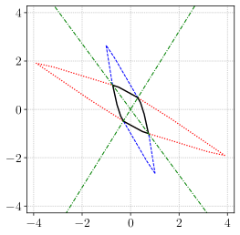
(a) A Barabanov norm

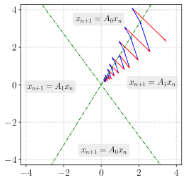
(b) A maximum growth rate trajectory

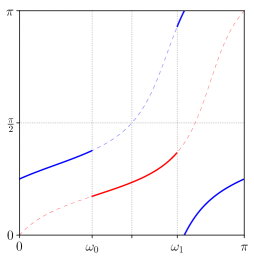
(c) The function $\tilde{\varPhi}(\varphi)$ preserves orientation and has two discontinuity points

Figure 1. A Barabanov norm and the angular function for the set of matrices (15), where $\alpha=0.576$, $\beta=0.8$, $a=d=0.9$, $b=1.1$, $c=1$

In this case, the fact that both matrices $A_{0}$ and $A_{1}$ are nonnegative and therefore leave the first quadrant in $\mathbb{R}^{2}$ invariant proved to be of fundamental importance for the theoretical study of the structure of extremal trajectories carried out in (Kozyakin, 2005b, 2007). The latter fact is reflected in the observation that the angular function $\tilde{\varPhi}(\varphi)$ in this case maps the segment $\left[0,\frac{\pi}{2}\right)$ into itself, which simplifies the study of its trajectories $\{\tilde{\varphi}_{n}\}$. In particular, it was proved in (Kozyakin, 2005b, 2007) that the restrictions of the sets $\Omega_{0}$ and $\Omega_{1}$ in (13) on $\left[0,\frac{\pi}{2}\right)$ are segments with a single common point $\omega_{0}$. As numerical calculations show, in the case (16) we are considering, these sets are as follows:

$$\textstyle\Omega_{0}\cap\left[0,\frac{\pi}{2}\right)=\left[\omega_{0},\frac{\pi}{2}\right),\quad\Omega_{1}\cap\left[0,\frac{\pi}{2}\right)=\left[0,\omega_{0}\right).$$

Accordingly, the function $\tilde{\varPhi}(\varphi)$ in our case has only one discontinuity point $\omega_{0}$ on the segment $\left[0,\frac{\pi}{2}\right)$, see Fig. 2.

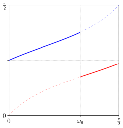
Figure 2. The angular function $\tilde{\varPhi}(\varphi)$, $\varphi\in\left[0,\frac{\pi}{2}\right)$, for the set of matrices (15)

If we treat $\varphi\in\left[0,\frac{\pi}{2}\right)$ as an angular coordinate on a circle of length $\frac{\pi}{2}$, we can take $\tilde{\varPhi}(\varphi)$ as an orientation-preserving mapping of the corresponding circle into itself, see (Kozyakin, 2005b, 2007) for details. In this case, as shown in (Kozyakin, 2005b, 2007), the index sequence $\{\sigma_{n}\}$ of each trajectory $\tilde{\varphi}_{n}$ of the mapping $\tilde{\varPhi}$ turns out to be either periodic or the so-called Sturmian (see, e.g., (Fogg, 2002, Ch. 6), (Lothaire, 2002, Ch. 2)).

Currently, there are several definitions of the Sturmian sequences. One of the simplest analytic definitions states that a Sturmian sequence is an integer sequence $\{\sigma_{n}\}$, which for all integer $n$ is defined by the relations

$$\sigma_{n}=[(n+1)\theta+\eta]-[n\theta+\eta],$$

where $\theta\in(0,1)$ is an irrational number, $\eta\in\mathbb{R}$, and $[\cdot]$ denotes the integer part of the number. The following equivalent definition will be more useful for us: let $\{\varphi_{n}\}$ be a trajectory running on a circle of length $1$ (or, equivalently, on the interval $[0,1)$) through the rotation map

$$\varphi_{n+1}=\varphi_{n}+\theta\bmod 1,$$ (18)

where $\theta$ is an irrational number. We associate the index sequence $\{\sigma_{n}\}$ with this trajectory and set (see Fig. 3(a))

$$\sigma_{n}=\begin{cases}0,&\text{if\leavevmode\nobreak\ }\varphi_{n}\in I_{0}:=[\theta,1),\\ 1,&\text{if\leavevmode\nobreak\ }\varphi_{n}\in I_{1}:=[0,\theta).\end{cases}$$ (19)

Then the resulting sequence $\boldsymbol{\sigma}=\{\sigma_{n}\}$ (which is not periodic due to the irrationality of $\theta$) is simply the so-called Sturmian sequence formed by the symbol pair $\{0,1\}$ and the “rotation number” $\theta$. In defining Sturmian sequences, we will later give up the requirement that the number $\theta$ must be irrational. This will lead to the fact that such generalized Sturmian sequences may turn out to be periodic.

We also note that the characteristic property of Sturmian sequences $\boldsymbol{\sigma}$ with irrational $\theta$ is that they satisfy the identity

$$p(n,\boldsymbol{\sigma})\equiv n+1,$$ (20)

where $p(n,\boldsymbol{\sigma})$ is the so-called subword complexity function, defined as the number of distinct words of length $n$ in the sequence $\boldsymbol{\sigma}$, see, e.g., (Lothaire, 2002, Sec. 1.2.2), (Fogg, 2002, Sec. 5.1.3), (Berstel and Karhumäki, 2003, Sec. 6).

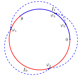
(a) Rotation by the angle $\theta$ equal to the length of the arc $I_{1}$

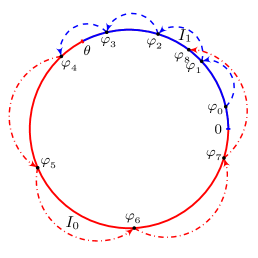
(b) Double rotation: each of the arcs $I_{0}$ and $I_{1}$ is rotated by its own angle

Figure 3. Regular and double rotation of a circle

One of the most important properties of the Sturmian sequences is the following fact (Fogg, 2002, Lemma 6.1.3):

Lemma 2.

In any (generalized) Sturmian sequence consisting of two characters $\{0,1\}$, exactly one of the symbol sequences (words) $\boldsymbol{00}$ or $\boldsymbol{11}$ does not occur.

Lemma 2 becomes clear if we note that the points $\{\varphi_{n}\}$ satisfying (18) cannot fall twice in succession in the interval $[0,\theta)$ or $[\theta,1)$ which has the smallest length.

For illustration, note that the Sturmian index sequence (17) does not contain the symbol sequence (word) $\boldsymbol{00}$.

5. A Pair of Matrices Similar to Plane Rotations

As mentioned in Section 4, previous studies (Lagarias and Wang, 1995; Bousch and Mairesse, 2002; Blondel et al., 2003; Kozyakin, 2005b, 2007) for matrix sets (15) consisting of nonnegative matrices of a special form have provided some clarity on the structure of index sequences that yield the maximal growth rate of matrix product norms. For this reason, in this section we focus on considering less studied matrix sets, namely sets consisting of matrices that may have negative elements. Our goal is to give an example of matrix sets $\mathscr{A}=\{A_{0},A_{1}\}$ consisting of matrices of dimension ${2\times 2}$, in which the sequences of indices $\{\sigma_{i}\}$ maximizing $\|A_{\sigma_{n}}\cdots A_{\sigma_{1}}A_{\sigma_{0}}x\|$, where $\|\cdot\|$ is a Barabanov norm, are not Sturmian! One of the simplest types of this kind of matrix sets is the set of matrices $\mathscr{A}=\{A_{0},A_{1}\}$, where

$$A_{0}=\left[\begin{array}[]{cr}\cos\theta_{0}&-\sin\theta_{0}\\ \sin\theta_{0}&\cos\theta_{0}\end{array}\right],\quad A_{1}=\left[\begin{array}[]{rr}\cos\theta_{1}&-\lambda\sin\theta_{1}\\ \frac{1}{\lambda}\sin\theta_{1}&\cos\theta_{1}\end{array}\right].$$ (21)

Further considerations in this section are based on computational experiments and have no theoretical basis at this time. In this respect, this section should be considered as a kind of set of questions (with accompanying comments) for further research.

Consider the sets of matrices $\mathscr{A}=\{A_{0},A_{1}\}$ defined by the following parameters:

$$\text{Case 1}:\quad \theta_{0} =0.4, \theta_{1} =0.8, \lambda =0.75,$$

$$\text{Case 2}: \theta_{0} \approx 0.6151,\quad \theta_{1} =0.8,\quad \lambda =0.75,$$

$$\text{Case 3}: \theta_{0} =0.7, \theta_{1} =0.8, \lambda =0.75.$$

In these cases, the software tools described in Section 6 allowed not only to visualize approximately the shape of the unit sphere of the Barabanov norm, but also to show examples of iterations $x_{n+1}=A_{\sigma_{n}}x_{n}$ where the maximum growth rate of the Barabanov norm of $\|x_{n}\|$ is reached. It also approximately finds the angular function $\tilde{\varPhi}(\varphi)$ (see (14)) of the matrix set $\mathscr{A}$, whose iterations allow the computation of the angular coordinates $\tilde{\varphi}_{n}$ of the corresponding vectors $x_{n}$, without computing their norms! The results of the corresponding numerical simulations are shown in Figs. 4, 5 and 6. Since the meaning of the notation in these figures repeats verbatim the explanations made for Figs. 1(a), 1(b) and 1(c), we do not present them here.

As can be seen in Figs. 4(a), 5(a), and 6(a), in all three cases the set ${X_{0}\cap X_{1}}$ (see definitions in (10), (11)) turns out to be the union of two straight lines passing through the origin (dash-dotted lines). In this context, the following question arises.

Question 1.

For the case of a pair of nonnegative matrices (15), the statement that the part of the set $X_{0}\cap X_{1}$ passing through the first and third quadrants is a straight line is strictly justified in (Kozyakin, 2005b, 2007). We are not aware of such a proof for the sets of matrices (21) considered in this section. The question arises: Is the set $\boldsymbol{X_{0}\cap X_{1}}$ in this case always the union of two straight lines? And why only of two?∎

From Figs. 4(b), 5(b), and 6(b) it is evident (and it was calculated with the program barnorm_rot.py described in Section 6) that the index sequences of the trajectories with the maximum growth rate in the Barabanov norm, for Cases 1–3, are as follows:

$$\{\sigma_{n}\} =10000110000110000110001100001100001100001100001100\ldots\,,$$

$$\{\sigma_{n}\} =10001100110001100110001100110001100110001100110001\ldots\,,$$

$$\{\sigma_{n}\} =10011001100110001100110011001100110011001100011001\ldots\,.$$

Calculations with the program barnorm_rot.py have shown that in sequences $\{\sigma_{n}\}$ of length 10000 the symbols $\boldsymbol{0}$, $\boldsymbol{1}$, $\boldsymbol{00}$, $\boldsymbol{01}$, $\boldsymbol{10}$ and $\boldsymbol{11}$ occur with the following frequencies:

Symbols	$\boldsymbol{0}$	$\boldsymbol{1}$	$\boldsymbol{00}$	$\boldsymbol{01}$	$\boldsymbol{10}$	$\boldsymbol{11}$
Frequencies (Case 1)	0.655	0.345	0.483	0.172	0.172	0.172
Frequencies (Case 2)	0.555	0.445	0.333	0.222	0.222	0.222
Frequencies (Case 3)	0.517	0.483	0.276	0.241	0.241	0.241

From this, according to Lemma 2, the following fundamentally important conclusion follows.

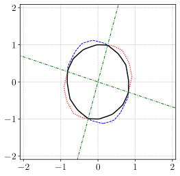
(a) A Barabanov norm

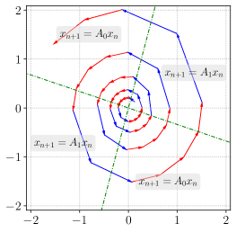
(b) A maximum growth rate trajectory

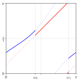
(c) The function $\tilde{\varPhi}(\varphi)$ does not preserve orientation and has two discontinuity points

Figure 4. A Barabanov norm and the angular function: Case 1

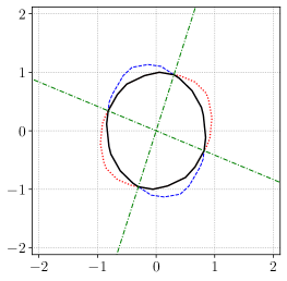
(a) A Barabanov norm

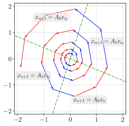
(b) A maximum growth rate trajectory

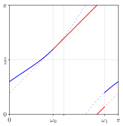
(c) The function $\tilde{\varPhi}(\varphi)$ preserves orientation and has one discontinuity point

Figure 5. A Barabanov norm and the angular function: Case 2

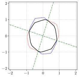
(a) A Barabanov norm

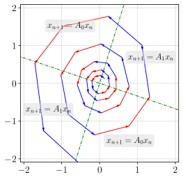
(b) A maximum growth rate trajectory

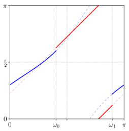
(c) The function $\tilde{\varPhi}(\varphi)$ preserves orientation and has two discontinuity points

Figure 6. A Barabanov norm and the angular function: Case 3

Main Claim.

In the cases of pairs of matrices (21), similar to plane rotations, the index sequences of trajectories with the maximal growth rate in the Barabanov norm are not (generalized) Sturmian.

Let us turn to a more detailed analysis of the obtained results of numerical simulation.

Case 1.

As can be seen from Fig. 4(c), in Case 1 the angular function $\tilde{\varPhi}(\varphi)$, considered as a mapping of the circle into itself, does not preserve orientation. In particular, this situation resembles the behavior of the so-called double rotations (Suzuki et al., 2005; Clack, 2013; Artigiani et al., 2021; Kryzhevich, 2020), defined by the equation

$$f_{\theta_{1},\theta_{2},\theta}(\varphi)=\begin{cases}\varphi+\theta_{1}\bmod 1&\text{for\leavevmode\nobreak\ }x\in[0,\theta),\\ \varphi+\theta_{2}\bmod 1&\text{for\leavevmode\nobreak\ }x\in[\theta,1),\end{cases}$$ (22)

where $(\theta_{1},\theta_{2},\theta)\in[0,1)\times[0,1)\times[0,1)$ are some parameters (see the example in Fig. 3(b)).

The mappings $\tilde{\varPhi}(\varphi)$ and $f_{\theta_{1},\theta_{2},\theta}(\varphi)$ are related by the fact that both are not continuous and do not preserve orientation on a circle but their action is determined by some “rotations” on two continuity intervals of the mappings. The difference between the angular function $\tilde{\varPhi}(\varphi)$ from the double rotations of the circle $f_{\theta_{1},\theta_{2},\theta}(\varphi)$ is that for the first of these mappings, the rotation angles are not constant, while in the case of the mapping $f_{\theta_{1},\theta_{2},\theta}(\varphi)$, the rotation angles are constant for each of the intervals $[0,\theta)$ and $[\theta,1)$. Double rotations of the circle are thus somewhat easier to study, and some progress has been made recently in their analysis (Suzuki et al., 2005; Clack, 2013; Artigiani et al., 2021).

Question 2.

Is it possible (by analogy with the case of the angular function $\tilde{\varPhi}(\varphi)$ for the set of nonnegative matrices (15)) for the angular function $\tilde{\varPhi}(\varphi)$, arising in Case 1, select parameters $\theta_{1}$, $\theta_{2}$, $\theta$ such that the corresponding index sequences for the mapping $\tilde{\varPhi}(\varphi)$ would match the index sequences for the mapping $f(\theta_{1},\theta_{2},\theta)(\varphi)$?∎

A positive answer to this question does not seem very likely. As a first step to clarify the situation, it would be possible to compare the frequencies of occurrence of the symbols $\boldsymbol{0}$ and $\boldsymbol{1}$, as well as groups of consecutive identical symbols $\boldsymbol{00\ldots 0}$ and $\boldsymbol{11\ldots 1}$ in index sequences for the mappings $\tilde{\varPhi}(\varphi)$ and $f(\theta_{1},\theta_{2},\theta)(\varphi)$. Perhaps a negative answer to Question 2 could have been obtained already at this stage.

Question 3.

Again by analogy with the case of the angular function $\tilde{\varPhi}(\varphi)$ for the set of matrices (15): For the angular function $\tilde{\varPhi}(\varphi)$ occurring in Case 1, are there limit frequencies for the occurrence of the symbols $\boldsymbol{0}$ and $\boldsymbol{1}$ in index sequences $\{\sigma_{n}\}$? If the answer is yes, do these frequencies depend on a particular index sequence or not (as in the case of the angular function $\tilde{\varPhi}(\varphi)$ for the matrix set (15))?∎

Question 4.

If Question 3 is answered in the affirmative, then are the limiting frequencies of occurrence of the symbols $\boldsymbol{0}$ and $\boldsymbol{1}$ in the index sequences $\{\sigma_{n}\}$ for the angular function $\tilde{\varPhi}(\varphi)$ dependent on a particular index sequence or not (as in the case of the angular function $\tilde{\varPhi}(\varphi)$ for a set of matrices (15))?∎

In answering Question 4, it might be useful to refer to the theory of circle mappings (Misiurewicz, 1986; Alsedà and Mañosas, 1990, 1996; Alsedà and Moreno, 2000; Misiurewicz, 2007), both continuous and discontinuous, which are not orientation-preserving. Unfortunately, the lack of the orientation preserving property makes the analysis of the mappings of the circle much more difficult. Instead of characterizing the “mean rotation angle” in such mappings by the so-called “rotation number” (a standard tool in the theory of orientation-preserving circle mappings), the concept of a “rotation interval” emerges in non-orientation-preserving circle mappings (Misiurewicz, 1986; Alsedà and Mañosas, 1990; Alsedà and Moreno, 2000; Misiurewicz, 2007). The latter fact may be crucial in answering the question whether the frequency of occurrence of symbols in an index sequence depends on that sequence. Note, however, that in our numerical experiments the dependence of the frequency characteristics on the trajectory was not observed.

Cases 2 and 3.

In these cases the angular function $\tilde{\varPhi}(\varphi)$, considered as a mapping of the circle into itself, preserves orientation. In Case 2 it has one discontinuity point and in Case 3 two, see Figs. 5(c) and 6(c). Therefore (Kozyakin, 2005a, b, 2007), for the mapping $\tilde{\varPhi}(\varphi)$ in these cases, the so-called rotation number $\varkappa(\tilde{\varPhi})$ is defined, which characterizes the “mean rotation angle” performed by this mapping.

In the case where $\tilde{\varPhi}(\varphi)$ is an angular function (12) generated by the pair of nonnegative matrices (15), the rotation number $\varkappa(\tilde{\varPhi})$ coincides with the frequency of hitting the trajectory elements

$$x_{n+1}=A_{\sigma_{n}}x_{n},\qquad n=0,1,\ldots\leavevmode\nobreak\ ,$$

into the set $X_{0}$, and hence with the frequency of occurrence of the symbol $\boldsymbol{0}$ in the corresponding index sequence.

Question 5.

In Cases 2 and 3, as mentioned above, a rotation number is also defined for the mapping $\tilde{\varPhi}(\varphi)$. However, whether this implies the existence of limiting frequencies for the occurrence of the symbols $\boldsymbol{0}$ and $\boldsymbol{1}$ in the index sequences $\{\sigma_{n}\}$ for the angular function $\tilde{\varPhi}(\varphi)$ remains unclear!∎

The behavior of the mapping $\tilde{\varPhi}(\varphi)$, considered as a mapping of a circle, resembles the behavior of the mapping of a circle (18) in Cases 2 and 3:

$$\varphi_{n+1}=\varphi_{n}+\theta\bmod 1,$$ (23)

with the difference that this time the index sequence $\{\sigma_{n}\}$ is not calculated using formula (19), but as follows:

$$\sigma_{n}=\begin{cases}0,&\text{if\leavevmode\nobreak\ }\varphi_{n}\in I_{0}:=[\theta_{0},1),\\ 1,&\text{if\leavevmode\nobreak\ }\varphi_{n}\in I_{1}:=[0,\theta_{0}),\end{cases}$$ (24)

where the length of the interval $I_{1}$ is generally different from the angle of rotation: $\theta_{0}\neq\theta$. As shown in (Berstel and Vuillon, 2002), the behavior of the index sequence (24) can be expressed in terms of a pair of Sturmian sequences generated by rotation through angle $\theta$, but in a rather complex way.

A question similar to that of Question 2 may be asked here.

Question 6.

For the angular function $\tilde{\varPhi}(\varphi)$ occurring in Cases 2 and 3, is it possible to choose the parameters $\theta_{0}$ and $\theta$ such that the corresponding index sequences for $\tilde{\varPhi}(\varphi)$ coincide with the index sequences (24) for the rotation mapping (23)?∎

As in the case of Question 2, a positive answer to this question does not seem very likely. Here, as a first step to clarify the situation, one might compare the frequencies of occurrence of the symbols $\boldsymbol{0}$ and $\boldsymbol{1}$ as well as groups of consecutive identical symbols $\boldsymbol{00\ldots 0}$ and $\boldsymbol{11\ldots 1}$ in index sequences for the mappings $\tilde{\varPhi}(\varphi)$ and (23)–(24). Note, however, that in this case (unlike the situation described in the discussion of Question 4) the computation of the frequency characteristics of the index sequences (24) can be performed theoretically, which is possible may simplify the research.

6. Methods and Tools for Numerical Modeling

In this work, an approximate construction of Barabanov norms of matrix sets (and visualization of their unit spheres as well as the trajectories with the maximum growth rate in the Barabanov norm) was performed using the programs barnorm_sturm.py and barnorm_rot.py, which are available for download from the website https://github.com/kozyakin/barnorm. These programs use a small modification of the max-relaxation algorithm for the iterative construction of Barabanov norms, which can be found in (Kozyakin, 2010a, 2011). The modification compared to the software implementation of the corresponding algorithms described in (Kozyakin, 2010b) was that convex centrally symmetric polygons were chosen as unit spheres of norms approximating the Barabanov norm. The advantage of this approach over the approach of (Kozyakin, 2010b) is that when linear transformations are applied, the unit spheres of the norms $\|A_{0}x\|$ and $\|A_{1}x\|$ are again convex centrally symmetric polygons. Using the library shapely of the language Python, this allows the iterative computation of the norm $\max\{\|A_{0}x\|,\|A_{1}x\|\}$ without loss of precision for each iteration.

The programs barnorm_sturm.py and barnorm_rot.py differ from each other only in the specification of the matrices $A_{0}$ and $A_{1}$ and in the amount of graphical data displayed. Both programs are implemented in the Python programming language of versions 3.8–3.10 of the Miniconda3 (Anaconda3) distribution.

For the convenience of the reader, a listing of the program barnorm_rot.py is provided in Appendix A.

7. Conclusion

The paper presents the results of a numerical simulation of the fastest growing (in the Barabanov norm) trajectories generated by sets of ${2\times 2}$ matrices. The results obtained indicate that in certain situations the maximum growth rate can be achieved on trajectories with non-Sturmian sequences of indices, which makes these situations fundamentally different from most theoretical studies carried out so far in the theory of joint/generalized spectral radius.

Section 5 presents the results of the numerical simulations performed in this paper and formulates a number of open questions. In particular, it would be interesting to compare the complexity functions $p(n,\boldsymbol{\sigma})$ of the index sequences $\boldsymbol{\sigma}=\{\sigma_{n}\}$ of the mappings $\tilde{\varPhi}(\varphi)$ with the complexity functions of the index sequences of the “test” circle mappings (22) and (23)–(24). This question seems all the more interesting because, unlike Sturmian sequences for which the growth rate of the function $p(n,\boldsymbol{\sigma})$ is linear (see (20)), for sequences generated by the double rotation mappings (23)–(24), the growth rate of the complexity function can be superlinear: $p(n,\boldsymbol{\sigma})\sim n^{\gamma}$, where $\gamma>1$ (Clack, 2013). An example of such a growth rate of the norms of matrix products is described in (Hare et al., 2013).

Since the bulk of the results presented above are numerical in nature, this paper should not be considered a full-fledged theoretical study but rather a plan for further research on the subject.

Appendix A Program for Calculating the Barabanov Norm

The code below is written in the Python programming language versions 3.8–3.10 of the Miniconda3 (Anaconda3) distribution. This and some other related scripts for calculating the Barabanov norm can be downloaded from the website https://github.com/kozyakin/barnorm.

⬇

1# -*- coding: utf-8 -*-

2"""Barabanov norms for rotation matrices.

3

4Created on Sat Sep 21 12:37:46 2019.

5Last updated on Wed Apr 27 17:07:05 2022 +0300

6

7@author: Victor Kozyakin

8"""

9import time

10import math

11from matplotlib import pyplot

12from matplotlib.ticker import MultipleLocator

13import numpy as np

14import shapely

15from shapely.geometry import LineString

16from shapely.geometry import MultiPoint

17

18

19def polygonal_norm(_x, _y, _h):

20 """Calculate the norm specified by a polygonal unit ball.

21

22 Args:

23 _x (real): x-coordinate of vector

24 _y (real): y-coordinate of vector

25 _h (MultiPoint): polygonal norm unit ball

26

27 Returns:

28 real: vector’s norm

29 """

30 _hb = _h.bounds

31 _scale = 0.5 * math.sqrt(((_hb[2] - _hb[0])**2 + (_hb[3] - _hb[1])**2) /

32 (_x**2 + _y**2))

33 _ll = LineString([(0, 0), (_scale*_x, _scale*_y)])

34 _h_int = _ll.intersection(_h).coords

35 return math.sqrt((_x**2 + _y**2) / (_h_int[1][0]**2 + _h_int[1][1]**2))

36

37

38def min_max_norms_quotent(_g, _h):

39 """Calculate the min/max of the quotient g-norm/h-norm.

40

41 Args:

42 _g (MultiPoint): polygonal norm unit ball

43 _h (MultiPoint): polygonal norm unit ball

44

45 Returns:

46 2x0-array: mimimum and maximum of g-norm/h-norm

47 """

48 _pg = _g.boundary.coords

49 _dimg = len(_pg) - 1

50 _sg = [1 / polygonal_norm(_pg[i][0], _pg[i][1], _h) for i in range(_dimg)]

51 _ph = _h.boundary.coords

52 _dimh = len(_ph) - 1

53 _sh = [polygonal_norm(_ph[i][0], _ph[i][1], _g) for i in range(_dimh)]

54 _sgh = _sg + _sh

55 return (min(_sgh), max(_sgh))

56

57

58def matrix_angular_coord(_a, _t):

59 """Calculate the angular coordinate of vector Ax given vector x.

60

61 Args:

62 _a (2x2 np.array): input matrix A

63 _t (nx1 np.array): array of input angles of x’s

64

65 Returns:

66 [nx1 np.array]: array of output angles of Ax’s

67 """

68 _cos_t = math.cos(_t)

69 _sin_t = math.sin(_t)

70 _vec_t = np.asarray([_cos_t, _sin_t])

71 _vec_t_transpose = np.transpose(_vec_t)

72 _rot_back = np.asarray([[_cos_t, _sin_t], [-_sin_t, _cos_t]])

73 _vec_a = np.matmul(np.matmul(_rot_back, _a), _vec_t_transpose)

74 return _t + math.atan2(_vec_a[1], _vec_a[0])

75

76

77# Initialization

78

79t_tick = time.time()

80T_BARNORM_COMP = 0.

81

82TOL = 0.0000001

83ANGLE_STEP = 0.01

84LEN_TRAJECTORY = 10000

85NUM_SYMB = 50

86L_BOUND = 0.2

87U_BOUND = 2.2

88

89THETA0 = 0.7 # 0.4 # 0.6151 # one point of discontinuity

90THETA1 = 0.8

91COS_A0 = math.cos(THETA0)

92SIN_A0 = math.sin(THETA0)

93COS_A1 = math.cos(THETA1)

94SIN_A1 = math.sin(THETA1)

95LAMBDA = 0.75

96

97A0 = np.asarray([[COS_A0, -SIN_A0], [SIN_A0, COS_A0]])

98A1 = np.asarray([[COS_A1, -LAMBDA * SIN_A1], [(1 / LAMBDA) * SIN_A1, COS_A1]])

99A0T = np.transpose(A0)

100A1T = np.transpose(A1)

101

102# Computation initialization

103

104if ((np.linalg.det(A0) == 0) or (np.linalg.det(A1) == 0)):

105 raise SystemExit("Set of matrices is degenerate. End of work!")

106

107INV_A0 = np.linalg.inv(A0)

108INV_A1 = np.linalg.inv(A1)

109INV_A0T = np.transpose(INV_A0)

110INV_A1T = np.transpose(INV_A1)

111

112p0 = np.asarray([[1, -1], [1, 1]])

113p0 = np.concatenate((p0, -p0), axis=0)

114p0 = MultiPoint(p0)

115h0 = p0.convex_hull

116

117scale0 = 1 / max(h0.bounds[2], h0.bounds[3])

118h0 = shapely.affinity.scale(h0, xfact=scale0, yfact=scale0)

119

120t_ini = time.time() - t_tick

121

122print(’\n # rho_min rho rho_max Num_edges\n’)

123

124# Computation iterations

125

126NITER = 0.

127while True:

128 t_tick = time.time()

129

130 p0 = np.asarray(MultiPoint(h0.boundary.coords))

131

132 p1 = MultiPoint(np.matmul(p0, INV_A0T))

133 h1 = p1.convex_hull

134

135 p2 = MultiPoint(np.matmul(p0, INV_A1T))

136 h2 = p2.convex_hull

137

138 h12 = h1.intersection(h2)

139 p12 = MultiPoint(h12.boundary.coords)

140

141 rho_minmax = min_max_norms_quotent(h12, h0)

142 rho_max = rho_minmax[1]

143 rho_min = rho_minmax[0]

144

145 rho = (rho_max + rho_min) / 2

146

147 h0 = h0.intersection(shapely.affinity.scale(h12, xfact=rho, yfact=rho))

148

149 T_BARNORM_COMP += (time.time() - t_tick)

150

151 NITER += 1

152 print(f’{NITER:3.0f}.’, f’{rho_min:.6f}’, f’{rho:.6f}’, f’{rho_max:.6f}’,

153 ’ ’, len(h0.boundary.coords) - 1)

154 scale0 = 1 / max(h0.bounds[2], h0.bounds[3])

155 h0 = shapely.affinity.scale(h0, xfact=scale0, yfact=scale0)

156

157 if (rho_max - rho_min) < TOL:

158 break

159

160# Plotting Barabanov norm

161

162t_tick = time.time()

163

164h10 = shapely.affinity.scale(h1, xfact=rho, yfact=rho)

165p10 = np.asarray(MultiPoint(h10.boundary.coords))

166

167h20 = shapely.affinity.scale(h2, xfact=rho, yfact=rho)

168p20 = np.asarray(MultiPoint(h20.boundary.coords))

169

170bb = 1.7 * max(h0.bounds[2], h10.bounds[2], h20.bounds[2],

171 h0.bounds[3], h10.bounds[3], h20.bounds[3])

172

173pyplot.rc(’text’, usetex=True)

174pyplot.rc(’font’, family=’serif’)

175

176# =================================================================

177# Tuning the LaTex preamble (e.g. for international support)

178#

179# pyplot.rcParams[’text.latex.preamble’] = \

180# r’\usepackage[utf8]{inputenc}’ + ’\n’ + \

181# r’\usepackage[russian]{babel}’ + ’\n’ + \

182# r’\usepackage{amsmath}’

183# =================================================================

184

185# Plotting Barabanov’s norm

186

187fig1 = pyplot.figure(1, dpi=108)

188ax1 = fig1.add_subplot(111)

189ax1.set_xlim(-1.1*bb, 1.1*bb)

190ax1.set_ylim(-1.1*bb, 1.1*bb)

191ax1.set_aspect(1)

192ax1.tick_params(labelsize=16)

193ax1.grid(True, linestyle=":")

194ax1.xaxis.set_major_locator(MultipleLocator(1))

195ax1.yaxis.set_major_locator(MultipleLocator(1))

196

197ax1.plot(p10[:, 0], p10[:, 1], ’:’, color=’red’, linewidth=1.25)

198ax1.plot(p20[:, 0], p20[:, 1], ’--’, color=’blue’, linewidth=1)

199ax1.plot(p0[:, 0], p0[:, 1], ’-’, color=’black’)

200

201# Plotting lines of intersection of norms’ unit spheres

202

203pl10 = LineString(p10)

204pl20 = LineString(p20)

205h_int = np.asarray(shapely.affinity.scale(pl10.intersection(pl20),

206 xfact=3, yfact=3))

207arr_switch_N = np.size(h_int[:, 0])

208arr_switch_ang = np.empty(arr_switch_N)

209for i in range(np.size(h_int[:, 0])):

210 arr_switch_ang[i] = math.atan2(h_int[i, 1], h_int[i, 0])

211 if arr_switch_ang[i] < 0:

212 arr_switch_ang[i] = arr_switch_ang[i] + 2. * math.pi

213 if h_int[i, 0] >= 0:

214 ax1.plot([2 * h_int[i, 0], -2 * h_int[i, 0]],

215 [2 * h_int[i, 1], -2 * h_int[i, 1]],

216 dashes=[5, 2, 1, 2], color=’green’, linewidth=1)

217

218t_plot_fig1 = time.time() - t_tick

219pyplot.show()

220

221

222# Plotting an extremal trajectory

223

224t_tick = time.time()

225

226fig2 = pyplot.figure(1, dpi=108)

227ax2 = fig2.add_subplot(111)

228ax2.set_xlim(-1.1*bb, 1.1*bb)

229ax2.set_ylim(-1.1*bb, 1.1*bb)

230ax2.set_aspect(1)

231ax2.tick_params(labelsize=16)

232ax2.grid(True, linestyle=":")

233ax2.xaxis.set_major_locator(MultipleLocator(1))

234ax2.yaxis.set_major_locator(MultipleLocator(1))

235

236# Plotting lines of intersection of norms’ unit spheres

237

238arr_switch_N = np.size(h_int[:, 0])

239arr_switch_ang = np.empty(arr_switch_N)

240for i in range(np.size(h_int[:, 0])):

241 arr_switch_ang[i] = math.atan2(h_int[i, 1], h_int[i, 0])

242 if arr_switch_ang[i] < 0:

243 arr_switch_ang[i] = arr_switch_ang[i] + 2. * math.pi

244 if h_int[i, 0] >= 0:

245 ax2.plot([2 * h_int[i, 0], -2 * h_int[i, 0]],

246 [2 * h_int[i, 1], -2 * h_int[i, 1]],

247 dashes=[5, 2, 1, 2], color=’green’, linewidth=1)

248

249

250# Plotting the trajectory

251

252x = np.asarray([1, 1])

253

254if rho > 1:

255 x = (L_BOUND / polygonal_norm(x[0], x[1], h0)) * x

256else:

257 x = (U_BOUND / polygonal_norm(x[0], x[1], h0)) * x

258

259for i in range(LEN_TRAJECTORY):

260 xprev = x

261 x0 = np.matmul(x, A0T)

262 x1 = np.matmul(x, A1T)

263 if (polygonal_norm(x0[0], x0[1], h0) >

264 polygonal_norm(x1[0], x1[1], h0)):

265 x = x0

266 ax2.arrow(xprev[0], xprev[1], x[0]-xprev[0], x[1]-xprev[1],

267 head_width=0.04, head_length=0.08, linewidth=0.75,

268 color=’red’, length_includes_head=True, zorder=-i)

269 else:

270 x = x1

271 ax2.arrow(xprev[0], xprev[1], x[0]-xprev[0], x[1]-xprev[1],

272 head_width=0.04, head_length=0.08, linewidth=0.75,

273 color=’blue’, length_includes_head=True, zorder=-i)

274 if ((polygonal_norm(x[0], x[1], h0) > U_BOUND) or

275 (polygonal_norm(x[0], x[1], h0) < L_BOUND)):

276 break

277

278arr_switch_ang.sort()

279ISPLIT = 0

280for i in range(np.size(arr_switch_ang)):

281 if arr_switch_ang[i] < math.pi:

282 ISPLIT = i

283

284arr_switch_ang = np.resize(arr_switch_ang, ISPLIT + 1)

285arr_switch_N = np.size(arr_switch_ang)

286arr_switches = np.insert(arr_switch_ang, 0, 0)

287arr_switches = np.append(arr_switches, math.pi)

288omega1 = (arr_switches[1] + arr_switches[2])/2.

289omega2 = omega1 + math.pi/2.

290omega3 = omega2 + math.pi/2.

291omega4 = omega3 + math.pi/2.

292props = dict(boxstyle=’round’, facecolor=’gainsboro’, edgecolor=’none’,

293 alpha=0.5)

294p_label = np.array([math.cos(omega1), math.sin(omega1)])

295

296if (polygonal_norm(p_label[0], p_label[1], h10) >

297 polygonal_norm(p_label[0], p_label[1], h20)):

298 ax2.text(0.9 * bb * math.cos(omega1), 0.9 * bb * math.sin(omega1),

299 r’$x_{n+1}=A_0x_n$’, ha=’center’, va=’center’,

300 fontsize=’x-large’, bbox=props)

301 ax2.text(0.8 * bb * math.cos(omega2), 0.8 * bb * math.sin(omega2),

302 r’$x_{n+1}=A_1x_n$’, ha=’center’, va=’center’,

303 fontsize=’x-large’, bbox=props)

304 ax2.text(0.9 * bb * math.cos(omega3), 0.9 * bb * math.sin(omega3),

305 r’$x_{n+1}=A_0x_n$’, ha=’center’, va=’center’,

306 fontsize=’x-large’, bbox=props)

307 ax2.text(0.8 * bb * math.cos(omega4), 0.8 * bb * math.sin(omega4),

308 r’$x_{n+1}=A_1x_n$’, ha=’center’, va=’center’,

309 fontsize=’x-large’, bbox=props)

310else:

311 ax2.text(0.8 * bb * math.cos(omega1), 0.8 * bb * math.sin(omega1),

312 r’$x_{n+1}=A_1x_n$’, ha=’center’, va=’center’,

313 fontsize=’x-large’, bbox=props)

314 ax2.text(0.9 * bb * math.cos(omega2), 0.9 * bb * math.sin(omega2),

315 r’$x_{n+1}=A_0x_n$’, ha=’center’, va=’center’,

316 fontsize=’x-large’, bbox=props)

317 ax2.text(0.8 * bb * math.cos(omega3), 0.8 * bb * math.sin(omega3),

318 r’$x_{n+1}=A_1x_n$’, ha=’center’, va=’center’,

319 fontsize=’x-large’, bbox=props)

320 ax2.text(0.9 * bb * math.cos(omega4), 0.9 * bb * math.sin(omega4),

321 r’$x_{n+1}=A_0x_n$’, ha=’center’, va=’center’,

322 fontsize=’x-large’, bbox=props)

323

324t_plot_fig2 = time.time() - t_tick

325pyplot.show()

326

327# Plotting the angular functions

328

329t_tick = time.time()

330

331fig3 = pyplot.figure(2, dpi=108)

332ax3 = fig3.add_subplot(111)

333ax3.set_xlim(0., math.pi)

334ax3.set_ylim(0., math.pi)

335ax3.set_aspect(1)

336ax3.tick_params(labelsize=16)

337

338t = np.arange(0., math.pi, ANGLE_STEP)

339angle_arr_A0 = np.empty(len(t))

340angle_arr_A1 = np.empty(len(t))

341for i, item in enumerate(t):

342 angle_arr_A0[i] = matrix_angular_coord(A0, item)

343 angle_arr_A1[i] = matrix_angular_coord(A1, item)

344

345ax3.plot(t, angle_arr_A0, linestyle=(0, (30, 30)), color=’red’,

346 linewidth=0.15)

347ax3.plot(t, angle_arr_A0 + math.pi, linestyle=(0, (30, 30)), color=’red’,

348 linewidth=0.15)

349ax3.plot(t, angle_arr_A0 - math.pi, linestyle=(0, (30, 30)), color=’red’,

350 linewidth=0.15)

351ax3.plot(t, angle_arr_A1, linestyle=(0, (30, 30)), color=’blue’,

352 linewidth=0.15)

353ax3.plot(t, angle_arr_A1 + math.pi, linestyle=(0, (30, 30)), color=’blue’,

354 linewidth=0.15)

355ax3.plot(t, angle_arr_A1 - math.pi, linestyle=(0, (30, 30)), color=’blue’,

356 linewidth=0.15)

357

358# Plotting the angular function delivering

359# the maximal growth rate of iterations

360

361for j in range(arr_switch_N + 1):

362 t = np.arange(arr_switches[j], arr_switches[j + 1], ANGLE_STEP)

363 angle_arr_A0 = np.empty(len(t))

364 angle_arr_A1 = np.empty(len(t))

365 for i, item in enumerate(t):

366 angle_arr_A0[i] = matrix_angular_coord(A0, item)

367 angle_arr_A1[i] = matrix_angular_coord(A1, item)

368 omega = (arr_switches[j] + arr_switches[j + 1]) / 2.

369 x = np.asarray([math.cos(omega), math.sin(omega)])

370 x0 = np.matmul(x, A0T)

371 x1 = np.matmul(x, A1T)

372 if (polygonal_norm(x0[0], x0[1], h0) <

373 polygonal_norm(x1[0], x1[1], h0)):

374 ax3.plot(t, angle_arr_A1, ’b’, linewidth=1.5)

375 ax3.plot(t, angle_arr_A1 + math.pi, ’b’, linewidth=1.5)

376 ax3.plot(t, angle_arr_A1 - math.pi, ’b’, linewidth=1.5)

377 else:

378 ax3.plot(t, angle_arr_A0, ’r’, linewidth=1.5)

379 ax3.plot(t, angle_arr_A0 + math.pi, ’r’, linewidth=1.5)

380 ax3.plot(t, angle_arr_A0 - math.pi, ’r’, linewidth=1.5)

381

382# Putting Pi-ticks on axes

383

384xtick_pos = [0, arr_switches[1], 0.5 * np.pi, arr_switches[2], np.pi]

385xlabels = [r’0’, r’$\omega_0$’, ’’, r’$\omega_1$’, r’$\pi$’]

386ytick_pos = [0, 0.5 * np.pi, np.pi]

387ylabels = [r’0’, r’$\frac{\pi}{2}$’, r’$\pi$’]

388

389pyplot.xticks(xtick_pos, xlabels)

390pyplot.yticks(ytick_pos, ylabels)

391pyplot.grid(linestyle=":")

392

393t_plot_fig3 = time.time() - t_tick

394pyplot.show()

395

396# Calculating index sequence

397

398t_tick = time.time()

399

400F0 = 0.

401F1 = 0.

402F00 = 0.

403F01 = 0.

404F10 = 0.

405F11 = 0.

406x = np.asarray([1, 1])

407index_seq = []

408

409for i in range(LEN_TRAJECTORY):

410 x = x / polygonal_norm(x[0], x[1], h0)

411 x0 = np.matmul(x, A0T)

412 x1 = np.matmul(x, A1T)

413 if (polygonal_norm(x0[0], x0[1], h0) >

414 polygonal_norm(x1[0], x1[1], h0)):

415 x = x0

416 index_seq.append(’0’)

417 F0 += 1

418 else:

419 x = x1

420 index_seq.append(’1’)

421 F1 += 1

422 if i > 0:

423 if ((index_seq[i-1] == ’0’) and (index_seq[i] == ’0’)):

424 F00 += 1

425 if ((index_seq[i-1] == ’0’) and (index_seq[i] == ’1’)):

426 F01 += 1

427 if ((index_seq[i-1] == ’1’) and (index_seq[i] == ’0’)):

428 F10 += 1

429 if ((index_seq[i-1] == ’1’) and (index_seq[i] == ’1’)):

430 F11 += 1

431

432print(’\nExtremal index sequence: ’, end=’’)

433for i in range(NUM_SYMB):

434 print(index_seq[i], end=’’)

435

436print(’\n\nFrequences of symbols 0, 1, 00, 01 etc. in the index sequence:’,

437 ’\n\nSymbols: 0 1 00 01 10 11’)

438

439print(’Frequences: ’,

440 f’ {round(F0/LEN_TRAJECTORY, 3):.3f}’,

441 f’ {round(F1/LEN_TRAJECTORY, 3):.3f}’,

442 f’ {round(F00/(LEN_TRAJECTORY-1), 3):.3f}’,

443 f’ {round(F01/(LEN_TRAJECTORY-1), 3):.3f}’,

444 f’ {round(F10/(LEN_TRAJECTORY-1), 3):.3f}’,

445 f’ {round(F11/(LEN_TRAJECTORY-1), 3):.3f}’)

446

447t_index_seq = time.time() - t_tick

448

449# Saving plots to pdf-files

450

451"""

452fig1.savefig(f’bnorm-{THETA0:.2f}-{THETA1:.2f}-{LAMBDA:.2f}.pdf’,

453 bbox_inches=’tight’)

454fig2.savefig(f’etraj-{THETA0:.2f}-{THETA1:.2f}-{LAMBDA:.2f}.pdf’,

455 bbox_inches=’tight’)

456fig3.savefig(f’sfunc-{THETA0:.2f}-{THETA1:.2f}-{LAMBDA:.2f}.pdf’,

457 bbox_inches=’tight’)

458"""

459

460# Computation timing

461

462t_compute = T_BARNORM_COMP + t_index_seq

463t_total = (t_ini + t_plot_fig3 + t_plot_fig2 + t_plot_fig1 + t_compute)

464t_plot = (t_plot_fig1 + t_plot_fig2 + t_plot_fig3)

465

466print(’\nInitialization: ’, f’{round(t_ini, 6):6.2f} sec.’)

467print(’Computations: ’, f’{round(t_compute, 6):6.2f} sec.’)

468print(’Plotting: ’, f’{round(t_plot, 6):6.2f} sec.’)

469print(’Total: ’, f’{round(t_total, 6):6.2f} sec.’)

Listing 1: Python code barnorm_rot.py for computing the Barabanov norm of a pair of matrices and the angular function of the iterations at which the joint spectral radius is reached

References

- (1)
- Alsedà and Mañosas (1990) Alsedà, L., Mañosas, F., 1990. Kneading theory and rotation intervals for a class of circle maps of degree one. Nonlinearity 3, 413–452. URL: https://iopscience.iop.org/article/10.1088/0951-7715/3/2/008.
- Alsedà and Mañosas (1996) Alsedà, L., Mañosas, F., 1996. Kneading theory for a family of circle maps with one discontinuity. Acta Math. Univ. Comenian. (N.S.) 65, 11–22.
- Alsedà and Moreno (2000) Alsedà, L., Moreno, J.M., 2000. On the rotation sets for non-continuous circle maps. Acta Math. Univ. Comenian. (N.S.) 69, 115–125.
- Artigiani et al. (2021) Artigiani, M., Fougeron, C., Hubert, P., Skripchenko, A., 2021. A note on double rotations of infinite type. ArXiv.org e-Print archive. URL: https://arxiv.org/abs/2102.11803, doi:10.48550/arXiv.2102.11803, arXiv:2102.11803.
- Barabanov (1988a) Barabanov, N.E., 1988a. Lyapunov indicator of discrete inclusions. I. Autom. Remote Control 49, 152–157.
- Barabanov (1988b) Barabanov, N.E., 1988b. The Lyapunov indicator of discrete inclusions. II. Autom. Remote Control 49, 283–287.
- Barabanov (1988c) Barabanov, N.E., 1988c. The Lyapunov indicator of discrete inclusions. III. Autom. Remote Control 49, 558–565.
- Berger and Wang (1992) Berger, M.A., Wang, Y., 1992. Bounded semigroups of matrices. Linear Algebra Appl. 166, 21–27. URL: https://www.sciencedirect.com/science/article/pii/002437959290267E, doi:10.1016/0024-3795(92)90267-E.
- Berstel and Karhumäki (2003) Berstel, J., Karhumäki, J., 2003. Combinatorics on words—a tutorial. Bull. Eur. Assoc. Theor. Comput. Sci. EATCS 79, 178–228. URL: https://www.worldscientific.com/doi/abs/10.1142/9789812562494_0059, doi:10.1142/9789812562494_0059.
- Berstel and Vuillon (2002) Berstel, J., Vuillon, L., 2002. Coding rotations on intervals. Theoret. Comput. Sci. 281, 99–107. URL: https://www.sciencedirect.com/science/article/pii/S0304397502000099, doi:10.1016/S0304-3975(02)00009-9, arXiv:math/0106217.
- Bertsekas and Tsitsiklis (1989) Bertsekas, D.P., Tsitsiklis, J.N., 1989. Parallel and Distributed Computation. Numerical Methods. Prentice Hall, Englewood Cliffs. NJ.
- Blondel and Canterini (2003) Blondel, V.D., Canterini, V., 2003. Undecidable problems for probabilistic automata of fixed dimension. Theory Comput. Syst. 36, 231–245. URL: https://link.springer.com/article/10.1007/s00224-003-1061-2, doi:10.1007/s00224-003-1061-2.
- Blondel et al. (2006) Blondel, V.D., Jungers, R., Protasov, V., 2006. On the complexity of computing the capacity of codes that avoid forbidden difference patterns. IEEE Trans. Inform. Theory 52, 5122–5127. URL: https://ieeexplore.ieee.org/document/1715550, doi:10.1109/TIT.2006.883615, arXiv:cs/0601036.
- Blondel et al. (2003) Blondel, V.D., Theys, J., Vladimirov, A.A., 2003. An elementary counterexample to the finiteness conjecture. SIAM J. Matrix Anal. Appl. 24, 963–970 (electronic). URL: https://epubs.siam.org/sima/resource/1/sjmael/v24/i4/p963_s1, doi:10.1137/S0895479801397846.
- Blondel and Tsitsiklis (2000) Blondel, V.D., Tsitsiklis, J.N., 2000. A survey of computational complexity results in systems and control. Automatica J. IFAC 36, 1249–1274. URL: https://www.sciencedirect.com/science/article/pii/S0005109800000509, doi:10.1016/S0005-1098(00)00050-9.
- Bousch and Mairesse (2002) Bousch, T., Mairesse, J., 2002. Asymptotic height optimization for topical IFS, Tetris heaps, and the finiteness conjecture. J. Amer. Math. Soc. 15, 77–111 (electronic). URL: https://www.ams.org/journals/jams/2002-15-01/S0894-0347-01-00378-2/, doi:10.1090/S0894-0347-01-00378-2.
- Brayton and Tong (1979) Brayton, R.K., Tong, C.H., 1979. Stability of dynamical systems: a constructive approach. IEEE Trans. Circuits Syst. 26, 224–234. URL: https://ieeexplore.ieee.org/document/1084637, doi:10.1109/TCS.1979.1084637.
- Chazan and Miranker (1969) Chazan, D., Miranker, W., 1969. Chaotic relaxation. Linear Algebra Appl. 2, 199–222. URL: https://www.sciencedirect.com/science/article/pii/0024379569900287, doi:10.1016/0024-3795(69)90028-7.
- Clack (2013) Clack, G., 2013. Double Rotations. Ph.D. thesis. University of Surrey (United Kingdom). Guildford. URL: https://openresearch.surrey.ac.uk/esploro/outputs/doctoral/Double-Rotations/99511546402346.
- Daubechies and Lagarias (1992) Daubechies, I., Lagarias, J.C., 1992. Sets of matrices all infinite products of which converge. Linear Algebra Appl. 161, 227–263. URL: https://www.sciencedirect.com/science/article/pii/002437959290012Y, doi:10.1016/0024-3795(92)90012-Y.
- Daubechies and Lagarias (2001) Daubechies, I., Lagarias, J.C., 2001. Corrigendum/addendum to: “Sets of matrices all infinite products of which converge” [Linear Algebra Appl. 161 (1992), 227–263; MR1142737 (93f:15006)]. Linear Algebra Appl. 327, 69–83. URL: https://www.sciencedirect.com/science/article/pii/S0024379500003141, doi:10.1016/S0024-3795(00)00314-1.
- Fogg (2002) Fogg, N.P., 2002. Substitutions in dynamics, arithmetics and combinatorics. volume 1794 of Lecture Notes in Mathematics. Springer-Verlag, Berlin. URL: https://link.springer.com/book/10.1007/b13861, doi:10.1007/b13861. edited by V. Berthé, S. Ferenczi, C. Mauduit and A. Siegel.
- Hare et al. (2013) Hare, K.G., Morris, I.D., Sidorov, N., 2013. Extremal sequences of polynomial complexity. Math. Proc. Cambridge Philos. Soc. 155, 191–205. URL: https://dx.doi.org/10.1017/S0305004113000157, doi:10.1017/S0305004113000157, arXiv:1201.6236.
- Heil and Strang (1995) Heil, C., Strang, G., 1995. Continuity of the joint spectral radius: application to wavelets, in: Linear algebra for signal processing (Minneapolis, MN, 1992). Springer, New York. volume 69 of IMA Vol. Math. Appl., pp. 51–61. doi:10.1007/978-1-4612-4228-4_4.
- Horn and Johnson (1985) Horn, R.A., Johnson, C.R., 1985. Matrix analysis. Cambridge University Press, Cambridge. doi:10.1017/CBO9780511810817.
- Jungers (2009) Jungers, R., 2009. The joint spectral radius. volume 385 of Lecture Notes in Control and Information Sciences. Springer-Verlag, Berlin. URL: https://link.springer.com/book/10.1007/978-3-540-95980-9, doi:10.1007/978-3-540-95980-9. Theory and applications.
- Jungers et al. (2008) Jungers, R.M., Protasov, V., Blondel, V.D., 2008. Efficient algorithms for deciding the type of growth of products of integer matrices. Linear Algebra Appl. 428, 2296–2311. URL: https://www.sciencedirect.com/science/article/pii/S0024379507003436, doi:10.1016/j.laa.2007.08.001.
- Kozyakin (2005a) Kozyakin, V., 2005a. A dynamical systems construction of a counterexample to the finiteness conjecture, in: Proceedings of the 44th IEEE Conference on Decision and Control, 2005 and 2005 European Control Conference. CDC-ECC’05., pp. 2338–2343. URL: https://ieeexplore.ieee.org/document/1582511, doi:10.1109/CDC.2005.1582511.
- Kozyakin (2010a) Kozyakin, V., 2010a. Iterative building of Barabanov norms and computation of the joint spectral radius for matrix sets. Discrete Contin. Dyn. Syst. Ser. B 14, 143–158. URL: https://www.aimsciences.org/article/doi/10.3934/dcdsb.2010.14.143, doi:10.3934/dcdsb.2010.14.143, arXiv:0810.2154.
- Kozyakin (2010b) Kozyakin, V., 2010b. Max-Relaxation iteration procedure for building of Barabanov norms: Convergence and examples. ArXiv.org e-Print archive. URL: https://arxiv.org/abs/1002.3251, doi:10.48550/arXiv.1002.3251, arXiv:1002.3251.
- Kozyakin (2011) Kozyakin, V., 2011. A relaxation scheme for computation of the joint spectral radius of matrix sets. J. Differ. Equations Appl. 17, 185–201. URL: https://www.tandfonline.com/doi/abs/10.1080/10236198.2010.549008, doi:10.1080/10236198.2010.549008, arXiv:0810.4230.
- Kozyakin (2013a) Kozyakin, V., 2013a. An annotated bibliography on the convergence of matrix products and the theory of joint/generalized spectral radius. Preprint. Institute for Information Transmission Problems. Moscow. URL: https://kozyakin.github.io/jsrbib/JSRbib.html, doi:10.13140/RG.2.1.4257.5040/1.
- Kozyakin (1990) Kozyakin, V.S., 1990. Algebraic unsolvability of problem of absolute stability of desynchronized systems. Autom. Remote Control 51, 754–759.
- Kozyakin (2003) Kozyakin, V.S., 2003. Indefinability in o-minimal structures of finite sets of matrices whose infinite products converge and are bounded or unbounded. Autom. Remote Control 64, 1386–1400. URL: https://link.springer.com/article/10.1023/A/:1026091717271, doi:10.1023/A:1026091717271.
- Kozyakin (2005b) Kozyakin, V.S., 2005b. Rotation numbers of discontinuous orientation-preserving circle maps revisited. Information Processes 5, 301–335. URL: http://www.jip.ru/2005/283-300.pdf.
- Kozyakin (2007) Kozyakin, V.S., 2007. Structure of extremal trajectories of discrete linear systems and the finiteness conjecture. Autom. Remote Control 68, 174–209. URL: https://link.springer.com/article/10.1134/S0005117906040171, doi:10.1134/S0005117906040171.
- Kozyakin (2013b) Kozyakin, V.S., 2013b. Algebraic unsolvability of problem of absolute stability of desynchronized systems revisited. ArXiv.org e-Print archive. URL: https://arxiv.org/abs/1301.5409, doi:10.48550/arXiv.1301.5409, arXiv:1301.5409.
- Kryzhevich (2020) Kryzhevich, S., 2020. Invariant measures for interval translations and some other piecewise continuous maps. Math. Model. Nat. Phenom. 15, 15. URL: https://www.mmnp-journal.org/articles/mmnp/abs/2020/01/mmnp180201, doi:10.1051/mmnp/2019041.
- Lagarias and Wang (1995) Lagarias, J.C., Wang, Y., 1995. The finiteness conjecture for the generalized spectral radius of a set of matrices. Linear Algebra Appl. 214, 17–42. URL: https://www.sciencedirect.com/science/article/pii/0024379593000522, doi:10.1016/0024-3795(93)00052-2.
- Lothaire (2002) Lothaire, M., 2002. Algebraic combinatorics on words. volume 90 of Encyclopedia of Mathematics and its Applications. Cambridge University Press, Cambridge. URL: https://www.cambridge.org/core/books/algebraic-combinatorics-on-words/F0C477102253C41503EB7D6AE7C0F367, doi:10.1017/CBO9781107326019.
- Maesumi (1998) Maesumi, M., 1998. Calculating joint spectral radius of matrices and Hölder exponent of wavelets, in: Approximation theory IX, Vol. 2 (Nashville, TN, 1998). Vanderbilt Univ. Press, Nashville, TN. Innov. Appl. Math., pp. 205–212.
- Misiurewicz (1986) Misiurewicz, M., 1986. Rotation intervals for a class of maps of the real line into itself. Ergodic Theory Dynam. Systems 6, 117–132. URL: https://dx.doi.org/10.1017/S0143385700003321, doi:10.1017/S0143385700003321.
- Misiurewicz (2007) Misiurewicz, M., 2007. Rotation theory. Scholarpedia 2, 3873. URL: http://www.math.iupui.edu/~mmisiure/rotth.pdf, doi:10.4249/scholarpedia.3873.
- Moision et al. (2001) Moision, B.E., Orlitsky, A., Siegel, P.H., 2001. On codes that avoid specified differences. IEEE Trans. Inform. Theory 47, 433–442. URL: https://ieeexplore.ieee.org/document/904557, doi:10.1109/18.904557.
- Rota and Strang (1960) Rota, G.C., Strang, G., 1960. A note on the joint spectral radius. Koninklijke Nederlandse Akademie van Wetenschappen. Indagationes Mathematicae 22, 379–381. URL: https://www.sciencedirect.com/science/article/pii/S1385725860500461, doi:10.1016/S1385-7258(60)50046-1.
- Shorten et al. (2007) Shorten, R., Wirth, F., Mason, O., Wulff, K., King, C., 2007. Stability criteria for switched and hybrid systems. SIAM Rev. 49, 545–592. URL: https://epubs.siam.org/sirev/resource/1/siread/v49/i4/p545_s1, doi:10.1137/05063516X.
- Suzuki et al. (2005) Suzuki, H., Ito, S., Aihara, K., 2005. Double rotations. Discrete Contin. Dyn. Syst. 13, 515–532. URL: http://www.aimsciences.org/article/doi/10.3934/dcds.2005.13.515, doi:10.3934/dcds.2005.13.515.
- Tsitsiklis and Blondel (1997) Tsitsiklis, J.N., Blondel, V.D., 1997. The Lyapunov exponent and joint spectral radius of pairs of matrices are hard — when not impossible — to compute and to approximate. Math. Control Signals Systems 10, 31–40. URL: https://link.springer.com/article/10.1007/BF01219774, doi:10.1007/BF01219774.
- Wirth (2002) Wirth, F., 2002. The generalized spectral radius and extremal norms. Linear Algebra Appl. 342, 17–40. URL: https://www.sciencedirect.com/science/article/pii/S0024379501004463, doi:10.1016/S0024-3795(01)00446-3.
- Wu and He (2020) Wu, Z., He, Q., 2020. Optimal switching sequence for switched linear systems. SIAM J. Control Optim. 58, 1183–1206. URL: https://epubs.siam.org/doi/10.1137/18M1197928, doi:10.1137/18M1197928.