Deep Measurement Updates for Bayes Filters
Abstract
Measurement update rules for Bayes filters often contain hand-crafted heuristics to compute observation probabilities for high-dimensional sensor data, like images.
In this work, we propose the novel approach Deep Measurement Update (DMU) as a general update rule for a wide range of systems.
DMU has a conditional encoder-decoder neural network structure to process depth images as raw inputs. Even though the network is trained only on synthetic data, the model shows good performance at evaluation time on real-world data.
With our proposed training scheme primed data training, we demonstrate how the DMU models can be trained efficiently to be sensitive to condition variables without having to rely on a stochastic information bottleneck.
We validate the proposed methods in multiple scenarios of increasing complexity, beginning with the pose estimation of a single object to the joint estimation of the pose and the internal state of an articulated system.
Moreover, we provide a benchmark against Articulated Signed Distance Functions(A-SDF) on the RBO dataset as a baseline comparison for articulation state estimation.
Index Terms:
Sensor Fusion; Deep Learning for Visual Perception; Deep Learning MethodsI INTRODUCTION
In computer vision, many research works have focused on the problem of directly inferring state information from sensor measurements [1, 2, 3].
However, only partial observations are available for many real-world robotics applications, and the entire system state cannot be inferred from a single measurement.
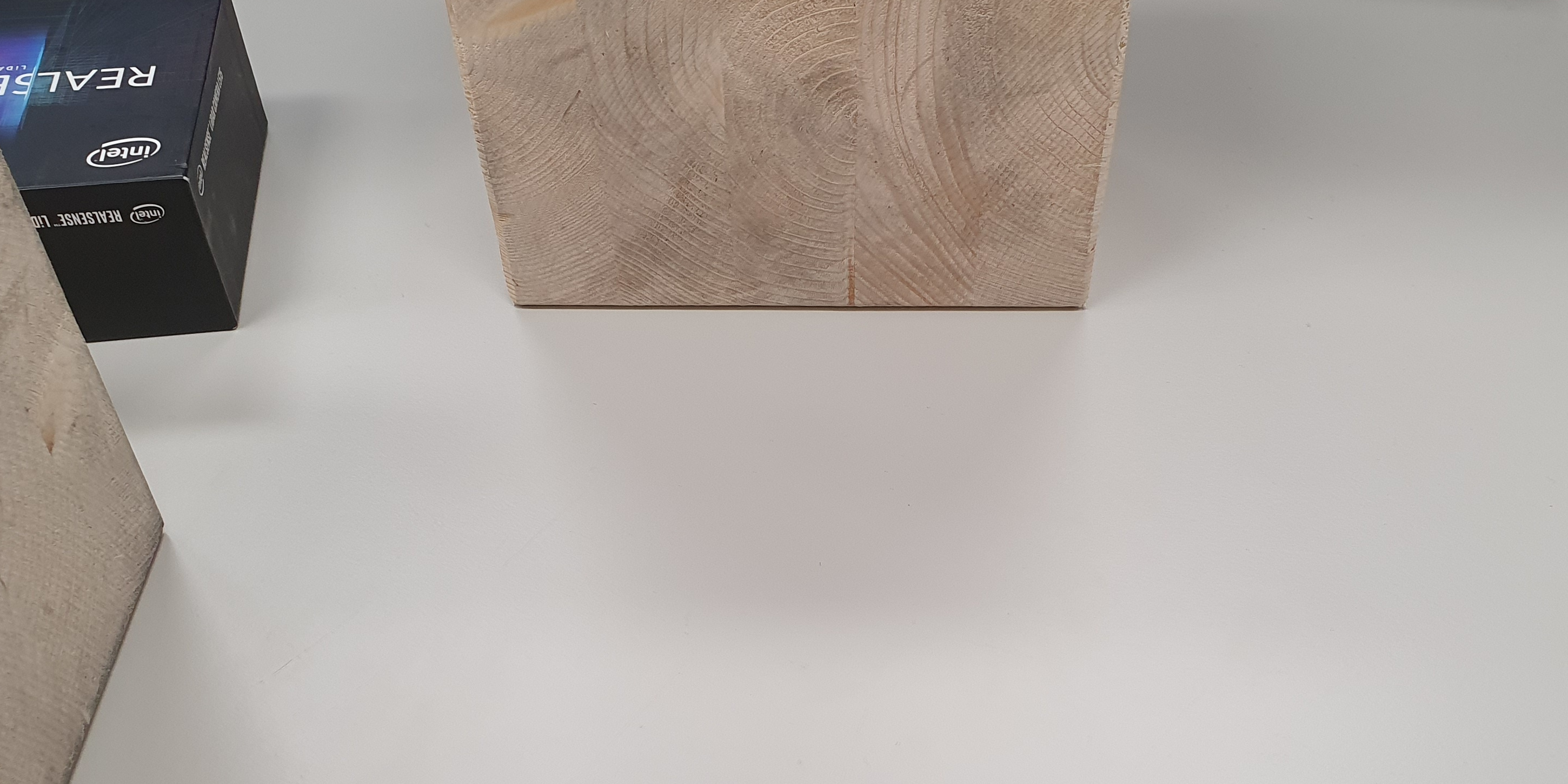
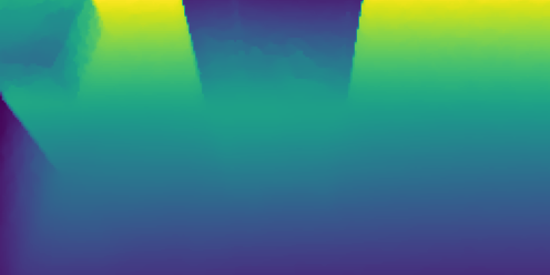
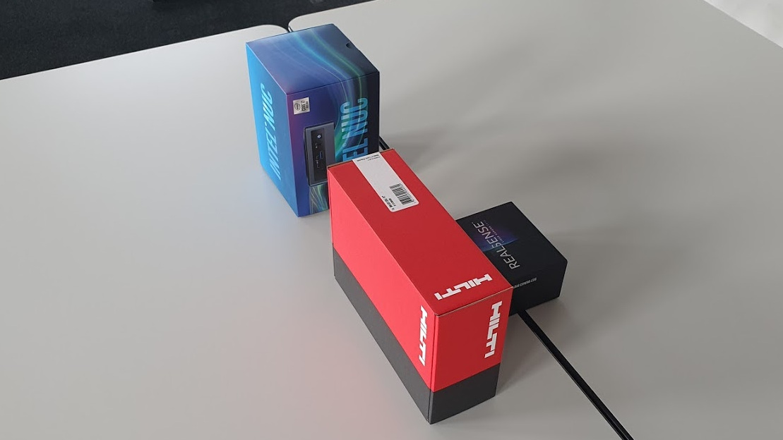
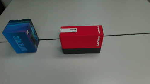
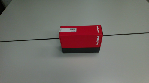
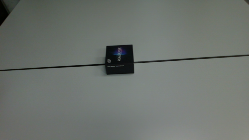
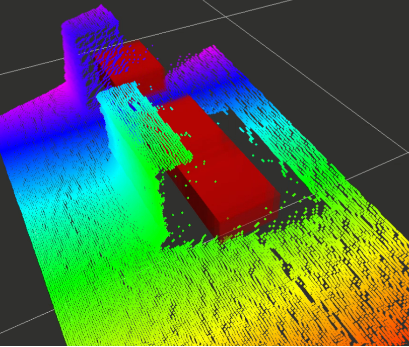
In Fig. 1, an example is presented in which a target object is fully occluded. Free space can however be observed and information on the object pose can be indirectly inferred.
A sequence of measurements and prior knowledge is often needed to estimate the full system state.
Bayes Filters provide a general way to solve this problem [4]. Using the Markov assumption, this framework aims to recursively compute the belief of the state at time given the prior belief and the observation .
In this work, we take a detailed look at how to update the predicted belief from a measurement:
| (1) |
In (1), is a normalizing factor and is the conditional probability density function (CPDF) of a measurement , conditioned on the current system state .
In the following, we drop the superscripts since we do not focus on the time evolution aspect of Bayes filtering.
Finding the CPDF can be viewed as the inverse problem of inferring the state from measurements. In practical robotic applications, this conditional probability is difficult to determine.
Often, hand-crafted sensor processing pipelines are designed and tuned and measurement probabilities are being assigned solely based on heuristics [4, 5].
In this work, we want to use deep learning to find a systematic approach for determining .We propose a conditional auto-encoder (CAE) architecture to learn the probability distribution of possible measurements that can be observed for our system, conditioned on the ground truth system state. Learning the probability distribution associated with high-dimensional training data is addressed by generative models, which include several deep-learning architectures [6, 7, 8, 9, 10, 11].
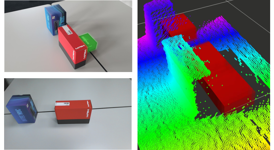
Lower left: The same scene from the point of view of the depth sensor. The target box is occluded.
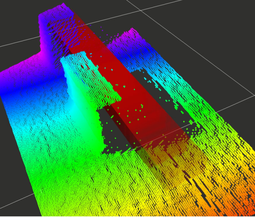
Right: Particle filter estimation of the box pose. A depth image of the scene is displayed as a point cloud. The distribution of 100 particles is visualized with overlaying red semi-transparent boxes. DMU is run on the depth image and assigns a higher observation probability to the particles behind the obstacles than those in visible free space.
Conditional Variational Auto Encoders (CVAEs) [10] offer a general method to perform an approximate inference of the probability of the training data, based on some input observation. They have been shown to be successful in generating output samples that behave according to the underlying probability distribution of the training data. However, numerical evaluation of the marginalized conditional probability requires Monte Carlo sampling on the latent code distribution [10] for each queried system state , making inference slow. Furthermore, balancing the evidence lower bound objective (ELBO) to condition the latent state distribution and the reconstruction loss adds more complexity to the task.
The proposed CAE architecture makes the sampling step superfluous. It allows to efficiently compute and evaluate the measurement probability for integration in the filter update rule.
Learning to extract a state-independent latent code from the input observation is an additional challenge. The difficulty increases when the state dimension is much smaller than the latent code dimension.
For instance, in visual object localization, the state includes the object pose and the latent distribution needs to describe the, possibly highly complex, image background.
In preliminary tests, we found that the trained models relied entirely on the latent code to capture both background and state information. The CAE degenerated to a non-conditional autoencoder.
To overcome this issue, we propose a new training method, named primed data training, which requires the network to synthesize observations with the same background information as the input, but a different conditional state.
Primed data training successfully conditions the network on the state variable. We validate the training scheme on our proposed CAE architecture, although we point out its generality and possible applicability with different conditional models, such as CVAEs or Conditional Normalizing Flows [12].
I-A Related Work
Methods for single-shot object pose detection are well established in the computer-vision and robotics literature [3, 13]. Those works are conceptually very different from ours since they solely focus on the specific problem of pose estimation and cannot easily be applied to a broader class of state estimation problems.
DeepIM [14] uses a render-and-compare approach to refine 6D pose estimates. It uses synthetically rendered images that a learned model compares to the input image. In our work, we also render images and compare them to the input image. However, our rendering is done by a decoder network that can process both the state provided explicitly and information extracted from the input image by the encoder network.
One of the demo cases we present in this paper is articulation state estimation. We benchmark against Articulated Signed Distance Functions (A-SDF) [15], a method that shows good performance on the RBO dataset [16]. Unlike our work, A-SDF requires pre-processing with segmentation masks and is prohibitively slow for real-time applications.
In recent years, Bayes Filtering has regained the attention of researchers from the deep learning community.
Methods like Deep Kalman Filter learn variational models from sequence data [17, 18, 19]. In contrast to our work, their learned system states are latent variables that cannot be interpreted directly.
Particles filter networks [20] learn an observation model to compute the weights required for resampling in a particle filter. In contrast to our work, they do not use a generative model to predict a measurement given a particle state but directly infer weights.
This requires them to train the system end-to-end on sequence data since no ground truth weights are available.
Some works use learned models to extract state information from input images and process the information with Bayes filters [21]. This approach is different from ours since we do not require problem-specific heuristics to perform measurement updates.
I-B Contributions
The contribution of this paper is twofold:
A new approach to learn measurement update rules for Bayes filters is presented.
Second, we propose a novel training scheme, primed data training, which enforces decoder sensitivity to condition variables without introducing a stochastic information bottleneck usually found in CVAEs.
The learned models, which are trained only on synthetic data, are validated in real-world experiments.
II METHODS
II-A Deep Measurement Update
Let be the model of a system. is the state the system is currently in. Such a model is a simplified abstraction of the real world in which only those parts of the world are described that are relevant for a particular task. The state vector may contain heterogeneous elements such as position vectors, orientation quaternions, or categorical variables.
We call the unmodeled part of the reality and the corresponding unmodeled state. For instance, in a perception problem for robotic manipulation, could represent the pose of the object that needs to be grasped by a robot. In the same scenario, would correspond to the state of the background and surrounding objects. A measurement usually does not only depend on the modeled system state but also on the unmodeled state . We suppose that there exists a function that uniquely maps and to a measurement .
Suppose the system is in the state and the measurement is observed.
We want to infer for a set of particles by computing the similarity of the corresponding measurements to .
We assume that , given .
Since the measurements do not only depend on the known states but also the unmodeled part of the system, they cannot trivially be rendered with the function since is usually not known.
We propose to use a conditional encoder-decoder network to render a measurement given the state without explicit knowledge of the unmodeled state .
Fig. 2 shows the structure of the proposed method.
An encoder network extracts a latent code from an input measurement . The latent code resembles the unmodeled state . Together with the modeled state vector , the decoder generates the measurement .
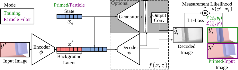
In this work, we call the encoder-decoder combination Conditional Autoencoder (CAE), which is slightly inaccurate nomenclature since the learned network transcodes the tuple to the target .
II-B Primed Data Training
Training the CAE is challenging since the encoder network has to learn how to extract a latent code that only describes the unmodeled state while ignoring the dependencies.
CVAEs achieve this separation between the latent code and the condition variable by imposing structure on the latent code: the encoder network does not directly infer the latent code but the parameters of a normal distribution and . The latent code is then sampled from the distribution . A Kullback-Leibler divergence cost term penalizes deviations of from the standard normal distribution.
This approach is not suitable for our problem. A CVAE only allows for sampling from the distribution of all possible unmodeled states but does not extract the specific instance we need to reconstruct from .
Instead, we achieve the separation by training the networks with primed synthetic data: a synthetic data generator implements the function . z is some parametrization of but typically not identical to the one that the encoder-decoder network learns. We use to generate two measurements: and .
Both measurements are based on different modeled states but share the same unmodeled state. During training, we provide as an input to the encoder and as a condition variable. The training loss is the similarity between the decoder output and the synthetic measurement .
| (2) |
This encourages the encoder network to ignore the influence of on and only focus on the regression of z since this information is necessary to perform well in the task of generating with the decoder.
III Implementation
III-A Network Architecture
Two different Conditional Autoencoder networks have been evaluated.
The basic CAE has an encoder and a decoder network. The encoder network compresses the input image with 6 convolutional layers followed by 3 linear layers all with Relu activations to a 64 dimensional latent vector. The decoder network reconstructs a depth image from the latent vector and the state vector with 6 deconvolutional layers.
The CAE with Generator network shares the basic building blocks with the CAE except that it has an additional generator module consisting of 7 convolutional layers. The generator output is combined with the decoder output in the output conv module with 2 convolutional layers.
The rationale behind the encoder and decoder structure is described in subsection II-A. The generator network supports the decoder in delivering high-quality reconstructions by increasing the emphasis on the modeled state dependency. Conceptually it can be viewed as a part of the decoder implementation.
Convolutional layers extract local features from their inputs or reconstruct pixels from those features in the case of deconvolution. However, they lack a sense of global positioning information in an image. We found that this increases the difficulty of creating good reconstructions. To alleviate that problem, we use Coordinate Convolutional (CoordConv) Layers that take the horizontal and vertical pixel coordinates as additional inputs [22].
The decoder and encoder use kernel size 4 and stride 2; the generator and output networks only employ kernel size 1 convolutions with stride 1.
III-B Training
A data loader has been implemented that generates training data in parallel to the training process. It uses Nvidia’s Issac Sim111https://developer.nvidia.com/isaac-sim to generate batches of depth image pairs with a resolution of along with their corresponding states.
The use of depth images over RGB data is motivated by recent works showing that depth images can transfer from simulation to real applications [23], [24], [25].
Additionally, we generate segmentation masks for the image with problem-specific regions of interest labeled.
samples are generated for each epoch which are reused times in shuffled order. The minibatch size is set to .
As a loss function we use the L1-norm between and .
During experimentation, we noticed an imbalance in the number of pixels affected by the difference between and and the parts of the image that only depend on and are therefore equal between and . To counteract the imbalance, we use the segmentation mask to compute the losses for labeled and unlabeled pixels separately. The total loss is the sum of both labeled and unlabeled loss with mean normalization applied over all pixels in a mini-batch for the separate loss terms. At test time, the segmentation masks are not available, and we compute the loss as described in (2).
The networks are trained on an Nvidia RTX 2080 Super GPU with an Adam optimizer [26] and a learning rate of until convergence.

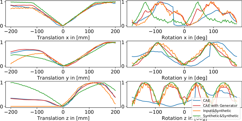
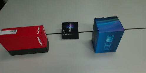
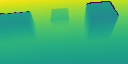
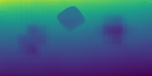
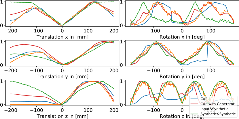
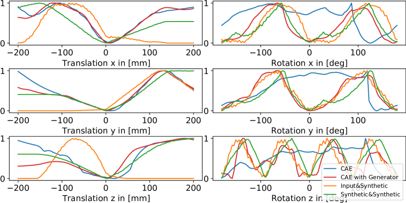


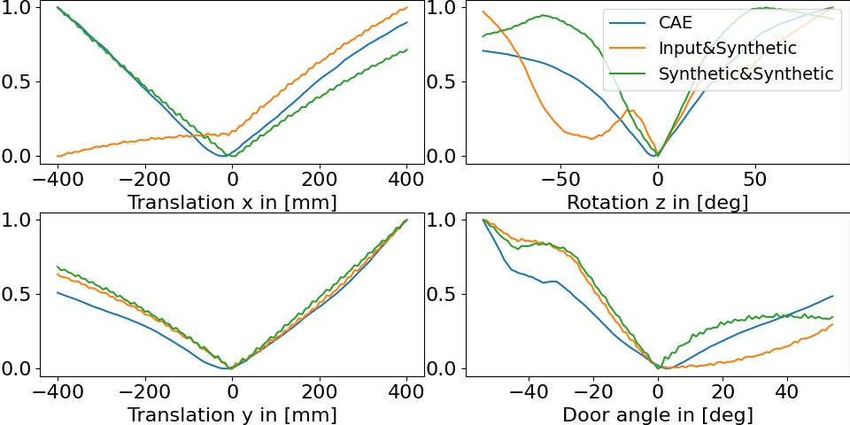
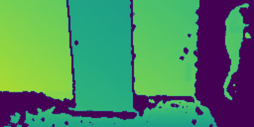
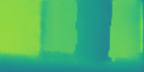
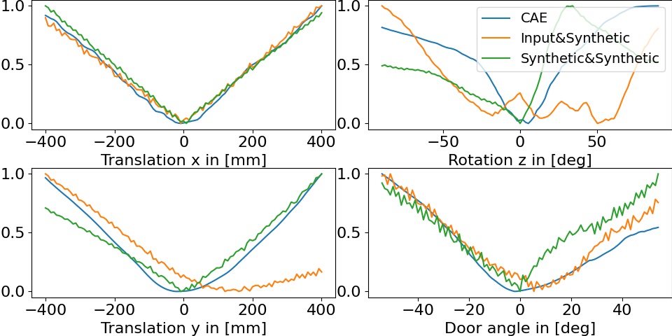
Column 1 gives an overview of the scene. Column 2 shows the recorded depth images. In column 3, reconstructions of the depth images with state vectors deviating from the ground truth are shown. Column 4 shows the loss evaluated as a function of the state for the trained models CAE (blue) and CAE with Generator (red) and the two benchmark quantities Input&Synthetic (orange) and Synthetic&Synthetic (green). For the symmetric pose experiments the state vector is the object pose in camera frame. In the switchboard cabinet experiment, the state vector is the translation of the cabinet, the yaw angle, and the door opening angle.
IV EXPERIMENTS
We present several experimental evaluations of the proposed method. In Sec. IV-A, we demonstrate how the method can be used to infer the observation probability of a measurement when the system describes the pose of an object. Even though object pose estimation is not the main focus of this work and as a depth-only method it cannot compete with modern RGB-D detectors, we included this experiment to show that DMU’s likelihood estimation can handle ambiguities from symmetries and occlusions nicely. In Sec. IV-B, we describe the integration of DMU into a particle filter to estimate the pose of an object in a scene with occluding obstacles. In Sec. IV-C, DMU’s ability to infer the articulation state of an object is compared to A-SDF on the RBO dataset. Sec. IV-D demonstrates the capabilities of DMU in a more complex perception problem, where both the pose and door opening angle of a switchboard cabinet are used as condition states for the CAE network. In all the experimental scenarios we evaluate on real-world depth images.
Likelihood Function Evaluation
Since the learned CPDF is high dimensional, it is difficult to visualize as a whole.
Instead, we evaluate the learned models as likelihood functions. We treat the state vector as parameters for a given input image and evaluate the likelihood function along the coordinate axes around the ground truth state.
The learned likelihoods are compared to two benchmark quantities that we call Input&Synthetic and Synthetic&Synthetic:
For the first benchmark, Input&Synthetic, a synthetic image with the query state is rendered. The image does not have a background; all non-foreground pixels are set to the maximum depth value.
We compute the pixel-wise minimum between the input image and the synthetic image to copy the background and possible occlusions of the input image into the synthetic image.
This combined image is used as a replacement for the learned reconstruction image in the loss computation:
| (3) |
The benchmark generally performs better than a simpler version in which the loss between the input image and the synthetic image is computed, since the simple version has no notion of occlusions.
The second benchmark, Synthetic&Synthetic, compares a rendering of the ground truth state with the rendered scene at query state :
| (4) |
The second benchmark is the best possible result that the learned model could achieve under ideal conditions with no occlusions. It requires knowledge of the ground truth state , which we determined for the evaluation experiments. The first benchmark does not require this ground truth knowledge and can therefore compete with the learned model in application scenarios.
IV-A Symmetric Object With Occlusions
For this experiment we examine the system in which describes the pose of a box in camera frame with dimensions . The rotation is encoded with a quaternion to avoid discontinuities in the state parameterization. The box shape was chosen to demonstrate the strength of our method in handling symmetric objects naturally. Inferring the pose of a symmetric object represents a particularly challenging problem, as documented in literature [27], [28], [29]. This is because the likelihood to be estimated is multi-modal, something that direct methods for object pose inference do not explicitly handle. In fact, such methods either infer one possible rotation arbitrarily [3] or require symmetry labeled training data [27]. Objects of other shapes can easily be considered by including their meshes into the synthetic data loader. In addition to the target object, a plane and up to three boxes are added to the scene. They constitute the unmodeled part of the system. The poses of the plane and boxes and the boxes sizes are randomized. All additional objects may occlude the target object partially or entirely.
Results
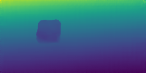
Fig. 3(a)-3(l) shows the results of the proposed experiments. The trained models are evaluated on several real-world depth images. In those images, the box is placed on a table. We present the results of scenes with increasing difficulty. In the first scene, the object is placed at the center of the scene, and no obstacles are present. In the second scene, two obstacles are placed next to the target object. The obstacles are also box-shaped but have different sizes than the target object. In the third scene, the target object is only partially visible, and there are two obstacles present. In Fig. 3(c),3(g),3(k), we present examples of reconstructed input depth images from Fig. 3(b),3(f),3(j) with different condition vectors.
In the presented cases, the cubes can be reconstructed at the desired poses.
The networks are able to extrapolate the background to complete the depth images at the original cubes’ locations.
We noticed that the reconstructions with the basic CAE model were considerably more blurry than the presented results of the CAE with Generator in Fig. 3(c),3(g),3(k).
This suggests that the additional component in the network architecture makes the trained model more expressive.
Both models are able to reconstruct the background plane from the input images well. The obstacles in 3(g) and 3(k) are also visible in the generated images, but they are less sharp than the target objects. During the development process of the method, we saw that the background reconstruction quality was higher when training with a simple reconstruction loss instead of using the weighted loss function on labeled pixels, described in Sec. III-B. However, for a good likelihood estimation the accurate reconstruction of the target object is of greater importance, so we compromised in the background reconstruction abilities.
Imperfections in the reconstruction of the background can lead to a constant bias on the loss for each queried state vector. Scaling the loss values to unit range can alleviate the bias.
As shown in Figs. 3(d),3(h),3(l), the likelihood functions of the learned models have their minima at the ground truth object states for the translational directions.
In all cases, these minima are global among the queried states.
The asymmetric shape of the loss functions correlates to the change of scale when the object is moved along the axes.
The same effect can be observed in the Synthetic&Synthetic benchmark.
In general, the shape of the loss along the axes follows the Synthetic&Synthetic benchmark well, suggesting that the model performs well on the posed problem.
Compared to the benchmark Input&Synthetic, it stands out that our method does not suffer from self occlusions while the benchmark does. Especially for translations along the object’s z-axis, the input image fully occludes the synthetic image in the benchmark case while the learned model can remove the box at its original pose.
The loss function exhibits symmetries when evaluating it along the rotational directions for the test object. Since the height (z-direction) differs from its depth (x-direction) and width (y-direction), the depth images should be identical for rotation of around x and y-axis and of around z-axis.
The expected symmetries can be observed with the CAE with Generator model for rotations in directions.
The basic CAE model cannot produce a reasonable likelihood function for rotations around the defined axes.
We hypothesize that the reconstruction of objects with the correct orientation is harder to achieve than with the correct translation since a smaller change in loss is observed when changing orientation compared to translation.
IV-B Particle Filter Integration
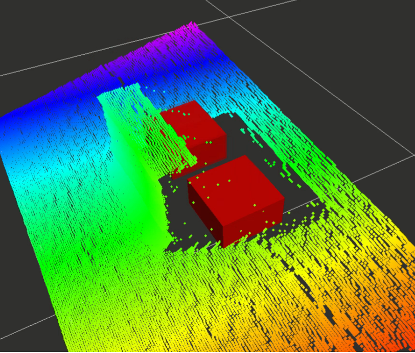
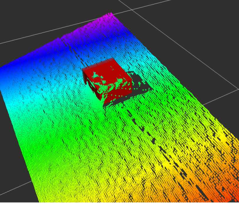
We integrate the DMU model with a particle filter implementation. DMU is used to compute weights for the re-sampling step during the measurement update. The normalizing factor is computed as the sum of all particle weights. A static depth camera observes a scene with two obstacles and a target object placed on a table. At the beginning of the experiment, the target object is hidden behind one of the obstacles. The two obstacles are then removed one by one such that the target object becomes visible.
Results
The accompanying video222https://youtu.be/MtTNIRcKBbk features the described experiment. Fig. 4 shows selected stills from one experiment. For better visibility, we chose a one-dimensional initial distribution with 100 particles, while for other experiments featured in the video, the particles are randomly placed on the table. After a few DMU steps, the particle distribution becomes bimodal with clusters of particles behind the two obstacles. Even though the target box is not visible yet, DMU can leverage the knowledge of observed free space to eliminate some particles. After removing the first obstacle and revealing that the target has not been hidden here, the particle distribution collapses, and only the particles behind the second obstacle remain. Finally, the target cube is visible in the depth image, and the filter converges to the ground truth box location.
IV-C Articulation State Estimation
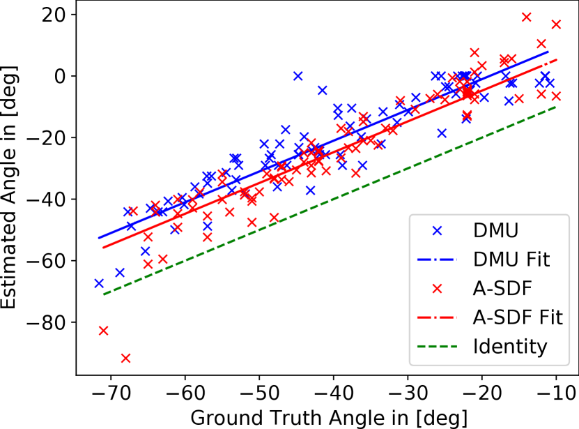
We compare DMU’s ability to infer the articulation state of an object to A-SDF as a baseline solution. The comparison is made on the laptop sequences of the RBO dataset. For each sequence, 10 depth images were selected by the authors of A-SDF for evaluation. We train the DMU network on synthetic depth images with a laptop placed on a table with varying positions, orientations, and opening angles. The system state is the opening angle, and the position and orientation are part of the unmodeled state. For each image of the test sequences, we compute the likelihood of possible joint angles. The angle with the highest likelihood is the estimate.
Results
Fig. 5(a) shows the estimated articulation states computed with both DMU and A-SDF for the sequences . Tab. 5(b) reports the mean average error (MAE) on the entire dataset and different subsets. While A-SDF is generally more accurate in articulation angle estimation, the inference time of our method is three orders of magnitude smaller, making it practical for real-time applications. We have observed an estimation bias for both methods with respect to the ground truth labels. Visual inspection of the depth images from the dataset and synthetic data generated by the simulator lets us conclude that the ground truth labels were biased. We report the bias compensated MAE as well and see similar accuracies for DMU and A-SDF.
| DMU | A-SDF | |
|---|---|---|
| MAE | - | |
| MAE A-SDF subset | ||
| MAE visualized subset | ||
| MAE unbiased | ||
| Inference time |
IV-D Articulation State and Object Pose Estimation
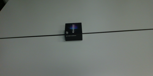
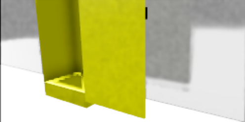
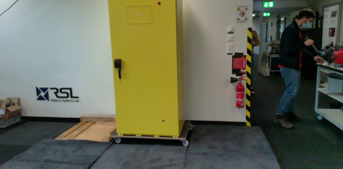
In this experiment, we evaluate the CAE model in a scenario where the network condition variables are the pose and the door opening angle of the switchboard cabinet shown in Fig 3(q). In particular, estimating the state of a door represents a common challenge in the current robotics manipulation research with increasing attention in recent years [30], [31]. For this experiment, the modeled state of the system is defined as , where are the planar position coordinates of the cabinet in a camera-fixed gravity-aligned coordinate frame, is the rotation of the cabinet around the vertical axis of that frame, and is the door opening angle. Following the notation introduced in Sec II-A, the unmodeled state of the system is represented by the walls and floor in the background image. For training, the CAE model without the additional generator network has been used. During evaluation on images from a real dataset, we observed a significant presence of outliers in the depth map. Those outliers are undetected points to which the sensor assigns depth. To increase robustness against outliers, the loss function was modified to mask out the extremes of the normalized depth interval, thus avoiding the undetected points to be decoded as close points.
Results
Results are presented in Fig. 3(m)-3(t). We evaluate the CAE on two depth input images, acquired from the synthetic data generator described in Sec. III-B and from a real dataset, respectively. The loss function is plotted as a function of the considered four-dimensional state. In the synthetic test-case, the CAE model gives comparable results as the Synthetic&Synthetic and the Input&Synthetic benchmarks. The loss function plots of Fig. 3(p) all have a minimum at the ground truth state, which shows that the network succeeds in learning the dependency on the state. This is in accordance with the generated image of Fig. 3(o), where a new depth image is reconstructed at a specified door angle.
Evaluation for the real test scenario (last row of Fig. 3) is more challenging due to the considerable measurement noise in the input depth image, shown in Fig. 3(r). The CAE model proves to be robust against the measurement noise and, as for the synthetic test, is able to generate different images at specified door angles. The performance of the learned model in estimating the likelihood is on par with the Synthetic&Synthetic benchmark, the upper bound of what can be achieved with the proposed method. It outperforms the Input&Synthetic benchmark, which fails for translations in direction and rotations around due to self occlusions.
V CONCLUSIONS & FUTURE WORK
DMU has shown to be a general framework to derive measurement update rules for Bayes filters. The learned models outperform the synthetic data baseline solution in the accuracy of the computed likelihood. Even though the models are only trained on synthetic data, they perform well on real-world data, too. Compared to A-SDF, we report a 1000x inference speedup in articulation state estimation, making the deployment in robotic applications feasible.
Furthermore, a particle filter using DMU offers interesting perspectives for active perception. In a scenario such as the example shown in Fig. 4(b) where the particle filter proposes two possible regions where a target object could be hidden, a robot can be commanded to explore those regions actively.
Solely providing depth information, the learned models have to rely on geometric properties to distinguish the modeled and unmodeled aspects of the observed system. We identified this as the major limitation during the inspection of failure cases on the RBO dataset. In future work, we would like to use RGB images as well, since texture greatly simplifies the detection of important features in complex scenes. Extending this work to RGB-D images poses additional challenges, because the unmodeled state dimension is much larger than for depth-only, increasing the imbalance between background and state dimensionality. Instead, we propose to use segmentation masks as an additional input since they are easy to obtain from the simulator for training and from a separate instance segmentation network for deployment.
References
- [1] J. Redmon, S. Divvala, R. Girshick, and A. Farhadi, “You only look once: Unified, real-time object detection,” in Proceedings of the IEEE conference on computer vision and pattern recognition, 2016, pp. 779–788.
- [2] K. He, G. Gkioxari, P. Dollár, and R. Girshick, “Mask r-cnn,” in Proceedings of the IEEE international conference on computer vision, 2017, pp. 2961–2969.
- [3] Y. Xiang, T. Schmidt, V. Narayanan, and D. Fox, “Posecnn: A convolutional neural network for 6d object pose estimation in cluttered scenes,” in Robotics: Science and Systems (RSS), 2018.
- [4] S. Thrun, W. Burgard, and D. Fox, Probabilistic robotics. Cambridge, Mass.: MIT Press, 2005.
- [5] M. Montemerlo, S. Thrun, D. Koller, and B. Wegbreit, “Fastslam: A factored solution to the simultaneous localization and mapping problem,” in Eighteenth National Conference on Artificial Intelligence. USA: American Association for Artificial Intelligence, 2002, p. 593–598.
- [6] R. Salakhutdinov and G. Hinton, “Deep boltzmann machines,” in Artificial Intelligence and Statistics, 2009, pp. 448–455.
- [7] G. E. Hinton, S. Osindero, and Y.-W. Teh, “A fast learning algorithm for deep belief nets,” Neural computation, vol. 18, no. 7, pp. 1527–1554, 2006.
- [8] I. Goodfellow, J. Pouget-Abadie, M. Mirza, B. Xu, D. Warde-Farley, S. Ozair, A. Courville, and Y. Bengio, “Generative adversarial nets,” in Advances in Neural Information Processing Systems, 2014, pp. 2672–2680.
- [9] D. P. Kingma and M. Welling, “Auto-encoding variational bayes,” in 2nd International Conference on Learning Representations, ICLR 2014, Banff, AB, Canada, April 14-16, 2014, Conference Track Proceedings, 2014.
- [10] K. Sohn, H. Lee, and X. Yan, “Learning structured output representation using deep conditional generative models,” in Advances in Neural Information Processing Systems, 2015, pp. 3483–3491.
- [11] D. J. Rezende, S. Mohamed, and D. Wierstra, “Stochastic backpropagation and approximate inference in deep generative models,” in International conference on machine learning. PMLR, 2014, pp. 1278–1286.
- [12] C. Winkler, D. Worrall, E. Hoogeboom, and M. Welling, “Learning likelihoods with conditional normalizing flows,” arXiv preprint arXiv:1912.00042, 2019.
- [13] S. Zakharov, I. Shugurov, and S. Ilic, “DPOD: 6D Pose Object Detector and Refiner,” in 2019 IEEE/CVF International Conference on Computer Vision (ICCV), Oct. 2019, pp. 1941–1950.
- [14] Y. Li, G. Wang, X. Ji, Y. Xiang, and D. Fox, “DeepIM: Deep Iterative Matching for 6D Pose Estimation,” International Journal of Computer Vision, vol. 128, no. 3, pp. 657–678, Mar. 2020.
- [15] J. Mu, W. Qiu, A. Kortylewski, A. Yuille, N. Vasconcelos, and X. Wang, “A-SDF: Learning disentangled signed distance functions for articulated shape representation,” in Proceedings of the IEEE/CVF International Conference on Computer Vision (ICCV), October 2021, pp. 13 001–13 011.
- [16] R. Martín-Martín, C. Eppner, and O. Brock, “The RBO dataset of articulated objects and interactions,” The International Journal of Robotics Research, vol. 38, no. 9, pp. 1013–1019, 2019.
- [17] R. G. Krishnan, U. Shalit, and D. Sontag, “Deep Kalman Filters,” arXiv:1511.05121 [cs, stat], Nov. 2015, arXiv: 1511.05121.
- [18] P. Becker, H. Pandya, G. Gebhardt, C. Zhao, C. J. Taylor, and G. Neumann, “Recurrent Kalman Networks: Factorized Inference in High-Dimensional Deep Feature Spaces,” in International Conference on Machine Learning. PMLR, May 2019, pp. 544–552.
- [19] M. Karl, M. Soelch, J. Bayer, and P. van der Smagt, “Deep variational bayes filters: Unsupervised learning of state space models from raw data,” in 5th International Conference on Learning Representations, ICLR 2017, Toulon, France, April 24-26, 2017, Conference Track Proceedings, 2017.
- [20] P. Karkus, D. Hsu, and W. S. Lee, “Particle filter networks with application to visual localization,” in Proceedings of The 2nd Conference on Robot Learning, ser. Proceedings of Machine Learning Research, A. Billard, A. Dragan, J. Peters, and J. Morimoto, Eds., vol. 87. PMLR, 29–31 Oct 2018, pp. 169–178.
- [21] T. Avant and K. A. Morgansen, “Rigid Body Dynamics Estimation by Unscented Filtering Pose Estimation Neural Networks,” in 2020 American Control Conference (ACC), Jul. 2020, pp. 2580–2586.
- [22] R. Liu, J. Lehman, P. Molino, F. Petroski Such, E. Frank, A. Sergeev, and J. Yosinski, “An intriguing failing of convolutional neural networks and the coordconv solution,” in Advances in Neural Information Processing Systems, 2018.
- [23] M. Danielczuk, M. Matl, S. Gupta, A. Li, A. Lee, J. Mahler, and K. Goldberg, “Segmenting unknown 3d objects from real depth images using mask r-cnn trained on synthetic data,” in 2019 International Conference on Robotics and Automation (ICRA). IEEE, 2019, pp. 7283–7290.
- [24] T. M. Iversen, A. G. Buch, and D. Kraft, “Prediction of ICP pose uncertainties using Monte Carlo simulation with synthetic depth images,” in 2017 IEEE/RSJ International Conference on Intelligent Robots and Systems (IROS), 2017, pp. 4640–4647.
- [25] C. Wan, T. Probst, L. Van Gool, and A. Yao, “Crossing nets: Combining gans and vaes with a shared latent space for hand pose estimation,” in Proceedings of the IEEE Conference on Computer Vision and Pattern Recognition, 2017, pp. 680–689.
- [26] D. P. Kingma and J. Ba, “Adam: A method for stochastic optimization,” in 3rd International Conference on Learning Representations, ICLR 2015, San Diego, CA, USA, May 7-9, 2015, Conference Track Proceedings, Y. Bengio and Y. LeCun, Eds., 2015.
- [27] G. Pitteri, M. Ramamonjisoa, S. Ilic, and V. Lepetit, “On object symmetries and 6d pose estimation from images,” in 2019 International Conference on 3D Vision (3DV). IEEE, 2019, pp. 614–622.
- [28] E. Corona, K. Kundu, and S. Fidler, “Pose estimation for objects with rotational symmetry,” in 2018 IEEE/RSJ International Conference on Intelligent Robots and Systems (IROS). IEEE, 2018, pp. 7215–7222.
- [29] J. Richter-Klug and U. Frese, “Handling object symmetries in cnn-based pose estimation,” arXiv preprint arXiv:2011.13209, 2020.
- [30] M. Arduengo, C. Torras, and L. Sentis, “Robust and adaptive door operation with a mobile robot,” Intelligent Service Robotics, pp. 1–17, 2021.
- [31] M. Mittal, D. Hoeller, F. Farshidian, M. Hutter, and A. Garg, “Articulated object interaction in unknown scenes with whole-body mobile manipulation,” arXiv preprint arXiv:2103.10534, 2021.